An Experimental Water Consumption Regression Model for Typical Administrative Buildings in the Czech Republic

Abstract

Pressure management is the basic step of reducing water losses from water supply systems (WSSs). The reduction of direct water losses is reliably achieved by reducing pressure in the WSSs. There is also a slight decrease in water consumption in connected properties. Nevertheless, consumption is also affected by other factors, the quantification of which is not trivial. However, there is still a lack of much relevant information to enter into this analysis and subsequent decision making. This article focuses on water consumption and its prediction, using regression models designed for an experiment regarding an administrative building in the Czech Republic (CZ). The variables considered are pressure and climatological factors (temperature and humidity). The effects of these variables on the consumption are separately evaluated, subsequently multidimensional models are discussed with the common inclusion of selected combinations of predictors. Separate evaluation results in a value of the N₃ coefficient, according to the FAVAD concept used for prediction of changes in water consumption related to pressure. The statistical inference is based on the maximum likelihood method. The proposed regression models are tested to evaluate their suitability, particularly, the models are compared using a cross-validation procedure. The significance tests for parameters and model reduction are based on asymptotic properties of the likelihood ratio statistics. Pressure is confirmed in each regression model as a significant variable.

1. Introduction

The volume of water consumed per unit of time is the operating parameter of each water supply system. Great attention is currently paid to optimizing the pressure conditions in water supply systems. However, a major part of the optimizing approaches is dedicated to reduction of both water loss and energy cost [1,2]. The first step in reducing water losses is usually the revision of pressure conditions and their subsequent adjustment, enabling the optimum scope of pressure conditions while maintaining the hydraulic capacity of the mains. In most cases, pressures in the network are decreased to achieve reduced water loss and lower failure rates of the mains. Yet, evidently, with lowered pressure there is also a decrease in the volume of water billed to the individual consumers. Therefore, lowering the pressure in the network has a positive effect on water loss while having a negative effect on the volume of billed water and the economic performance of the company. In our experience in regard to this solution of optimization, waterworks operators stress the following criteria, listed in a decreasing order according to priority: (1) the economic aspect—the problem of water loss is solved strictly from an economic viewpoint. The effectiveness of each proposed measure is always calculated from the economic perspective of the company. Measures with negative economic effects are only implemented under the condition that they generate a significant secondary benefit other than economic (for example, environmental); (2) the environmental viewpoint—in cases where it is a relevant problem within the given situation, the capacity of the water source is considered. Reduction of water loss presents a decreased burdening of the source and the ecosystem as a whole; (3) quality of delivered water—reduction of water loss causes a decreased consumption of water, increasing the age of water in the network and, in specific cases, this may result in a higher frequency of complaints regarding its quality. This point of view is always considered individually with regard to the specific situation; (4) company prestige—last in terms of priorities, yet still a relevant criterion. Performance indicators of water companies are annually published in a country-wide professional almanac. Achieving outstanding results in the category of water loss is a matter of prestige.

In order for such water consumption to be included as a criterion in the optimization of pressure conditions, it is necessary to express it mathematically as a function of pressure. This mathematical description complicates its stochastic nature, as is apparent, for example, from [3]. It has been proven that many more factors aside from pressure conditions have an effect on water consumption. Several previous studies have shown that water consumption is affected not only by customer price [4,5,6], but also by climate factors [6,7,8] and pressure in the water mains [2,5,9,10]. For example, in [11] an analysis of the dependency of water produced for the city of Brno on meteorological factors was conducted and a certain dependency was indicated. This analysis was carried out for the entire water supply system. On the other hand, it should be noted that for each type of user the dependency on factors influencing consumption always varies (see e.g., [12]). According to [13] water consumption is divided for the purposes of simulating the changes in water consumption with pressure changes into “inside-the-house” and “outside-the-house”. Both areas of consumption then have different coefficients expressing their dependency on pressure. Subsequently, the average coefficient expressing dependency of pressure for the entire building and for each consumer is calculated. Subsequently, this cumulative coefficient per user is implemented into the FAVAD (Fixed and Variable Discharge) equation according to [14], or into its simplified form according to [13].

Nowadays, there are not many N₃ set coefficients within the meaning of [13] based on real studies. For example the value of the “inside-the-house” consumption coefficient was set at 0.2 for the Johannesburg student campus at the University of Johannesburg in [15]. Also worth mentioning is the principle of minimum pressure, which must be ensured in the water supply network so that the water supply can be realized. If this value is under-stepped, the volume of water supplied is considered zero [9]. In this study, the results of which are presented here, this limit was defined by valid legislation at 0.15 MPa and was not broken during the experiment.

This paper provides information regarding the effect of water pressure and selected climatological factors on water consumption in an administrative building. It had three goals.

The first was to establish the value of the N₃ coefficient used in the FAVAD concept. In the past, a sufficient number of studies used the FAVAD concept, covering the entire spectrum of various types of end users. A new regressive model was not created for this purpose, but an existing model used according to [13].

The second goal was to verify whether it is possible to predict water consumption under stable pressure conditions (albeit with various levels of pressure) on the basis of climatological factors, using linear regression.

The third goal was to extend the FAVAD concept into the area of water consumption prediction, according to [13] and stipulate a regressive model with a newly added variable of climatological factor. All regression models were subject to statistical testing to confirm or reject their significance.

2. Materials and Methods

2.1. Facility Details, Measuring Campaign and Measuring Equipment

2.1.1. Facility Details

The case study was conducted on an office-type building, which is a very common kind of office facility in the CZ. The building under study has three above-ground floors and the maximum number of workers is 35. The detailed layout of the building with distribution of workers within the floors is well apparent from Figure A1. The workers are evenly allocated on all floors, each of them equipped with similar fittings. The toilets are fitted exclusively with volumetric flushing systems with a pre-stored storage water tank. There are no pressure flushers in the building. There are also no showers.

The survey determined that, in the meaning of [13], all measured water was consumed “inside the house”. Characteristic flow rates for this building are shown in

Table A1. Characteristic values of water consumption during working hours.

Day (Working Hours)	Minimal Consumption (Liters)	Mean Consumption (Liters)	Maximal Consumption (Liters)
Monday + Wednesday (7–17)	608	892	1307
Tuesday + Thursday (7–15)	481	710	1252
Friday (7–13)	307	623	927
All days (7–13)	307	545	982
Hourly consumption—all days	10	91	381

. Working hours of one five day working week had three different periods. The period of working hours in the individual days for Mondays and Wednesdays is from 7:00–17:00, on Tuesdays and Thursdays 7:00–15:00 and on Friday 7:00–13:30. The working day lengths for individual days remained the same over the course of the entire duration of the measuring campaign.

2.1.2. Measuring Campaign

The main part of the measuring campaign study was divided into several shorter periods of time corresponding to the measurement cycles. Within one measuring cycle, the pressure reducing valve (PRV) setting was set constant. The length of the measurement cycle was approximately 14 days (i.e., 10 working and 4 weekend days), with possible fluctuations due to specific circumstances such as public holidays etc. The length of the cycle was determined with respect to allowing very low or very high temperatures or humidity to occur in multiple cycles, as these extremes occurred in the shorter term.

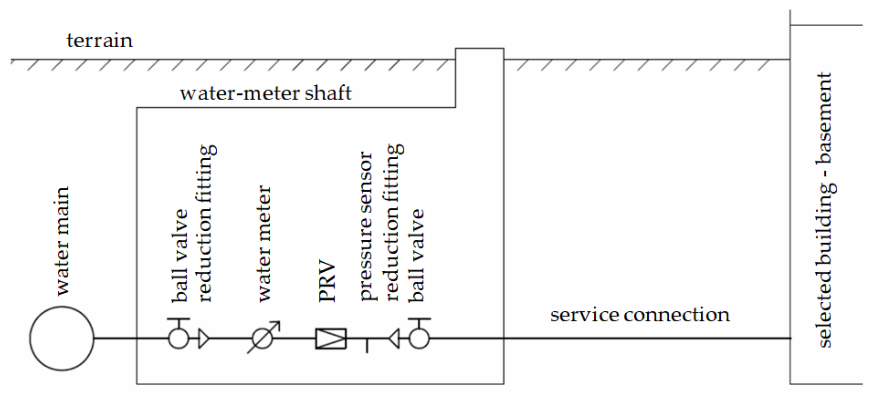
Because it was not possible to change the pressure conditions in the entire pressure zone of the water network, the measuring devices were attached to the water hook-up in the immediate vicinity of the water mains. These devices included (in the direction of the water flow) flow-rate measurement, pressure reducing valve “PRV”, and pressure sensor (see Section 2.1.3). The diagram of the connection of these measuring devices is apparent from Figure A2. The installation in the immediate vicinity of the water mains ensured analogous conditions to a change of pressure conditions in the entire network.

The output pressure of PRV was determined individually for each measuring cycle. The value of the output pressure was changed in leaps. The limiting conditions to the minimum output pressure of the PRV valve were taken into account, in order to remain consistent with the legislation of the CZ, e.g., to ensure minimal pressure or normal operation in the building. According to [16], the minimal pressure in the hook-up in the CZ is 0.15 MPa, however due to the complaints by workers it was not possible to reduce the pressure to this value. There was an attempt to set the output pressure in a manner that the average pressure during working hours was in the middle interval in the given category. However, this was not always achieved, particularly due to unplanned interventions with the measuring devices.

2.1.3. Measuring Device

The following devices were used for measuring:

• Change of pressure conditions—a spring-based PRV with the output pressure range of 0.15–0.60 MPa was used. The hydraulic losses caused by the PRV were low even at the maximum hourly flow rate. PRV dimension was chosen with respect to the hydraulic losses and characteristic flow rates through the PRV. The characteristic flow rates in the given building are presented in Table A1 and the PRV head loss diagram is shown in Figure A3.
• Flow volume measurement—The volume of water flowing was measured using a water meter with a pulse generator and the pulse value of 1 liter. The water meter corresponded to the “C” level of precision in the sense of [17]. Nominal flow rate of the water meter in the sense of [17] is 2.5 m³ h⁻¹. In order to sustain the guaranteed precision, undisturbed spacing lengths were maintained both upstream and downstream of the water meter. The value of the pressure was recorded along with the water meter value every 15 s. This was an interrupted measurement with a relatively short time period.
• Pressure measurement—The pressure was measured with an integrated pressure sensor with a range of 0.0–1.0 MPa, and measurement accuracy of 0.25% of the range (i.e., 0.0025 MPa).

2.2. Data and Its Verification

The data set consists of daily observations of the total volume of water consumed and the pressure on connection in the period from September 2016 to September 2017. Aside from the variables of interest to be further embedded into a model (see Section 2.3), the observations were also accompanied by other metadata. Those included the actual number of employees at the workplace, their working time (varying daily between 6.5 and 10 h, see Section 2.1.1), and indication of extraordinary events that could significantly affect water consumption. The climatological covariates, i.e., temperature and humidity, were obtained from the Czech Hydrometeorological Institute in the form of a series with resolutions of one hour. The relative daily values of the meteorological covariates were observed by averaging measurements corresponding to the working time during the current day.

First, in order to compare the water consumption under specific day conditions, the normalized consumption was determined with respect to the actual number of employees and the working-time duration. The total consumption may be affected by fluctuation of employees during each particular shift. However, an initial survey found that employees spent the vast majority of their working time in the office. On account of that, a simplifying assumption of constant number of workers was made. Thus, for a given $i$-th day the normalized water consumption $C_i$ ($\mathrm{l}·{\mathrm{person}}^{-1}·{\mathrm{hour}}^{-1}$) was evaluated as follows

$$C_i=\frac{V_i}{p_i{h}_i},$$

(1)

where $V_i$ denotes the total water consumption, $p_i$ is the number of employees, and $h_i$ is the number of working hours during the $i$-th day, respectively. This standardized quantity is considered to be independent of current circumstances in the office. Since any further analysis is based purely on this variable, from here on we refer to normalized consumption simply as consumption.

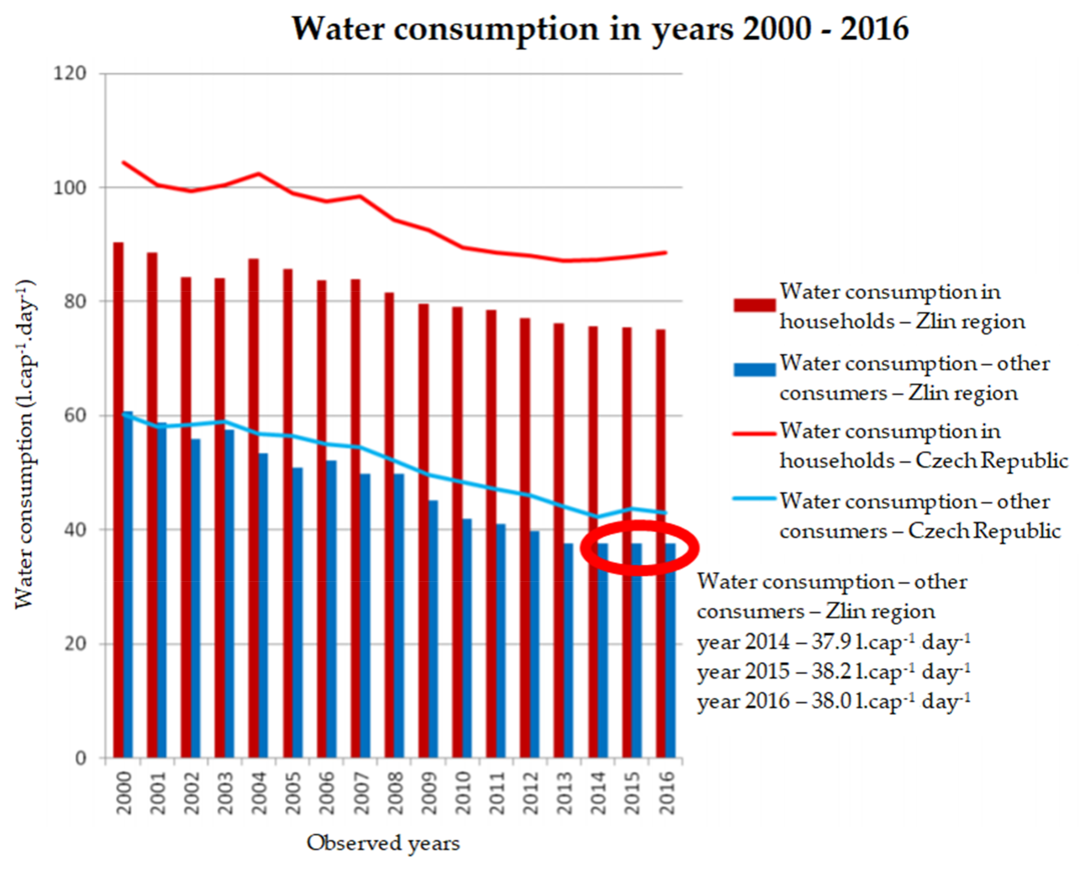
As the observation period lasted one year, usually certain long-term impacts had to be taken into account, i.e., an inter-annual trend or cyclic components commonly related to a period of the year. In the CZ there has been a downward trend in both total water consumption and water consumption per capita since 1989. Nevertheless, as discussed e.g., in [18,19], in the last three years the total consumption for the CZ is considered rather stable from a global perspective, particularly in the Zlin region (in which this case study was performed).

As is apparent from Figure A4, consumption for the last three years is practically stable for the “other users” group to which this case study belongs. The overall annual consumption in the given administrative building in the last three years only differs in the range of tens of a percent (239.6 m³–238.3 m³–241.1 m³), while the maximum number of workers per shift continued to be the same.

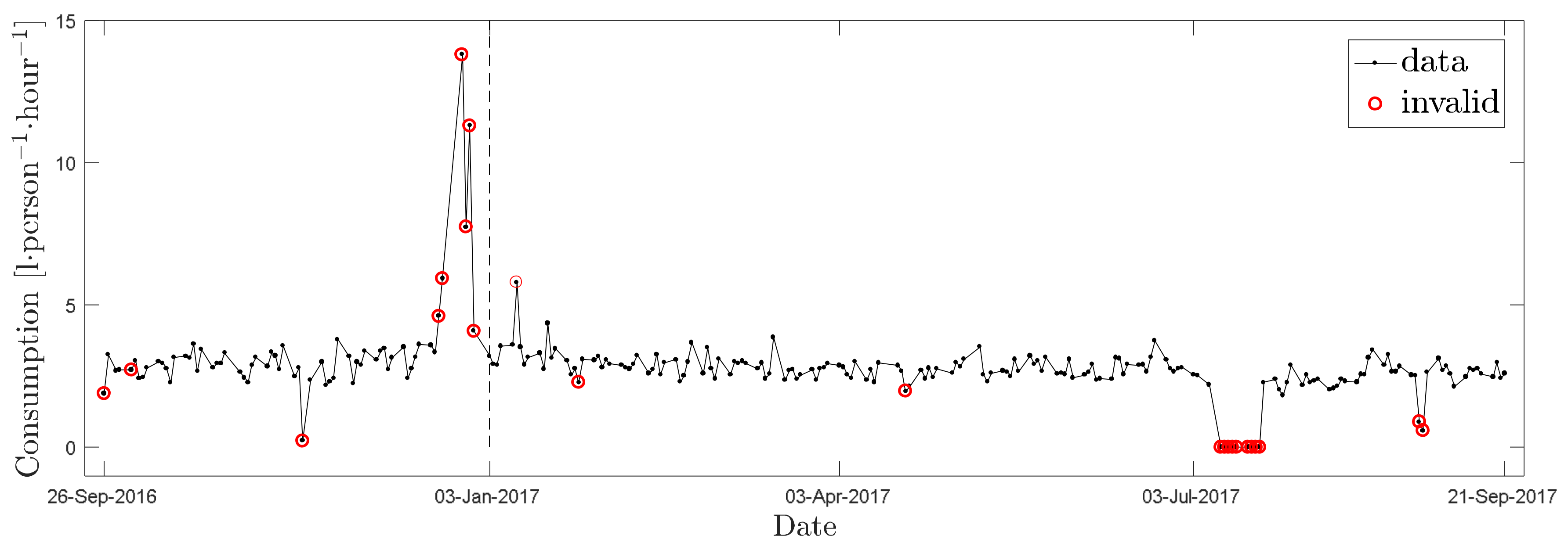
In Figure 1 the time dependency of the consumption is visualized in the period of interest. As is evident from Figure 1, as well as from the plot of first differences (not shown) there is no significant trend to be embedded into a model. Hereby we follow the results obtained in [18,19] and put no specific emphasis on any trend component. Moreover, especially due to focus of the study on an office building, the data exhibits no seasonal effects. This agrees with the authors’ experiences within similar facilities in the area of CZ. All consumption during the working hours is “inside-the-house” in the sense of [13] and no irrigation or gardening is performed. In general, the latter two usually represent the main part of the seasonal increments in consumption. Hence, the mean water consumption is considered to remain stable over the year.

In order to exclude unreliable measurements observed under extraordinary conditions, the metadata was closely investigated. The outliers could seriously harm any further analysis and lead to significant bias in estimates of the dependency structure. There were several types of uncommon events identified. Particularly, from the data set all days labelled as anomalous were excluded. This includes mostly situations where significant volumes of water were used for other purposes than the routine needs of the office (see e.g., the peak at the end of year 2016 in Figure 1). Further, we removed those days in which the number of workers dropped below 10% of the office capacity, i.e., typically the holiday season. Moreover, data have been excluded from the days with uncommon behavior of the consumption aggregation monitored during the day. This typically indicates a failure of the measuring equipment. Altogether about 9% of available data was discarded, whereby we assumed the accuracy of any statistical inference should not be violated. A closer description of the excluded data is shown in

Table A2. Days excluded from the statistical analysis of data sets.

No.	Date	Day of Week	Problem Description	Explanation of Problem
1	26.09.2016	Monday	Zero consumption during 8–11	Technical problems with measuring device
2	03.10.2016	Monday	Unknown consumption during 9–11
3	16.11.2016	Wednesday	Very low consumption per person	Failure of water supply—water mains breakage—failures duration 6 h
4	21.12.2016	Wednesday	Very high consumption per person	Very low number of workers—Christmas holidays + 7 visitors over the course of approximately 4 h
5	22.12.2016	Thursday		Very low number of workers—Christmas holidays + 15 visitors over the course of approximately 2 h
6	27.12.2016	Tuesday		Very low number of workers—only accountants present + creation of an ice rink
7	28.12.2016	Wednesday
8	29.12.2016	Thursday		Very low number of workers—only accountants present + some workers outside the evidence
9	30.12.2016	Friday
10	10.01.2017	Tuesday		Excluded on the basis of Grubbs’ test results
11	26.01.2017	Thursday	Low consumption per person	8 left the building for an unknown number of hours
12	20.04.2017	Thursday		21 workers left the building for 5 h
13	10.07.2017	Monday	Negligible consumption per person	Very low number of workers—summer holidays—only workers in the reception—smaller number of workers in the complex than in evidence
14	11.07.2017	Tuesday
15	12.07.2017	Wednesday
16	13.07.2017	Thursday
17	14.07.2017	Friday
18	17.07.2017	Monday
19	18.07.2017	Tuesday
20	19.07.2017	Wednesday
21	20.07.2017	Thursday
22	30.08.2017	Wednesday	Very low consumption per person	19 workers left the building for 3.5 h
23	31.08.2017	Thursday		23 workers left the building for 4.5 h

.

By a stability assessment of the designed regression models (discussed below in Section 2.3), we identified significantly outlying observation at 10 January 2017 (the first invalid observation of the year 2017 in Figure 1). Although no extraordinary event was indicated in the metadata, this observation was additionally excluded. This decision is based both on visual inspection of the neighboring measurements in the consumption series, as well as on statistical criterion. For both models presented in Section 2.3, the corresponding standardized residual is more than three standard deviations from the residual mean. Moreover, the significance of the outlier was also indicated by Grubbs’ test [20] at significance level 0.05. Details are more closely discussed in Section 3.

2.3. Statistical Inference for Pressure

The main object of study is the assessment of dependence relations between consumption and monitored covariates, i.e., primarily the water pressure and climatological factors. The analysis was performed in two stages. First, the influence of the pressure was studied separately. From the practical point of view, unlike the meteorological inputs, the water pressure is the only operational variable that can be managed. Second, we considered all the factors and built a model for evaluation of their contribution to water consumption.

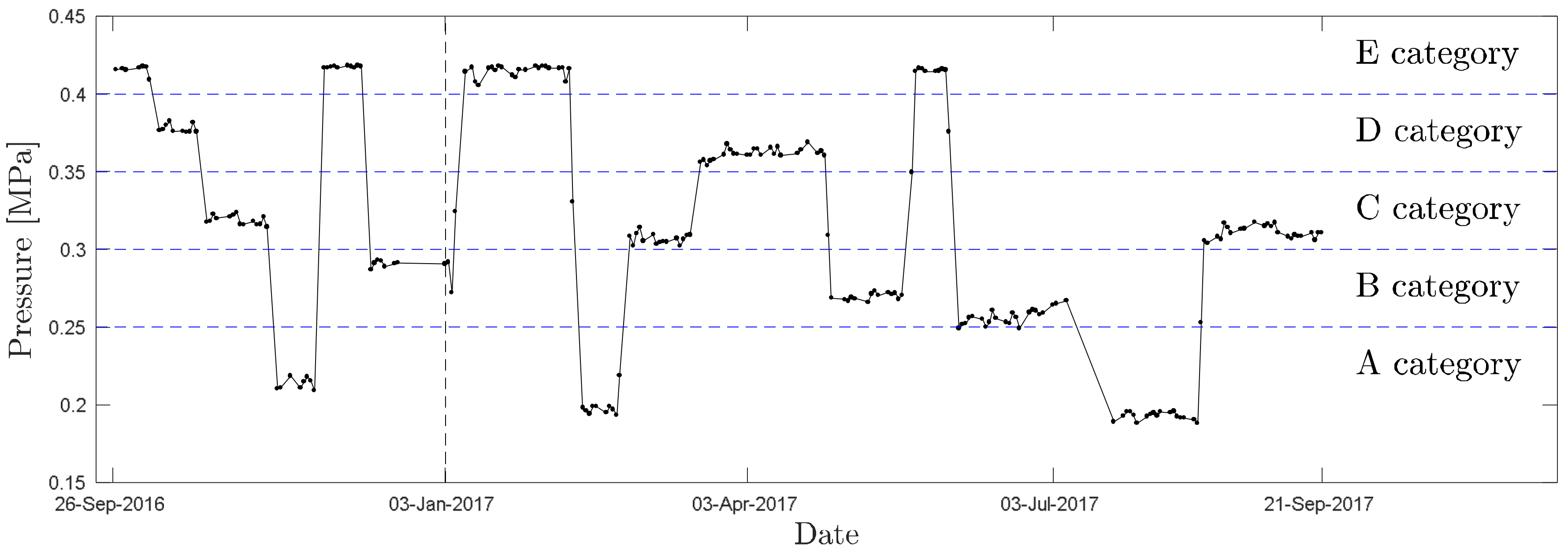
With respect to the experiment setup, the pressure observations were categorized as follows: category A (less than 0.25 MPa); category B (0.25 to 0.30 MPa); category C (0.30 to 0.35 MPa); category D (0.35 to 0.40 MPa) and category E (over 0.40 MPa). The changes in measurement cycles over time are shown in Figure 2.

Despite some variation of the pressure within a measurement cycle, the above mentioned categorization should preserve the classification of the PRV settings. Due to measurement accuracy discussed in Section 2.1.3, the observations are unlikely to overleap between diverse classes.

The statistical inference is based both on a linear model and its derivations, as well as nonlinear analysis. Initially, one-way analysis of variance (ANOVA) was performed to assess the significance of the dependency between the observed consumption and the water pressure categories. The necessary preconditions to ANOVA were verified using the Bartlett and Levene test for variance equality, the normality of the data was checked by goodness-of-fit test [21] (Pearson’s ${\chi }^2$, Lilliefors, and Anderson-Darling (A-D) test was applied, respectively).

To evaluate the effect of changes in pressure, a regression curve was fitted to the data by the means of the Least Squares (LS) method. For this purpose we consider in the first case a simple linear model of the form

$$C_i={\beta }_0+{\beta }_1{P}_i.$$

(2)

where $C_i$ denotes consumption in the meaning of (1) obtained under the pressure $P_i$ ($i=1,\cdots ,n$; $n$ is the number of observations). The model (2) is particularly meant as a possible local approximation of the relation between consumption and pressure. It is used primarily for performance comparison with a non-linear model discussed below. The regression parameter estimates are obtained as a common solution to the system of normal equations [22].

Usually, a non-linear dependence between consumption and pressure is considered. Hereby we follow the study [11] in which the authors introduced a relationship in the following form:

$$C_i=C_0{\left(\frac{P_i}{P_0}\right)}^{N_3},$$

(3)

where $C_0$ and $P_0$ denote the consumption and the pressure corresponding to the highest pressure category E, respectively. A curve similar to (3) was also applied in [11]. An advantage of the relation (3) stands in the simple interpretation of the coefficient N₃ as a measure of the pressure change to the water consumption. In our case, the coefficients N₃ and C₀ were considered as unknown regression parameters to be estimated. The pressure P₀ is assumed fixed, equal to the average of category-E pressures. The estimates of the regression parameters are obtained by the Maximum Likelihood (ML) method. Hence we obtained the values

$$C_i=C_0·p_i{}^{N_3}+{\epsilon }_i,$$

(4)

where $p_i=P_i/P_0$ is the normalized pressure, and ${\epsilon }_i$ are independent and normally identically distributed random variables following the distribution $\mathrm{N}\left(0,{\sigma }^2\right)$, where ${\sigma }^2>0$ is unknown. Given the observation $p_i$, the conditional density of $C_i$ is again normal with the expected value $C_0·p_i{}^{N_3}$ and variance ${\sigma }^2$. Thus, it can be derived that the logarithmic likelihood function $l\left(C_0,N_3,{\sigma }^2\right)$ takes the form

$$l\left(C_0,N_3,{\sigma }^2\right)=-\frac{n}{2}\log \left(2\mathsf{\pi }\right)-\frac{n}{2}\log {\sigma }^2-\frac{1}{2{\sigma }^2}{\displaystyle \sum }_{i=1}^n{\left(C_i-C_0{p}_i{}^{N_3}\right)}^2.$$

(5)

The ML estimates $\widehat{C_0}$, $\widehat{N_3}$, $\widehat{{\sigma }^2}$ of the parameters $C_0$, $N_3$, and ${\sigma }^2$ are obtained in order to maximize the relation (5). Note that ML estimates for the model (2) are the ordinary LS estimates. The use of the ML method, in general, gains a particular advantage in native estimation under the assumption of the non-linear model (4). The estimates follow good asymptotic properties and are suitable for further extensions of the model addressed later.

The significance test and confidence interval estimation for the parameters are based on likelihood ratio (LR) statistics

$$LR=2\left[l(\widehat{C_0},\widehat{N_3},\widehat{{\sigma }^2})-l(C_0{}^{\ast },N_3{}^{\ast },{{\sigma }^2}^{\ast })\right],$$

(6)

where the starred variables denote fixed values of the corresponding parameters to be tested against. Testing of a particularly selected parameter is accomplished with the LR test with nuisance parameters [22]. The LR statistics follows, under some regularity conditions, asymptotically ${\chi }^2$ distribution with degrees of freedom equal to the number of target parameters (or to the number of parameters if no nuisance parameters are present) [22]. Confidence boundaries for the parameter estimates are determined from the profile likelihood function [23,24,25]. In a rough description, for a given significance level $\alpha$, the values of the particular parameter are determined for which the LR test does not indicates significant deviations. Hence, the intersections between the logarithmic likelihood function need to be identified (in which the remaining parameters are held fixed and treated as nuisance parameters), and the threshold $\left[l(\widehat{C_0},\widehat{N_3},\widehat{{\sigma }^2})-{\chi }_1^2\left(1-\alpha \right)\right]$, where ${\chi }_1^2\left(1-\alpha \right)$ denotes the $\left(1-\alpha \right)$ quantile of the ${\chi }^2$ distribution with one degree of freedom.

In order to assess the performance and verification of both models (2) and (3), a $k$-fold cross validation was applied [26,27,28]. In order to assess the regression performance and verification a k-fold, cross validation was applied. Hence, the whole data set was partitioned into k sub-samples comparable in size. In k runs, the regression curve was evaluated using one of the k sub-samples as a testing set, while the remaining sub-samples served as a training set to fit the regression. Namely $k=10$ was chosen with respect to available data size. This choice has commonly been made for similar purposes. Given a regression curve estimated from the training set, as the performance criterion is taken the mean square error (MSE) of the testing subsample.

2.4. Statistical Inference for Climatological Factors

In the following, the contributions of selected climatological factors to the change in consumption are investigated. For the study, a series of daily averages of temperature and humidity are available. A procedure of variable addition into a model was discussed in [28]. Hereby the authors apply the forward selection of predictors with respect to correlation-based relations to the explained variable. In our case, however, it could be expected that the two climatological variables are physically linked to each other. If it were so, it would be inappropriate to include both predictors simultaneously since such a mis-specified model may be harmed by a large bias in parameter estimates.

Due to verification of such an assumption, attention was paid to the characteristics of possible correlation between them and the pressure. The pairwise Spearman’s rank correlation coefficients were evaluated and this was followed by their significance test. As discussed further in Section 3.3, both climatological covariates are inconsiderably related. The problem of inclusion of redundant covariates has been well discussed, for example, in the study [29]. Here the authors consider an evaluation framework for determination if a variable should be embedded to a model with respect to its explanation capability. This is especially suitable if large sets of variables are taken into account. In the case of our study, particularly because of evident relation between both climatological covariates, the inference is limited only to the instances, where the contribution of both factors is evaluated separately.

This was done in two ways. First we evaluated the influence of a selected covariate on consumption separately corresponding to particular categories of pressure. Here we assume a simple linear regression model of the form equal to (2) with the pressure $P_i$ replaced with other predictors of interest, i.e., either the temperature or the humidity. Inferences concerning the fit and estimated regression parameters are based on the usual properties of the linear model.

Subsequently we considered two extensions of the model (3) with embedded climatological covariates. Formally, we assume the relation

$$C_i=C_0{\left(\frac{P_i}{P_0}\right)}^{N_3}+\beta T_i,$$

(7)

where $C_0$, $N_3$, and $\beta$ are regression parameters to be estimated. The variable $T_i$ corresponds either to temperature or humidity, respectively, observed simultaneously with the consumption $C_i$.

The estimates of the parameters above are obtained again by the ML method. Following the assumptions of the model (4), the corresponding logarithmic likelihood function can be obtained in a form very similar to (5); the summands ${\left(C_i-C_0{p}_i{}^{N_3}\right)}^2$ in the last term are merely replaced by ${\left(C_i-C_0{p}_i{}^{N_3}-\beta T_i\right)}^2$. The use of the ML method is particularly suitable for hypotheses testing. We should be particularly interested in the determination of sub-model significance, i.e., whether the model (7) can eventually be reduced to (3). This is provided by the LR test where all the parameters from the model (4) are considered as nuisance parameters and the newly included parameter $\beta$ is tested for significance against a zero value.

3. Results

3.1. Outlier Identification

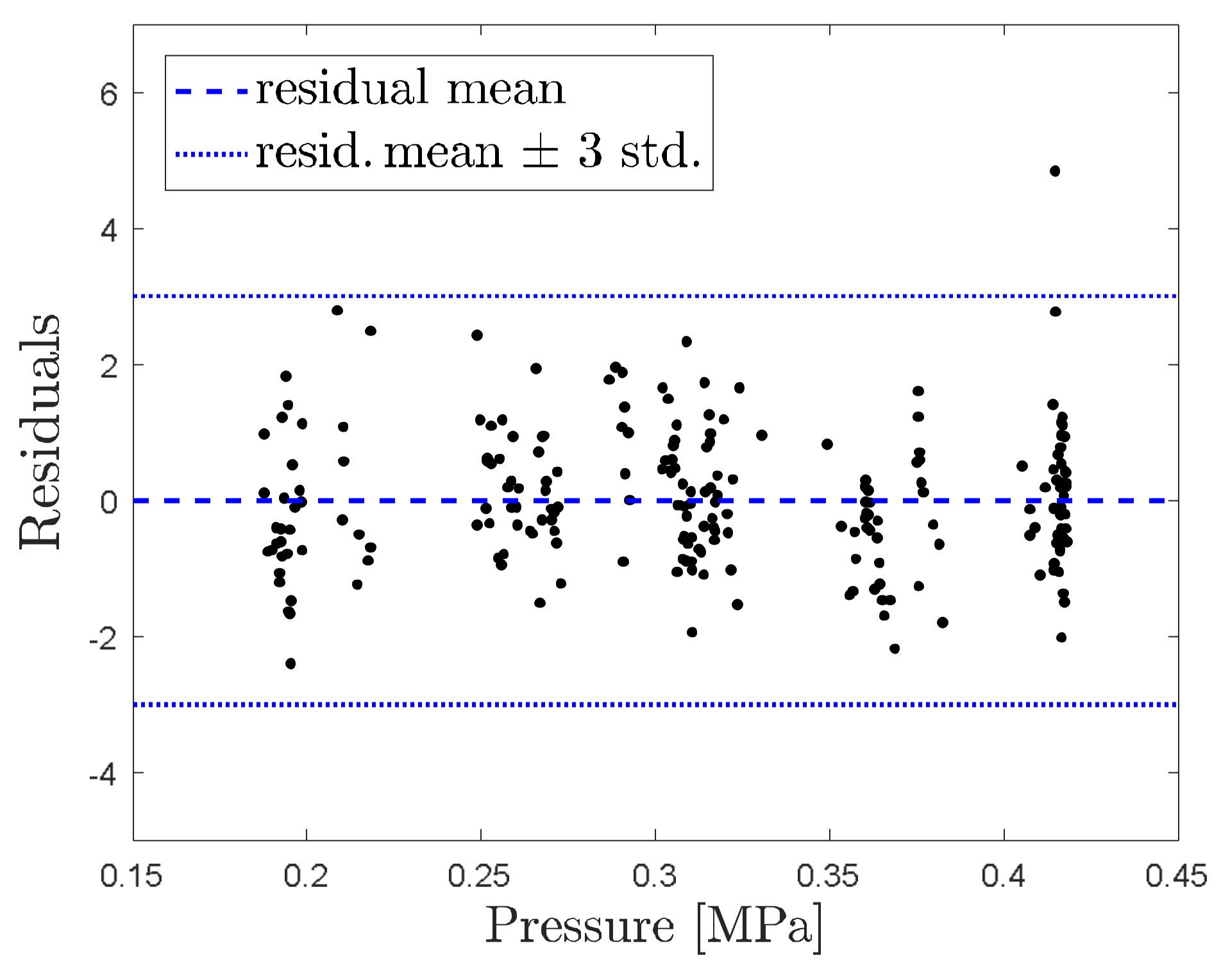
On account of available metadata, obviously invalid measurements were initially removed from the data indicating records of extraordinary events. A first approach to the reduced observations was made by a direct fit of the regression curve (3) to consumption measurements. Here we omit the suitability discussion of the curve and this will be discussed later in Section 3.2. In Figure 3 the standardized residuals of the fit are visualized along with their mean and confidence bounds of half-width equal to three standard deviations estimated from the residuals.

Isolated observations beyond these bounds on the right indicate the presence of an outlier. The behavior of the series in Figure 1 (at corresponding date 10 January 2017) agrees with this conclusion. The neighboring values report no significant difference from the remaining flow of the process. In order to achieve other than only visual arguments, the one-sided Grubbs’ test for outliers was applied. As expected, at a significance level of 0.05 the observation was determined as a significant outlier, with the Grubbs’ statistics equal to 4.81 (i.e., the value is almost five standard deviations distant from the residual mean).

The presence of an outlier in the series could seriously corrupt any further statistical inference leading to bias. Because of the presented results the corresponding observation was additionally removed from the data set and thus will not be taken into account in any further considerations.

3.2. Dependency of Consumption on Pressure

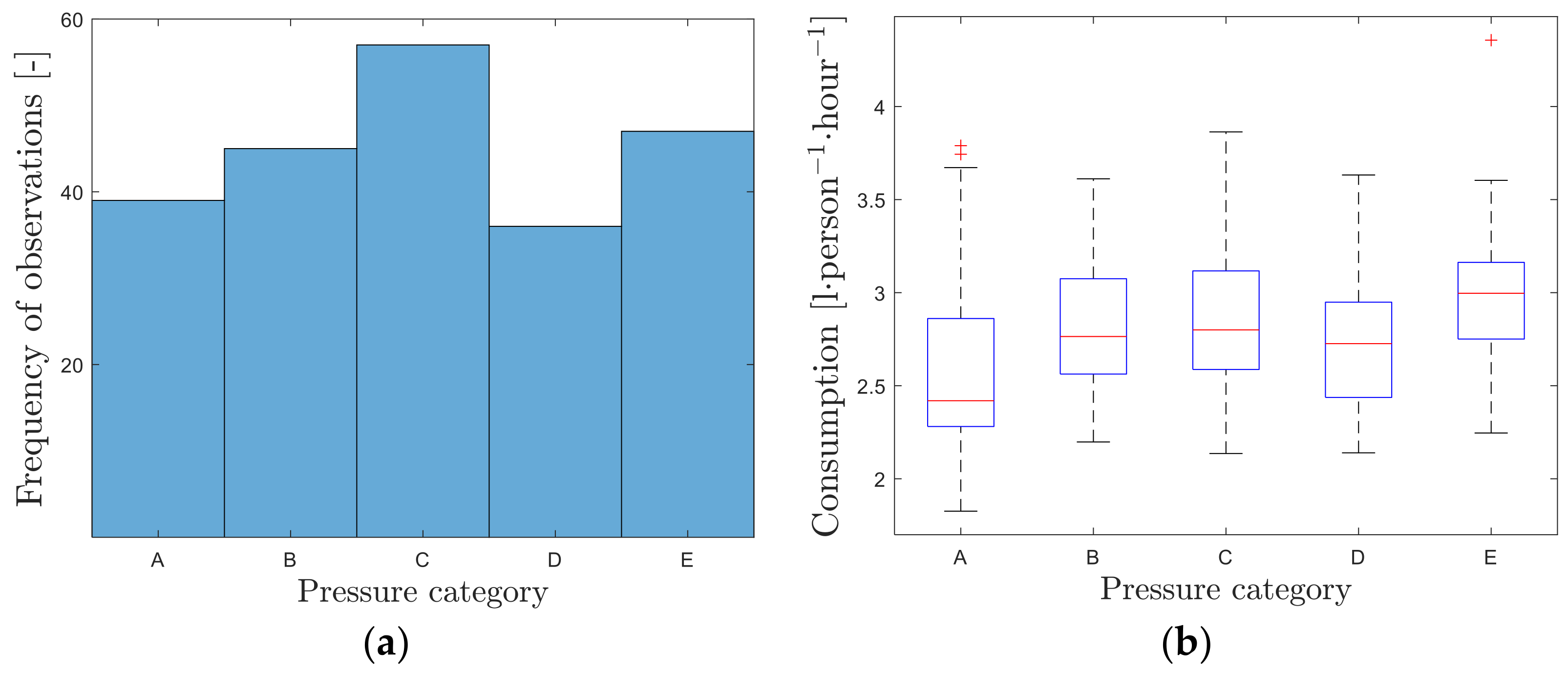
The remaining $n=224$ observations of pressure were categorized relative to the description in Section 2.2. Figure 4 illustrates the frequencies of the particular categories. As a consequence of measurement design, the categories are rather uniformly represented in terms of the frequencies. The boxplots of consumption are also visualized corresponding to specific pressure categories. The whiskers show, as is common, the 1.5 inter-quantile range.

In the first step a one-way ANOVA was performed. Primarily, the necessary preconditions need to be verified. The normality of consumption within each category is checked using goodness-of-fit tests. Particularly the Pearson’s ${\chi }^2$ test, Lilliefors test (generalization of Kolmogorov-Smirnov test for not completely specified distributions), and the Anderson-Darling test were applied. The latter, especially, is often used in hydrology [30,31].

The determined p-values are summarized in

Table 1. Determined p-values of the goodness-of-fit tests.

Statistical Criterion	Category of Pressure
	A	B	C	D	E
${\chi }^2$ test	0.0084	0.5049	0.6747	0.4959	0.3735
Lilliefors test	0.0018	0.2961	0.4133	0.5000	0.3215
A-D test	0.0011	0.1239	0.1991	0.4207	0.3382

. At a significance level of 0.05 the assumption of normality is not rejected in all cases except the A category. By visual inspection of the data it should be concluded that the histogram of the observations in category A is rather symmetric, with no evident deviation from a normal distribution. The reason for rejecting normality can probably be found in two slightly outlying values (although no other outliers were identified by the Grubbs’ test) visible on the boxplot in Figure 4. These indicate a heavier right tail of the distribution. Although the results of one-way ANOVA should not be significantly harmed by such violation, we later also present results obtained by non-parametric methods.

The variance equality of consumption observations among particular categories is verified using the Bartlett’s test. With a p-value of the test equal to 0.1742 the null hypothesis of homoscedasticity is not rejected at a significance level of 0.05. The Bartlett’s test is known to be sensitive to departures from normality. For this reason we additionally applied the Levene’s (absolute value) test. This, however, led to the same conclusions-the variance equality was not rejected with p-value of the test 0.2612. Hereby no differences in variance are indicated and thus no additional variance-stabilizing transformation had to be applied (e.g., Box-Cox etc.).

The final result of the one-way ANOVA is summarized in

Table 2. Results of one-way ANOVA applied to consumption under pressure categorization. Abbreviations: sum of squares (SS), degrees of freedom (df), mean square (MS), F-statistics (F).

Source	SS	df	MS	F	p-Value
Groups	3.9132	4	0.97807	6.87	<0.0001
Error	31.1841	219	0.14239
Total	35.0964	223

below. The p-value near zero indicates that the categories exhibit significant differences in expected values. Closer investigation, and application of Tukey’s pairwise comparison, shows that significant differences arise between category A and categories B, C, and E, respectively. This is also partially visible from boxplots in Figure 4. On the other hand, this may well correspond to the power law (3), where for $N_3<1$ the curve exhibits steeper growth in the left part, while the right tail shows only a small increase. Hence one obtains more significant differences between the observations on the left part of the curve. For completeness and due to violation of ANOVA assumptions in the previous paragraph, we also performed a Kruskal-Wallis (K-W) test. The K-W test is a non-parametric equivalent of ANOVA, specifically suitable for distinctly non-normal distributions. However, in this case there were also indicated differences in the distributions within categories with p-values less than 0.0001.

Now we consider the regression models (2) and (3). In order to evaluate the performance of both models, we carried out a 10-fold cross-validation procedure. In each of 10 runs a testing sub-sample is separated (of approximate size $n/10$ and subsequently used for assessment of the quality of the fit. The MSE of the testing sub-sample was considered as the main performance criterion. Detailed results of the cross-validation can be found in

Table 3. Results of the 10-fold cross-validation procedure for power regression (3) and linear regression (2).

Regression Type	Mean Squared Error
	Mean	Median	Standard Deviation
Power regression	0.1413	0.1413	0.0073
Linear regression	0.1501	0.1379	0.0698

. The power regression over-performs the linear model. The MSE are comparable in means and medians, but the model (3) exhibits better stability expressed by the standard deviation. From the above, it follows that the local linearization of the dependence between consumption and pressure is less suitable when compared to the power law (3).

In Figure 5 the regression curve is plotted (3) fitted now to all available valid data. Estimates of the coefficients $C_0$ and $N_3$ and their properties are summarized in

Table 4. The estimated regression parameters relative to the model (3): point estimates, 95% confidence interval for the parameters obtained from the profile likelihood, value of likelihood ratio statistics and corresponding p-value of parameter significance.

Regression Parameter		Estimates
	Value	95% Conf. Interval	LR Statistics	Significance p-Value
$C_0$	2.8841	[2.834, 2.935]	-	-
$N_3$	0.1788	[0.116, 0.244]	22.644	<0.0001

. The regression parameter $N_3$ significantly differs from zero value (at significance level 0.05). This indicates that the power regression (3) cannot be reduced to a constant model and hence shows significant dependency again between observed consumption and pressure. The parameter significance test was performed by means of LR statistics (6).

3.3. Dependency of Consumption on Climatological Factors

In the following, we aim to detect the dependence relations between consumption and selected climatological covariates, or their mixture with the pressure observations presented earlier. First in the row, in Figure 6, there are pairwise covariates plotted against each other. This yields an overview of the intra-dependencies that could lead for example to bias due to multicollinearity. Simultaneously the pairwise Spearman’s rank correlation coefficients were determined. These particular values are summarized in

Table 5. Spearman’s rank correlation coefficient between covariates and the observed p-values of significance tests.

Pair of Covariates		Corr. Coefficient	Significance p-Value
pressure	temperature	−0.0536	0.4247
pressure	humidity	0.0508	0.4497
temperature	humidity	−0.2865	<0.0001

, along with p-values related to the significance test of the coefficients. Even if Figure 6 does not show any strong dependencies between the variables, the significance test indicates an inconsiderable relationship between the temperature and the humidity (as expected). This must be taken into account for any further analyses. On the other hand, there is no dependency evident between the pressure and certain other covariates.

With respect to the above, the inference concerning climatological factors is conducted separately. First we provide the fits within the corresponding categories of pressure. The estimates related to the linear model fit are summarized in

Table 6. Estimated regression parameters and p-values of slope significance test—for models significantly different from constant at level 0.05, p-values are highlighted with an underline. Both temperature and humidity models are shown.

Pressure Category	Temperature			Humidity
	Intercept	Slope	p-Value	Intercept	Slope	p-Value
A	2.8386	−0.0169	0.025	2.3898	0.0029	0.614
B	3.0592	−0.0157	0.002	2.2866	0.0087	0.005
C	2.9733	−0.0105	0.117	3.0246	−0.0025	0.518
D	2.9708	−0.0216	0.125	1.9333	0.0123	0.0002
E	3.0383	−0.0140	0.008	3.2202	−0.0031	0.492

.

The regression parameter $\beta$ significantly differs from zero value (at significance level 0.05) for categories A, B, and E for temperature and B and D for humidity. It follows that for stable pressure conditions it is mostly not possible to consider temperature and humidity as significant variables. The parameter significance test was performed by means of LR statistics (6). Examples of significant and non-significant dependencies (selected categories B and C) are plotted in Figure 7 for both covariates.

Both climatological covariates were subsequently separately included into the non-linear pressure-consumption model yielding the form of (7). In

Table 7. ML estimates of the parameters of model (7) and their 95% confidence intervals obtained from profile likelihood. Likelihood ratio statistics and corresponding p-value shown for parameter of climatological covariates.

Included Covariate and Regression Parameters		Estimates
		Value	95% Conf. Interval	LR Statistics	Significance p-Value
Temperature	$C_0$	3.0000	[2.953, 3.047]	-	-
	$N_3$	0.0906	[0.035, 0.148]	-	-
	$\beta$	−0.0137	[−0.017, −0.011]	23.218	<0.0001
Humidity	$C_0$	2.6183	[2.568, 2.668]	-	-
	$N_3$	0.1782	[0.109, 0.249]	-	-
	$\beta$	0.0029	[0.0032, 0.0046]	4.714	0.0299

the ML estimates of the parameters are summarized along with their 95% confidence intervals determined on the basis of profile likelihood. The model (7) was tested in the following for reduction to (3) by the use of the LR test with nuisance parameters. The corresponding value of LR statistics and significance p-value for the parameter corresponding to temperature or humidity, respectively, is also given in Table 7.

In both cases the regression parameter $\beta$ significantly differs from zero value (at significance level 0.05). This indicates that the model (7) cannot be reduced to model (3). The parameter significance test was performed by the means of LR statistics (6).

4. Discussion

The analysis of data gained through measurement in this case study revealed that the N₃ coefficient value established by the FAVAD concept, according to [13], for the respective administrative building reaches 0.179. Compared to our expectations, this value is rather high. In administrative buildings, a high percentage of water is used for flushing toilets, while these are often volumetric flushing systems with a pre-stored storage water tank. For example, according to [32], water consumption for toilets in government and private administrative buildings in Singapore presents 37% of all overall consumption, while another 31% is water for cooling systems. Water consumption for cooling was zero in the building where our case study took place, because a cooling system is not installed. This results in a ratio of water used for flushing toilets to be a minimum of 50%, although this ratio was not specifically established during this study. Therefore, at least 50% of the overall volume of consumed water in this building is not dependent on water pressure in the mains.

The established value of the N₃ coefficient in this study is also rather high in comparison with [15], where the N₃ value was established at 0.2. Although this is a higher value, the study was performed at a student campus with a considerable ratio of water consumption for personal hygiene purposes, as well as for gardening and irrigation, which are areas of consumption dependent on pressure.

According to a theoretical calculation, in the case of the given building, a reduction of pressure in the water mains to 50% of its original value would result in a decrease of overall consumption (not only during working hours) by 28 m³ year⁻¹. This represents 12% of the overall annual water consumption in the entire building. The user would save approximately 100 € year⁻¹.

However, from the perspective of water suppliers in the CZ in most cases, consumption reduction is undesirable both from an economic perspective and, in particular, concerning the decrease of water quality in the mains. Over the course of the last twenty years, historic development in the field of water mains and sewage experienced a drastic drop in specific water consumption per person and day. While in 1989, this value was approximately 250 L capita⁻¹·day⁻¹, today this value is approximately at half.

This change in water consumption is caused by significant economic and social transformations after 1989, as well as by an increase in the price of water. Water mains built between 1960 and 1990 that continue to fulfil their function today were planned for a considerably higher capacity. Today, with lower water consumption, their capacity is excessive and oversized. In water treatment facilities, this problem is solved relatively quickly by exchanging large pumps for smaller, or lowering the operational levels of water towers.

Unfortunately, in the case of water mains in the CZ that reached the overall length of 77,681 km as of 2016, this is a problem that clearly does not have a quick and cheap solution. Within a natural replacement of the networks, segments with excess capacity are replaced with pipes with smaller diameters and high-quality interior surfaces. Nonetheless, until all oversized networks are replaced, water-treatment operations must deal with problems regarding water quality that often result in both stagnation and excessive age. Further reduction of volumes delivered through the mains system is therefore undesirable, regardless of its economic effect.

As previously mentioned, reduction of water consumption reflects in the volume of invoiced water. With few exceptions, in the CZ each water connection is equipped with an invoicing water meter. The amount of the annual fee for drinking water delivered by the mains to the user is thus established on the basis of measuring the volume of water delivered through the water meter. Therefore, lower water consumption also means a lower collection of income for the water rate on the part of the mains operator.

Evidently, significant costs on the part of the mains operator are fixed and not based on volume produced or invoiced water. There are employee costs and asset depreciation to be considered. Only a smaller part of overall costs are variable, composed mostly of water taken from the sources and the use of chemicals.

A decrease in invoiced water volume must subsequently result in a re-calculation of the unit price of water, because the dominant fixed costs must be distributed across a lesser volume of invoiced water. The final consequence of water consumption reduction is an increase in the unit price of water, which is a trend that has been observed since 1989.

The price of water in the CZ is subject to approval by the Ministry of Finance of the CZ and limited by the socially acceptable price of water, which is close to today’s average water price. Therefore, water consumption reduction fails to bring any economic benefit to water suppliers in the CZ.

From the perspective of its environmental impacts, reduced water consumption clearly presents a positive trend. It decreases costs of energy production and water distribution, going hand-in-hand with decreased production of greenhouse gasses. It must be noted that in the case of a different model of operation and billing, this may also bring economic benefits to the operator.

A separate evaluation of the effects of climatological factors in stable pressure conditions (however, at various levels of pressure) identified neither temperature nor humidity as significant variables for all pressure categories (at significance level 0.05). Even so, particularly in the case of temperature (a significant variable for categories A, B, and E), the same trend was apparent for all categories where, along with decreasing temperature, water consumption increased.

This is a rather unusual phenomenon that contradicts studies [8,33,34] and other similar studies. Note that these studies focused more on the overall view of the water mains, rather than consumption in a specific building. This phenomenon can only be explained by the situation in a specific building where no showers were installed or other equipment for overall personal hygiene. Even at high summer air temperatures, water consumption in the building was not affected by more intensive personal hygiene factors.

Upon establishing the regressive non-linear model (7), which was the expansion of the FAVAD concept by prediction of water consumption with an added climatological variable, the effect of temperature as a significant variable was confirmed. This also held, regarding a change of pressure. This is valid for air humidity as well, but the dependency of pressure and humidity is not as solid as that of pressure and temperature. This is also apparent from the N₃ coefficient (upon using the (7) model), which reaches the value of 0.091 for temperature and 0.178 for humidity.

5. Conclusions

Our study of water consumption within an administrative building concluded that local linearization of the dependency on pressure is less suitable than the power regression function according to [13], while the value of the N₃ coefficient for an administrative building was established at 0.179. Stipulating this value is important to establish realistic values for multiple types of users, using individual values of the N₃ coefficient for the optimization of pressure conditions in water distribution networks, including water consumption as an optimization criterion according to (3).

This method is not very common to date, although water consumption remains one of the most important performance indicators in systems supplying drinking water. From a long-term perspective of optimization of pressure conditions, the effect of pressure is the most significant, although consumption also depends on other factors. Unlike pressure, climatological factors cannot be influenced. In this situation, it is best to follow the relation (3).

However, our study also confirmed the effect of climatological factors on water consumption, as a regressive model (7) was established for quantifying these mutual interactions. Testing found that temperature has a significantly higher effect on consumption in interaction with pressure. This finding can be used in the form of a regressive model (7) such as in the operative management of pressure conditions in water mains.

Regarding all of the above results, caution must be applied in generalizing these results for entire water main systems. Dependence of water consumption on pressure and climatological factors varies for each type of user. Therefore, it is necessary (and in the future, will likely be a goal of the authors) to perform further similar real-life studies for varied types of users to develop a wide range of realistic N₃ coefficient values.

References

- Bamezai, A.; Lessick, D. Water Conservation through System Pressure Optimization in Irvine Ranch Water District; Western Policy Research: Irvine, CA, USA, 2003. [Google Scholar]
- Patelis, M.; Kanakoudis, V.; Gonelas, K. Pressure management and energy recovery capabilities using PATs. Procedia Eng. 2016, 162, 503–510. [Google Scholar] [CrossRef]
- Gurung, T.R.; Stewart, R.A.; Sharma, A.K.; Beal, C.D. Smart meters for enhanced water supply network modelling and infrastructure planning. Resour. Conserv. Recycl. 2014, 90, 34–50. [Google Scholar] [CrossRef]
- Kanakoudis, V.; Gonelas, K. The optimal balance point between NRW reduction measures, full water costing and water pricing in water distribution systems. Alternative scenarios forecasting the Kozani’s WDS optimal balance point. Procedia Eng. 2015, 119, 1278–1287. [Google Scholar] [CrossRef]
- Kanakoudis, V.; Gonelas, K. The joint effect of water price changes and pressure management, at the economic annual real losses level, on the system input volume of a water distribution system. Water Sci. Technol. Water Supply 2015, 15, 1069–1078. [Google Scholar] [CrossRef]
- Kanakoudis, V.; Gonelas, K. Forecasting the residential water demand, balancing full water cost pricing and non-revenue water reduction policies. Procedia Eng. 2014, 89, 958–966. [Google Scholar] [CrossRef]
- Kanakoudis, V.; Gonelas, K. Applying pressure management to reduce water losses in two Greek Cities’ WDSs: Expectations, problems, results and revisions. Procedia Eng. 2014, 89, 318–325. [Google Scholar] [CrossRef]
- Praskievicz, S.; Chang, H. Identifying the relationships between urban water consumption and weather variables in Seoul, Korea. Phys. Geogr. 2009, 30, 324–337. [Google Scholar] [CrossRef]
- Wagner, J.M.; Shamir, U.; Marks, D.H. Water distribution reliability: Simulation methods. Water Resour. Plan. Manag. 1988, 114, 276–294. [Google Scholar] [CrossRef]
- Cullen, R. Pressure vs. Consumption Relationships in Domestic Irrigation Systems. Bachelor’s Thesis, University of Queensland, Saint Lucia, Australia, 2004. [Google Scholar]
- Viscor, P.; Prokop, L. Meteorological Conditions and Daily Water Requirements of the Brno Water Supply System; Moravska Vodarenska: Olomouc, Czech Republic, 2016; pp. 41–46. (In Czech) [Google Scholar]
- Hussien, W.A.; Memon, F.A.; Savic, D.A. Assessing and modelling the influence of household characteristics on per capita water consumption. Water Resour. Manag. 2016, 30, 2931–2955. [Google Scholar] [CrossRef]
- Lambert, A.; Fantozzi, M. Recent Developments in Pressure Management; Water Loss 2010: Sao Paolo, Brazil, 2017. [Google Scholar]
- May, J. Pressure dependent leakage. World Water Environ. Eng. 1994, 17, 10. [Google Scholar]
- Bartlett, L.B. Eng Final Year Project Report. In Pressure Dependent Demands in Student Town Phase 3; Department of Civil and Urban Engineering, Rand Afrikaans University (Now University of Johannesburg): Johannesburg, South Africa, 2004. [Google Scholar]
- Czech Republic. Vyhláška 48/2014 Sb. ze dne 20. března 2014, kterou se provádí zákon č. 274/2001 Sb. (Decree 48/2014 Coll. of 20th March 2014 implementing the Act No. 274/2001 Coll.). In Sbírka Zákonů 2014 (Collection of Law 2014); Czech Republic: Prague, Czech Republic, 2014; ISSN 1211-1244. [Google Scholar]
- Czech Republic. Vyhláška 260/2003 Sb.ze dne 23. července 2003, kterou se mění některé vyhlášky Ministerstva průmyslu a obchodu, kterými se provádí zákon č. 505/1990 Sb., o metrologii, ve znění pozdějších předpisů (Decree 260/2003 Coll. of 23rd July 2013 amending certain decrees of the Ministry of Industry and Trade, implementing Act No. 505/1990 Coll., on Metrology, as amended). In Sbírka Zákonů 2003 (Collection of Law 2003); Czech Republic: Prague, Czech Republic, 2013. [Google Scholar]
- Duda, J.; Lipa, O.; Petr, T.; Skacel, V. Water Supply and Sanitation of the Czech Republic 2015; Ministry of Agriculture: Prague, Czech Republic, 2016; ISBN 978-80-7434-326-1. (In Czech)
- Czech Republic—Czech Statistical Office. Available online: https://vdb.czso.cz/vdbvo2/faces/en/index.jsf?page=vystup-objekt-parametry&pvo=ZPR12&pvokc=&sp=A&katalog=30842&z=T (accessed on 23 February 2018).
- Wang, C.; Caja, J.; Gómez, E. Comparison of methods for outlier identification in surface characterization. Meas. J. Int. Meas. Confed. 2018, 117, 312–325. [Google Scholar] [CrossRef]
- Corder, G.W.; Foreman, D.I. Nonparametric Statistics: A Step-by-Step Approach; Wiley: Hoboken, NJ, USA, 2014; ISBN 978-1-118-84031-3. [Google Scholar]
- Casella, G.; Berger, L. Statistical Inference, 2nd ed.; Thomson Learning: Pacific Grove, CA, USA, 2002; ISBN 978-0534243128. [Google Scholar]
- Lehmann, E.L.; Casella, G. Theory of Point Estimation, 2nd ed.; Springer: New York, NY, USA, 1998; ISBN 0-387-98502-6. [Google Scholar]
- Coles, S. An Introduction to Statistical Modeling of Extreme Values; Springer: London, UK, 2001; ISBN 1-85233-459-2. [Google Scholar]
- Lee, A.; Hirose, Y. Semi-parametric efficiency bounds for regression models under response-selective sampling: The profile likelihood approach. Ann. Inst. Stat. Math. 2010, 62, 1023–1052. [Google Scholar] [CrossRef]
- Arlot, S.; Celisse, A. A survey of cross-validation procedures for model selection. Stat. Surv. 2010, 4, 40–79. [Google Scholar] [CrossRef]
- Hastie, T.; Tibshirani, R.; Friedman, J. The Elements of Statistical Learning; Springer: New York, NY, USA, 2009; ISBN 978-0-387-84857-0. [Google Scholar]
- Galelli, S.; Humphrey, G.B.; Maier, H.R.; Castelletti, A.; Dandy, G.C.; Gibbes, M.S. An evaluation framework for input variable selection algorithms for environmental data-driven models. Environ. Model. Softw. 2014, 62, 33–51. [Google Scholar] [CrossRef] [Green Version]
- Castro-Gama, M.E.; Popescu, I.; Li, S.; Mynett, A.; van Dam, A. Flood inference simulation using surrogate modelling for the Yellow River multiple reservoir system. Environ. Model. Softw. 2014, 55, 250–265. [Google Scholar] [CrossRef]
- Chang, K.B.; Lai, S.H.; Othman, F. Comparison of annual maximum and partial duration series for derivation of rainfall intensity-duration-frequency relationships in Peninsular Malaysia. J. Hydrol. Eng. 2015, 21, 05015013. [Google Scholar] [CrossRef]
- Ashkkar, F.; Aucoin, F. Choice between competitive pairs of frequency models for use in hydrology: A review and some new results. Hydrol. Sci. J. 2012, 57, 1092–1106. [Google Scholar] [CrossRef]
- Singapore’s National Water Agency. Water Efficient Building Design Guide Book, 2nd ed.; PUB, The National Water Agency: Singapore. Available online: https://www.pub.gov.sg/Documents/WEB_Design.pdf (accessed on 23 February 2018).
- Xenochristou, M.; Kapelan, Z.; Hutton, C.; Hofman, J. Identifying relationships between weather variables and domestic water consumption using smart metering. In Proceedings of the CCWI 2017—Computing and Control for the Water Industry, Sheffield, UK, 5 September 2017; Available online: https://figshare.com/articles/CCWi2017_F42_Identifying_relationships_between_weather_variables_and_domestic_water_consumption_using_smart_metering_/5364565 (accessed on 23 February 2018).
- Balling, R.C., Jr.; Gober, P. Climative variability and residential water use in the city of Phoenix, Arizona. J. Appl. Meteorol. Climatol. 2006, 46, 1130–1137. [Google Scholar] [CrossRef]
Figure 1.
Time series of observed consumption; only working days plotted. Values labelled as invalid are highlighted by red circles.
Figure 2.
Time series of average pressure and its categorization (only valid observations plotted).
Figure 3.
Standardized residuals of the fit by regression curve (3). Horizontal lines show the residual mean and interval of half-width equal to 3 standard deviations.
Figure 4.
Histogram of frequencies in pressure categories; (a) boxplots of consumption observations within the categories; (b) whiskers show 1.5 inter-quantile range.
Figure 5.
Power regression model fitted to all data.
Figure 6.
Pairwise plot of covariates: (a) pressure against humidity; (b) pressure against temperature; and (c) temperature against humidity.
Figure 7.
Plot of observed consumption against temperature (a,c) and humidity (b,d) within pressure categories B (a,b) and C (c,d).