A Hybrid Model for Annual Runoff Time Series Forecasting Using Elman Neural Network with Ensemble Empirical Mode Decomposition

Abstract

Because of the complex nonstationary and nonlinear characteristics of annual runoff time series, it is difficult to achieve good prediction accuracy. In this paper, ensemble empirical mode decomposition (EEMD) coupled with Elman neural network (ENN)—namely the EEMD-ENN model—is proposed to reduce the difficulty of modeling and to improve prediction accuracy. The annual runoff time series from four hydrological stations in the lower reaches of the four main rivers in the Dongting Lake basin, and one at the outlet of the lake, are used as a case study to test this new hybrid model. First, the nonstationary and nonlinear original annual runoff time series are decomposed to several relatively stable intrinsic mode functions (IMFs) by using EEMD. Then, each IMF is predicted by using ENN. Next, the predicted results of each IMF are aggregated as the final prediction results for the original annual runoff time series. Finally, five statistical indices are adopted to measure the performance of the proposed hybrid model compared with a back propagation (BP) neural network, EEMD-BP, and ENN models—mean absolute error (MAE), mean absolute percentage error (MAPE), root mean square error (RMSE), Pearson correlation coefficient (R) and Nash–Sutcliffe coefficient of efficiency (NSCE). The performance comparison results show that the proposed hybrid model performs better than the BP, EEMD-BP or ENN models. In short, the developed hybrid model can provide a significant improvement in annual runoff time series forecasting.

1. Introduction

Water is the source of life and is an indispensable part of life for drinking, irrigating and generating electricity, and so forth [1]. Accurately and reliably predicting hydrological runoff time series plays an import role in the modern water resources management (i.e., water supply planning, water projects designing, hydropower generation, irrigation systems, water quality management, sustainable water resources utilization, eco-environment protections and biodiversity conservation, etc.) of a river basin [2,3]. As the result of a dramatic and continuous increase of rapid domestic economic development, population growth, and industrial, commercial, residential and agricultural demands, runoff prediction has attracted great attention from global hydrology scientists for improving the prediction accuracy of operational hydrology [4,5,6,7,8]. However, runoff variations, by nature, are extremely nonstationary and nonlinear because runoff in hydrological processes has been severely impacted by global and local climate change and human activities [9]. So, there have been great challenges to improving the precision of runoff forecasting—particularly annual runoff time series forecasting—because of the great complex features in internal runoff time series. Therefore, accurate annual runoff time series model should be constructed to overcome these challenges.

Many hydrological models have been developed for runoff forecasting over the past decades. For different points of view, these models can be largely divided into three categories: traditional hydrological models, statistical models and hybrid models. Among all the traditional hydrological models, the distributed hydrological models are the most successfully and widely used models, such as the Variable Infiltration Capacity (VIC), Soil and Water Assessment Tool (SWAT) and TOPography based hydrological MODEL (TOPMODEL), and so forth. These models have been extensively and successfully applied by many researchers to predict runoff and other hydrologic analyses [10,11,12,13,14,15]. However, these models need many physical parameters gained from topography, land use and meteorological information [16]. Due to the lack of hydrometeorological data and geo-data records in mountain areas, especially in developing countries, it is difficult to obtain these parameters, which limits the application of these models. Statistical models—also called Box-Jenkins models—are mostly used for analyzing the runoff variations, such as the auto-regressive (AR) model, the auto-regressive moving average (ARMA) model and the auto-regressive integrated moving average (ARIMA), and so forth, are widely applied for runoff time series modeling and forecasting in recent decades [17]. The main disadvantages of these models are: (1) the runoff time series data must be stationary; (2) the time series should be as long as 50 to 100 data points for a robust forecasting result.

In recent years, hybrid models have received much attention and have been widely adopted and applied in hydrological research as powerful alternative modeling tools. Zhang et al. [1] used the Singular Spectrum Analysis (SSA) and ARIMA models to forecast annual runoff time series. Wu et al. [18] employed MA, SSA and wavelet multi-resolution analysis (WMRA), coupled with artificial neural network (ANN) to improve the predicting precision of daily runoff. Wu et al. [19] utilized SSA coupled with modular artificial neural network (MANN) to predict the monthly and daily rainfall time series. Taormina and Chau [20] applied Binary-coded discrete Fully Informed Particle Swarm optimization (BFIPS) and Extreme Learning Machines (ELM) for rainfall–runoff modeling and their results found that the proposed techniques consistently reach high accuracy scores. A hybrid model integrating artificial neural networks (ANN) and support vector regression (SVR) was proposed by Chau and Wu [21] for daily rainfall prediction and the results demonstrated that the hybrid SVR model performed the best. Humphrey et al. [22] developed a hybrid approach that integrated hydrological model outputs into a Bayesian artificial neural network (BANN) for monthly stream flow forecasting and achieved good results. Wei et al. [23] developed a wavelet-neural network (WNN) hybrid modeling approach for estimating and predicting river monthly flows. Niu et al. [24] introduced a novel ELM-quantum-behaved particle swarm optimization (QPSO) model (ELM-QPSO) for daily runoff data forecasting—the results indicated that the ELM-QPSO can significantly improve the performance over that of the single ELM model. Asadi et al. [25] proposed a hybrid intelligent model combining data preprocessing methods, genetic algorithms (GA) and Levenberg–Marquardt (LM) algorithm for learning feed forward neural networks (FFNN) for runoff prediction and their results showed that this hybrid approach can predict runoff more accurately than ANN and Adaptive Neuro Fuzzy Inference System (ANFIS) models. In general, the hybrid models can perform better than single models.

The ensemble empirical mode decomposition (EEMD), proposed by Wu and Huang [26], is a new method for nonstationary and nonlinear time series analysis to overcome the mode-mixing of the empirical mode decomposition (EMD), developed by Huang et al. [27], by adding noise. EEMD is an empirical, intuitive, direct and self-adaptive data decomposition method and superior to other traditional decomposition methods such as the Fourier decomposition method and Wavelet decomposition method [7,28]. EEMD combined with other algorithms is successfully applied in some fields. Wang et al. [29] proposed a new chaotic time series prediction model combined with EEMD-Sample entropy (EEMD-SE) and full-parameters continued fraction for wind power series forecasting and the parameters of the proposed model are optimized by the primal dual state transition algorithm (PDSTA)—their results showed that the proposed model improved forecasting accuracy. Niu et al. [30] applied the EEMD and the least square support vector machine (LSSVM) base to Phase space reconstruction (PSR) for day-ahead PM_2.5 concentration prediction—the results showed that this proposed model gave a good performance. In order to predict the close and high price of stock simultaneously, Zhang et al. [31] proposed a two-stage method that combined the EEMD with the multidimensional k-nearest neighbor model—the results suggest that the EEMD-MKNN model outperformed the EMD-KNN, KNN and ARIMR models. Lan et al. [32] used the EEMD with self-organizing map-back propagation (SOM-BP) hybrid neural networks to forecast the solar radiation, the results showed that EEMD-SOM-BP can significantly improve the accuracy. In addition, many researchers had applied AR, ARIMA, ANN, support vector machine (SVM), SVR, particle swarm optimization (POS)-SVM and SOM-Linear Genetic Programming (SOM-LGP) coupled with EEMD to forecast the hydrologic time series; their research results found that hybrid methods compared to some other popular methods can significantly improve runoff time series forecasting [7,8,17,33,34,35]. In short, EEMD coupled with other models performs better than other hybrid models.

As reviewed before, neural networks (NN) and EEMD have been successful and popularly used by many researchers for hydrologic time series forecasting and achieved a good performance in recent years. In this paper, a new hybrid model, EEMD coupled with Elman neural network (ENN)—namely the EEMD-ENN—is proposed for annual runoff time series forecasting. First, the original annual time series are decomposed into several relatively stable IMFs by using EEMD. Then, several ENN models are built with the decomposed IMFs. Next, the predicted results of the decomposed IMFs are aggregated as the final predicted results. Finally, five evaluation indexes are used to measure the performance of the BP, EEMD-BP, ENN and EEMD-ENN models. To test this new hybrid model, the annual runoff time series from the four hydrological stations in the lower reaches of the four main rivers in the Dongting Lake basin and one at the outlet of the lake are used as case studies.

The paper is organized as follows: Section 2 describes the EMD, EEMD, ENN and the hybrid EEMD-ENN; Section 3 provides the case study, which introduces the study area and data, the evaluation indexes for forecasting performance, forecasting of each IMF and analysis and performance comparison; and finally, Section 4 presents the conclusion of the paper.

2. Methodology Description of the Proposed Model

2.1. Empirical Mode Decomposition (EMD)

Empirical mode decomposition (EMD) is a new method which is proposed for nonstationary and nonlinear time series analysis [27]. EMD decomposes the original signal into different oscillation time scale components called IMF (intrinsic mode function). Unlike Singular spectrum analysis, Fourier transform and Wavelet transform, EMD does not require any pre-determined basis functions and can extract IMF components from the original signal in a self-adaptive way [36]. Each IMF component should satisfy the following two conditions:

• In the whole data series, the number of extrema must be equal to the number of zero crossing or differ by 1 at most;
• At any point, the mean value of the envelope defined by the local maxima and the minima must be zero.

For time series data $x\left(t\right)\left(t=1,2,\dots ,n\right)$, the procedure of EMD can be described as follows:

Step 1:

Identify all the local maxima and minima of the original time series $x\left(t\right)$;

Step 2:

Using the three-spline interpolation function to create the upper envelopes $e_{up}\left(t\right)$ and the lower envelopes $e_{low}\left(t\right)$ of the time series;

Step 3:

Calculate mean value $m\left(t\right)$ of the upper and lower envelopes ($m\left(t\right)=$[$e_{up}\left(t\right)+e_{low}\left(t\right)$]/2);

Step 4:

Calculate the difference value $d\left(t\right)$ between time series $x\left(t\right)$ and mean value $m\left(t\right)$ ($d\left(t\right)=x\left(t\right)-m\left(t\right)$);

Step 5:

Check the difference value $d\left(t\right)$: (a) if $d\left(t\right)$ satisfies the two IMF conditions, then $d\left(t\right)$ is defined as the $i$th IMF, the residue $r\left(t\right)=x\left(t\right)-d\left(t\right)$ replace the $x\left(t\right)$. The $i$th IMF is denoted as $c_i\left(t\right)$; (b) if $d\left(t\right)$ is not an IMF, then $d\left(t\right)$ replace the $x\left(t\right)$;

Step 6:

Repeat step (1)–(5) until the residue item $r\left(t\right)$ becomes a monotone function or the number of extrema is less than or equal to 1, so that the IMF component cannot be decomposed again.

Finally, original time series $x\left(t\right)$ can be denoted as sum of IMFs $c_i\left(t\right)$ and residue $r\left(t\right)$.

$$x\left(t\right)={{\displaystyle \sum }}_{i=1}^n{c}_i\left(t\right)+r\left(t\right),$$

(1)

where $n,c_i\left(t\right)$ and $r\left(t\right)$ represent the number of IMF, the $i$th IMF and the residue, respectively. The residue $r\left(t\right)$ also represents the overall trend or the mean value of the original time series data.

2.2. Ensemble EMD (EEMD)

Although EMD has obvious advantages in signal analysis, there are also unavoidable defects. The major defects are the edge-effects and mode-mixing. In particular, the mode-mixing will not only cause the mixing of various scale vibration modes but can even lose the physical meaning of individual IMF. To overcome this problem of the EMD method, a new noise-assisted data analysis (NADA) method is proposed—the Ensemble EMD (EEMD) [26]—which defines the true IMF components as the mean of an ensemble of trials, each consisting of the signal plus a white noise of finite amplitude. The main step of EEMD is described as follows:

Step 1:

Add white noise $w\left(t\right)$ to the original time series $x\left(t\right)$. The new time series can be defined as:

$$X\left(t\right)=x\left(t\right)+w\left(t\right),$$

(2)

Step 2:

Decompose the new time series into IMFs using EMD method;

Step 3:

Repeat steps (1) and (2) with different white noises series each time;

Step 4:

Obtain the mean of the ensemble corresponding IMFs of the decompositions as the final result.

After adding white noise many times, the white noise in the final result is counteracted by the mean of the ensemble corresponding IMFs of the decompositions [26]. The more times the noise is added, the smaller the noise of the average result is, the closer the result is to the real value. Therefore, the decomposition using EEMD not only keeps the information of the original signal but also overcomes the mode-mixing [26]. However, how to select the best ensemble number and the amplitude of adding noise is still an open question. The effect of the added white noise should decrease using the following formula [26]:

$${\epsilon }_n=\frac{\epsilon }{\sqrt{N}},$$

(3)

where $N$ is the number of ensemble members, $\epsilon$ is the amplitude of the added noise and ${\epsilon }_n$ is the final standard deviation of error, which is defined as the difference between the input signal and the corresponding IMF(s).

2.3. Elman Neural Network (ENN)

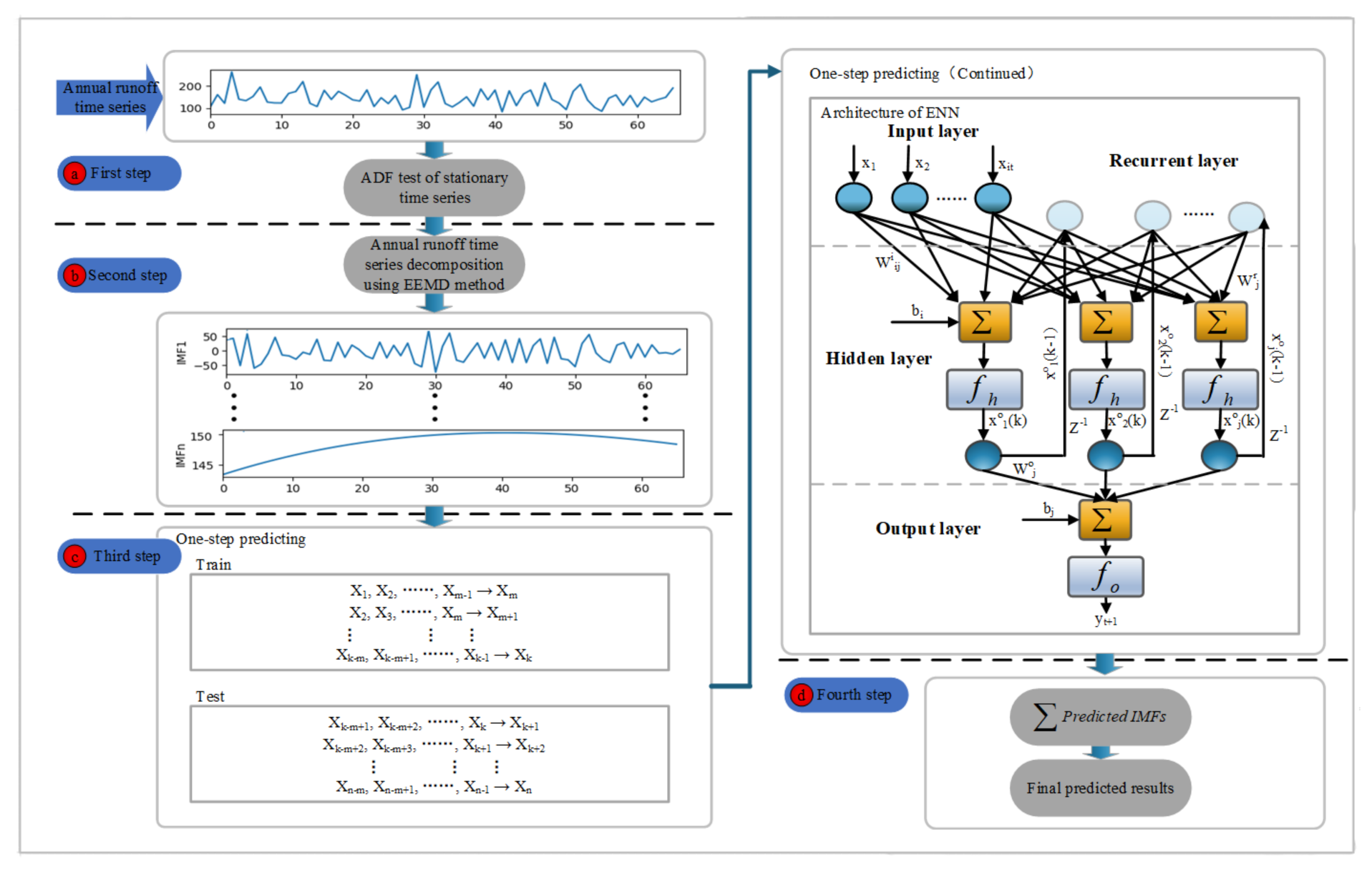
The Elman neural network (ENN), a member of the recurrent neural network family with global feedforward local network, was first proposed by Elman (1990) [37]. ENN consists of four layers, including an input layer, a hidden layer and a recurrent layer, which provide feedback from the outputs of the hidden layer to the hidden layer and the output layer. The addition of an internal feedback of the recurrent layer makes ENN more sensitive to historical data, increases the capacity to forecast the time series data and handles dynamic information, thus achieving the goal of dynamic modeling [38]. Therefore, it is suitable for modeling and predicting the annual runoff time series.

Further, the structure of ENN with multi-inputs and one output is shown in Figure 1 (upright) and can be expressed as the following formula:

$$x_{jt}^o\left(k\right)=f_h\left[{\displaystyle \sum }_{i=1}^m\left(w_{ij}^i{x}_{it}\left(k\right)+b_i\right)+{\displaystyle \sum }_{j=1}^n{w}_j^r{x}_{jt}^o\left(k-1\right)\right],$$

(4)

$$y_{t+1}\left(k\right)=f_o\left[{\displaystyle \sum }_j^m{w}_j^o{x}_{jt}\left(k\right)+b_j\right],$$

(5)

where $x_{it}$ ($i$ = 1, 2, 3, …, m) represents the input time series of neurons at time t. $x_{jt}^o$ ($j=1, 2, 3, \dots , n$) is the output of hidden layer neurons at time t. $y_{t+1}$ is the output of the network at time $t+1$. $w_{ij}^i$, $w_j^r$, $w_j^o$ are the weights that connect the nodes between input layer and hidden layer, between the recurrent layer and the hidden layer and between the hidden layer and the output layer, respectively. In addition, $b_i$ and $b_j$ denote the biases of the hidden layer and the output layer, whereas $f_h$ and $f_o$ are the transfer functions of the hidden layer and the output layer, respectively [39]. More details about the ENN can be found in Reference [40].

2.4. The Proposed Hybrid EEMD-ENN Model

Researchers had argued that hydrological time series data often shows different frequencies and complex nonlinear characteristics. Therefore, it is difficult to accurately model and predict using a simple model. Hence, a hybrid forecasting model based on EEMD and ENN—called EEMD-ENN—is proposed to improve the prediction accuracy of the annual runoff time series. The EEMD algorithm is utilized to decompose the annual runoff time series into several relatively stable IMFs and reduce the difficulty of modeling. Then, the IMFs are easily predicted by using ENN. Finally, the results of forecasted IMFs are aggregated as the final predicted results. Figure 2 clearly introduces the workflow chart of the proposed hybrid EEMD-ENN forecasting model in detail. The EEMD-ENN model contains four main steps as follows:

• First step: Nonstationary testing. To reveal, analyze and further study the nonstationary and nonlinear characteristics of annual runoff time series, the Augmented Dickey-Fuller (ADF) test is employed to analyze the stationary of annual runoff time series.
• Second step: Annual time series decomposing. The annual runoff time series are decomposed into several IMFs by using EEMD method.
• Third step: IMFs forecasting. One-step-ahead predicting is conducted for each IMF by using ENN. Several predicted IMFs results are achieved.
• Fourth step: Final predicted IMFs reconstructing. All the predicted results for every IMF are aggregated as the final predicted results for the annual runoff time series.

3. Case Study

3.1. Study Area

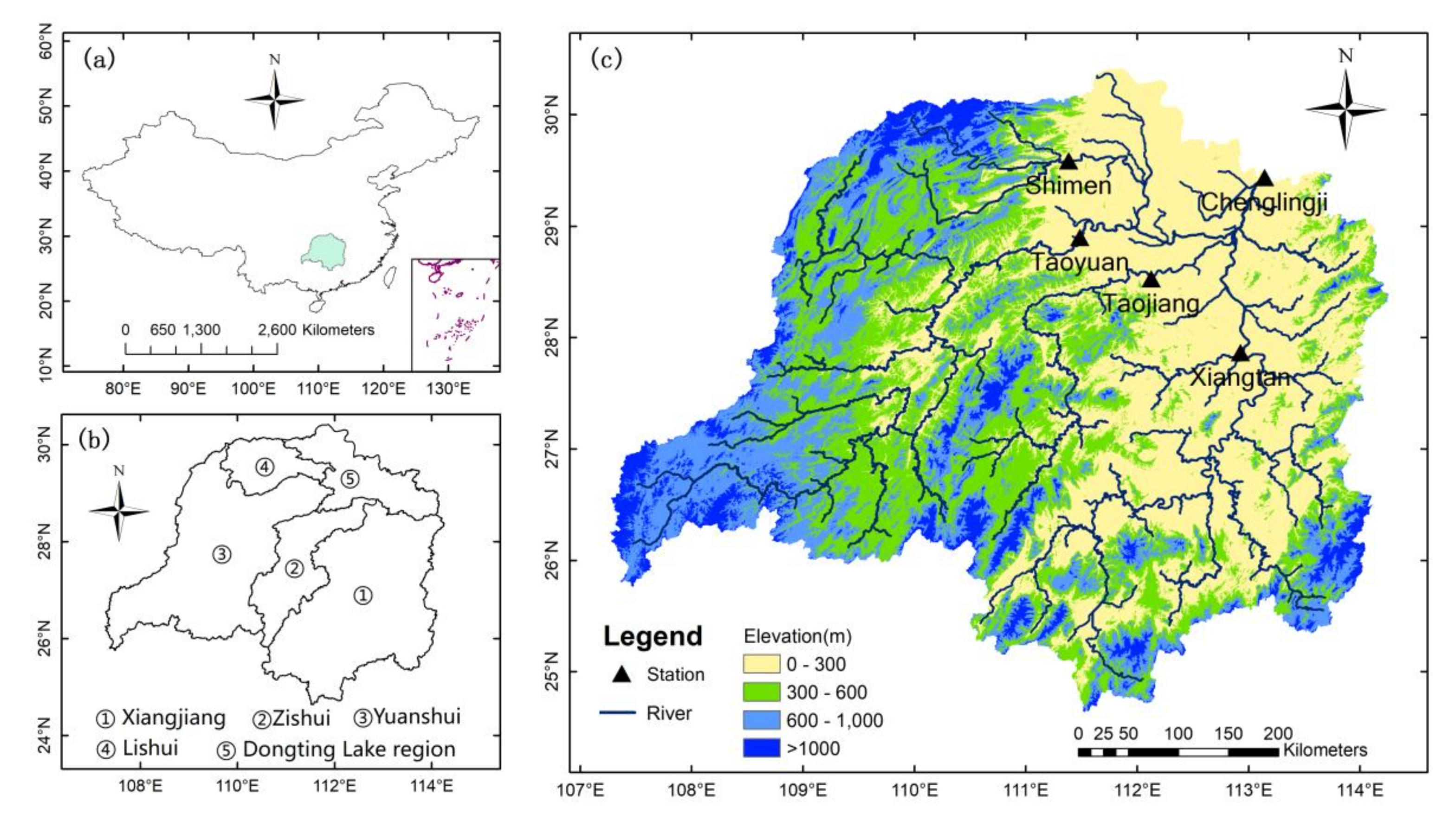
The Dongting Lake basin is located in the middle and lower reaches of the Yangtze River basin, in the central south of China and lies approximately between the longitude of 107°16′–114°15′ and the latitude of 24°38′–30°24′ (see Figure 2). It consists of four main rivers (Xiangjiang River, Zisui River, Yuanshui River and Lishui River) and flows through Guangxi, Guangzhou, Guizhou, Jiangxi, Hunan and Hubei, six provinces, discharging water into the Yangtze River through the Chenglingji outlet. The total drainage area of the Dongting Lake basin is 26.3 × 10⁴ km², accounting for 14.6% of the total drainage area of the Yangtze River basin [41]. From southwest to northeast, the topography of the basin varies from high mountains in the southwest and hilly areas in the center to the alluvial plains in the northeast (the lower reach of the basin) (Figure 2). The basin is in a subtropical humid monsoon climate zone with annual precipitation from approximately 1300 mm to 1800 mm and an annual mean temperature ranging from 16 °C to 18 °C [41]. Because of the low latitudes and geographical conditions, the sources of runoff are mainly supplied by rain and groundwater.

3.2. Data Collection

In this study, annual runoff data at five hydrological stations (i.e., Xiangtan station, Taojiang station, Taoyuan station, Shimen station and Chenglingji station) are selected as an example to demonstrate the modeling capabilities of the proposed hybrid EEMD-ENN model. The first four stations are the main controlling stations, located in the lower reaches of the four main rivers in the Dongting Lake basin, respectively and Chenglingji station is located at the outlet of the lake, central China (Figure 2). The annual runoff dataset for each station spanning from 1951 to 2016 were collected. The whole data set of the five stations are divided into two parts: the training data set and the test data set. The training data set covers runoff data from 1951 to 2003 and is used for building models, whereas the testing dataset covers runoff data from 2004 to 2016 and is used for evaluating the performance of the models. The annual runoff time series statistics are shown in

Table 1. Statistics of annual runoff time series.

Station	Period	Min. (108 m3)	Max. (108 m3)	Mean (108 m3)	Variance	Standard Deviation	Skewness	Kurtosis
Xiangtan	1951–2016 (Original dataset)	280.6	1031.9	654.5	27,120.48	164.68	0.24	2.45
	1951–2003 (Training)	280.6	1031.9	662.62	27,719.49	166.49	0.30	2.45
	2004–2016 (Testing)	358.2	873.1	621.44	25,309.80	159.09	−0.14	1.93
Taojiang	1951–2016 (Original dataset)	103.1	372.3	226.97	2545.16	50.45	0.51	3.72
	1951–2003 (Training)	103.1	372.3	231.59	2797.73	52.89	0.41	3.51
	2004–2016 (Testing)	149.2	266.3	208.16	1185.30	34.43	−0.07	1.95
Taoyuan	1951–2016 (Original dataset)	379.4	1030	643.51	15,285.81	123.64	0.42	3.1
	1951–2003 (Training)	454	1030	649.35	14,860.84	121.91	0.59	3.22
	2004–2016 (Testing)	379.4	822.7	619.73	17,638.21	132.81	−0.08	2.21
Shimen	1951–2016 (Original dataset)	82.98	264	146.54	1533.31	39.16	0.76	3.35
	1951–2003 (Training)	82.98	264	149.29	1691.78	41.13	0.71	3.05
	2004–2016 (Testing)	85.35	190.7	135.33	804.74	28.37	0.001	2.58
Chenglingji	1951–2016 (Original dataset)	1475	5268	2846.04	379,561.32	616.09	1.00	5.45
	1951–2003 (Training)	1990	5268	2960.01	362,336.39	601.95	1.19	5.59
	2004–2016 (Testing)	1475	3119	2381.38	194,570.92	441.10	−0.24	2.66

. The runoff data show high positive skewness and kurtosis.

3.3. Evaluation Indexes for Forecasting Performance

To evaluate the performance of the proposed hybrid EEMD-ENN model, the five main statistical indices are used as the evaluation indicators in this study, which have been widely and commonly used for evaluating the performance of hydrological simulation and hydroclimate models.

Firstly, mean absolute error (MAE), as one of the commonly used statistical indices, is used for measuring the average magnitude of the error between predicted data and observed data. The smaller the MAE value indicates better performance of the models. It is defined by the following formula:

$$MAE=\frac{1}{n}{\displaystyle \sum }_{i=1}^n\left|R_i^o-R_i^p\right|,$$

(6)

Secondly, mean absolute percentage error (MAPE) is a most frequently used statistics index and employed for examining the error between predicted data and observed data. It is defined by the following formula:

$$MAPE=\frac{1}{n}{\displaystyle \sum }_{i=1}^n\left|\frac{R_i^o-R_i^p}{R_i^o}\right|\times 100\%,$$

(7)

Thirdly, root mean square error (RMSE) is chosen as an evaluation index to test the differences between predicted data and observed data. The smaller of the RMSE value is, the closer the predicted data are to the observed data. It is defined by the following formula:

$$RMSE=\sqrt{\frac{1}{n}{\displaystyle \sum }_{i=1}^n{\left(R_i^o-R_i^p\right)}^2},$$

(8)

Fourthly, Pearson correlation coefficient (R) has been commonly and widely utilized for evaluating hydrological simulations and hydro-climate models. It assesses the degree of the co-linearity criterion between the predicted data and the observed data. The value of R is between −1 and 1. If the value of R is closer to zero, it indicates that there has been a weak or no linear correlation. In contrast, if R moves closer to −1 or 1, it denotes a perfect negative or positive linear correlation, respectively. The formula of R is defined as follows:

$$R=\frac{{\sum }_{i=1}^n\left(R_i^o-\overline{R^o}\right)\left(R_i^p-\overline{R^p}\right)}{\sqrt{{\sum }_{i=1}^n{\left(R_i^o-\overline{R^o}\right)}^2}\sqrt{{\sum }_{i=1}^n{\left(R_i^p-\overline{R^p}\right)}^2}},$$

(9)

Finally, the Nash–Sutcliffe coefficient of efficiency (NSCE) is a powerful and popular evaluation index for evaluating the performance of hydro-climate models. It was proposed by Nash and Sutcliffe [42]. NSCE range from 1 (best fit) to −$\infty$. If NSCE is close to 1, it indicates that the model performance is good and the model credibility is high; if NSCE is close to 0, it indicates that the predicted results are close to the average of the observed data, that is, the overall results are credible but the error of process prediction is large; while NSCE is much less than 0, the model is not trustworthy. It can be expressed as the following formula:

$$NSCE=1-\frac{{\sum }_{i=1}^n{\left(R_i^o-R_i^p\right)}^2}{{\sum }_{i=1}^n{\left(R_i^o-\overline{R^o}\right)}^2},$$

(10)

where n is the number of data points. $R_i^o$ represent the observed annual runoff time series at time $i$, while $R_i^p$ is the predicted annual runoff time series at time $i$. $\overline{R^o}$ denotes the average value of the observed annual runoff time series, whereas $\overline{R^p}$ stands for the average value of the predicted annual runoff time series.

3.4. Annual Runoff Time Series Decomposition by EEMD

To examine the nonstationary and nonlinear characteristics of annual runoff time series, the five original runoff time series are tested by using the ADF method. The results of ADF test are shown in

Table 2. ADF test results of annual runoff time series.

Station	h	p-Value	t-Value	Critical Value
Xiangtan	0	0.1952	−1.2402	−1.9454
Taojiang	0	0.2679	−1.0391	−1.9454
Taoyuan	0	0.3553	−0.8001	−1.9454
Shimen	0	0.1332	−1.4624	−1.9454
Chenglingji	0	0.2825	−0.9993	−1.9454

Notes: If the values of h equal to 1 indicate rejection of the unit-root null in favor of the alternative model, while the values of h equal to 0 indicate a failure to reject the unit-root null. If p-value greater than 0.05 and the t-value is greater than the critical value, this means the test result is not significant and would failure reject the hypothesis. Here, the significance level is set to 0.05.

. As seen in Table 2, the values of h equal 0, all the p-values are greater than 0.05 and all the t-values are greater than the corresponding critical values; this indicates that all the five annual runoff time series have unit-root and show strong nonstationary and nonlinear characteristics. So, it is difficult to achieve good prediction accuracy using single models.

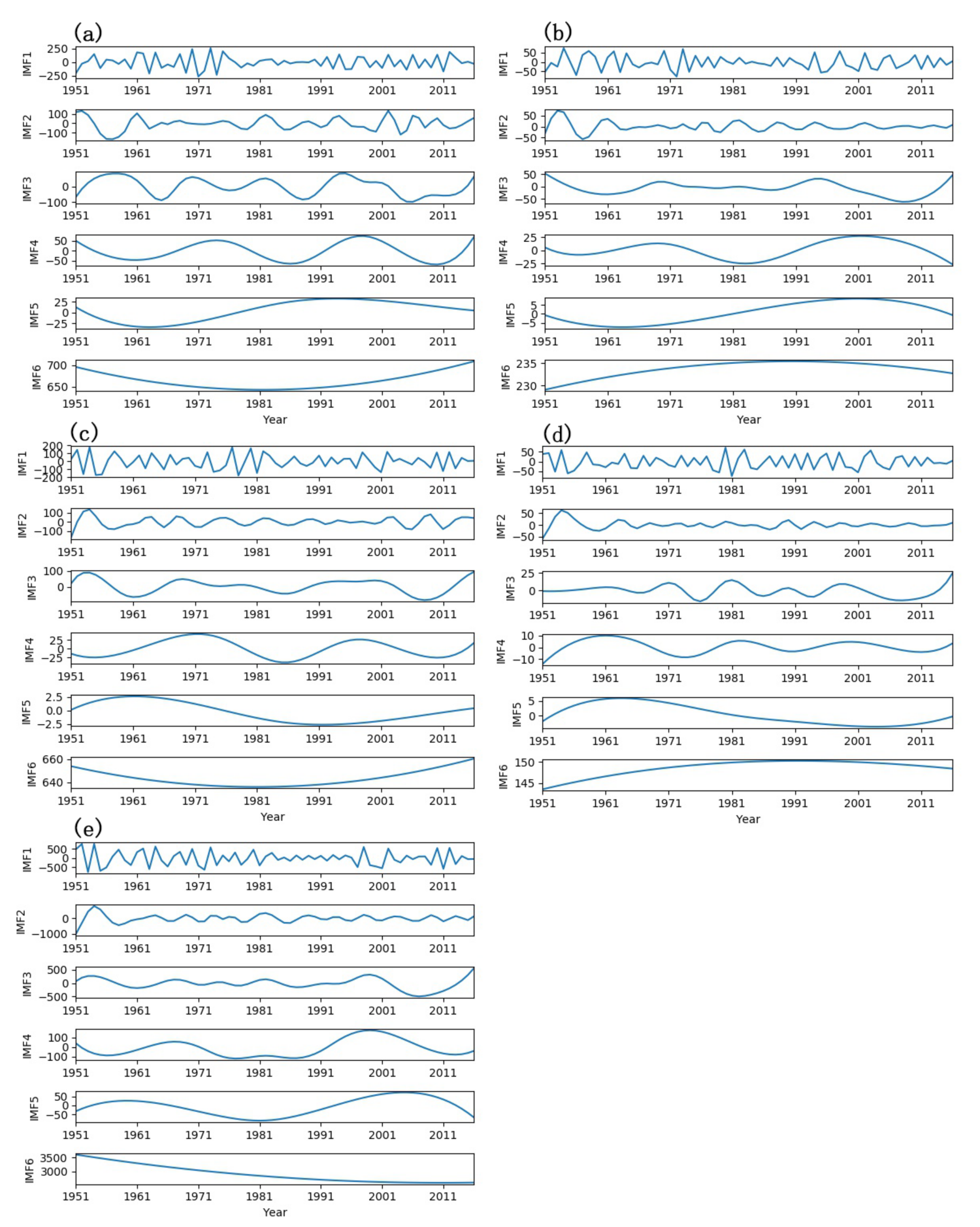
EEMD is a perfect method for nonstationary and nonlinear time series analysis, which decomposes the original time series to several relatively stable IMFs. In order to decompose the annual runoff time series, in this study, the ensemble number is set to 1000 and the amplitude of added noise is set to 0.2 times the standard deviation of the corresponding data [26]; several independent IMFs and a residual component (the last IMF) are obtained. The results are shown in Figure 3. As illustrated in Figure 3, the five annual runoff time series are decomposed into six IMF components. Each IMF component reports the oscillation characteristics in the order from high frequency to low frequency at various time periods and the final residual component demonstrates the overall trend of the original annual runoff time series, respectively. The results show that IMF1 and IMF2 of the five annual runoff time series exhibit 3 years and 5–8 years periodic fluctuation respectively, and IMF3 of the annual time series of Xiangtan station, Shimen station and Chenglingji station and Taojiang station and Taoyuan station shows 12–14 years and 17–20 years periodic fluctuation, respectively, and IMF4 of the five stations demonstrates 19–27 years periodic oscillation, while IMF 5 of Chenglingji station and other stations display 33 years and 62–64 years periodic oscillation, respectively. So, the EEMD method can be available and useful for decomposing nonstationary and nonlinear annual runoff time series to a relatively stable time series to improve the predicting precision.

3.5. Forecasting Each Intrinsic Mode Functions (IMF) Component and Reconstruction

After the decomposition of the original annual runoff time series into six IMFs by employing the EEMD method, we use the ENN model with three-layers to train and predict each IMF component. Here, one-step-ahead is used to predict the results, that is, five previous data points are used to predict the current one data point. The architecture of the three-layer ENN model for each IMF component is presented upright in Figure 1. The ENN model consists of one input layer with five inputs, for example, up to five previous ($x_{t-1}, x_{t-2}, x_{t-3}, x_{t-4}$ and $x_{t-5}$) values of each IMF component are set as the input data; one hidden layer including ten neurons; and one output layer having an output node, for example, $x_t$ value of the predicted results.

In this study, the tan-sigmoid is chosen as the transfer function from the input layer to the hidden layer, while the purelin function is selected as the transfer function from the hidden layer to the output layer [43]. The epoch for the training period is set to 5000 and in each training iteration the RMSE is adopted as the criteria for determining the optimum performance results. Before training the ENN model, all the values of IMFs are normalized to improve the efficiency of the ENN model. The normalization formula is defined as follows:

$$R_{nor}=\frac{R-R_{min}}{\left(R_{max}-R_{min}\right)\times \left(b-a\right)}+a,$$

(11)

where $R$, $R_{min}$ and $R_{max}$ represent the original, minimum and maximum value of annual runoff time series, respectively, $R_{nor}$ is the normalized annual runoff, whereas $a$ and $b$ denote the normalized in the range of $a$ and $b$. In the present study, the normalized value is set to the range from −1 to 1.

Finally, the predicted results of each IMF component are obtained and the predicted results of each IMF component are aggregated as the final prediction results of the original annual runoff time series.

3.6. Analysis and Performance Comparison

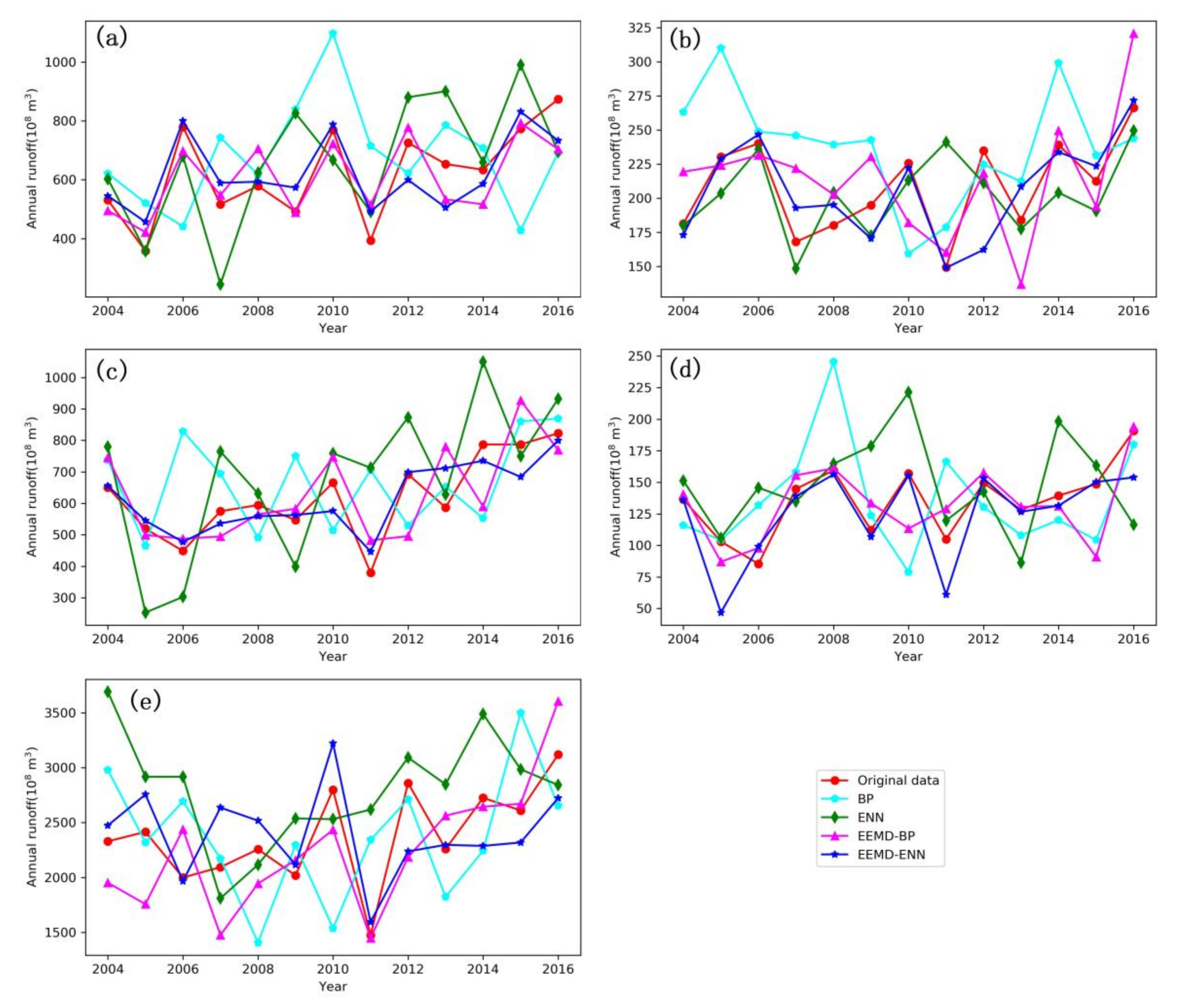
In order to understand the performance of the proposed hybrid EEMD-ENN model, the predicted results of the hybrid EEMD-ENN model are compared with the BP, EEMD-BP and ENN models. The predicted results of the four models are illustrated in Figure 4. It can be seen from Figure 4 that the BP, EEMD-BP, ENN and EEMD-ENN models give different forecast results for the five annual runoff time series. It is evident that the BP model, compared to the other three models, gives the worst results for the Xiangtan, Taojiang, Taoyuan and Chenglingji stations. The hybrid EEMD-BP and EEMD-ENN models perform better than the single BP and ENN models for the five stations but EEMD-ENN is slightly better than EEMD-BP at predicting the annual runoff time series for the five stations.

To measure the prediction performance of EEMD-ENN models, six evaluation indexes are adopted. They are MAE, MAPE, RMSE, R and NSCE. The statistical results of the four models are given in

Table 3. Prediction results comparison of ENN and EEMD-ENN models.

Station	Mode	MAE (108 m3)	MAPE (%)	RMSE (108 m3)	R	NSCE
Xiangtan	BP	206.79	62,027.17	235.17	0.002	−1.36
	ENN	141.82	62,035.71	172.40	0.59 *	−0.27
	EEMD-BP	75.91	62,043.40	90.13	0.81 **	0.65
	EEMD-ENN	72.12	62,040.99	85.65	0.83 **	0.69
Taojiang	BP	45.45	20,699.68	52.36	0.32	−1.51
	ENN	23.58	20,717.12	32.09	0.47	0.06
	EEMD-BP	28.13	20,712.44	32.92	0.66 *	0.18
	EEMD-ENN	15.61	20,716.65	24.18	0.75 **	0.47
Taoyuan	BP	154.46	61,860.46	184.77	0.09	−1.10
	ENN	123.34	61,872.48	145.33	0.43	−0.30
	EEMD-BP	97.22	61,870.23	115.70	0.64 *	0.18
	EEMD-ENN	47.46	61,872.61	59.99	0.89 **	0.78
Shimen	BP	33.28	13,429.19	42.44	0.29	−1.43
	ENN	33.48	3419.55	42.76	0.20	−1.46
	EEMD-BP	16.48	13,433.51	23.17	0.67 *	0.28
	EEMD-ENN	14.00	13,441.56	22.88	0.82 **	0.30
Chenglingji	BP	553.40	23,803.62	651.45	0.13	−1.36
	ENN	567.08	238,017.94	673.54	0.33	−1.53
	EEMD-BP	349.40	23,804.37	410.83	0.51 *	0.06
	EEMD-ENN	288.16	238,036.61	342.40	0.65 **	0.35

Notes: * indicates significant at the 0.05 level and ** indicates significant at the 0.01 level.

. According to the comparison between the BP, EEMD-BP, ENN and EEMD-ENN models, it is evident from Table 3 that the BP model has the worst results. The reason for the poor performance the BP model is the drawback itself, while the EEMD-ENN model performs better than the other three models. Moreover, the hybrid EEMD-ENN achieves smaller MAE, MAPE and RSME values than the EEMD-BP model and the single BP and ENN models, as well as the largest R and NSCE values for annual time series forecasting at the five stations. Furthermore, the R values of EEMD-BP and EEMD-ENN are significant at a confidence level of 0.05 and 0.01, respectively. Thus, the NSCE values of EEMD-BP and EEMD-ENN are greater than 0, this indicate that the predicted results of the two hybrid models are close to the average of the original annual time series, that is, the overall results are credible but the error of process prediction is large, while the NSCE values of EEMD-ENN model are great than EEMD-BP and are closer to 1, this indicates that the hybrid EEMD-ENN model is superior to the EEMD-BP model and is a suitable model for predicting annual runoff time series. In addition, from the comparison between the five stations, all the four models have poor performance for Shimen and Chenglingji stations. The possible reason is that the degree of dispersion of the training and testing data set at Shimen and Chenglingji stations is larger than that of the other stations (see Table 1) and another possible reason for this is that the skewness and kurtosis values are larger than for the other stations. This may lead to models facing difficulties in forecasting the annual runoff time series.

Depending on the aforementioned analysis, it is concluded that using the EEMD method to decompose the original annual runoff time series as the input data for the ENN model can, to a large extent, improve prediction precision. Therefore, the proposed hybrid model, based on EEMD and ENN, is the best model compared with the BP, EEMD-BP and ENN models and can achieve better forecasting results with significant improvement on the basis of five statistical evaluation indexes for predicting annual runoff time series.

4. Conclusions

In order to improve the prediction precision of annual runoff time series, we proposed a hybrid prediction model based on EEMD and three-layer ENN methods in this study and the hybrid model is applied to the annual runoff time series of the four hydrological stations (i.e., Xiangtan station, Taojiang station, Taoyuan station and Shimen station) in the lower reach of four main rivers in the Dongting Lake basin and one (i.e., Chenglingji station) at the outlet of the lake, central China. The main conclusions of this study are as follows:

Firstly, the results of the ADF test demonstrate that the original annual runoff time series from the five hydrological stations show strong nonstationary and nonlinear characteristics.

Secondly, the original annual runoff time series are decomposed into six stable IMFs to reduce the difficulty of modeling and improving the prediction accuracy. And then, all IMFs are divided into two parts: training data set and testing data set. Next, ENN has the capability for nonlinear modeling and is adopted to predict every IMF component. Finally, the predicted results of each IMF component are obtained and aggregated as the final prediction of the original annual runoff time series.

Finally, five statistical evaluation indexes (i.e., MAE, MAPE, RMSE, R and NSCE) are employed to measure the performance of the BP, EEMD-BP, ENN and EEMD-ENN models. The performance comparison of their prediction results in the present study demonstrates that the smaller values of MAE, MAPE and RMSE indicate the high prediction precision of the hybrid EEMD-ENN model. The higher values of R and NSCE demonstrate that the proposed hybrid EEMD-ENN model gives a better performance than the BP, EEMD-BP and ENN models.

The proposed hybrid EEMD-ENN model obtained a good prediction result for the five example study stations in our study but there are drawbacks, such as the number of neurons in the hidden layer were determined by human and no optimization algorithm was used to optimize the weights and biases of the ENN. In our future studies, we will determine the number of optimal hidden layer neurons through the ENN itself by changing the neurons dynamically and we will consider an optimization algorithm, such as the commonly used genetic algorithm (GA), particle swarm optimization (PSO) and gravitational search algorithm (GSA), to optimize the weights and biases of the network; and will apply this hybrid model to other river basins in mainland China. In short, the developed hybrid model can provide a significant improvement to annual runoff time series prediction.

References

- Zhang, Q.; Wang, B.-D.; He, B.; Peng, Y.; Ren, M.-L. Singular spectrum analysis and arima hybrid model for annual runoff forecasting. Water Resour. Manag. 2011, 25, 2683–2703. [Google Scholar] [CrossRef]
- Zhao, X.; Chen, X.; Xu, Y.; Xi, D.; Zhang, Y.; Zheng, X. An emd-based chaotic least squares support vector machine hybrid model for annual runoff forecasting. Water 2017, 9, 153. [Google Scholar] [CrossRef]
- Ning, L.; Xia, J.; Zhan, C.; Zhang, Y. Runoff of arid and semi-arid regions simulated and projected by CLM-DTVGM and its multi-scale fluctuations as revealed by EEMD analysis. J. Arid Land 2016, 8, 506–520. [Google Scholar] [CrossRef]
- Bao, A.-M.; Liu, H.-L.; Chen, X.; Pan, X.-L. The effect of estimating areal rainfall using self-similarity topography method on the simulation accuracy of runoff prediction. Hydrol. Process. 2011, 25, 3506–3512. [Google Scholar] [CrossRef]
- Bryant, A.C.; Painter, T.H.; Deems, J.S.; Bender, S.M. Impact of dust radiative forcing in snow on accuracy of operational runoff prediction in the upper Colorado river basin. Geophys. Res. Lett. 2013, 40, 3945–3949. [Google Scholar] [CrossRef]
- Erdal, H.I.; Karakurt, O. Advancing monthly streamflow prediction accuracy of cart models using ensemble learning paradigms. J. Hydrol. 2013, 477, 119–128. [Google Scholar] [CrossRef]
- Wang, W.-C.; Chau, K.-W.; Xu, D.-M.; Chen, X.-Y. Improving forecasting accuracy of annual runoff time series using ARIMA based on EEMD decomposition. Water Resour. Manag. 2015, 29, 2655–2675. [Google Scholar] [CrossRef]
- Wang, W.C.; Chau, K.W.; Qiu, L.; Chen, Y.B. Improving forecasting accuracy of medium and long-term runoff using artificial neural network based on EEMD decomposition. Environ. Res. 2015, 139, 46–54. [Google Scholar] [CrossRef] [PubMed]
- Chen, P.-C.; Wang, Y.-H.; You, G.J.-Y.; Wei, C.-C. Comparison of methods for non-stationary hydrologic frequency analysis: Case study using annual maximum daily precipitation in Taiwan. J. Hydrol. 2017, 545, 197–211. [Google Scholar] [CrossRef]
- Nijssen, B.; Lettenmaier, D.P.; Liang, X.; Wetzel, S.W.; Wood, E.F. Streamflow simulation for continental-scale river basins. Water Resour. Res. 1997, 33, 711–724. [Google Scholar] [CrossRef]
- Zhou, S.; Liang, X.; Chen, J.; Gong, P. An assessment of the VIC-3L hydrological model for the Yangtze River basin based on remote sensing: A case study of the Baohe river basin. Can. J. Remote Sens. 2014, 30, 840–853. [Google Scholar] [CrossRef]
- Srinivasan, R.; Ramanarayanan, T.S.; Arnold, J.G.; Bednarz, S.T. Large area hydrologic modeling and assessment part II: Model application. J. Am. Water Resour. Assoc. 1998, 34, 91–101. [Google Scholar] [CrossRef]
- Arnold, J.G.; Moriasi, D.N.; Gassman, P.W.; Abbaspour, K.C.; White, M.J.; Srinivasan, R.; Santhi, C.; Harmel, R.D.; Griensven, A.v.; Liew, M.W.V.; et al. SWAT: Model use, calibration and validation. Trans. ASABE 2012, 55, 1491–1508. [Google Scholar] [CrossRef]
- Liew, M.W.; Garbrecht, J. Hydrologic simulation of the little Washita river experimental watershed using swat. J. Am. Water Resour. Assoc. 2003, 39, 413–426. [Google Scholar] [CrossRef]
- Lin, K.; Zhang, Q.; Chen, X. An evaluation of impacts of DEM resolution and parameter correlation on TOPMODEL modeling uncertainty. J. Hydrol. 2010, 394, 370–383. [Google Scholar] [CrossRef]
- Devia, G.K.; Ganasri, B.P.; Dwarakish, G.S. A review on hydrological models. Aquat. Procedia 2015, 4, 1001–1007. [Google Scholar] [CrossRef]
- Zhao, X.-H.; Chen, X. Auto regressive and ensemble empirical mode decomposition hybrid model for annual runoff forecasting. Water Resour. Manag. 2015, 29, 2913–2926. [Google Scholar] [CrossRef]
- Wu, C.L.; Chau, K.W.; Li, Y.S. Methods to improve neural network performance in daily flows prediction. J. Hydrol. 2009, 372, 80–93. [Google Scholar] [CrossRef]
- Wu, C.L.; Chau, K.W.; Fan, C. Prediction of rainfall time series using modular artificial neural networks coupled with data-preprocessing techniques. J. Hydrol. 2010, 389, 146–167. [Google Scholar] [CrossRef]
- Taormina, R.; Chau, K.-W. Data-driven input variable selection for rainfall–runoff modeling using binary-coded particle swarm optimization and extreme learning machines. J. Hydrol. 2015, 529, 1617–1632. [Google Scholar] [CrossRef]
- Chau, K.W.; Wu, C.L. A hybrid model coupled with singular spectrum analysis for daily rainfall prediction. J. Hydroinform. 2010, 12, 458–473. [Google Scholar] [CrossRef]
- Humphrey, G.B.; Gibbs, M.S.; Dandy, G.C.; Maier, H.R. A hybrid approach to monthly streamflow forecasting: Integrating hydrological model outputs into a bayesian artificial neural network. J. Hydrol. 2016, 540, 623–640. [Google Scholar] [CrossRef]
- Wei, S.; Yang, H.; Song, J.; Abbaspour, K.; Xu, Z. A wavelet-neural network hybrid modelling approach for estimating and predicting river monthly flows. Hydrol. Sci. J. 2013, 58, 374–389. [Google Scholar] [CrossRef]
- Niu, W.-J.; Feng, Z.-K.; Cheng, C.-T.; Zhou, J.-Z. Forecasting daily runoff by extreme learning machine based on quantum-behaved particle swarm optimization. J. Hydrol. Eng. 2018, 23, 04018002. [Google Scholar] [CrossRef]
- Asadi, S.; Shahrabi, J.; Abbaszadeh, P.; Tabanmehr, S. A new hybrid artificial neural networks for rainfall–runoff process modeling. Neurocomputing 2013, 121, 470–480. [Google Scholar] [CrossRef]
- Wu, Z.; Huang, N.E. Ensemble empirical mode decomposition: A noise-assisted data analysis method. Adv. Adapt. Data Anal. 2009, 1, 1–41. [Google Scholar] [CrossRef]
- Huang, N.E.; Shen, Z.; Long, S.R.; Wu, M.C.; Shih, H.H.; Zheng, Q.; Yen, N.C.; Tung, C.C.; Liu, H.H. The empirical mode decomposition and the hilbert spectrum for nonlinear and non-stationary time series analysis. Proc. R. Soc. A Math. Phys. Eng. Sci. 1998, 454, 903–995. [Google Scholar] [CrossRef]
- Kang, A.; Tan, Q.; Yuan, X.; Lei, X.; Yuan, Y. Short-term wind speed prediction using EEMD-LSSVM model. Adv. Meteorol. 2017, 2017, 1–22. [Google Scholar] [CrossRef]
- Wang, C.; Zhang, H.L.; Fan, W.H.; Ma, P. A new chaotic time series hybrid prediction method of wind power based on EEMD-SE and full-parameters continued fraction. Energy 2017, 138, 977–990. [Google Scholar] [CrossRef]
- Niu, M.; Gan, K.; Sun, S.; Li, F. Application of decomposition-ensemble learning paradigm with phase space reconstruction for day-ahead PM2.5 concentration forecasting. J. Environ. Manag. 2017, 196, 110–118. [Google Scholar] [CrossRef] [PubMed]
- Zhang, N.; Lin, A.; Shang, P. Multidimensionalk-nearest neighbor model based on EEMD for financial time series forecasting. Phys. A Stat. Mech. Appl. 2017, 477, 161–173. [Google Scholar] [CrossRef]
- Lan, H.; Yin, H.; Hong, Y.-Y.; Wen, S.; Yu, D.C.; Cheng, P. Day-ahead spatio-temporal forecasting of solar irradiation along a navigation route. Appl. Energy 2018, 211, 15–27. [Google Scholar] [CrossRef]
- Ouyang, Q.; Lu, W.; Xin, X.; Zhang, Y.; Cheng, W.; Yu, T. Monthly rainfall forecasting using EEMD-SVR based on phase-space reconstruction. Water Resour. Manag. 2016, 30, 2311–2325. [Google Scholar] [CrossRef]
- Wang, W.-C.; Xu, D.-M.; Chau, K.-W.; Chen, S. Improved annual rainfall-runoff forecasting using PSO–SVM model based on EEMD. J. Hydroinform. 2013, 15, 1377–1390. [Google Scholar] [CrossRef]
- Barge, J.; Sharif, H. An ensemble empirical mode decomposition, self-organizing map and linear genetic programming approach for forecasting river streamflow. Water 2016, 8, 247. [Google Scholar] [CrossRef]
- Huang, N.E.; Shen, Z.; Long, S.R. A new view of nonlinear water waves: The hilbert spectrum. Annu. Rev. Fluid Mech. 1999, 31, 417–457. [Google Scholar] [CrossRef]
- Elman, J. Finding structure in time. Cognit. Sci. 1990, 14, 179–211. [Google Scholar] [CrossRef]
- Pan, Y.; Li, Y.; Ma, P.; Liang, D. New approach of friction model and identification for hydraulic system based on MAPSO-NMDS optimization Elman neural network. Adv. Mech. Eng. 2017, 9. [Google Scholar] [CrossRef]
- Ardalani-Farsa, M.; Zolfaghari, S. Chaotic time series prediction with residual analysis method using hybrid Elman–NARX neural networks. Neurocomputing 2010, 73, 2540–2553. [Google Scholar] [CrossRef]
- Kolanowski, K.; Świetlicka, A.; Kapela, R.; Pochmara, J.; Rybarczyk, A. Multisensor data fusion using Elman neural networks. Appl. Math. Comput. 2018, 319, 236–244. [Google Scholar] [CrossRef]
- Hayashi, S.; Murakami, S.; Xu, K.-Q.; Watanabe, M. Effect of the three gorges dam project on flood control in the Dongting Lake area, China, in a 1998-type flood. J. Hydro-Environ. Res. 2008, 2, 148–163. [Google Scholar] [CrossRef]
- Nash, J.E.; Sutcliffe, J.V. River flow forecasting through conceptual models part I—A discussion of principles. J. Hydrol. 1970, 10, 282–290. [Google Scholar] [CrossRef]
- Xu, J.; Chen, Y.; Bai, L.; Xu, Y. A hybrid model to simulate the annual runoff of the Kaidu River in northwest China. Hydrol. Earth Syst. Sci. 2016, 20, 1447–1457. [Google Scholar] [CrossRef]
Figure 1.
The flowchart of the proposed Ensemble EMD—Elman Neural Network (ENN) hybrid model for annual runoff time series forecasting.
Figure 2.
(a) location of Dongting Lake basin in central south China; (b) composition of the Lake basin and (c) the distribution of five hydrological stations.
Figure 3.
Decomposition of annual runoff time series of (a) Xiangtan station; (b) Taojiang station; (c) Taoyuan station; (d) Shimen station and (e) Chenglingji station.
Figure 4.
Performance comparison of the prediction results of the Back Propagation (BP), EEMD-BP, ENN and EEMD-ENN models. (a) Xiangtan station; (b) Taojiang station; (c) Taoyuan station; (d) Shimen station and (e) Chenglingji station.