Land Water-Storage Variability over West Africa: Inferences from Space-Borne Sensors


1
School of Earth Sciences and Engineering, Hohai University, Jiangning Campus, Nanjing 211100, China
2
State Key Laboratory of Hydrology-Water Resources and Hydraulic Engineering, Hohai University, Nanjing 210098, China
3
Department of Geomatic Engineering, Kwame Nkrumah University of Science and Technology, Private Mail Box, Kumasi AK000-AK911, Ghana
*
Author to whom correspondence should be addressed.
Water 2018, 10(4), 380; https://doi.org/10.3390/w10040380
Submission received: 22 December 2017
/
Revised: 13 March 2018
/
Accepted: 22 March 2018
/
Published: 25 March 2018
(This article belongs to the Special Issue Applications of Remote Sensing and GIS in Hydrology)
Abstract
:The potential of terrestrial water storage (TWS) inverted from Gravity Recovery and Climate Experiment (GRACE) measurements to investigate water variations and their response to droughts over the Volta, Niger, and Senegal Basins of West Africa was investigated. An altimetry-imagery approach was proposed to deduce the contribution of Lake Volta to TWS as “sensed” by GRACE. The results showed that from April 2002 to July 2016, Lake Volta contributed to approximately 8.8% of the water gain within the Volta Basin. As the signal spreads out far from the lake, it impacts both the Niger and Senegal Basins with 1.7% (at a significance level of 95%). This figure of 8.8% for the Volta Basin is approximately 20% of the values reported in previous works. Drought analysis based on GRACE-TWS (after removing the lake’s contribution) depicted below-normal conditions prevailing from 2002 to 2008. Wavelet analysis revealed that TWS changes (fluxes) and rainfall as well as vegetation index depicted a highly coupled relationship at the semi-annual to biennial periods, with common power covariance prevailing in the annual frequencies. While acknowledging that validation of the drought occurrence and severity based on GRACE-TWS is needed, we believe that our findings shall contribute to the water management over West Africa.
1. Introduction
There is ample evidence that West Africa (WA), which is home to about 290 million people inhabiting 18 countries, is facing a sustained reduction in its total rainfall amount [1]. For instance, Nicholson [2] reported that, although there has been an apparent resurgence in recent years, rainfall rates still remain well below those recorded in the first half of the 20th century. In addition, recent reports indicated that the freshwater flux, i.e., the difference between rainfall and evaporation, over WA is especially sensitive to rainfall fluctuations due to a long-term imbalance between the two fluxes [3]. These impacts on freshwater in WA have called for the analysis of the long-term and seasonal variability of rainfall, evaporation, and other hydrological variables to assess the availability and variability of freshwater over WA. Analyzing freshwater variability in WA is hampered by the fact that the region is data-deficient [4], so the required hydro-climatic information is not readily available. This makes it difficult to provide a more reliable account of the state of the region’s freshwater resources. Investigation of water storage variability has been limited to developed countries due to the availability of in-situ data and records, but even with that, the data is usually inaccessible or difficult to access. Fortunately, other data sources such as those observed from space-borne sensors can be employed to overcome the data scarcity in many poor-data regions worldwide.
To circumvent the problem of hydro-climatic data shortage, various studies have attempted to analyze and explain the variability of available freshwater in the context of runoffs and/or river discharge [1,5,6], rainfall patterns [7,8], vegetation dynamics [9,10], land water storage [11], etc. Nevertheless, the Gravity Recovery and Climate Experiment (GRACE) satellite mission has eased the quantification of land water storage in terms of data shortages. The mission provides the total water storage (hereafter abbreviated as TWS) from which the other components of the water cycle can be segregated if ancillary data are available [12,13]. Fluctuations of hydro-meteorological variables such as precipitation, evaporation, and stream flow are the basis of drought induction [14] and, as a consequence, based on hydrographs, have impacted land water storage. Thus, GRACE data has assisted in the quantification of hydrological processes, which are necessary for drought analysis. When dry conditions set in, hydrologic events, which feed the atmosphere with enough moisture for precipitation, establish positive feedback processes for a drought episode [14]. An atmosphere with depleted moisture has little relative humidity, hence lessening the probability of rainfall. Rainfall in such situations only occurs when moisture carrying winds from other regions provide enough humidity for precipitation [15].
In a review of droughts in the African continent, recent studies [16,17], mentioned that WA was one of the regions prone to droughts in the near future. This might be possible due to the rapid population growth and poor drought assessment methods in the region. Nevertheless, the most common studies involving the GRACE data over the WA have been based on the quantification of the water-storage variability and not the potential for drought characterization. For instance, Andam-Akorful et al. [8] assessed the water-storage variability of the whole of WA based on net-precipitation, while Ndehedehe et al. [18] explored the variation of hydrological droughts based on different precipitation indices together with water storage variability from GRACE. There are only a few studies on the potential of characterizing and quantifying droughts directly from GRACE-derived TWS on specific regional basin scales. For example, studies have focused on the Volta Basin [18,19,20,21], the Niger Basin [22], and the Senegal Basin [23]. For WA, GRACE-based drought characterization is uncommon. However, drought characterization based on the GRACE water storage deficits approach has been studied by Thomas et al. [24] for the Amazon and Zambezi River basins. This method has helped determine the duration and severity of drought events. Additionally, for the São Francisco River basin, Sun et al. [25] reported on drought characterization employing GRACE-derived storage indices.
Therefore, the main aim of this study was to analyze the terrestrial water storage (TWS) changes over WA as observed by GRACE. Our objectives were (1) to deduce the water mass gain of Lake Volta with respect to the major basins in the region, (2) to explore the potential of GRACE-derived TWS for hydrological drought characterization after considering the lake’s effect, and (3) to investigate the impacts of hydro-climatic variables on TWS changes. To achieve this, satellite altimetry and imagery datasets are combined to account for the surface water storage of Lake Volta, a significant reservoir in the region, from GRACE-derived TWS. Furthermore, we present a framework comparison involving co-variability studies of GRACE-derived terrestrial water-storage change (TWSC, the derivative of TWS w.r.t. the time) with precipitation (rainfall), the normalized difference vegetation index (NDVI), and the teleconnection index (El Niño Southern Oscillation—ENSO).
2. Materials and Methods
2.1. Study Area
2.1.1. Geography
West Africa refers to the geographic western part of the African continent, which is spread within the range of latitudes 0° to 20° N and longitudes 20° W to 20° E. The total area comprises of about 5,112,903 km2, which accounts for 20% of the total land area of the whole of Africa. The region is bordered by the Atlantic Ocean to both the west and the south, to the north by the Sahara Desert and to the east by two Central African countries, Chad and Cameroon (Figure 1). The main river basins in WA are the Niger, the Volta, and the Senegal. The Niger Basin is the largest, covering a total area of 1,926,905 km2 (excluding 9% of its area outside WA, located in Algeria and Chad). It accounts for about 37% of the total area of WA, while the Senegal and the Volta both occupy an area of 434,749 km2 and 412,481 km2, respectively, making up 8% of the total area of WA. In total, the three basins occupy about 54% of the entire sub region. We considered the main basins instead of the entire region to avoid suppressing inherent drought features in some regions of WA. Ndehedehe et al. [18] indicated that, considering the entirety of WA as a whole, such analyses may lead to the misrepresentation of areas with relatively lower drought signature amplitudes as insignificant, whereas they may be significant at a sub-regional scale.
An important feature in the region is Lake Volta, which, located in Ghana, is one of the largest manmade lakes in the world, due to the construction of the Akosombo Dam in 1964. It is located at a latitude of 6.5° N and a longitude of 0° W (Figure 1). As the largest lake in the basin, it contributes to the environmental, economic, and social activities of the country and the entire basin.
2.1.2. Climate
West Africa experiences unique climatic conditions of wet and dry seasons resulting from the exchange of two migrating air masses that prevail virtually across the entire region. They are hot and dry Harmattan winds that blow from the Sahara over the entire region from November to February and the tropical maritime or equatorial air mass, which produces counter southwest winds. The meeting point of these two air masses forms a belt of variable width and stability called the Intertropical Convergence Zone (ITCZ), which influences the climate of the region.
West Africa has four climatic zones: the arid zone (Sahelian), the semiarid zone (Sudanian), the sub-humid zone, and the humid zone (the equatorial) [8]. The Sahelian is the northern section forming the transition between the Sahara and savannah; rainfall in this area is irregular and does not exceed three months with less than 500 mm rainfall. In the Sudanian portion, precipitation is less than 88 mm in the north of Nigeria and 1000 mm in the north of Mali, whereas the tropical humid zones have an average rainfall of approximately 1500 mm.
2.2. Datasets
2.2.1. GRACE-TWS Monthly Fields
To assess the variability of water storage in WA, we employed GRACE-derived monthly TWS fields provided by NASA’s Jet Propulsion Laboratory (JPL) GRACE Tellus [26], otherwise known as Level 3 (L3) products. They are gridded mass estimates expressed in terms of monthly TWS fields at a spatial resolution of 1° (~111 km at the equator), which is much finer when compared to the nominal GRACE resolution (~333 km at the equator). The University of Texas Center for Space Research (CSR) version was acquired in this study since it has been proven to give the smallest uncertainties over the major river basins of WA [27]. Specifically, uncertainties of approximately 5.0, 6.0, and 5.9 mm have been estimated for Niger, Senegal, and Volta, respectively [27]. The TWS grids used in this study spanned the period from April 2002 to July 2016 with the fields for June 2003, January and June of 2011, and May and October of 2012 missing.
Compensation due to all the filtering processes and truncation of spherical harmonic coefficients (SHCs) was applied in terms of gain factors [26]. A gain factor k was derived by minimizing the discrepancies between the unfiltered true () and the filtered () storage time series, at each grid point, through a least square regression expressed as [26]
where is the unfiltered storage (“true” signal) and is the filtered storage after expansion to SHCs and filtered with the same filters as the GRACE. Global Land Data Assimilation System (GLDAS)-driven Community Land Model (CLM4.0) version 4 [28] was used to simulate the water storage time series, which are independent of the GRACE.
Apparently, this gain factor, when applied to the filtered GRACE data, restores a significant portion of the signal attenuation, and the resultant gridded TWS enhances data compatibility with other gridded datasets. For example, when comparing TWS data with rainfall, one does not have to filter the rainfall data as the GRACE. However, the quality of the resulting TWS depends on the quality of the simulated TWS. Models such as GLDAS CLM4.0 do not consider water management such as groundwater abstraction, surface water impoundment and division, etc. Thus, inter-annual trends could present large uncertainties, and the estimated scale factors using Equation (1) are dominated by annual cycles. A well-structured analysis of leakage restoration and scale factor application is further discussed in, for example, Ref. [29].
2.2.2. Bivariate ENSO Time Series
The Bivariate ENSO Time Series (BEST) is a climate index that characterizes the ENSO phenomenon. The ENSO is derived from the combined effect of Niño 3.4 and the Southern Oscillation Index (SOI). The BEST index was obtained for the period coinciding with the GRACE (that is, from April 2002 to July 2016).
2.2.3. Tropical Rainfall Measurement Mission Rainfall Products
The rainfall product employed was the Tropical Rainfall Measurement Mission (TRMM). TRMM was launched in November 1997 to operate for 3 years, and fortunately survived for nearly 17 years of effective data acquisition to study rainfall and climate research. It was a joint mission between National Aeronautics and Space Administration (NASA) and the Japan Aerospace Exploration (JAXA) to study tropical rainfall in the latitude range of ±50°. The monthly mean 3B43 V7 [30] rainfall rate products of a 0.25° spatial resolution were used in this study, and were compiled not only from TRMM but from other satellite products and ground-based rain gauge data as well [31]. The data were obtained from NASA’s Goddard Earth Sciences Data and Information Service Center (GES DISC). This dataset has been evaluated for several regions globally, for instance, for the whole of WA, as inferred by Nicholson [2] in the attempt to verify the recovery of rainfall in the region. Additionally, Forootan et al. [11] employed this dataset together with sea surface temperature (SST) data for the water storage deduction of WA. Furthermore, several studies [12,19,32,33] have employed this data over WA, and Awange et al. [34] reported that it performed quite well over Africa.
2.2.4. Satellite Altimetry Data
Satellite radar altimeters are basically designed to measure the world’s ocean and ice sheets. However, advanced manipulation of this data has enabled studies in water level variations and storage changes of large lakes, reservoirs, and wetlands at global scales [35]. Satellite altimeters are advantageous, in that they provide day and night observations with no cloud restrictions. Since 1992, the available satellite altimetry missions have been combined to routinely measure lake and reservoir height variations for many large lakes around the world in near real time. The satellite altimetry data used in this study were obtained from the U.S. Department of Agriculture’s Foreign Agricultural Service (USDA-FAS) in collaboration with NASA and the University of Maryland online database of global lake and reservoir measurements. However, this dataset has a temporal resolution of about 10 days; which was then filtered and resampled to a monthly time step. This data have also been used in other studies [11,19,20]. Validation of this dataset over some selected reservoirs globally including Lake Volta was evaluated in [36] whereas a root-mean-square-error (RMSE) of 0.54 m with a correlation coefficient of approximately 0.99 (95% confidence level) was obtained for Lake Volta. This RMSE is approximately 4 mm (4 kg/m2) in terms of water equivalent height over the basin estimated by the propagation of uncertainty.
2.2.5. Satellite Imagery Data
The MOD13Q1 NDVI data, acquired from the Land Process (LP) Distributive Active Archive Center (DAAC) of NASA and United States Geological Survey (USGS) was used in the study. The Global MOD13Q1 data are a gridded level-3 product in the sinusoidal projection, at spatial and temporal resolutions of 250 m and 16 days, respectively. It was considered due to its 250 m resolution, which is the least among the MODIS products. MODIS data are also cloud-free when compared to other datasets such as Landsat despite its coarse resolution [37]. Previously the MOD13Q1 has been used in Islam et al. [38] for flood inundation, and for surface area derivation by Gao et al. [39]. Additionally, the MODIS global vegetation index product MOD13C1 provides vegetation index classification systems. Furthermore, it provides a land cover type assessment, and quality control information. The MODIS Version 5 yearly land cover type L3, 500 m global sinusoidal data (MOD13C1) were obtained from NASA’s Land Data Products and Services (LP DAAC). This dataset was used to analyze the NDVI variations over the study area as well.
2.3. Methodology
2.3.1. Lake Surface Area and Height Changes
The most commonly used method for reservoir water storage estimation using remote sensing data is to extract water surface area and elevation separately, then, combine these two sets of information for storage calculation [37,39]. The water surface area was delineated from the MODIS13Q1 NDVI images (Section 2.2.5), while the water surface elevations were obtained from satellite altimetry (Section 2.2.4). For every month, one set of the 16-day 250 m product was acquired, which consisted of two scenes that covered the entire Lake Volta. Both scenes were mosaicked to form a single image and a further subset for the area of interest. Hence, a single image represented every month creating 12 images per year. From the period of April 2002 to July 2016, a total of 172 NDVI images were obtained. However, due to the poor quality of the images in some months due to cloud cover, 110 months of the best image quality were used out of the 172 images.
A mask was created to separate the water pixels from land using a given threshold. The NDVI values ranged from −1 to +1 with water values mostly being less than zero. The threshold was manually adjusted for every image and then compared with the true color image to avoid misclassifications. This method is similar to those used by Wang et al. [40] and Sheng et al. [41]. Basically, the range of values for each image was found considering the values for the middle of the lake and outside the lake as land or non-water. The mask was then applied, the images were converted to binary images containing pixels 1 for water and 0 for land and vegetation.
The binary images were further converted into shapefiles, delineating the shape of the lake and extracting the lake shorelines. The coordinates of the lake were then used to compute the corresponding monthly surface area in square kilometers (km2). This procedure was used to process every image separately due to the different acquisition dates.
To predict the surface area of the missing months of the overall period, an area–elevation relationship was derived such that either parameter could be inferred from its pair where the direct observation was unavailable as described in [37]. Due to the correlation of the known elevations and surface areas, a linear polynomial was chosen to describe the area–elevation relationship (Section 3.1.1).
2.3.2. Lake-Induced TWS Changes
At this point, the lake boundary obtained was combined with the lake height changes to deduce the contribution of Lake Volta. However, these data were converted into SHCs and filtered with the same filtering scheme as the GRACE data to enhance data compatibility in the spectral domain. It was necessary to have the data in the same resolution (spectral). To accomplish this, a global grid mask was constructed by a kernel function using the spherical coordinates of the lake extent [42]:
where is the co-latitude and is the longitude. This global grid mask could be, for example, constructed/achieved at grid intervals of to adequately capture the lake’s shape [20]. Using the spherical harmonic analysis, a grid integral function on a sphere can be analyzed into SHCs, and , as [42]
where , and is the normalized associated Legendre function of degree and order m. The spherical harmonic synthesis using the coefficients from Equation (3) can then be used to reconstruct the lake’s shape [42]:
To deduce the altimetry-derived TWS of the lake, a standard shape of the lake was chosen and used together with the monthly shape variations of the lake to scale the altimetry time series. To this end, it was proposed to compute the area of the standard shape as using its boundary coordinates, and this standard shape was then expressed in terms of SHCs using Equation (3). The advantage of this procedure is that there was no need to expand each monthly shape of Lake Volta obtained from the satellite imagery since there were missing months; consequently, this reduced numerical computational time required to compute the coefficients in Equation (3). Furthermore, this procedure was more sensitive to the lake’s areal changes relatively to an expansion in SHCs of each monthly shape. Thus, the following expression was proposed here and could be used to compute the altimetry/imagery derived TWS fields:
where is the altimetry-derived TWS due to Lake Volta’s water impoundment; is the monthly surface area of the lake; is the satellite altimetry height, is the month, and is the standard area of lake. Here, it was considered as the standard shape the one that has been widely used in many GRACE applications over the Volta Basin. This shape was provided with an area of about 8500 km2, as reported by many authors and produced by the Digital Chart of the World (DCW).
The averaged values of the can be extracted over the regional basins, considering the major basins in WA (the Volta, the Niger, and the Senegal). The regional average of any gridded quantity within any given region such as a basin or a lake can be computed as [19]
where is the number of cells within a basin (or a region); is the area of the cell ; is the total area of the basin. (For this study, the cell size was 1° × 1°.) Finding the average over each basin determines the contribution of the lake in each basin, respectively. This was used to determine the contribution of Lake Volta’s impoundment on the TWS of each basin.
2.3.3. Droughts Characterization
Studies such as Sun et al. [25] and Thomas et al. [24] have confirmed TWS as a more dependable means for drought analysis, since it reflects all the combined factors of hydrological changes including human effects. However, the GRACE-derived TWS time series did not cover the desired 30-year period. Thus, to compute the droughts, a normal condition based on “quasi-climatology” (mid-term climatology) was considered using the median for computing the monthly normals. Originally, this approach was based on the mean, but the median was used due to its robustness to extreme values. The normals are a long-term seasonal measure of the average water storage that exhibits the standard trend of storage variability. Therefore, it serves as the reference or the baseline for identifying the occurrence and severity of droughts. Hence, positive deviation from the standard (climatology) indicates excess water, while negative deviation indicates water loss, deficits, or dry conditions.
These deficits or gains give a straightforward measure of the magnitude M (km3), in other words, the volumetric difference from the standard hydrological conditions (normals), so the volume of water needed to return to normal conditions. Finally, a drought “event” was concluded to have occurred if the magnitude M below-normal conditions occurred consecutively for a period of 3 months or more. This allowed for event-based classification and comparison. To assess the cumulative impact of the water storage deficit and duration (3 consecutive months or more), a severity term S was defined with respect to time. The severity of the drought conditions (S) can be obtained by multiplying the average deficit by the duration, which can be expressed as [24]
where is the average deficit for all drought events, is the specific month, and D is the duration.
This storage-based approach is beneficial as it provides a means of estimating the drought recovery using the deficits, since the monthly deficit (M) is the quantity of water required to recover from below-normal water storage conditions. Hence, the rate of change in the increase or decrease of the storage deficits can be deduced from the time derivatives of the deficits. By employing a backward difference calculation, the rate of change can be expressed as [24]
where M is the monthly deficit, and 𝑡 is the time. Due to the short time span of the GRACE data, drought occurrences might have been few in number. Thus, time series was presumed to be the entire set of values, including those in previous drought recoveries.
To estimate the minimum and maximum time to recovery for each drought epoch, the distribution and statistical percentiles of the values were computed. This was achieved by using the Lilliefors statistical test for normality based on the Kolmogorov–Smirnov test (KS-test). Based on this test, all three basins (Volta, Niger, and Senegal) followed a normal distribution. Hence the 68th percentile and the 95th percentile of the empirical Cumulative Distribution Function (eCDF) were used to obtain the minimum and average time to recovery for the deficits.
2.3.4. Cross Wavelet Transform and Coherence
Time series of hydrological datasets (such as rainfall or runoff) inherit some hidden properties that are of great significance. Techniques such as Fourier transforms assume them to be stationary in the frequency domain but they are variable in time [43]. Wavelet transformations, however, reveal the frequency trends of these datasets with respect to space and time dynamics [44]. Two forms of wavelet transforms are deduced; the continuous wavelet transform (CWT) and its discrete wavelet transforms (DWT). CWT is preferred for detail extraction, while the latter is better for compact data description and for noise reduction. CWT provides a representation of signals in a time scale. Linking two CWTs releases the associated similarities between two datasets, and this is known as cross wavelet transform (XWT). XWT produces the cross power and related frequency between the two datasets. Cross wavelet is a tool for analyzing the distribution among time series, and further coherence provides inherent coherence between the two signals datasets. In this study, the XWT and its coherence were used to analyze nonlinear time series data. For two distinct time series and , the XWT can be expressed as
where * is a complex conjugation. is the cross-wavelet power, which is defined as the magnitude, while the complex argument, arg(), reveals the local relative phase between the two given fields in the time frequency space.
In the same way, the coherence of the two time series can be shown as
where S is a smoothing operator, s is the wavelet scale, is the cross wavelet transform between the two CWTs, and and represent the two time series. Therefore, in this study, the inherent response and interactions between the GRACE-derived TWS and other climatic variables such as rainfall, BEST, and NDVI were analyzed.
3. Results
3.1. Altimetry-Imagery Infered TWS Variations (LakeTWS)
3.1.1. Lake Surface Area Changes
Following the processing of the MODIS images (Section 2.3.1), a set of surface area variation time series were deduced. A linear model was estimated using a simple least square regression to obtain the best fitting parameters between areal surface changes (satellite imagery) and water elevation (satellite altimetry) as shown in panel (a) of Figure 2. The best fit parameters were obtained as the slope c and the intercept m of the fitted least square regression line. The area–elevation relationship (i.e., y and x, respectively) for Lake Volta over the study period was estimated as
with a Pearson’s correlation coefficient () of approximately 0.89 showing high correlation between the surface area and altimetry heights (panel (a) of Figure 2). The area–elevation relationship in Equation (11) was then used for making provisions for the missing months of MODIS data as described in Section 2.3.1. Figure 2 also shows the surface area, lake water level, and volume variations obtained for the entire study period.
The peak surface area for the entire period was recorded in November 2010 as 9194 km2 corresponding to a height change of 7.4 m, while the minimum surface area was 4693 km2 with a height of −3.2 m (Figure 2). An average surface area of 6800 km2 was obtained—not 8500 km2 as reported by numerous authors [45,46,47]. Furthermore, this range of surface area values obtained here for Lake Volta (4690 and 9190 km2) conformed with the results of Tanaka et al. [48] in their attempt to obtain the surface area of Lake Volta from DMSP-SSMA (Defense Meteorological Satellite Program-Special Sensor Microwave/Imager) data. Their results ranged from 4450 to 9970 km2, affirming the further conclusion that the surface area of 8500 km2 was unrealistic. This might have led to the overestimation of the resulting storage when combined with altimetry data in next Section 3.1.2.
Noteworthy, one could use only the satellite imagery data and any available digital elevation model (DEM) for extracting the lake elevation at each image epoch relative to the DEM’s datum. For example, Tanaka et al. [48] have overestimated the parameters of the area–elevation relationship in 44.9% relative to the values found in this study. Such an approach would be more interesting since it would also allow for an estimation of river bed changes when large flows are introduced. Unfortunately, there is no accurate DEM available for the public domain at present [49]. Thus, this shall be carried out in the future.
3.1.2. Lake Kernel Function
Lake kernel function is essential to scale the altimetry-imagery-derived TWS of the lake for spectrally consistency with the GRACE data. Thus, it is essential for data compatibility. For Lake Volta, the kernel averaging method [42] has also been applied in studies such as [19,20] to synthesize the altimetry-derived storage of the lake. The averaging lake kernel functions expressed in terms of SHCs as ones inside the lake and zeros anywhere else (see Equations (2) and (3)) were computed at different spatial resolutions (Figure 3). This was necessary to verify the absolute kernel resolution desirable for the kernel function to capture the irregular shape within the lake as suggested in [20]. Nevertheless, it is quite significant to note that kernel function amplitudes differ for different resolutions and can also be the same amplitude for different resolutions (Figure 3).
Apparently, the kernel function at a coarse spatial resolution of 0.5 arc-degree provides an associated maximum amplitude, shown on the color bar above 0.03 in Figure 3a. However, the associated function amplitude corresponding to the 0.1 arc-degree (Figure 3b), 0.05 arc-degree (Figure 3c), and 0.00833 arc-degree (Figure 3d) in all exhibited the same kernel function amplitude around approximately 0.03. Hence, the coarsest and the smoothest resolutions from Figure 3a,d had significant amplitude differences; therefore, the least resolution, 0.00833 arc-degree (30 arc seconds), was chosen. Next, it was then passed through with the same filter scheme as applied to the GRACE, i.e., the polynomial filter and the Gaussian 300 km half-width pass filter. Figure 4a shows the 30 arc-seconds kernel after applying the half width filter and the polynomial filter. Application of these filters reduces the amplitudes of the kernel and spreads out of Lake Volta’s domain. Figure 4b also shows the ratio between the lake kernel filtered as shown in Figure 4a and the kernel displayed in Figure 3d.
Since the GRACE gridded dataset is at a 1 arc-degree resolution, it was necessary to compute a kernel grid of the same resolution to enhance data compatibility in the space domain using Equation (4). Then, at each grid point with a resolution of 1° × 1° was used to compute (TWS of Lake Volta) fields as per Equation (5). The results are presented in Figure 5 in terms of linear rates (panel a) and root-mean-square (RMS) (panel b). The RMS shown in Figure 5b depicts the strength of the seasonal water level variations of Lake Volta over WA as “sensed” by GRACE.
The time series of LakeTWS for the Niger, Senegal and Volta Basins were averaged using Equation (6), respectively. Next, their linear trends were estimated. The results in this study revealed an overall regional trend of 0.63 ± 0.14 mm/year for the Volta, 0.06 ± 0.01 mm/year for the Niger, and 0.08 ± 0.02 mm/year for Senegal. It is noteworthy that the RMSE estimated for the altimetry data (Section 2.2.4) was based on water measurements, which is equivalent to approximately 4 mm spread over the Volta Basin (without considering the SHCs of the lake’s shape). Considering the rates of LakeTWS for the Volta Basin over the time window of 14.25 years, this would be equivalent to an accumulated water mass gain due to Lake Volta of about 9.0 mm, which is more than double the estimated altimetry error (4 mm). This provided confidence in using the derived altimetry series despite the large “uncertainty” for Lake Volta. We did not use this error when we estimated the linear rates of LakeTWS because it was estimated based on gauge data located at Akosombo Dam, which was different from the altimetry radar tracks. The best option would be to calibrate the altimetry missions over Lake Volta, and this might be carried out in the near future.
3.2. GRACE-Derived TWS Variations
The TWS obtained from GRACE is the sum of all the possible water compartments such as soil moisture, groundwater, reservoirs, and lakes [50]. To determine the actual TWS (irrespective of surface water) of a given region, it is necessary to acquire an idea of the contribution of significant surface water bodies (reservoirs and lakes). Seasonal fluctuations and climate change effects on these lakes and reservoirs have an impact on the TWS of a region, which might result in the overestimation of the GRACE-derived water storage [47,50], which is important to consider in drought characterization. Figure 6 (panels a and b) shows the spatial map of TWS (total TWS with all components) computed from April 2002 to July 2016 without the scale factor applied (panel a) and with the scale factor applied (panel b), respectively. (Scale factor has been addressed in Section 2.2.1.)
As seen in Figure 6a, low rates of TWS were observed due to the signal loss from the application of filtering processes and leakage effects; however, the linear rates increased in Figure 6b after the application of the GLDAS CLM 4 scale factor, indicating that there had been some amount of restoration of the loss signal. It is important to note that Long et al. [29] concluded that the effectiveness of the scale factor was improved upon the elimination of surface water components. Hence, the altimetry-imagery TWS of Lake Volta as shown in Figure 5 (TWS of Lake Volta obtained from satellite altimetry and satellite imagery) was subtracted from the total TWS of the entire region (Figure 6a). The resulting TWS is shown in Figure 6c, which is a representation of the GRACE-derived TWS without the contribution of Lake Volta. To this end, the scale factor was applied to the results in Figure 6c to obtain Figure 6d, which is the scaled TWS without the lake’s contribution.
Succeeding the computation of the TWS (without Lake Volta’s effect) at each grid point (1° × 1°), a Mann–Kendall nonparametric trend analysis was conducted to determine the monotonic trend direction, followed by the Theil–Sen test to detect the slope overtime. Spatial maps showing the patterns of TWS computed over the whole of WA from April 2002 to July 2016 were developed. From the results of Figure 6d (TWS minus LakeTWS), the regional averaged TWS was computed for the three major basins of WA: the Niger, Volta, and Senegal. (For this study, the cell size was 1° × 1°.)
3.3. GRACE-Based Drought Characterization
The 156-month “quasi-climatology” was computed using the median of the TWS for each month from January 2003 to December 2015 (13-year record), for instance the median of all Januaries in the 13-year record. The time frame from 2003 to 2015 was chosen to obtain an integer number of years (13 years) to eliminate aliasing errors from fractional months [51]. Since climatology is described as the characteristic seasonal cycle of water storage that represents the normal or standard water storage, the residuals (de-seasoned TWS) were obtained after subtracting the seasonal climatology from the GRACE-derived TWS for each basin (Figure 7). The de-seasoned TWS provides the amount of water lost or gained for the entire period for each basin and thus is a measure of the amount of water gained or lost in any instantaneous month.
Figure 8 shows the GRACE-based drought events derived from the de-seasoned water storage (Figure 7) computed over the entire time window for Volta (a), Niger (b), and Senegal (c). A drought event was concluded to have occurred if a loss lasted for three or more months consecutively as described in Section 2.3.3. Therefore, the drought event for each basin were characterized. From the respective durations of each event and the average loss, the severity of the drought events was computed.
A summary of the drought events and severity obtained for each basin are shown in Table 1. Overall, six drought events were recorded for the Niger, five for the Senegal, and four for the Volta. The longest drought duration was obtained for the Niger Basin, which lasted for 67 months (April 2002 to October 2007) with a severity of −3216 km3/month.
3.4. Intercomparison Between GRACE-TWS and Rainfall, and NDVI, and BEST
As GRACE is unique in measuring the land water storage and drought index based on this quantity, as presented in Section 3.3, it is difficult to be compared against, for example, drought characterization based on rainfall. Thus, to find out whether or not TWS provided reliable results, we performed a relative comparison of rainfall (Section 3.4.1) and NDVI (Section 3.4.2), and, finally, in Section 3.4.3 we present the influence on land water-storage (in terms of flux) variability, its relationship and changes with respect to some hydro-climatic datasets, such as rainfall, the NDVI, and a teleconnection index (BEST).
3.4.1. Precipitation and TWS Changes (TWSC)
Rainfall fields from TRMM were compared with the GRACE-derived land water storage. Previous studies have reported that, in the attempt to compare precipitation and TWS, at least a likely shift of about three months is expected to occur [19]. Therefore, to ensure direct comparability between both fields, either the precipitation flux can be integrated or the TWS state fields can be differentiated. In this study, the TWS flux, referred to as TWS change (TWSC), was computed from the time derivative of the TWS (storage) fields. This was achieved by applying a numeric differentiation on the TWS fields by considering the center difference derivative (two-sided difference operator) as [52]
where 𝑖 is the month, for example, May 2002, since the GRACE-derived TWS series started from April 2002 (𝑖 − 1).
The mean seasonal cycle (normals) of the rainfall from TRMM and the TWSC were removed and the residuals are displayed in Figure 9. The anomalies of TWSC and TRMM provided a correlation of 0.32 for the Volta Basin, 0.25 for the Niger Basin, and 0.32 for the Senegal Basin. However, before considering the removal of the normals, TWSC and TRMM exhibited considerably higher correlations of 0.90 for the Volta and the Niger and 0.87 for the Senegal Basin. Generally, both TWSC and the rainfall datasets are expected to be in agreement [32,53].
3.4.2. Vegetation Indices (NDVI), TWSC, and Rainfall
The results of the satellite-driven vegetation indices (NDVI) for WA are used here as a proxy of moisture conditions since soil moisture deficits are ultimately tied to drought stress on plants. The NDVI values generally ranged from 0.17 to 0.65 per month. The trend of NDVI increased and decreased with strong seasonality reflecting the wet and dry through the time. NDVI was coupled to rainfall; therefore, the NDVI was compared to the rainfall and TWSC. For the Volta, the TRMM and the NDVI had a correlation of 0.90 (with a p-value of 1.11 × 10−62), and there was a correlation of 0.90 (p-value of 4.27 × 10−58) for the Niger. For the Senegal, the coefficient of correlation was 0.89 (p-value of 1.93 × 10−59), which had the least observed NDVI. Therefore, for all three basins, a high correlation was exhibited between the two variables, meaning they were in-phase (or near so). For TWSC and NDVI, the correlation obtained was 0.74, 0.72 and 0.69 for the Volta, Niger, and Senegal Basins, respectively.
3.4.3. Co-Variability Studies of TWSC and Hydro-Climatic Variables
(a) The Volta Basin
Figure 10 presents the wavelet coherence (Figure 10a) and cross wavelet relationship (Figure 10b) between TWSC and the rainfall data for the Volta Basin. In Figure 10a, the TWSC and rainfall showed a significant in-phase relationship within a 0.25–1.5-year period, with a localized correlation of about 0.7 (0.7 ≤ R ≤ 0.8) between 2008 and 2009. This could be attributed to wetter conditions induced by the increased rainfall, thereby modulating a corresponding quarter to annual changes in TWS. These wetter conditions could also be induced by external events such as ENSO from the previous year, for example, the La Niña event in 2007, which led to heavy downpours resulting in extreme floods in 2007 [54]. Additionally, in the two-year band, a localized correlation of 0.8 (0.8 ≤ R ≤ 0.9) was observed with the TWSC leading rainfall between the latter part of 2007 and early 2013. This period of TWSC increase was influenced by the continuous rainfall recovery [55]. This was highly reflected by the higher TWS amplitudes from GRACE, and the drought recovery, which commenced within this period (2008). The most significant co-varying power between the two fluxes was observed in the range between periods of 0.8–1.2 years (Figure 10b). Between 2003 and 2010, TWSC and rainfall presented an in-phase relationship at about the one-year period, implying a common power. This illustrates the coupling relationship between TWSC and rainfall at annual time scales. During the same period, an anti-phase relationship presented from 2011 until the end of the time series (mid 2016). In comparison to the de-trended TWS time series in Figure 7a, the positive trends started in 2008 in response to the increased rainfall in that period over WA.
For TWSC and BEST, a localized moderated correlation of about 0.5 (0.5 ≤ R ≤ 0.6) was observed in the two- to three-year time band, during which BEST led between the years of 2006 and 2009 (Figure 10c). Additionally, a high correlation of about 0.8 (0.8 ≤ R ≤ 0.9) was observed in the semiannual to annual time band presenting an in-phase relationship between the two fields from early 2006 to the middle of 2008. However, these two fields shared a significant common power in the annual time band between the years 2006 and 2016 with an in-phase relationship. This in-phase phenomenon between TWSC and BEST, from 2006 to 2009, coincided partially to a drought period (2006 to 2008) as shown in Figure 8a, despite the wetter conditions induced by the 2007 La Niña. The conditions prevailed, resulting in increased TWS starting from 2008 as recorded in this study. This event has been recorded as one of the major causes of the 2007 flood, which affected the whole of WA as reported by [54]. In addition, Andam-Akorful et al. [8] reported that the availability of fresh water across WA was highly coupled to a low-frequency La Niña that triggered lower changes in rainfall and higher changes in evaporation (meaning all processes of vaporization). Furthermore, this ENSO event, as figured by BEST, induced amplified wet conditions in November 2010. Despite the rainfall increase, the period between 2002 and early 2008 was characterized as a drought period according to the GRACE-based drought characterization in this study (Figure 8a) by emphasizing the fact that the rainfall recovery in the early 2000s did not influence a sustainable water-storage increase.
Lastly, TWSC and NDVI within the Volta Basin exhibited a common relationship in the semi-annual to biennial time bands, which was significant from the beginning to the end of the time series (Figure 10e). However, the TWSC led the NDVI in the biennial time band from 2008 to 2016. The relationship between TWSC and NDVI was connected to the influence of rainfall on NDVI. Section 3.4.2 showed that rainfall and NDVI had a high correlation. NDVI and TWSC correlated predominantly for the entire period. However, they both exhibited a common power throughout the study period (Figure 10f).
(b) Niger Basin
A correlation of about 0.8 (0.8 ≤ R ≤ 0.9) was observed around the 0.25- and 0.5-year frequency cycle (between 2004 and 2005) between TWSC and rainfall over the Niger basin (Figure 11a). Additionally, the most significant and conspicuous correlation was seen around the two-year time band where rainfall led the TWSC from 2009 to the middle of 2014. In Figure 11b, the co-varying relationship between the two fields occurred at an annual time frequency with TWSC leading between the years 2004 and 2006, followed in succession by an in-phase relationship, indicating a common power between these two fields in the years between 2007 and 2009. A similar correlation was observed with an anti-phase coherency from 2012 to the end of the time series. Previously, regarding the Senegal Basin, Tarhule [56] mentioned that, despite impending drought conditions, heavy rainfall did coincide, untimely leading to severe floods in the region, for instance, during the August and September 2007 floods, which severely affected the Volta and Niger Basins.
For TWSC and BEST over the Niger Basin (Figure 11b,c), a high correlation was observed in the annual time band with an in-phase relationship between the years 2006 and 2008. This was shown by the strong relationship between TWSC and rainfall in the annual frequency. A high rainfall in this period was induced. Another obvious, but low correlation of about 0.4 (0.4 ≤ R ≤ 0.6), was observed in the two- to three-year time band, with BEST leading TWSC in the years 2007 and 2009. The power spectrum between the two series revealed a common in-phase relationship from the latter part of 2005 to the end of the time series. This showed a significant agreement between the two time series after the La Niña occurrence. Similarly, the wetter phase of the La Niña was induced in the Niger Basin, resulting in the transition from a series of drought events to a recovery period.
TWSC and NDVI exhibited a common relationship in the semiannual to a biennial time band significantly from the beginning to the end of the time series (Figure 11e). However, toward the end of the time series from 2008 to 2016, the TWSC led the NDVI in the biennial time band. Hence, NDVI and TWS were coherent in the annual frequency, and vegetation greenness could be affected by decline in land water storage. However, NDVI can also be influenced by external activities such as agriculture.
(c) Senegal Basin
Considering the Senegal Basin, a significant correlation was seen around the 0.25-year time frequency where the TTWSC led the TRMM rainfall from the end of 2007 to 2008 (Figure 12a). Comparatively, this region had the least rainfall observations despite the amplified wet conditions in 2007. Additionally, a significant correlation was observed from 2009 to 2013, indicating an in-phase relationship. On the other hand, the corresponding co-varying relationship between TWSC and rainfall (Figure 12b) revealed a common power in the 0.5–1-year frequency with an anti-phase correlation observed (2004–2008). This can be concluded for the positive trends from 2011 to 2012 in comparison with Figure 7c for the Senegal Basin.
For TWSC and BEST, an in-phase relationship was observed in the annual time band with a high correlation of about 0.8 (0.8 ≤ R ≤ 0.9) between the years 2006 and 2008, as shown in Figure 12a, which depicts the TWSC response to increased rainfall in this period. However, this resulted in water storage deficits resulting into drought conditions as detected by the GRACE (see Figure 8c). A lower coherency 0.6 (0.6 ≤ R ≤ 0.7) was seen in the two-year frequency with BEST leading (2006–2008) (occurrence of ENSO) and a near in-phase sudden change from 2008 to 2013. However, the common power between the two was revealed from 2005 to 2012, with a significant high common power from 2007 to 2013 in a one- to two-year frequency with BEST leading (Figure 12d). This could be attributed to the induced wet conditions that influenced the water storage increase in the region and, hence, a high correlation in the annual band. Undoubtedly, the rainfall in this region was also regulated by ENSO activities, which subsequently impacted the TWSC.
In Figure 12e, TWSC and NDVI exhibited an in-phase relationship from the 0.5–2-year time frequency for the entire time; moreover, the TWSC led the NDVI in the biennial frequency shown between 2010 to the end of the time series. In Figure 12f, an anti-phase common power was observed predominantly from 2004 to 2016. The Senegal Basin had the least observed NDVI average when compared to the Volta and the Niger Basins as well the least rainfall variations, thereby influencing an associated TWSC that followed a similar pattern.
4. Discussions
The first objective of this study was to deduce the water mass gain due to the water impoundment of Lake Volta with respect to the major river basins of WA (Volta, Niger, and Senegal) as observed by GRACE. This was important in order to remove the response of the reservoir to the regularization of the discharge, which controls the reservoir’s level. We used satellite imagery and satellite altimetry to retrieve LakeTWS (Section 2.3.2) in terms of monthly fields. Monthly areal changes were derived using MODIS imagery (Section 2.2.5) and water level variations using altimetry products provided by USDA (Section 2.2.4). Lake Volta is mainly used for hydroelectricity generation, whereas other activities such as fishery and transportation take place. As inferred from the scatter plot in Figure 2a, the change in 1 m of water level brings a change of 317.5 km2, which is 44.9% lower than the value of area elevation relationship gathered from Tanaka et al. [48]. The lakeside ecotone (transition area between two biomes) of approximately 4501 km2—the difference between the maximum and the minimum surface area values presented in Figure 2b—showed the portion that could be susceptible to productivity. For example, the linear relationship found here (Equation (11)) could be used to properly find the areas susceptible to agriculture and animal grazing and to determine in which months of the year it would be available (Figure 2). This range of areal changes also showed the impact of the management of water resources, for example, the portion of the area that was inundated by flood events.
After the spherical harmonic analysis of the lake boundary (using the same processing scheme as GRACE data), LakeTWS fields were computed at each grid point covering the whole of WA using Equation (5) proposed here. Equation (5) was suitable to account for the month-to-month changes of the surface of the lake. Many studies have reported the contribution of Lake Volta on the overall gain of water storage over WA [19,20,33,47,57,58]. For instance, Moore et al. [47] assumed an invariant surface area in their study for Lake Volta, among other areas. However, they further cautioned that it could result in an underestimation of the surface area effect. Meanwhile, recent studies [19,20] have assumed a constant surface area for Lake Volta in the synthesis of the altimetry-derived lake storage. With reference to the findings of Ferreira and Asiah [19], it was reported that the contribution of Lake Volta’s water impoundment was about 48% of the TWS gain within the Volta Basin. Similarly, in a recent study, Ndehedehe et al. [20] also found the lake’s impoundment to contribute to approximately 41% of the TWS gain of the basin. The results from these two studies unanimously agree, but on the contrary this study presented a linear rate of 0.63 mm/year, which represents approximately 8.8% of the TWS gain as “sensed” by the GRACE mission for the Volta Basin. That is, this value is quite different from the ones presented in [19] and [20], which are, respectively, 48% and 42%. The slight difference between these values could be attributed to the time span of the data and the methodology used. However, these values overestimated the contribution of Lake Volta to the observed increase in TWS over the basin relative to the estimated results in the presented study. Differences in datasets cannot explain such discrepancies, but the methodology seems to be crucial. For example, here, after converting the lake’s shape to SHCs, a filter scheme as that of GRACE was applied, and as such it reduced the amplitudes of the kernel, as derived from comparisons based on Figure 3d and Figure 4a. These reductions seem to be of the order of a factor of 4–5, as can be inferred from Figure 4b, which agrees with results found in this study and those found in [19,20]. For the Senegal and Niger Basins, the contribution is about 1.7% for both. Thus, while using GRACE-derived TWS to characterize droughts over WA, Lake Volta should be taken into account to avoid overestimation of TWS amplitudes.
As a second objective, this study aimed to explore the potential of GRACE-derived TWS for hydrological drought characterization after properly accounting for the lake’s induced TWS (LakeTWS). The de-seasoned TWS series showed below-normal conditions (climatology) from April 2002 to the latter half of 2008, generally indicating a massive dry period for the three river basins (see Figure 7). For instance, considering the Volta Basin (Figure 7a), the period from April 2002 to July 2008, experienced a continuous loss of water storage up to −41 km3 at each month. For the Senegal Basin, the periods from July 2002, January 2004 to June 2005, August 2005 to June 2008, and September 2008 to August 2009 showed below-normal TWS anomalies. The Niger Basin, which is the largest basin in terms of surface area suffered the highest reduction in TWS anomalies from April 2002 to April 2008, with a maximum loss of −131 km3. Additionally, a considerably drier period was observed from February 2009 to October 2009. Overall, the results of averaged regional TWS over the three main basins presented long-term water depletion from 2002 to 2008. However, the gain of water in the region started gradually from 2008 and significantly increased from 2010 until the latter half of 2016 (the end of the time series). This agrees with findings of Andam-Akorful [59], who reported drought over WA using standard drought indices based on moisture gain and loss according to a given time scale and, thereby, concluded that continuous moderate drought occurred over a period of 6 years for the whole of WA (2002–2008). This coincided with the results presented here in that, for all basins, the prolonged major drought events occurred from 2002 to 2008, separated by a nearly one-month gain. Additionally, the GRACE drought events concluded for the Niger (2005, 2009, and 2011) and the Senegal (2011) coincides with the results of Masih et al. [16].
As a third objective, the impacts of hydro-climatic variables on TWS change (TWSC) were investigated. Thus, to compare the GRACE-derived TWS with other hydro-climatic variables (i.e., rainfall and NDVI), the temporal derivative of TWS was computed, yielding TWSC (Section 3.4). Intercomparing the de-seasoned series of both rainfall and TWSC (Figure 9) indicated deviations relative to the normals, which provided information on the water surplus and deficits for the three basins. Nevertheless, such “drought” characterizations reflected dry weather patterns, and, many months later, as hydrographs indicate, these patterns impacted land water storage. Although it was not possible to recognize the same drought events depicted in Figure 8 and summarized in Table 1, those residuals over the three river basins showed almost the same conditions in terms of water variability. This provided confidence in drought characterization, as performed in Section 3.3, since rainfall and TWSC series were strongly related to the Volta, Niger, and Senegal Basins. Other factors impacting the TWS over the regions could play a minor role, since Lake Volta was reduced from GRACE-TWS and groundwater usage over the region seems to be mostly related to “garden-scale” irrigation activities. Furthermore, the NDVI series for the three basins related more to rainfall as compared to water storage change (TWSC). This seems to be the case since moisture conditions in the root zone could be rapidly depleted, and TWSC would still reflect the deep soil layers. To this end, wavelet coherency and co-variability framework showed that TWSC was highly responsive to the fluctuations of the rainfall, NDVI, and ENSO (expressed by the BEST series).
5. Conclusions
The water storage of Lake Volta plays an important role in analyzing terrestrial water storage as “sensed” by the GRACE mission over West Africa. In fact, it was found that Lake Volta contributed to approximately 8.8% of the terrestrial water-storage gain within the Volta Basin from April 2002 to July 2016. As the signal spread far from the source, it also affected both the Niger and the Senegal Basins, with 1.7% of their water mass gain. This figure of 8.8% for the Volta Basin is about 20% of the values estimated in previous works. The resulted regional averaged series of terrestrial water storage without Lake Volta’s contributions exhibited a trend of 6.83 ± 1.65 mm/year for the Volta, 3.97 ± 1.21 mm/year for the Niger, and 5.19 ± 0.94 mm/year for the Senegal. This affirms that, if one is interested in using GRACE-derived terrestrial water storage over West Africa, for estimating groundwater variations, drought characterization, etc., must consider Lake Volta. For this purpose, we used monthly series of areal surface changes estimated from satellite imagery (MODIS) and water level variations estimated from satellite altimetry (USDA products).
The hydrological droughts using terrestrial water storage over the Volta, Niger, and Senegal Basins revealed that a long-term continuous deficit occurred from 2002 to 2008, with a few one-month gains in all three basins. The results also indicated a rising trend in water storage gain from 2009 until July 2016 (the end of the time series). This is consistent with the drought events in the region from the standard drought indices, which exhibit moderate drought occurrence for the whole of West Africa. Finally, the variability of changes in the terrestrial water storage was found to be highly responsive to the fluctuations of rainfall, the NDVI, and the teleconnection index (ENSO), as depicted by wavelet coherency and co-variability analysis. More so, the high common power variations of these inherent relationships were observed in the semi-annual to biennial frequencies. Future work shall focus on estimating volume changes of the main reservoirs over West Africa, which could affect the GRACE-derived terrestrial water storage in hydrological studies (e.g., droughts). Since West Africa is data-scarce, the possibility of combining different space-borne sensors as shown in this study might be of interest for policy-makers and managers who wish to exercise sustainable development in these regions.
Acknowledgments
Vagner G. Ferreira acknowledges the support from the National Natural Science Foundation of China (Grant Nos. 41574001 and 41204016), the Fundamental Research Funds for the Central Universities (Grant No. 2015B21014), and the American and German taxpayers for contributing to the GRACE mission. We also thank data providers NASA (TRMM rainfall products and MODIS images) and USDA (altimetry series). We are also grateful for the comments and suggestions of the editors and reviewers. Thank you all!
Author Contributions
Vagner G. Ferreira conceived and designed the experiments. Zibrila Asiah performed the experiments. Vagner G. Ferreira, Zibrila Asiah, Jia Xu, Zheng Gong, and Samuel A. Andam-Akorful analyzed the data, contributed to the discussions, and wrote the paper.
Conflicts of Interest
The authors declare no conflict of interest.
References
- Descroix, L.; Mahé, G.; Lebel, T.; Favreau, G.; Galle, S.; Gautier, E.; Olivry, J.C.; Albergel, J.; Amogu, O.; Cappelaere, B.; et al. Spatio-temporal variability of hydrological regimes around the boundaries between Sahelian and Sudanian areas of West Africa: A synthesis. J. Hydrol. 2009, 375, 90–102. [Google Scholar] [CrossRef]
- Nicholson, S. On the question of the “recovery” of the rains in the West African sahel. J. Arid Environ. 2005, 63, 615–641. [Google Scholar] [CrossRef]
- Lebel, T.; Delclaux, F.; Le Barbé, L.; Polcher, J. From gcm scales to hydrological scales: Rainfall variability in West Africa. Stoch. Environ. Res. Risk Assess. 2000, 14, 275–295. [Google Scholar] [CrossRef]
- Xie, H.; Longuevergne, L.; Ringler, C.; Scanlon, B.R. Calibration and evaluation of a semi-distributed watershed model of Sub-Saharan Africa using GRACE data. Hydrol. Earth Syst. Sci. 2012, 16, 3083–3099. [Google Scholar] [CrossRef]
- Amogu, O.; Descroix, L.; Yéro, K.S.; Le Breton, E.; Mamadou, I.; Ali, A.; Vischel, T.; Bader, J.-C.; Moussa, I.B.; Gautier, E.; et al. Increasing river flows in the sahel? Water 2010, 2, 170–199. [Google Scholar] [CrossRef]
- Conway, D.; Persechino, A.; Ardoin-Bardin, S.; Hamandawana, H.; Dieulin, C.; Mahé, G. Rainfall and water resources variability in Sub-Saharan Africa during the twentieth century. J. Hydrometeorol. 2009, 10, 41–59. [Google Scholar] [CrossRef]
- Redelsperger, J.-L.; Thorncroft, C.D.; Diedhiou, A.; Lebel, T.; Parker, D.J.; Polcher, J. African monsoon multidisciplinary analysis: An international research project and field campaign. Bull. Am. Meteorol. Soc. 2006, 87, 1739–1746. [Google Scholar] [CrossRef]
- Andam-Akorful, S.A.; Ferreira, V.G.; Ndehedehe, C.E.; Quaye-Ballard, J.A. An investigation into the freshwater variability in West Africa during 1979–2010. Int. J. Climatol. 2017, 37, 333–349. [Google Scholar] [CrossRef]
- Anyamba, A.; Tucker, C.J. Analysis of sahelian vegetation dynamics using noaa-avhrr ndvi data from 1981–2003. J. Arid Environ. 2005, 63, 596–614. [Google Scholar] [CrossRef]
- Per Skougaard, K.; Rasmus, F.; Silvia, H. A spatiotemporal analysis of climatic drivers for observed changes in sahelian vegetation productivity (1982–2007). Int. J. Geophys. 2011, 2011. [Google Scholar] [CrossRef]
- Forootan, E.; Kusche, J.; Loth, I.; Schuh, W.-D.; Eicker, A.; Awange, J.; Longuevergne, L.; Diekkrüger, B.; Schmidt, M.; Shum, C.K. Multivariate prediction of total water storage changes over West Africa from multi-satellite data. Surv. Geophys. 2014, 35, 913–940. [Google Scholar] [CrossRef] [Green Version]
- Andam-Akorful, S.A.; Ferreira, V.G.; Awange, J.L.; Forootan, E.; He, X.F. Multi-model and multi-sensor estimations of evapotranspiration over the Volta Basin, West Africa. Int. J. Climatol. 2015, 35, 3132–3145. [Google Scholar] [CrossRef]
- Rodell, M.; Velicogna, I.; Famiglietti, J.S. Satellite-based estimates of groundwater depletion in India. Nature 2009, 460, 999–1002. [Google Scholar] [CrossRef] [PubMed]
- Mishra, A.K.; Singh, V.P. Drought modeling—A review. J. Hydrol. 2011, 403, 157–175. [Google Scholar] [CrossRef]
- Bravar, L.; Kavvas, M.L. On the physics of droughts. I. A conceptual framework. J. Hydrol. 1991, 129, 281–297. [Google Scholar] [CrossRef]
- Masih, I.; Maskey, S.; Mussá, F.E.F.; Trambauer, P. A review of droughts on the african continent: A geospatial and long-term perspective. Hydrol. Earth Syst. Sci. 2014, 18, 3635–3649. [Google Scholar] [CrossRef]
- Nichol, J.E.; Abbas, S. Integration of remote sensing datasets for local scale assessment and prediction of drought. Sci. Total Environ. 2015, 505, 503–507. [Google Scholar] [CrossRef] [PubMed]
- Ndehedehe, C.E.; Awange, J.L.; Corner, R.J.; Kuhn, M.; Okwuashi, O. On the potentials of multiple climate variables in assessing the spatio-temporal characteristics of hydrological droughts over the Volta basin. Sci. Total Environ. 2016, 557–558, 819–837. [Google Scholar] [CrossRef] [PubMed]
- Ferreira, V.G.; Asiah, Z. An investigation on the closure of the water budget methods over volta basin using multi-satellite data. In Proceedings of the 3rd International Gravity Field Service (igfs), Shanghai, China, 30 June–6 July 2014; Jin, S., Barzaghi, R., Eds.; Springer International Publishing: Cham, Switzerland, 2016; pp. 171–178. [Google Scholar]
- Ndehedehe, C.E.; Awange, J.L.; Kuhn, M.; Agutu, N.O.; Fukuda, Y. Analysis of hydrological variability over the Volta River basin using in-situ data and satellite observations. J. Hydrol. Reg. Stud. 2017, 12, 88–110. [Google Scholar] [CrossRef]
- Ni, S.; Chen, J.; Wilson, C.; Hu, X. Long-term water storage changes of Lake Volta from grace and satellite altimetry and connections with regional climate. Remote Sens. 2017, 9, 842. [Google Scholar] [CrossRef]
- Grippa, M.; Kergoat, L.; Frappart, F.; Araud, Q.; Boone, A.; de Rosnay, P.; Lemoine, J.M.; Gascoin, S.; Balsamo, G.; Ottlé, C.; et al. Land water storage variability over west africa estimated by Gravity Recovery and Climate Experiment (GRACE) and land surface models. Water Resour. Res. 2011, 47. [Google Scholar] [CrossRef]
- Zhang, Y.; Pan, M.; Sheffield, J.; Siemann, A.L.; Fisher, C.K.; Liang, M.; Beck, H.E.; Wanders, N.; Maccracken, R.F.; Houser, P.R.; et al. A Climate Data Record (CDR) for the global terrestrial water. Earth Syst. Sci. 2018, 225194, 241–263. [Google Scholar] [CrossRef]
- Thomas, A.C.; Reager, J.T.; Famiglietti, J.S.; Rodell, M. A GRACE-based water storage deficit approach for hydrological drought characterization. Geophys. Res. Lett. 2014, 41, 1537–1545. [Google Scholar] [CrossRef]
- Sun, T.; Ferreira, V.; He, X.; Andam-Akorful, S. Water availability of São Francisco River Basin based on a space-borne geodetic sensor. Water 2016, 8, 213. [Google Scholar] [CrossRef]
- Landerer, F.W.; Swenson, S.C. Accuracy of scaled GRACE terrestrial water storage estimates. Water Resour. Res. 2012, 48. [Google Scholar] [CrossRef]
- Ferreira, V.G.; Montecino, H.D.C.; Yakubu, C.I.; Heck, B. Uncertainties of the gravity recovery and climate experiment time-variable gravity-field solutions based on three-cornered hat method. J. Appl. Remote Sens. 2016, 10, 015015. [Google Scholar] [CrossRef]
- Rodell, M.; Houser, P.R.; Jambor, U.; Gottschalck, J.; Mitchell, K.; Meng, C.-J.; Arsenault, K.; Cosgrove, B.; Radakovich, J.; Bosilovich, M.; et al. The global land data assimilation system. Bull. Am. Meteorol. Soc. 2004, 85, 381–394. [Google Scholar] [CrossRef]
- Long, D.; Yang, Y.; Wada, Y.; Hong, Y.; Liang, W.; Chen, Y.; Yong, B.; Hou, A.; Wei, J.; Chen, L. Deriving scaling factors using a global hydrological model to restore GRACE total water storage changes for China’s Yangtze River Basin. Remote Sens. Environ. 2015, 168, 177–193. [Google Scholar] [CrossRef]
- Tropical Rainfall Measuring Mission (TRMM). TRMM (TMPA/3B43) Rainfall Estimate L3 1 month 0.25 degree × 0.25 degree V7. Available online: https://disc.gsfc.nasa.gov/datacollection/TRMM_3B43_7.html (accessed on 15 March 2017).
- Huffman, G.J.; Bolvin, D.T.; Nelkin, E.J.; Wolff, D.B.; Adler, R.F.; Gu, G.; Hong, Y.; Bowman, K.P.; Stocker, E.F. The trmm multisatellite precipitation analysis (tmpa): Quasi-global, multiyear, combined-sensor precipitation estimates at fine scales. J. Hydrometeorol. 2007, 8, 38–55. [Google Scholar] [CrossRef]
- Ferreira, V.G.; Andam-Akorful, S.A.; He, X.-F.; Xiao, R.-Y. Estimating water storage changes and sink terms in Volta Basin from satellite missions. Water Sci. Eng. 2014, 7, 5–16. [Google Scholar] [CrossRef]
- Ferreira, V.G.; Gong, Z.; Andam-Akorful, S.A. Monitoring mass changes in the volta river basin using GRACE satellite gravity and trmm precipitation. Boletim de Ciências Geodésicas 2012, 18, 549–563. [Google Scholar] [CrossRef]
- Awange, J.L.; Ferreira, V.G.; Forootan, E.; Khandu; Andam-Akorful, S.A.; Agutu, N.O.; He, X.F. Uncertainties in remotely sensed precipitation data over Africa. Int. J. Climatol. 2016, 36, 303–323. [Google Scholar] [CrossRef]
- Birkett, C.; Reynolds, C.; Beckley, B.; Doorn, B. From research to operations: The usda global reservoir and lake monitor. In Coastal Altimetry; Vignudelli, S., Kostianoy, A.G., Cipollini, P., Benveniste, J., Eds.; Springer: Berlin/Heidelberg, Germany, 2011; pp. 19–50. [Google Scholar]
- Ričko, M.; Birkett, C.M.; Carton, J.A.; Crétaux, J.-F. Intercomparison and validation of continental water level products derived from satellite radar altimetry. J. Appl. Remote Sens. 2012, 6, 61710. [Google Scholar] [CrossRef] [Green Version]
- Zhang, S.; Gao, H.; Naz, B.S. Monitoring reservoir storage in south asia from multisatellite remote sensing. Water Resour. Res. 2014, 50, 8927–8943. [Google Scholar] [CrossRef]
- Islam, A.S.; Bala, S.K.; Haque, M.A. Flood inundation map of Bangladesh using modis time-series images. J. Flood Risk Manag. 2010, 3, 210–222. [Google Scholar] [CrossRef]
- Gao, H.; Birkett, C.; Lettenmaier, D.P. Global monitoring of large reservoir storage from satellite remote sensing. Water Resour. Res. 2012, 48. [Google Scholar] [CrossRef]
- Wang, J.; Sheng, Y.; Tong, T.S.D. Monitoring decadal lake dynamics across the Yangtze Basin downstream of Three Gorges Dam. Remote Sens. Environ. 2014, 152, 251–269. [Google Scholar] [CrossRef]
- Sheng, Y.; Song, C.; Wang, J.; Lyons, E.A.; Knox, B.R.; Cox, J.S.; Gao, F. Representative lake water extent mapping at continental scales using multi-temporal Landsat-8 imagery. Remote Sens. Environ. 2016, 185, 129–141. [Google Scholar] [CrossRef]
- Swenson, S.; Wahr, J. Methods for inferring regional surface-mass anomalies from Gravity Recovery and Climate Experiment (GRACE) measurements of time-variable gravity. J. Geophys. Res. Solid Earth 2002, 107, ETG 3-1–ETG 3-13. [Google Scholar] [CrossRef]
- Torrence, C.; Compo, G.P. A practical guide to wavelet analysis. Bull. Am. Meteorol. Soc. 1998, 79, 61–78. [Google Scholar] [CrossRef]
- Grinsted, A.; Moore, J.C.; Jevrejeva, S. Application of the cross wavelet transform and wavelet coherence to geophysical time series. Nonlinear Process. Geophys. 2004, 11, 561–566. [Google Scholar] [CrossRef]
- Oguntunde, P.G.; Friesen, J.; van de Giesen, N.; Savenije, H.H.G. Hydroclimatology of the Volta River basin in West Africa: Trends and variability from 1901 to 2002. Phys. Chem. Earth Parts A/B/C 2006, 31, 1180–1188. [Google Scholar] [CrossRef]
- Owusu, K.; Waylen, P.; Qiu, Y. Changing rainfall inputs in the volta basin: Implications for water sharing in Ghana. GeoJournal 2008, 71, 201–210. [Google Scholar] [CrossRef]
- Moore, P.; Williams, S.D.P. Integration of altimetric lake levels and GRACE gravimetry over Africa: Inferences for terrestrial water storage change 2003–2011. Water Resour. Res. 2014, 50, 9696–9720. [Google Scholar] [CrossRef]
- Tanaka, M.; Adjadeh, T.A.; Tanaka, S.; Sugimura, T. Water surface area measurement of Lake Volta using ssm/i 37-ghz polarization difference in rainy season. Adv. Space Res. 2002, 30, 2501–2504. [Google Scholar] [CrossRef]
- Yakubu, C.; Ferreira, V.; Asante, C. Towards the selection of an optimal global geopotential model for the computation of the long-wavelength contribution: A case study of Ghana. Geosciences 2017, 7, 113. [Google Scholar] [CrossRef]
- Longuevergne, L.; Wilson, C.R.; Scanlon, B.R.; Crétaux, J.F. GRACE water storage estimates for the middle east and other regions with significant reservoir and lake storage. Hydrol. Earth Syst. Sci. 2013, 17, 4817–4830. [Google Scholar] [CrossRef] [Green Version]
- Baur, O.; Sneeuw, N. Assessing greenland ice mass loss by means of point-mass modeling: A viable methodology. J. Geod. 2011, 85, 607–615. [Google Scholar] [CrossRef]
- Ferreira, V.; Gong, Z.; He, X.; Zhang, Y.; Andam‑Akorful, S. Estimating total discharge in the Yangtze River Basin using satellite-based observations. Remote Sens. 2013, 5, 3415–3430. [Google Scholar] [CrossRef]
- Crowley, J.W.; Mitrovica, J.X.; Bailey, R.C.; Tamisiea, M.E.; Davis, J.L. Annual variations in water storage and precipitation in the Amazon Basin. J. Geod. 2008, 82, 9–13. [Google Scholar] [CrossRef]
- Paeth, H.; Fink, A.H.; Pohle, S.; Keis, F.; Mächel, H.; Samimi, C. Meteorological characteristics and potential causes of the 2007 flood in Sub-Saharan Africa. Int. J. Climatol. 2011, 31, 1908–1926. [Google Scholar] [CrossRef]
- Nicholson, S.E. The West African Sahel: A review of recent studies on the rainfall regime and its interannual variability. ISRN Meteorol. 2013, 2013, 32. [Google Scholar] [CrossRef]
- Tarhule, A. Damaging rainfall and flooding: The other sahel hazards. Clim. Chang. 2005, 72, 355–377. [Google Scholar] [CrossRef]
- Ahmed, M.; Sultan, M.; Wahr, J.; Yan, E. The use of GRACE data to monitor natural and anthropogenic induced variations in water availability across Africa. Earth-Sci. Rev. 2014, 136, 289–300. [Google Scholar] [CrossRef]
- Hassan, A.A.; Jin, S. Water cycle and climate signals in africa observed by satellite gravimetry. IOP Conf. Ser. Earth Environ. Sci. 2014, 17, 12149. [Google Scholar] [CrossRef]
- Andam-Akorful, S.A. A Multivariate Analysis of Terrestrial Water Storage Variations and Droughts over West Africa Using GRACE Gravity Data. Ph.D. Thesis, Hohai University, Nanjing, China, 2015. [Google Scholar]
Figure 1.
The study area of West Africa (WA) and its major river basins, namely, the Volta Basin, represented by the blue-shaded region, the Niger Basin, represented by the green-shaded region, and the Senegal Basin, represented by the red-shaded region. The graphical scale is related to the center of map using the Mercator projection.

Figure 2.
(a) Scatter plot of the area and elevation relationship; (b) Time series of surface area changes of Lake Volta shown with a black solid line and the altimetry heights changes represented as a red line for the entire 172-month study period after making provisions for the missing months using an area–elevation relationship (Equation (11)).

Figure 3.
Kernel function for Lake Volta computed from spherical harmonic coefficients analyzed with different resolutions; that is, spherical harmonic coefficients computed using a global grid of ones within the lake and zeros elsewhere (see Equation (2)) at a resolution of 0.5 arc-degree (a); 0.1 arc-degree (b); 0.05 arc-degree (c); and 0.00833 arc-degree (d).

Figure 4.
(a) The kernel function in Figure 3d, which was computed with 30 arc-seconds of resolution after the same filter scheme used in the Gravity Recovery and Climate Experiment (GRACE), that is, a polynomial and Gaussian filter with a half-length of 300 km, was applied; (b) The ratio between the lake kernel filtered (panel a) and the kernel displayed in panel (d) of Figure 3.

Figure 5.
Panel (a) shows the linear rates (mm/year) of LakeTWS; Panel (b) shows the root-mean-square (RMS) of LakeTWS time series.
Figure 5.
Panel (a) shows the linear rates (mm/year) of LakeTWS; Panel (b) shows the root-mean-square (RMS) of LakeTWS time series.

Figure 6.
The rate of change in terrestrial water storage (TWS) loss or gain averaged over the entire WA in mm/year from April 2002 to July 2016. (a) The map GRACE-derived TWS over the WA without applying the scale factor; (b) The result of GRACE-derived TWS after applying the scale factor; (c) The rate of TWS after the lake effect (Figure 5a) is taken out from GRACE-TWS; (d) The same as panel (c), but after the scale factor is applied.

Figure 7.
Residual TWS time series (de-seasoned TWS) calculated as the difference between the time series and the climatology for Volta Basin (a), Niger Basin (b), and Senegal Basin (c). These residual time series depict the deviation from the normal annual (climatology) where positive deviations characterize the excess and relatively wet periods represented in the blue area whereas negative residuals relate to relatively dry periods shown in red area.

Figure 8.
Instantaneous water storage deficits and severity for GRACE-observed, regional-average over (a) the Volta Basin; (b) Senegal Basin; and (c) Niger Basin. Total severity (S) values for each hydrological drought event are given in bold (mm/month).
Figure 8.
Instantaneous water storage deficits and severity for GRACE-observed, regional-average over (a) the Volta Basin; (b) Senegal Basin; and (c) Niger Basin. Total severity (S) values for each hydrological drought event are given in bold (mm/month).

Figure 9.
Time series of rainfall anomalies (after removing the mean seasonal cycle) for the total water storage change (TWSC) (blue solid line) and Tropical Rainfall Measurement Mission (TRMM) (red solid line) anomalies of the Volta Basin (a), Senegal Basin (b), and Niger Basin (c) Basins in mm/month. The three datasets overlap from 2002 to 2013.

Figure 10.
Wavelet coherency (WTC) and the corresponding cross-wavelet coherency (XWT) showing the interactions between the regional TWSC of the Volta Basin and the TRMM rainfall (a,b), the Bivariate ENSO Time Series (BEST) (c,d), and the normalized difference vegetation index (NDVI) (e,f). Black contour lines indicate the 95% confidence level against the red noise between the variables, while the shaded cone represents the cone of influence (COI). The relative phase relationships are denoted by arrows designating the phase difference between two variables A and B. The phase arrows pointing right (→) depict the in-phase, those pointing left (←) depict the anti-phase, those pointing down (↓) indicate that A is leading B by 90°, and those pointing up (↑) indicate that B is leading by 90°.

Figure 11.
Wavelet coherency (WTC) and the corresponding cross-wavelet coherency (XWT) showing the interactions between the regional TWSC of the Niger Basin and the TRMM rainfall (a,b), the BEST (c,d), and the NDVI (e,f). Black contour lines indicate the 95% confidence level against the red noise between the variables, while the shaded cone represents the cone of influence (COI). The relative phase relationships are denoted by arrows designating phase difference between two variables A and B. The phase arrows pointing right (→) depict the in-phase, those pointing left (←) depict the anti-phase, those pointing down (↓) indicate that A is leading B by 90°, and those pointing up (↑) indicate that B is leading by 90°.

Figure 12.
WTC and the corresponding XWT showing the interactions between the regional TWSC of the Senegal Basin and: the TRMM rainfall (a,b), the BEST (c,d), and the NDVI (e,f). Black contour lines indicate the 95% confidence level against the red noise between the variables, while the shaded cone represents the cone of influence (COI). The relative phase relationships are denoted by arrows designating phase difference between two variables A and B. The phase arrows pointing right (→) depict the in-phase, those pointing left (←) depict the anti-phase, those pointing down (↓) indicate that A is leading B by 90°, and those pointing up (↑) indicate that B is leading by 90°.


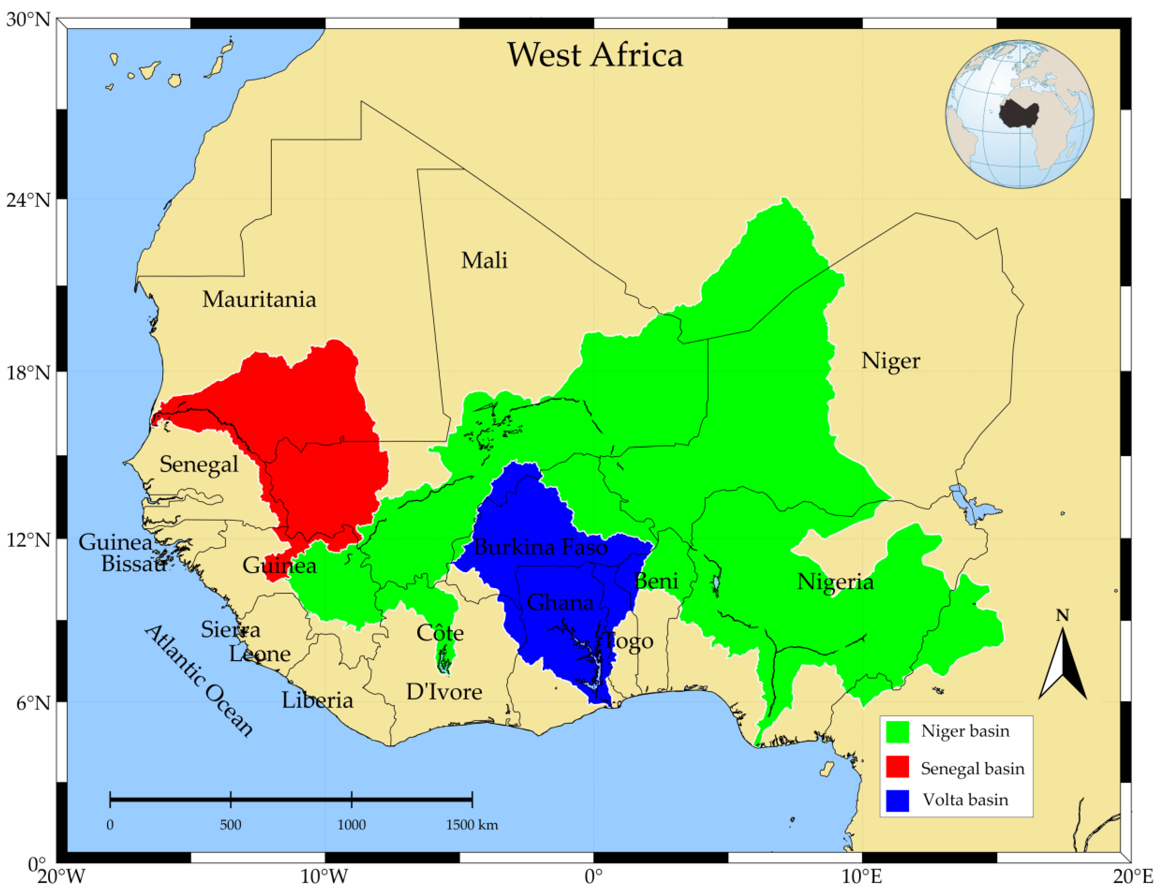
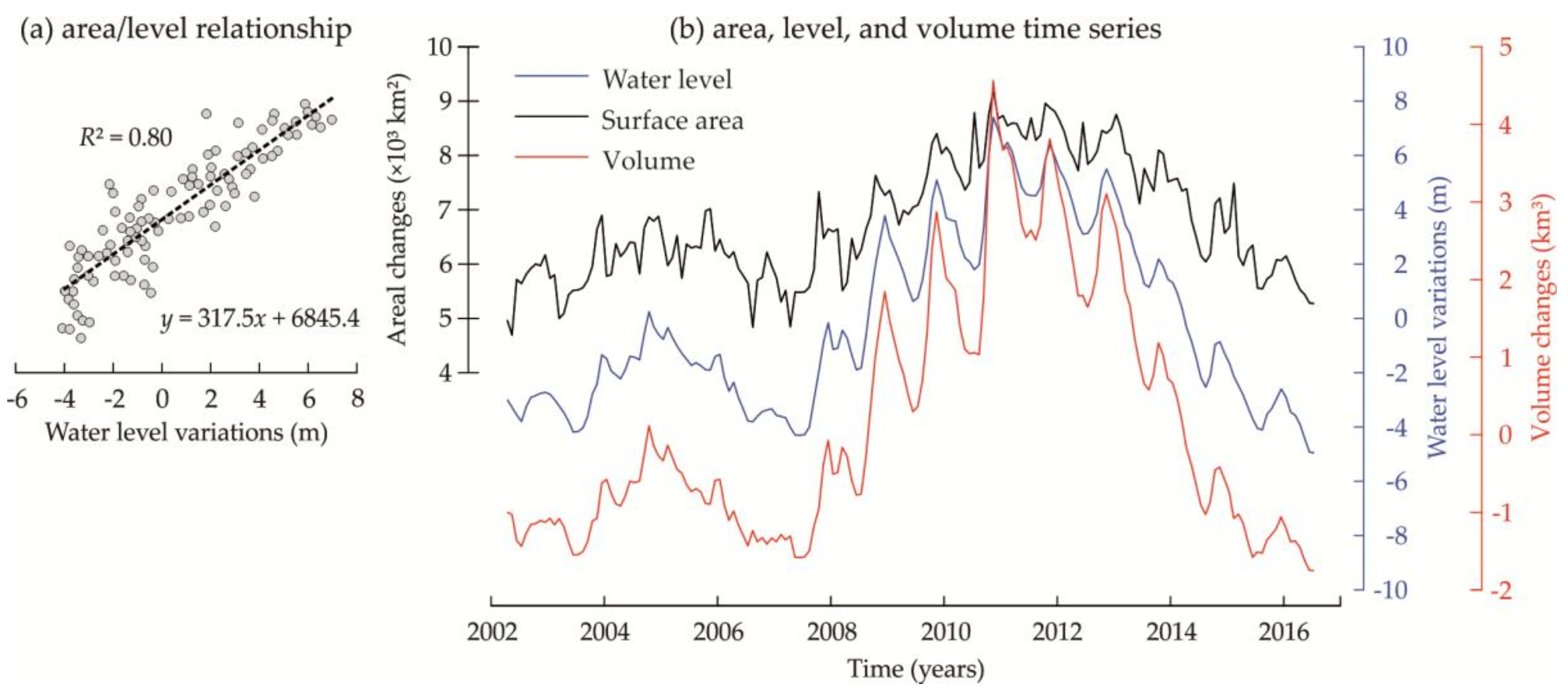
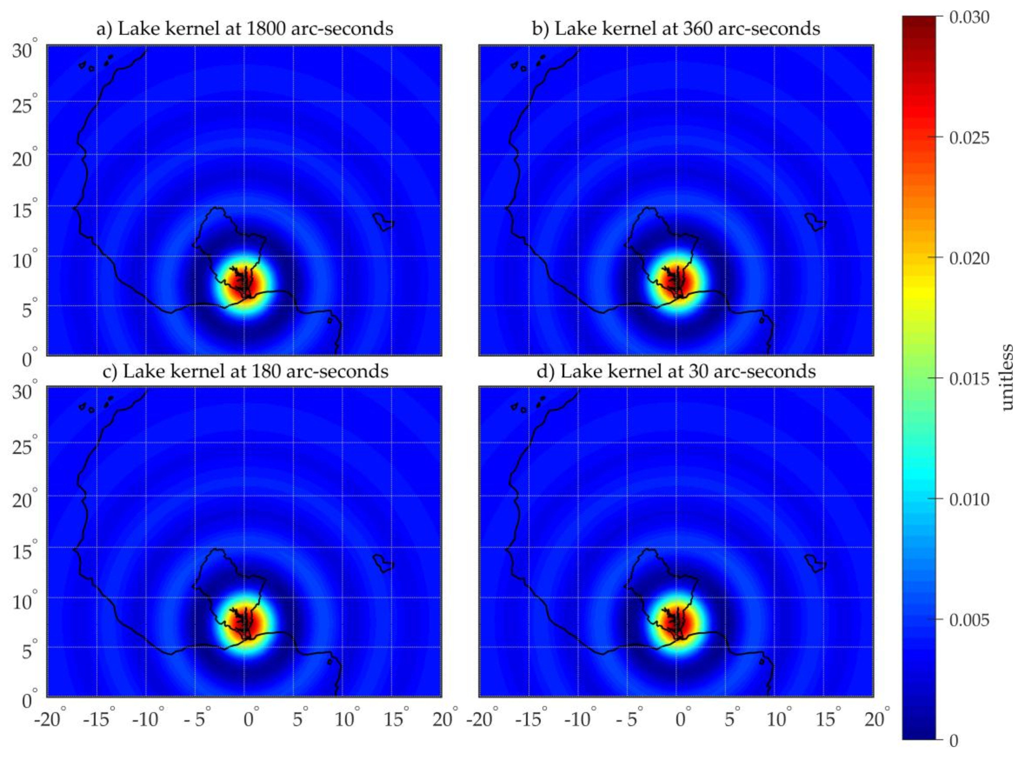
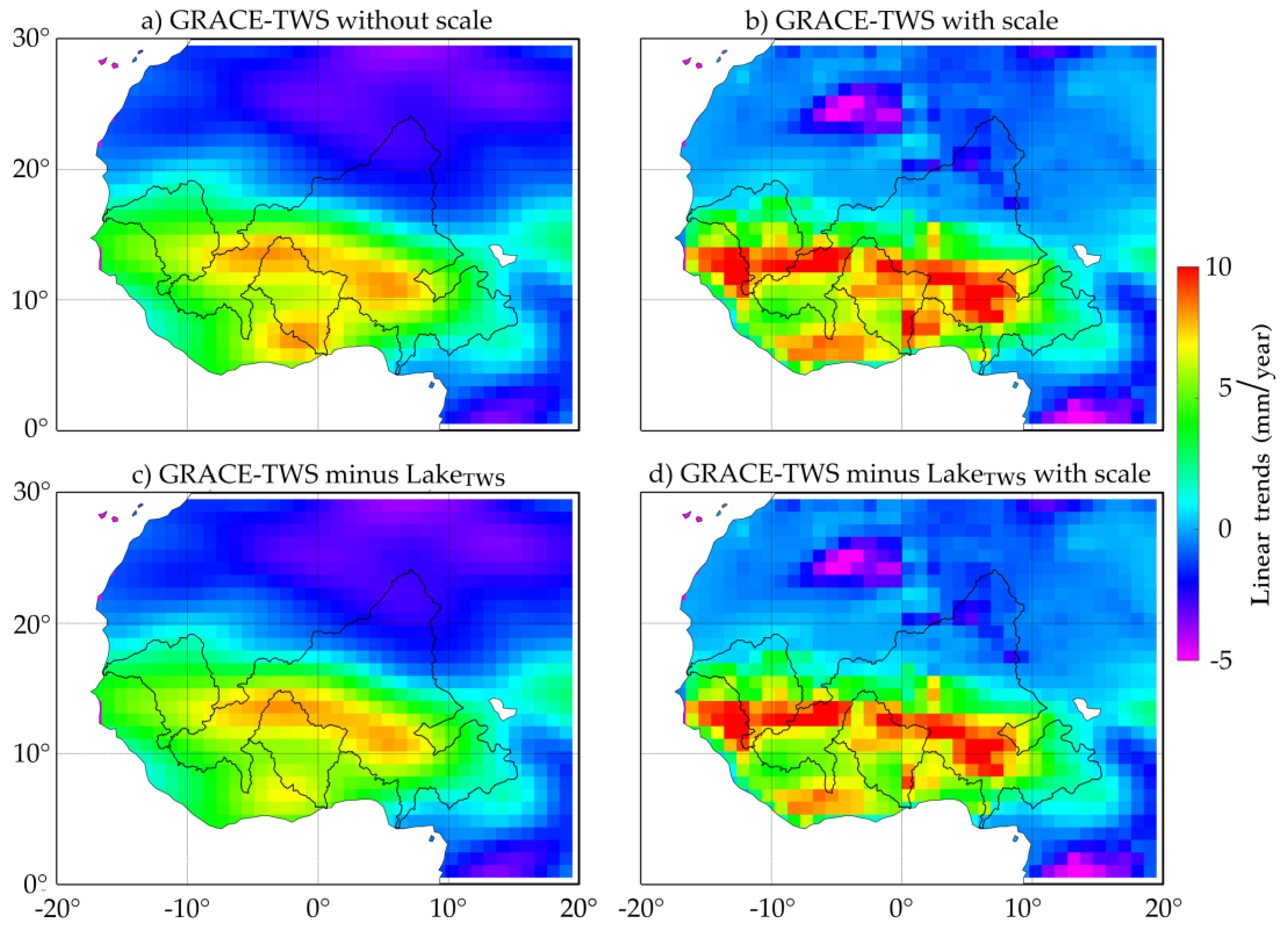
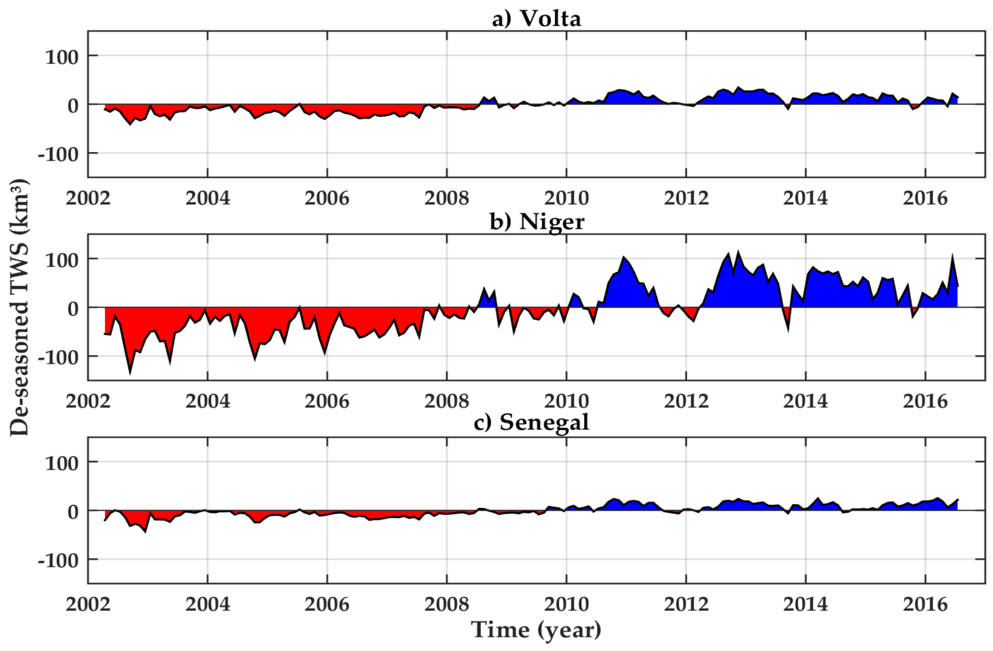
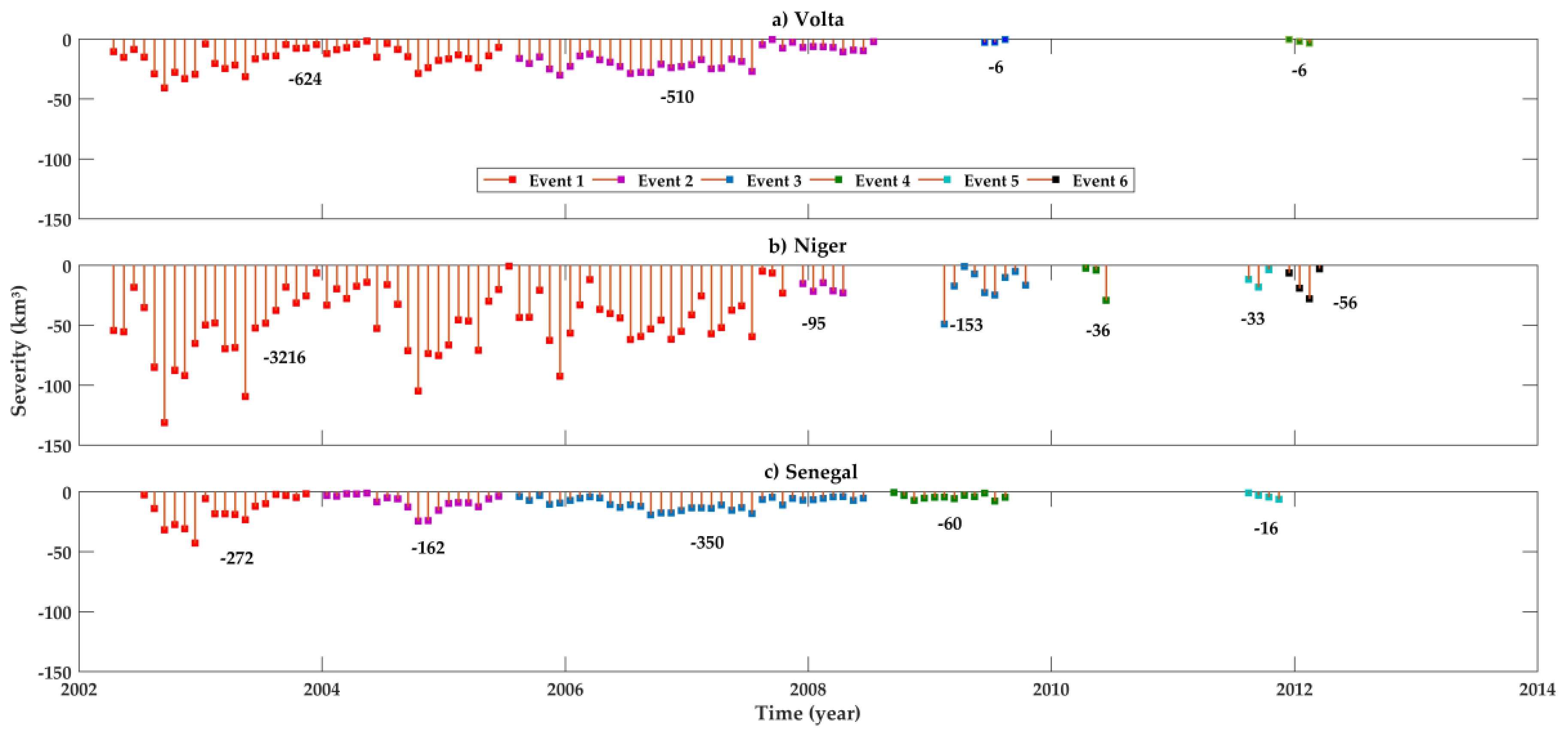
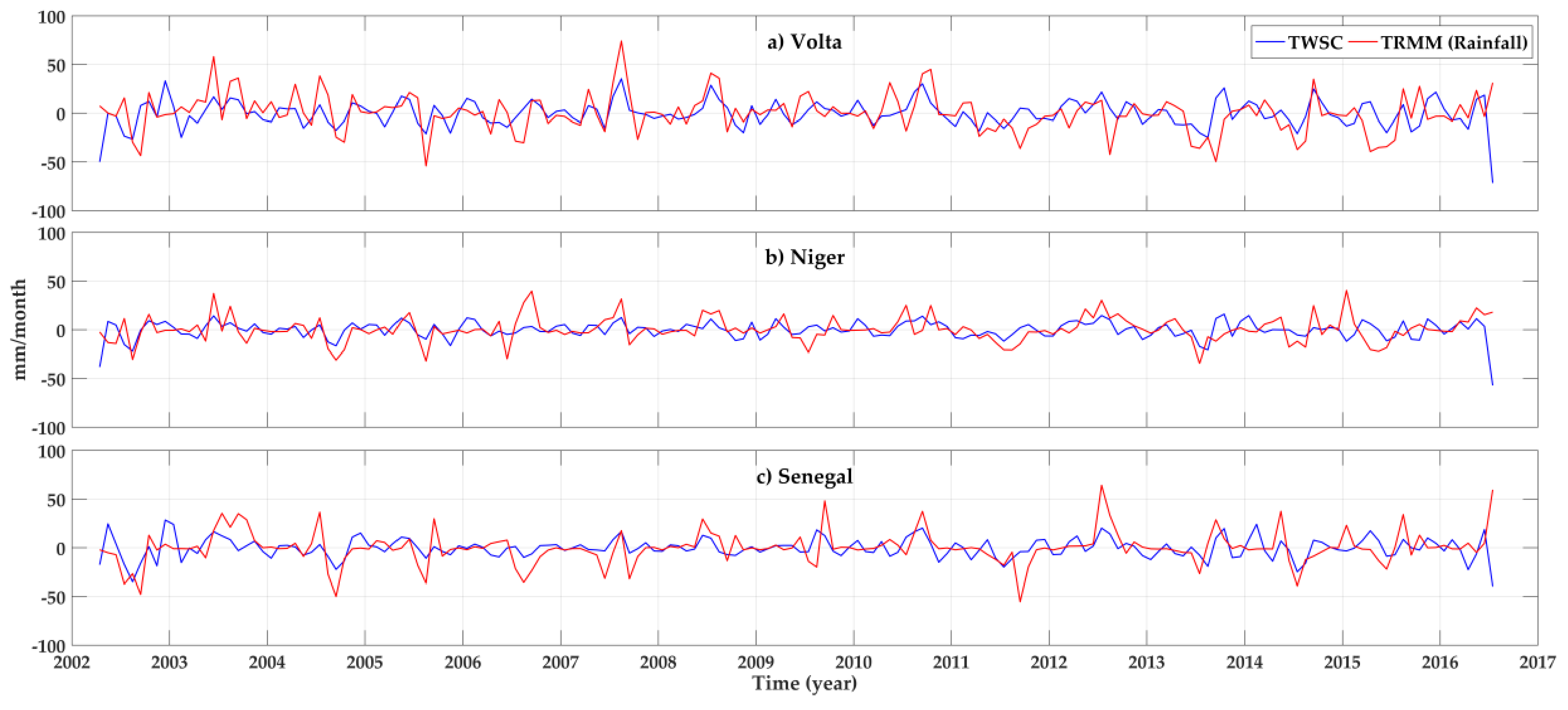
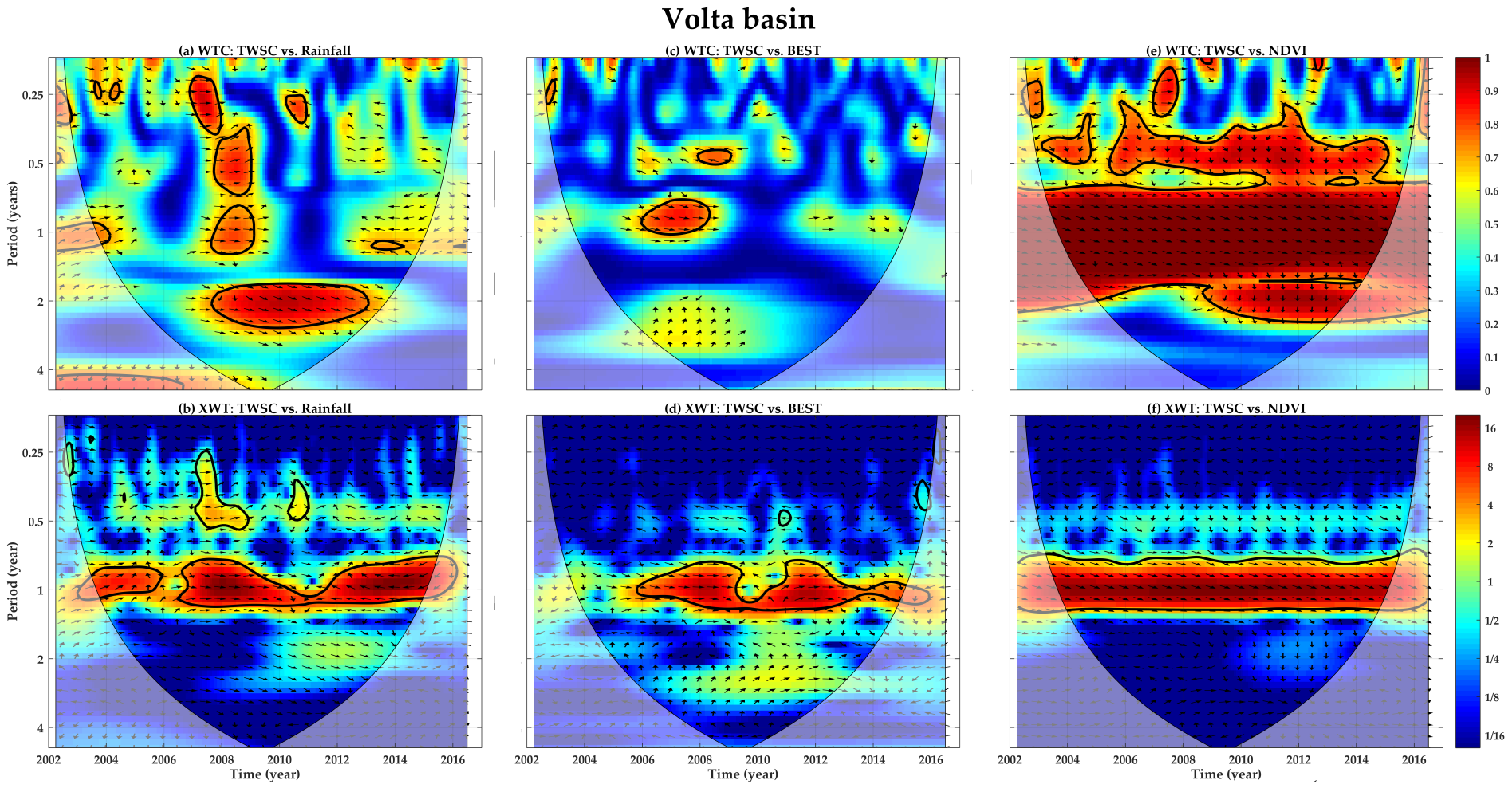
Table 1.
A summary of the GRACE–identified hydrological droughts over the major basins of WA.
| Basin | No. of Events ≥3 Months | Time Frame of Each Event | Duration (Months) | Peak Magnitude (km3) | Average (km3) | Severity (km3/Month) |
|---|---|---|---|---|---|---|
| Volta | 4 | 2002-04 to 2005-05 | 39 | −50 (2002-09) | −16 | −624 |
| 2005-08 to 2008-07 | 36 | −30 (2005-12) | −17 | −510 | ||
| 2009-06 to 2009-08 | 3 | −3 (2009-06) | −2 | −6 | ||
| 2011-12 to 2012-02 | 3 | −4 (2012-02) | −2 | −6 | ||
| Niger | 6 | 2002-04 to 2007-10 | 67 | −131 (2002-09) | −48 | −3216 |
| 2007-12 to 2008-04 | 5 | −23 (2008-04) | −19 | −95 | ||
| 2009-02 to 2009-10 | 9 | −50 (2009-02) | −17 | −153 | ||
| 2010-04 to 2010-06 | 3 | −29 (2010-06) | −12 | −36 | ||
| 2011-08 to 2011-10 | 3 | −18 (2011-09) | −11 | −33 | ||
| 2011-12 to 2012-03 | 4 | −28 (2012-02) | −14 | −56 | ||
| Senegal | 5 | 2002-07 to 2003-11 | 17 | −43 (2002-12) | −16 | −272 |
| 2004-01 to 2005-06 | 18 | −25 (2004-10) | −9 | −162 | ||
| 2005-08 to 2008-06 | 35 | −19 (2006-09) | −10 | −350 | ||
| 2008-09 to 2009-09 | 12 | −8 (2009-07) | 5 | −60 | ||
| 2011-08 to 2011-11 | 4 | −6 (2011-11) | −4 | −16 |
Note: Column (1): basin’s name; Column (2): number of events; Column (3): time span of each event (YYYY-MM format); Column (4): duration; Column (5): peak magnitude, the maximum value of the deficit M that occured during a hydrological drought in km3 at en epoch (YYYY-MM); Column (6): average water storage deficits (km3); Column (7): total severity (S) in km3/month.
© 2018 by the authors. Licensee MDPI, Basel, Switzerland. This article is an open access article distributed under the terms and conditions of the Creative Commons Attribution (CC BY) license (http://creativecommons.org/licenses/by/4.0/).
Share and Cite
MDPI and ACS Style
Ferreira, V.G.; Asiah, Z.; Xu, J.; Gong, Z.; Andam-Akorful, S.A. Land Water-Storage Variability over West Africa: Inferences from Space-Borne Sensors. Water 2018, 10, 380. https://doi.org/10.3390/w10040380
AMA Style
Ferreira VG, Asiah Z, Xu J, Gong Z, Andam-Akorful SA. Land Water-Storage Variability over West Africa: Inferences from Space-Borne Sensors. Water. 2018; 10(4):380. https://doi.org/10.3390/w10040380
Chicago/Turabian StyleFerreira, Vagner G., Zibrila Asiah, Jia Xu, Zheng Gong, and Samuel A. Andam-Akorful. 2018. "Land Water-Storage Variability over West Africa: Inferences from Space-Borne Sensors" Water 10, no. 4: 380. https://doi.org/10.3390/w10040380
Note that from the first issue of 2016, this journal uses article numbers instead of page numbers. See further details here.