1. Introduction
The understanding of complex flow features, as a consequence of complex geometries or hydrodynamic boundary conditions, is very important for the analysis of transport of substances or sediment in rivers and coastal waters, as well as for navigability analysis in waterway projects. The study of those features generally involves sophisticated physical and numerical modeling approaches [
1]. Unfortunately, validation with and scaling to real field conditions are still challenging, due to temporal or spatial constraints of field measurement technologies. Whereas lab or numerical data are available in high frequency and high spatial resolution (e.g., particle image velocimetry (PIV) and laser Doppler anemometry (LDA) [
2], field data are usually measured at fixed points or along transects, and in the past were limited to mean velocity measurements (no turbulence quantities). Also, regarding extraordinary geometries, such as deep and narrow bedrock canyons, the conventional modeling laws are untested and are most probably not applicable.
Nowadays, acoustic technologies are more accessible and improved, presenting considerable advances in the quality of the field measurements. Compared to intrusive and punctual devices (current meter), acoustic instruments, such as the acoustic Doppler current profiler (ADCP), have been used in conventional, hydrological river measurements (discharge, depth, velocity), yielding increased accuracy and greater spatial and temporal resolution due to hardware improvements providing better accuracy for positioning, but also having several frequencies combined in the same devices, as well as being robust equipment for field deployment, especially compared to optical (e.g., LSPIV) techniques [
3]. Recently, higher spatial resolutions were obtained by mapping individual ADCP velocity profiles over large flow areas, as presented by Flener et al. [
4] or Jamieson et al. [
5], where the latter included measured sections with 5 and 20 m spacing upstream and downstream of two different wing dikes for three different discharges.
Using the Doppler effect of acoustic waves scattered back from particles within the water column, ADCP is proven to measure velocity, depth, and water discharge accurately with high resolution (cm) [
6]. Besides the depth and the mean velocity components, additional data inherent to the acoustic measuring method can be analyzed, such as the backscatter intensity and velocity standard deviation. For example, ADCP data have been used to derive other flow characteristics, such as mixing coefficients [
7,
8,
9], sediment transport rates [
5], and moving bed velocity [
10]. The flow velocity information has also been used for profile analysis and mapping of integrated or characteristic quantities, such as bed shear stress and depth-averaged velocity [
6,
11]. Moreover, acoustic backscatter signal and its statistics can be used for a suspended sediment transport analysis [
12]. The velocity standard deviation information (velocity’s second-moment statistics), can be explored to obtain turbulence quantities [
13,
14], which will be the focus of this article. This parameter is especially of interest when analyzing and modeling complex flow situations, where strong and large secondary currents exist (3D effects), creating non-conventional turbulence distributions (non-logarithm velocity profiles), thus limiting resistance law-based approaches or hydrostatic modeling concepts.
Bedrock Rivers can present morphology variations of width and depth over small distances caused by climatic variations, abrasion, cavitation or tectonic movements. Relatively narrow and deep canyons emerge in locations of active bedrock incision, sometimes in association with tectonic fault lines [
15]. Narrow canyons have flow characteristics (hydraulic radius, velocities, and turbulent effects) vastly different from less confined reaches, with the presence of vertical accelerations and secondary currents that influence the shape of the velocity profiles. Analyzing the flow in canyons of the Fraser River (Canada), Venditti et al. [
16] described the flow as nonlinear and with strong secondary circulation and high levels of turbulence. At the entrance to canyon pools, they observed a plunging core of high velocity flow, which suppressed the maximum velocity below the free surface.
The objective of this paper is to obtain turbulence and secondary current information for flow analysis and model calibration in complex flow environments in a peculiar and morphologically unique submerged bedrock canyon of the Tocantins River in Brazil, a tributary of the Amazon estuary. As the canyon reach is considered an obstruction point for navigation within the important Tocantins waterway, recent studies were undertaken to evaluate and plan river engineering projects for Brazil’s National Transport Infrastructure Department (DNIT).
The spatial distributions of bed shear stress (τ0) and eddy viscosity (υt) were assessed in this river reach, based on extensive ADCP measurements collected from a moving boat to better understand the river dynamics in this submerged bedrock canyon. Using this real field-scale case study, three different approaches were used to calculate bed shear stress: the total kinetic energy (TKE) method, law of the wall method and the depth–slope product method. With the results of the TKE method, the eddy viscosity was estimated with the Boussinesq approach.
2. Materials and Methods
2.1. Bedrock Canyon of Tocantins River
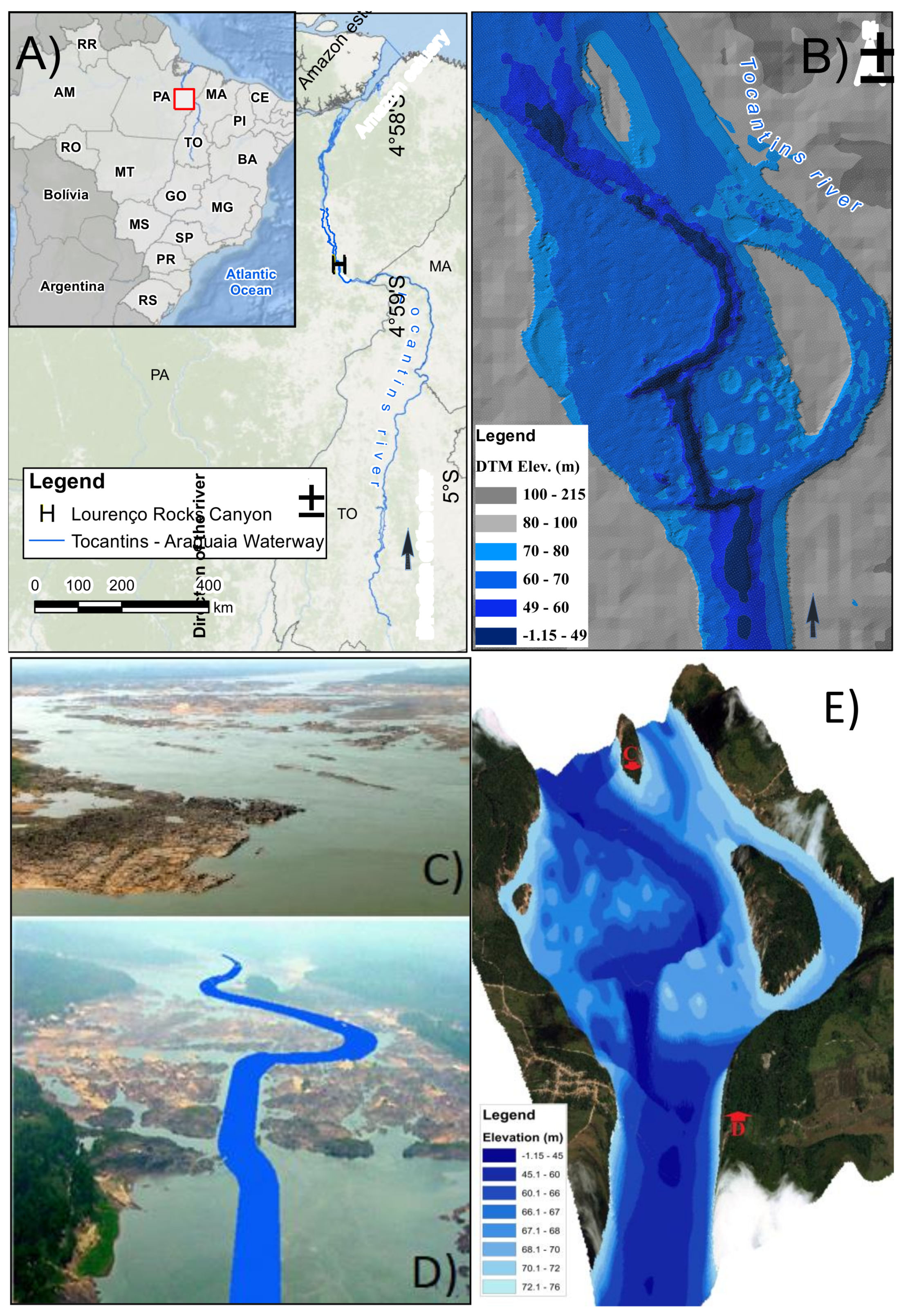
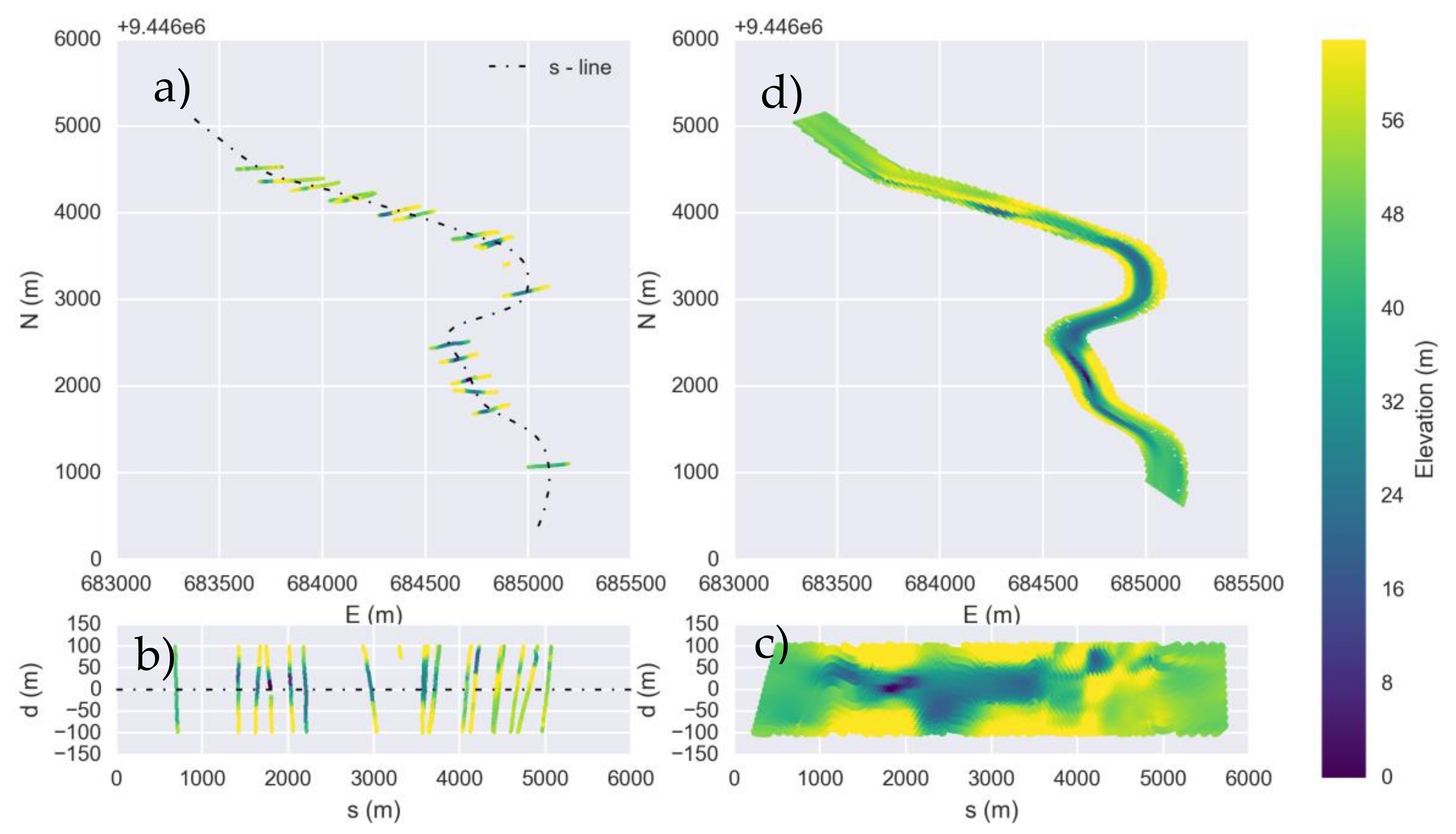
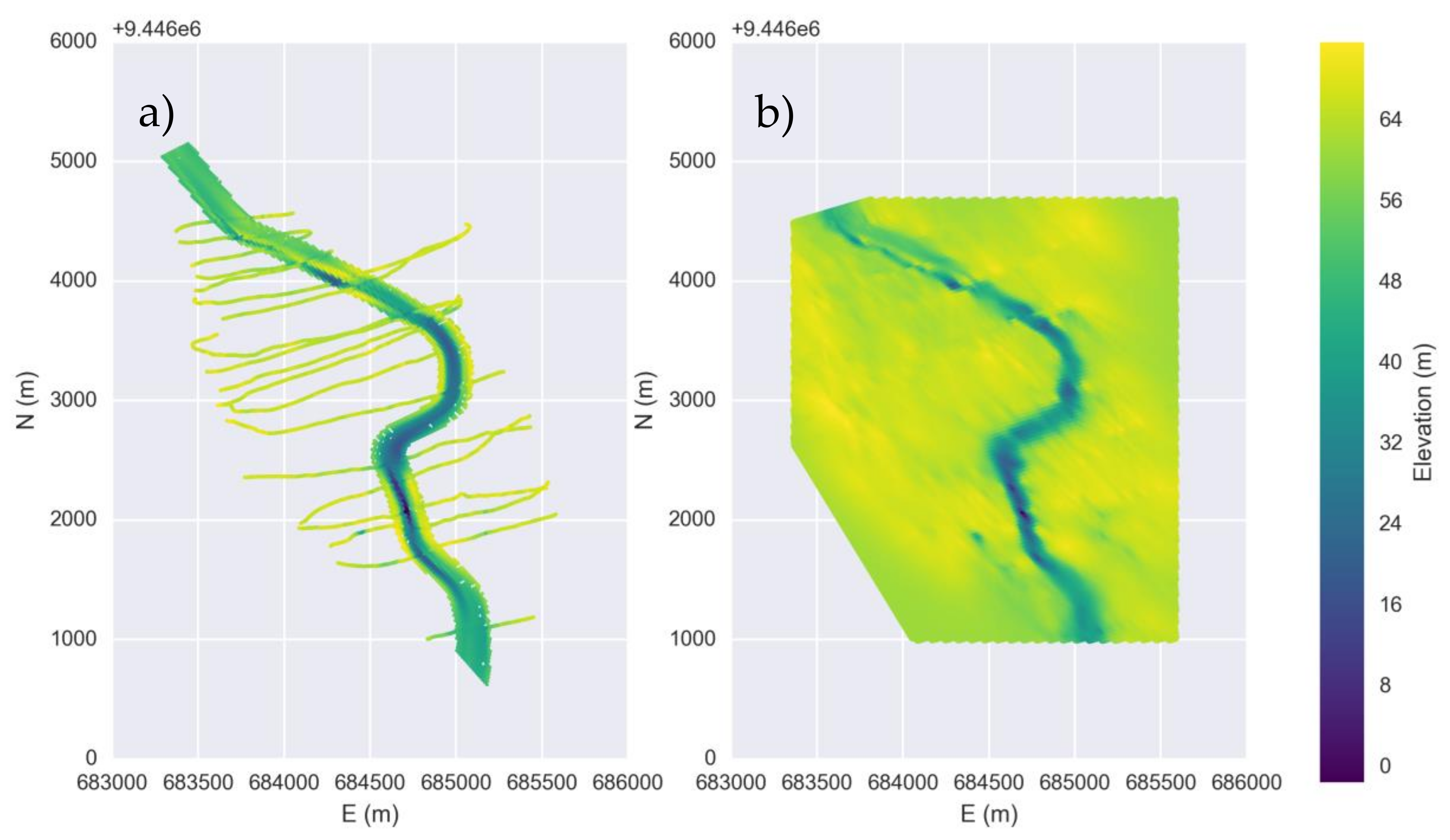
The study area is named Lourenço’s Rock Canyon (
Figure 1), a reach of Tocantins River, one of the largest and most important rivers in Brazil. Located in northern Brazil, the Tocantins River is the main river of the Tocantins-Araguaia Basin, the second largest hydrographic basin in the country with 967,059 km
2, smaller only than the Amazon River Basin.
The Tocantins-Araguaia waterway is one of the main transportation routes of Brazilian products for export, such as minerals and agricultural commodities. Nowadays, the Lourenço Rock Canyon is considered one of the most significant obstructions to navigation in the Tocantins River. Despite the high depth, the canyon path presents a sharp curve and the available width is not adequate for safe navigation during the drought season and for the commonly used vessels. Moreover, through the flood season, the canyon induces strong shear flows, making navigation more difficult and less safe. According to DNIT [
17,
18], the Brazilian Government is investing more than U
$150 million in engineering projects to improve the navigation channel in the study area.
The submerged bedrock canyon is 6 km long, and its depth can reach 60 m (upstream and downstream of the canyon reach the river has a depth of 7 m). The annual mean flow in the reach is 11,800 m3/s, with high seasonal variations ranging from 1898 to 45,717 m3/s. During the flood season, the river width is around 1.5 km, with the presence of a few rocky outcrops, high velocities and strong turbulent flow (large shear layers and longitudinal vortices). During the drought season, the flow is confined along the canyon area (150 m width), exposing the river bedrock at the reach. Although having smaller diameters, the presence of vortices is constant, even under low flow conditions.
According to the Brazilian Mineral Resources Research Company [
19], the river reach is located between two tectonic domains, the Couto Magalhães Formation (part of the Tucuruí Group) and the Bacajá Domain (part of the Transamazonas Province). The river bed is composed of sandstone Rock from the Itapecuru (K12it), Pastos Bons (J2pb) and Grájau (K1g) formations on the undifferentiated fractured basement (Fr). The canyon’s origins can be associated with the Tucuruí Fault, caused by tectonic movements that generated a series of structural features in the lithologies and later migmatites, which also induced a dynamic metamorphic event in the rocks under green-schist facies conditions.
2.2. Equipment and Field Data
In April (flood season) and October (drought season) 2015, several flows and velocity measurements were performed in Lourenço’s Rock Canyon using an acoustic Doppler current profiler (ADCP), model M9, series SN-3754 of Sontek Inc. (San Diego, CA, USA) [
20]. The equipment was installed with fixed support on a moving boat, and the installation depth of the transducer was 0.47 m below the water surface. The equipment was coupled to a real-time kinematic (RTK) global positioning system providing sub-decimeter accuracy for the measurement coordinates.
As the boat traverses the sampling area, each vertical depth profile (ensemble) is subdivided into several cells (bins), and the velocity profile for each compass axis (easting, northing, and vertical) is calculated for each of the four inclined beams. An internal compass and tilt sensor provide compensation for boat movements. As only three beams are necessary to compute the three velocity components, additional information can be obtained when using ADCPs with four transducers (similar to the one used here), where the fourth beam provides a redundant measurement of vertical velocity, from which velocity heterogeneities and turbulence variations may be quantified. The ADCP can be operated in 3 different modes: NarrowBand, Pulse to Pulse and Broadband [
21]. In NarrowBand mode, the transducers emit, in a short period (e.g., 1 s), several pulses (pings) and the water velocity is calculated based on statistical analysis of the received signals. As a result, for every ensemble profile measurement, a short time series is produced along each axis in each depth cell, with a mean velocity (<u>, <v>, <w>) and a standard deviation (σ
x, σ
y, σ
z). Some ADCP brands supply all the velocity samples from the time series, allowing the user to calculate the statistics; however, the M9 only provides the results of mean velocity and standard deviation, which will be used here.
The ADCP M9 is a double frequency instrument, with four transducers (25° from vertical) at both 1 MHz and 3 MHz. The frequency and thus cell sizes are changed automatically on-the-fly depending on the local water depth, if not configured otherwise. Along the sections in the Lourenço’s Rock Canyon, the shallow margins were usually measured with a frequency of 3 MHz, and the deeper canyon with 1 MHz, both in Narrowband mode. The vertical dimension of the measurement cells (ΔZcel) varied between 0.1–0.5 m for the 3 MHz and 0.5–2.0 m for the 1 MHz. The horizontal sampling dimension is determined as a function of the boat’s movement in time, and the data acquisition frequency (f = 1 s). Also, there is a vertical beam of 0.5 MHz in the middle of the instrument head to improve bed level measurements. The Sontek M9 maximum depth for velocity measurements is 40 m, and some parts of the canyon were more than 50 m deep, thus resulting in larger blanking areas near the bottom. Nonetheless, the bed level was measured throughout the canyon using the vertical beam.
Although measurements are available for both flood and drought season, only the data of the flood situation have been processed so far regarding the methods presented in this manuscript. Thus, all following results are based on the flood situation only, being the more interesting one in terms of the observable features and processes.
The mean discharge during the April 2015 flood flow situation was 18,275 m
3/s. Several transversal sections and a longitudinal zig-zag type of measurement were undertaken along Lourenço’s Rock Canyon during a short period (short enough to have discharge changes of less than 3%). The measurement resulted in 10,531 velocity profiles (ADCP ensembles) at different points of the canyon, each having on average about 14 cells, thus resulting in approximately 140,000 3D velocity vectors.
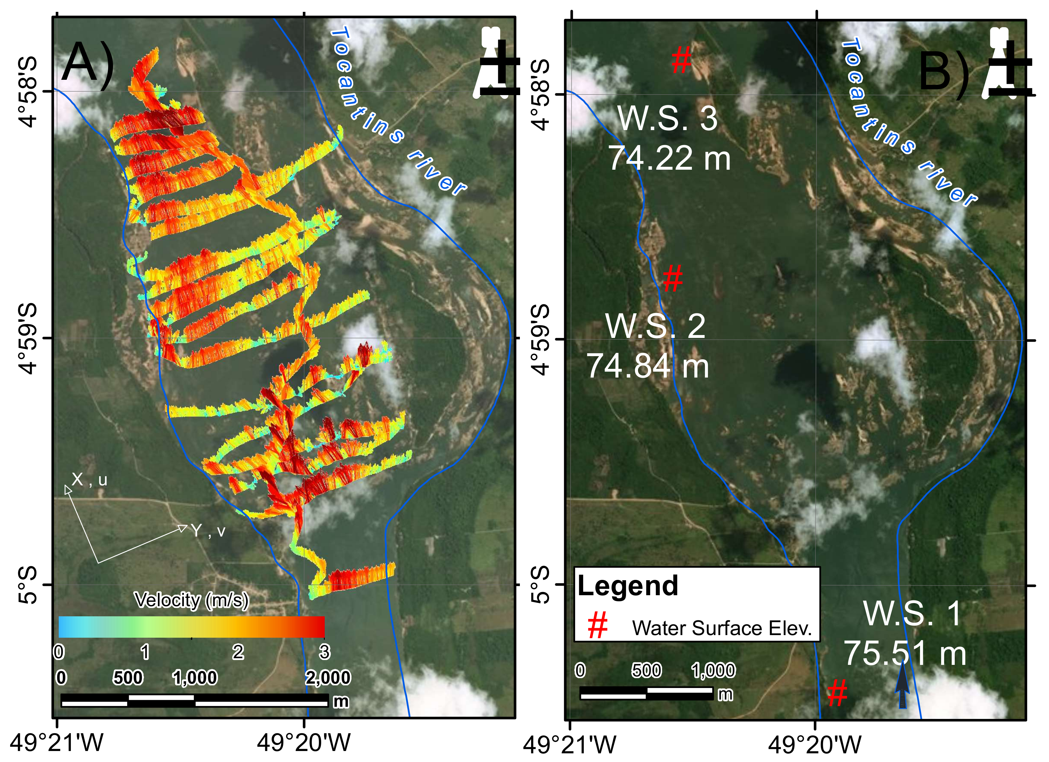
Figure 2 shows the location of the spatial measurements. Three Elevation Reference (ER) stations were installed and geo-referenced along the study area using the Global Navigation Satellite System (GNSS). The ADCP’s compass was calibrated three times during the measurement. The water surface elevation measured at each point is presented in
Figure 2, and the resulting mean water surface slope (S
WS) was 2.36 × 10
−4 m/km. A detailed bathymetry measurement of the area was available from previous measurements in 2012, with both single and multi-beam echosounder equipment. A DTM (Digital Terrain Model) was created (
Figure 1), combining the bathymetry data with SRTM (Shuttle Radar Topographic Mission) data to complete the margin information.
2.3. Initial ADCP Data Processing
The equipment’s software Riversurveyor [
20] was used to export all the velocity profiles into Matlab [
22] file formats. The data coordinate system was ENU (East-North-Up), the depth reference used was the vertical beam (VB) and the boat velocity used as reference the bottom track (BT) feature. Subsequent post-processing was done using a recently programmed toolbox, VelMap [
23]. The toolbox can decompose the velocity data measurements by rotation as a function of an angle chosen by the user. For the study area, an angle equal to 337° clockwise from North (angle = 0°), was considered the longitudinal flow direction (x-axis), and 247° as the transversal (y-axis. This fixed coordinate system has been chosen here due to the large heterogeneities in the flow and thus difficulties in defining a consistent main flow direction. The chosen angle, however, corresponds to the overall mean velocity direction. Moreover, the toolbox uses additional parameters (SNR—signal to noise ratio, STD—standard deviation) for further processing, following instrument specifications.
Many factors affect the uncertainty of ADCP measurements, such as instrument noise and configuration, velocity fluctuations due to flow turbulence, bottom track errors, compass errors and GPS errors [
6]. According to Sontek [
24], the standard deviation of the velocity data can be attributed to installation and calibration problems, acoustic noise from the equipment, and velocity fluctuations from the local turbulence. Following [
25,
26], installation and calibration errors were considered negligible, and the standard deviation for each velocity component decomposed as:
where σ is the standard deviation from the velocity data (m/s); σ
t is the velocity fluctuation from the local turbulence (m/s); σ
n is the acoustic noise effect from the equipment on the standard deviation (m/s). The acoustic noise is a result of the physical process by which sound waves are dispersed by the solid particles in the water. To estimate the turbulent part of the standard deviation, previous approaches calculated the acoustic noise using different assumptions. Vachtman and Laronne [
27] considered the acoustic noise equal to the minimum variance of calculated water velocities for all depth cells (σ
n2 = σ
2min). Another approach was presented by Rennie and Church [
6], who applied Equation (1), but used the average ADCP error velocity (σ
error), instead of the acoustic noise. The average ADCP error velocity considered other uncertainties and can be calculated by the velocity difference (V
d) from 2 vertical velocity measurements and the horizontal velocity error (V
e). According to Sontek [
24], although being a random effect, it can be assumed that acoustic noise follows a Gaussian distribution. The magnitude of the noise can vary according to the equipment frequency (F), the vertical dimension of the cell (ΔZ
cel) and the number of pings (N) emitted in the period measured per cell. For a standard 3D ADCP measurement, the acoustic noise can be estimated with Equation (2).
Developed by the same manufacturer, Equation (2) was defined for older ADCP models than the M9. Conferring with Sontek [
28], there is not yet a specific noise equation for the M9. It is herein assumed that the results from Equation (2) can be used as the best approximation of the noise from the ADCP data.
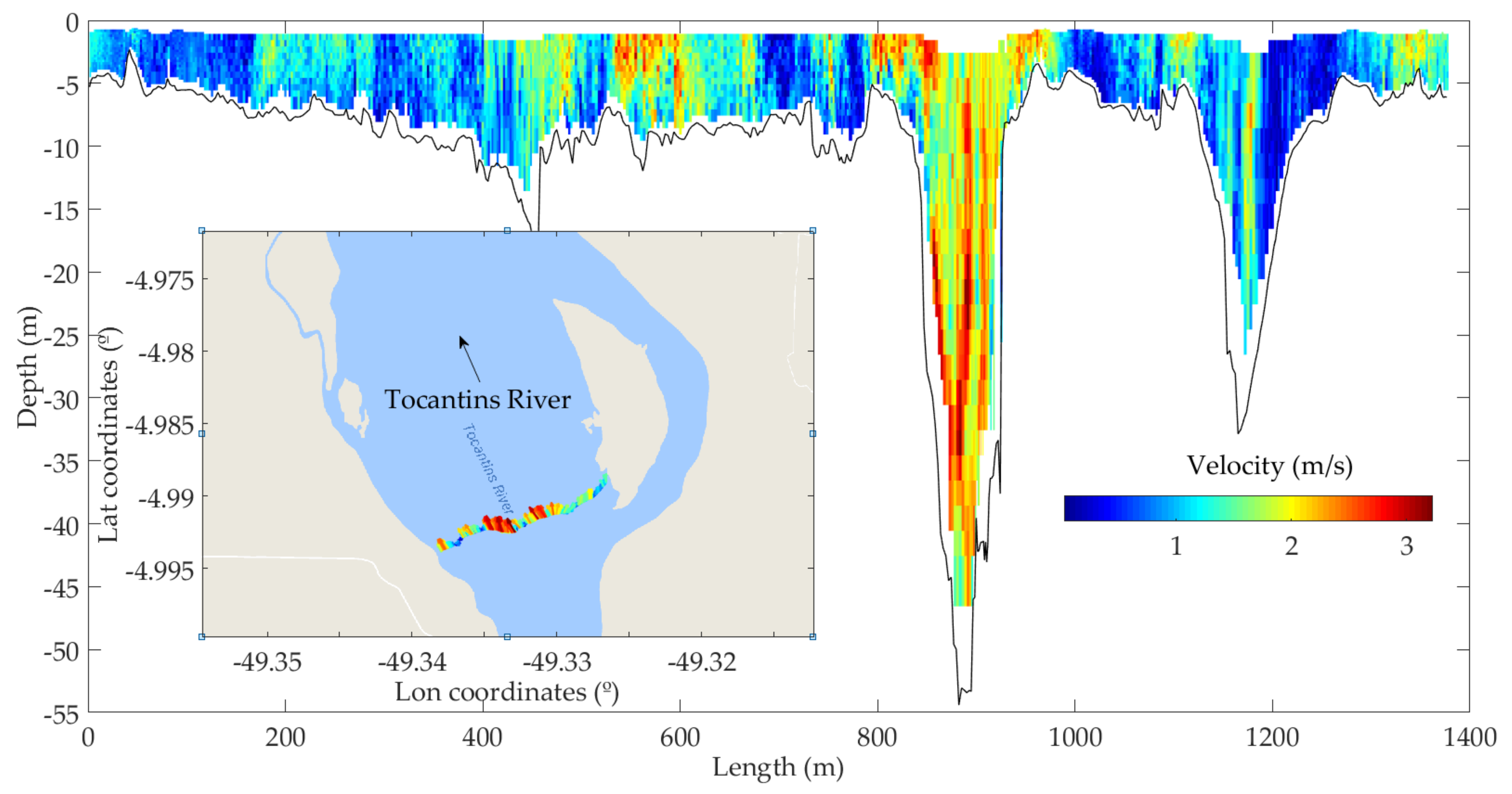
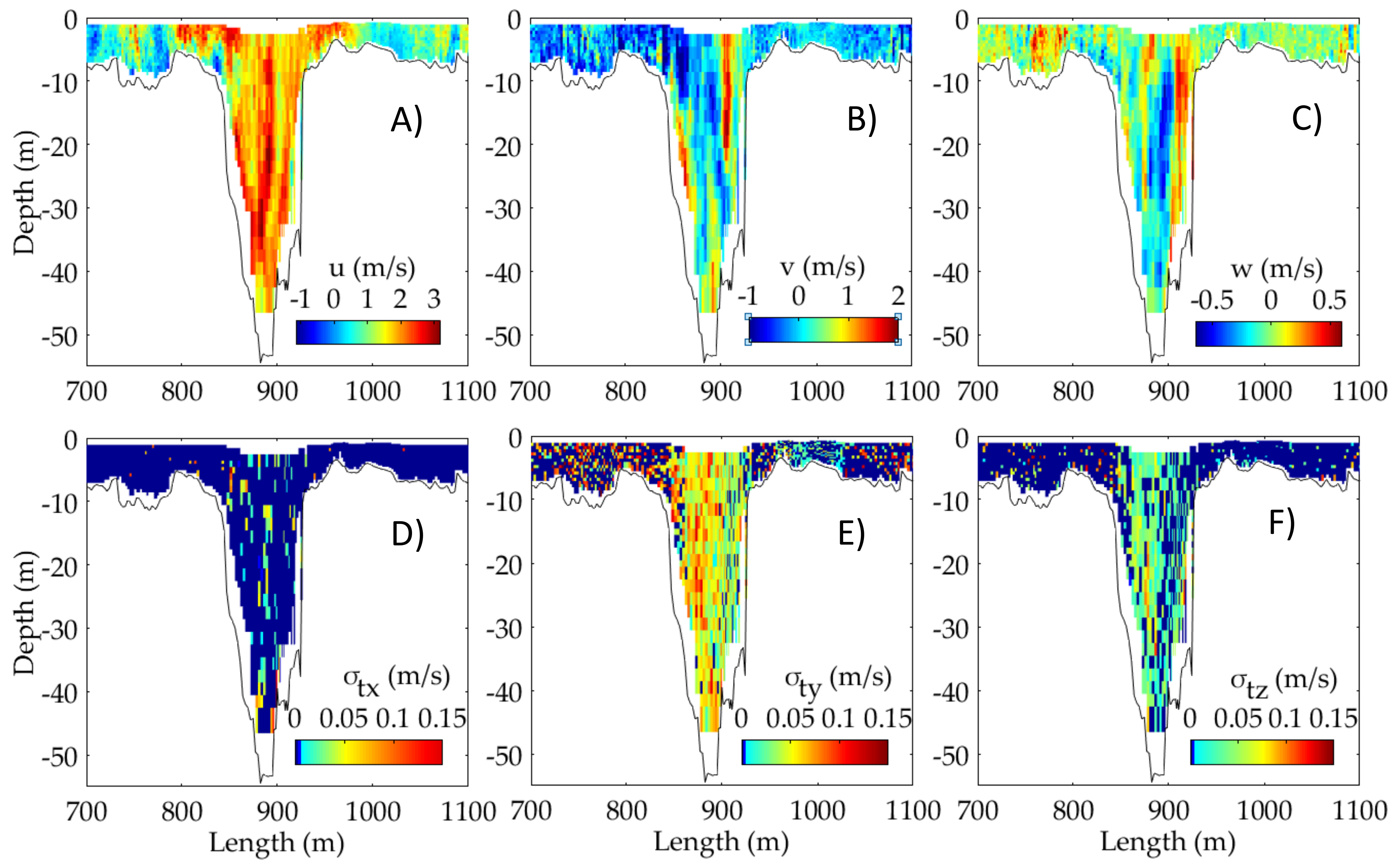
All results can be visualized as velocity magnitudes along a cross-section for each mean velocity component (<u>, <v>, <w>), related velocity fluctuations from the local turbulence (σ
tx, σ
ty, σ
tz) and computed flow parameters (turbulent kinetic energy k and shear stress τ), as shown in Figures 5–7, and explained in the following section. The velocity distributions show the part of the canyon with highest velocities and highest longitudinal velocities occurring in the deeper part of the channel. These effects follow the observations by Venditti et al. [
16], where similar flow features were observed for a bedrock canyon of the Fraser River.
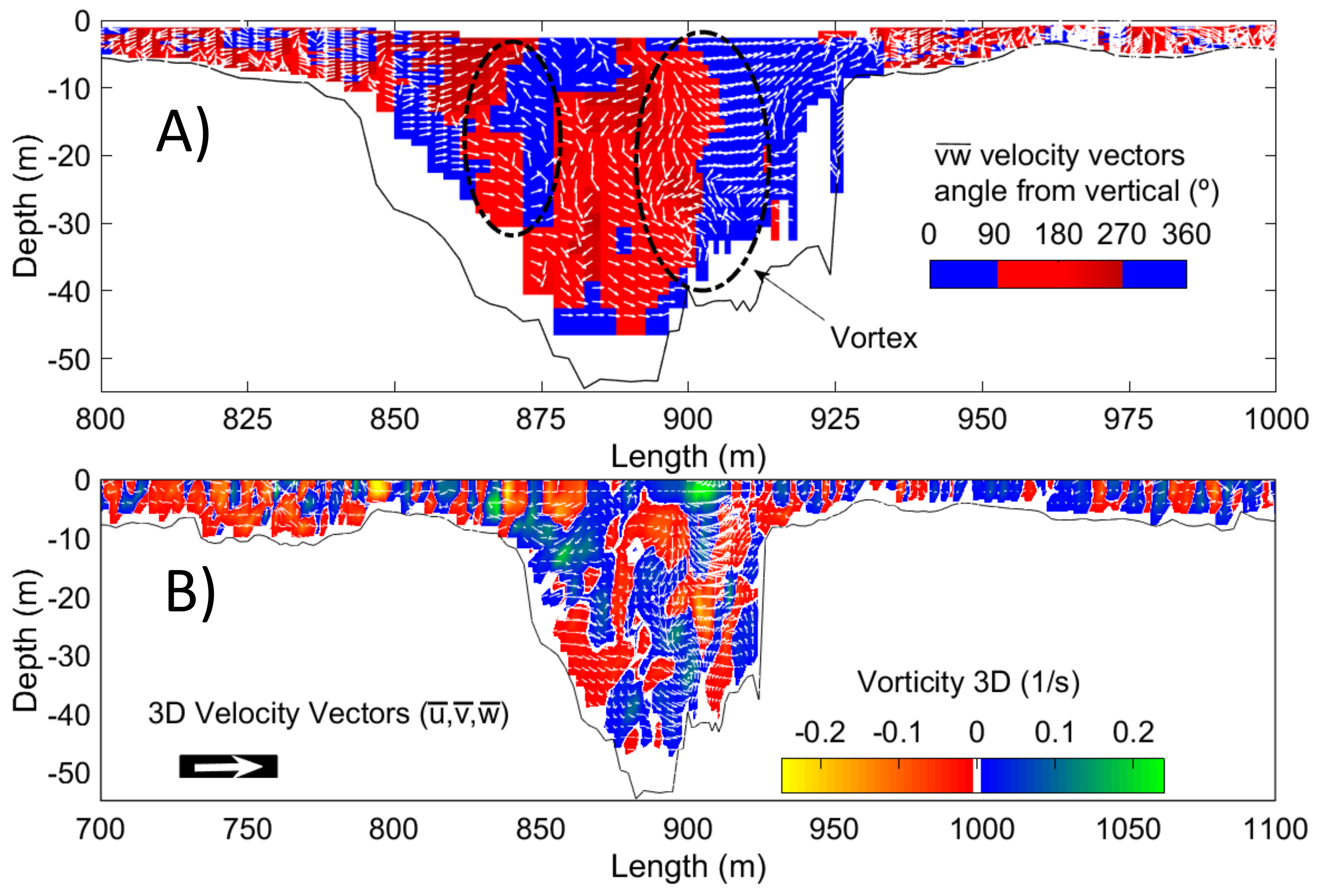
The strongest transversal velocity fluctuations occur in the canyon section. The variations of transversal and vertical velocity components indicate large and strong secondary currents induced by the canyon walls. The secondary currents in the horizontal plane were even visible as strong (boat was shaking), and large (several meters) surface vortices (
Figure 3) also manifested as strong transversal velocity fluctuations. Normally, these large vortices are difficult to observe in natural rivers. However, these vortices can frequently be viewed along the canyon section during the flood season, reinforcing the river reach peculiarity.
3. Theory and Analytical Methods
This section briefly reviews the different methods applied to calculate the local bed shear stress and eddy viscosity distributions, including discussion of details and assumptions.
ADCPs operated from moving vessels have been used in previous studies to estimate spatial flow characteristics. Flener et al. [
4], Rennie and Church [
6], Rennie and Millar [
10], Sime et al. [
11], Szupianyet et al. [
29], Guerrero and Lamberti [
30], are reference studies that mapped some flow characteristics, such as shear velocity, shear stress, suspended and bedload sediment transport. However, in some river structures, such as meanders, bifurcations and submerged canyons, these characteristics are more difficult to estimate because of the high turbulence levels and the nonlinear velocity profiles along the river area [
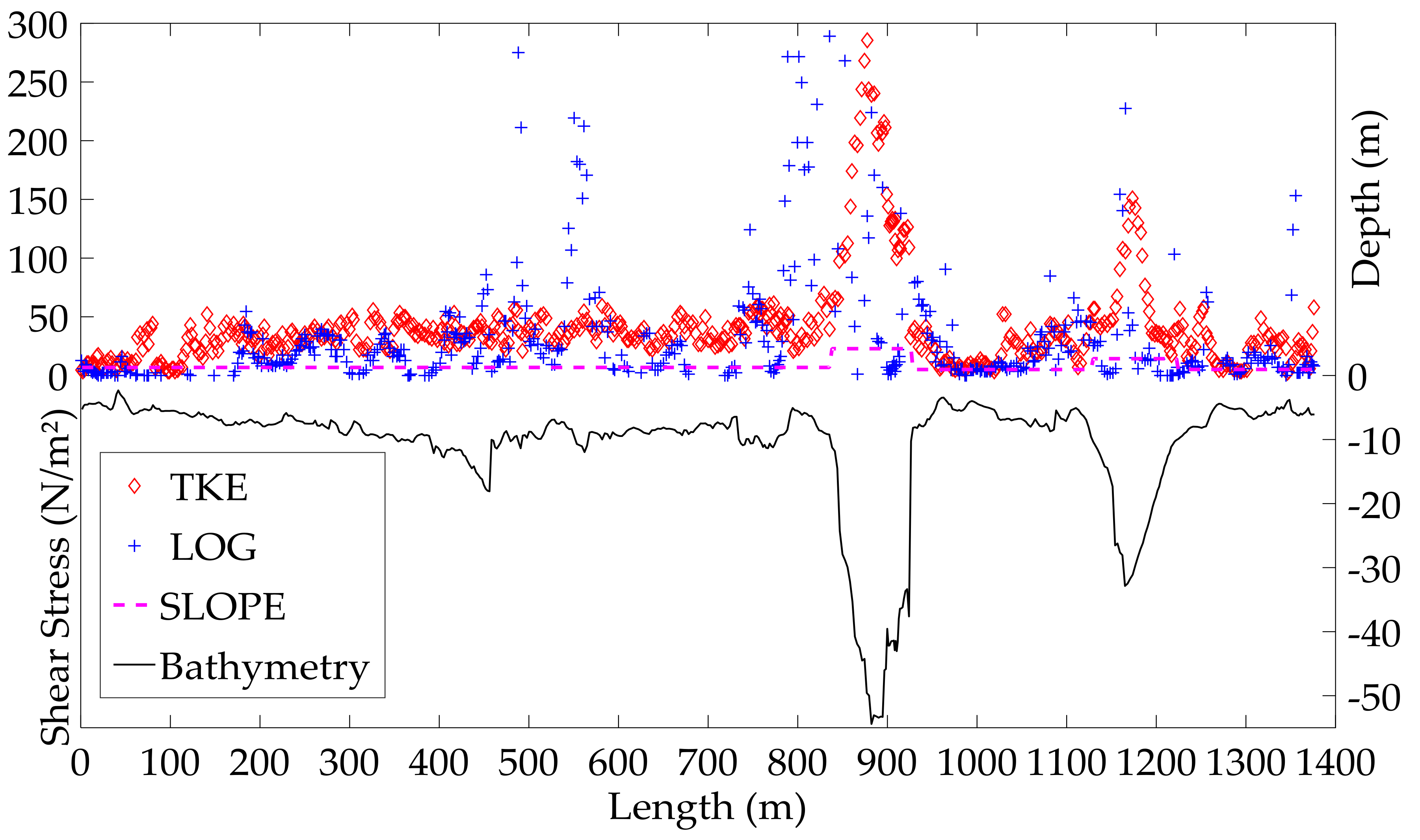
31]. Three different methods to calculate the bed shear stress were compared here to evaluate the flow characteristic of the measured reach.
3.1. TKE Method
All the velocities can be split into mean components (<u>, <v>, <w>) and fluctuating components (u’, v’, w’) using Reynolds decomposition, where the parentheses denote the time-averaged value, and the prime symbol the turbulent fluctuations. Results of the TKE method relate the intensity of velocity fluctuations (u’, v’, w’) to turbulent kinetic energy (k), as described in Equation (4). Based on the hypothesis that the Reynolds stress and the variances in the region near the bottom are practically constant and proportional to the shear velocity (u*), this method has been applied to ADCP data in studies by Lu and Lueck [
21], Nystrom et al. [
32], Hurther and Lemmin [
33], Vachtman and Laronne [
27], Liu and Wu [
34]. Therefore, the shear stress was calculated as:
where C
0 is a dimensionless constant (i.e., C
0 = 0.18–0.21) [
13]; ρ is the water density (i.e., ρ = 1 g/cm
3 at 15 °C). Using the ADCP in Narrowband mode, it is possible to combine the Standard Deviation (STD, Equation (1)) from the velocity data (for each component), and the Reynolds Decomposition to determine the temporal root mean square of the velocity fluctuations (<u’
2>).
By rewriting Equation (4) with the other equations and directions, the shear stress for each cell (τ
0-TKEcel) can be calculated using the velocity STD components of the ADCP data.
The bed shear stress (τ
0-TKE), calculated by the TKE method, can be determined by the integration of the shear stress calculated in each cell (τ
0-TKEcel) of the vertical measurement (ensemble). For the vertical average the variance sum law was applied, where the covariance of the velocity time series between each cell should be calculated; however without the samples, this study considered that the sum of the covariance among the ensemble is equal to zero. Togneri et al. [
35] used the same consideration to compare the ADCP observations with a 3D model simulation. Besides, Lu and Lueck [
21] calculated the distribution (histogram) of the covariance in velocity profiles from an ADCP fixed to the bottom of a tidal channel at a depth of 30 m, during 20-min intervals in 2 different flow events. The results showed a balance between positive and negative covariance, with a mean near to zero.
The numbers of samples in each cell measurement is another relevant point. Depending on the size and duration of the turbulent features to be measured, longer averaging times are required, requiring either anchored boat measurements [
11] or slow boat movements. In the present study, the slow boat moving method with large spatial distribution was chosen to capture large-scale turbulent variations.
3.2. Law of the Wall Method
The log law is often used to estimate shear stress in open channels and rivers, as presented in Keulegan [
36]. Based on the assumption that the velocity profile in open channel flows has a logarithmic shape, the “Law of the Wall” can be described by the von Karman–Prandtl Equation.
where κ is the von Karman constant (i.e., κ = 0.40); U is the velocity at height z above the bed; u* is the shear velocity, and z
0 is the roughness length. For natural rivers, considered as a hydraulically rough flow, Equation (7) can be described using the characteristic roughness length-scale (k
s).
The shear velocity and the roughness length-scale can be estimated using the velocity profile measurement by the ADCP and fitting the data to the following equation.
where m = (u*/κ); b = (u*/κ) ln(30/k
s) = m ln(30/k
s).
The relationship between shear velocity and bed shear stress (τ
0-log), by the log-law, is given by:
According to Pope et al. [
37], this method is only valid for steady, uniform, one-dimensional flow and its application to natural streams does have some limitations. Afzalimehr and Rennie [
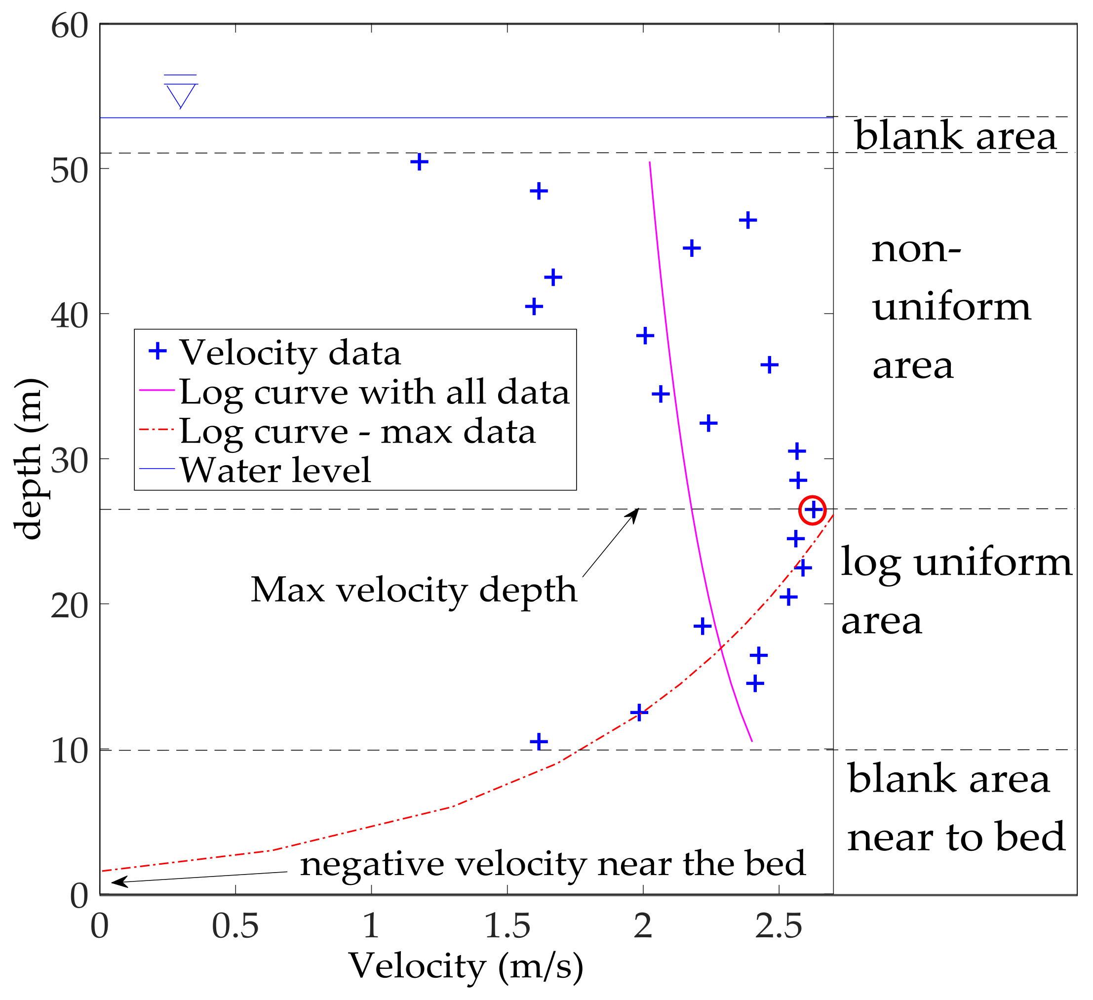
38] comment that the method does not hold in general and can only be considered an approximate representation of experimental data. For measurements at a single point, long time-series data are required for proper averaging. In the present study, the velocity distributions do not seem to follow a logarithmic profile, thus it was expected that this method is not applicable in detail.
Figure 4 shows a typical vertical profile of longitudinal velocities as measured in the canyon. The profile shows the features observed in the cross-section visualizations, with high velocities in deep channel regions. Unfortunately, the depth limitations of the equipment resulted in a large blanking region close to the bed. Regardless, the profile does not visually follow a log law. To minimize the velocity non-linearity problem, each velocity profile was separated in 2 parts: a non-uniform (near the water surface) and a log part (starting at the maximum velocity point in the profile). Using this assumption, only the data below the maximum velocity point were considered for the fitting processes. Several fits also resulted in negative velocities close to the bed, limiting this method further, thus not following it for the subsequent calculations.
3.3. Depth–Slope Product Method
The mean boundary shear stress equation considers a steady and uniform flow and is generally used in sediment transport studies to estimate the channel stability. In large rivers, with small slopes, it is possible to assume that the bed slope (S
0) is parallel to the energy slope (S
e) and the water level slope (S
ws), and the hydraulic radius (
Rh) nearly equals the transect-averaged water depth (<
h>). The application of these assumptions within the mean boundary shear stress equation is often referred to as the “depth-slope product”, as presented in:
where τ
0-ds is bed shear stress, by the depth-slope product method;
g is the gravitational acceleration (i.e.,
g = 9.81 m
2/s); <
h> is the transect-averaged water depth (m); S
e is the local energy slope. The transect-averaged water depth is a standard result of the ADCP measurement, and the bed slope (S
0) was considered equal to the water surface slope (S
ws) measured in the field. Because of the depth difference, the ADPC cross-section data were subdivided, selecting a mean hydraulic radius of the canyon area and another value for the rest of the cross-section. Unfortunately, the simplifications presented in the depth-slope product method (steady and uniform flow) are an unrealistic representation of the spatial data condition of the measurements in Lourenço’s Rock Canyon. Nonetheless, Sime et al. [
11] considered it worthwhile to compare the method with other results because of its high usability. However, it has not been followed further in this manuscript.
3.4. Boussinesq’s Hypothesis
The concept adopted in Reynolds averaging of the Navier–Stokes (RANS) created a non-linear term of the Navier-Stokes equation, called the “Reynolds stress”. The term represents the influence of the turbulent fluctuations in the momentum distribution in the mean flow [
39]. The coordinate system of the Reynolds stress is presented in
Table 1 [
40].
With the extra term, the equations of motion for turbulent flow can never form a closed system in which the number of equations is equal to the number of unknowns. This is called the turbulence closure problem and can be solved by eddy-viscosity models (EVM), which use Boussinesq’s hypothesis.
Boussinesq’s hypothesis was formulated in 1877 and is based on the analogous relationship between the viscous stresses of the laminar regime and the turbulent one, and it is assumed that the turbulent stresses are proportional to the mean velocity gradient of the flow in a similar manner as the viscous stresses (Newton’s Viscosity Law) [
41]. This proportionality factor was named the eddy viscosity (υ
t) and is not a physical property but is dependent on the current flow condition and turbulence levels. The correlation between the turbulent shear stress of the flow and the eddy viscosity (for the x and z coordinate axes) is described by:
where τ’
xz is the turbulent shear stress (x and z-axes), in kg/ms
2; <u’w’> is the Reynolds Stress component (x and z-axes); υ
t is the eddy viscosity, in m
2/s; k is the turbulent kinetic energy, in m
2/s
2; δ is the dimensionless Kronecker delta.
In natural rivers, the shear stress is the force of moving water against the bed, and the turbulent effects are the principal component (τ ≈ τ’). According to Vachtman and Laronne [
32], from the computed turbulent kinetic energy (k), based on the average of the velocity variances for a given depth above the bed, the tridimensional turbulent shear stress (τ’) can be estimated using [
13,
42]:
where C
1 is a dimensionless constant (i.e., C
1 ≈ 0.19–0.21). The specific value of C
1 may not apply at all levels within the water column because it requires confirmation before using the method universally [
13]. Nonetheless, this paper considered the turbulent shear stress for the water column (τ’
ensemble) equal to bed shear stress, by the TKE method (C
1 = C
0 = 0.20).
The velocity gradients and a 3D vorticity field were calculated using the ADCP velocity data. However, the transversal distance between the points was on average 1.5 m, and the longitudinal reached 200 m (distance between transects). Because of the longitudinal distance between the ADCP data, it is reasonable to set the terms with longitudinal distance to zero. Considering the vertical average and applying Boussinesq’s hypothesis, the turbulence eddy viscosity (for each ensemble) can be calculated as:
where υ
t ensemble is the turbulence eddy viscosity, in m
2 s
−1, τ’
ensemble is shear stress, by the TKE method (Nm
−2); ω
ensemble is the vertical average of the 3D vorticity along the cross-section (s
−1).
Numerical models are generally used to complement field data for further analysis. The most accessible and common models are Reynolds averaged Navier–Stokes (RANS) models, which require either the modeling or the definition of values for eddy viscosity. Usually, constant values are used, and simulations are calibrated using varying roughness values. However, under complex flow situations, the calibration process can result in non-realistic roughness coefficients, thus non-realistic results for simulations beyond the calibrated regime. Under such conditions, varying eddy viscosity values may provide better flow representations, as adopted in Cheng et al. [
39].
5. Discussion and Conclusions
The measured velocity profiles in the submerged canyon showed irregular flow features, characterized by high flow velocities in the deeper part of the canyon, and large secondary currents developing at the canyon side walls. Analyzing the sections velocity field, the higher vorticity values happened around the longitudinal axis. The initial processing of the data showed high velocity fluctuations in the vertical and transversal axis, representing the strong presence of turbulence along the canyon.
The turbulent quantities associated with the ADCP data indicated a large internal shear occurring within the canyon. Those effects have been summarized by computing the bed shear stress and eddy viscosity distributions and showing distinct regions with significant differences. The shear stress values from the depth–slope product method were considered lower than the real flow conditions, reaffirming the method limitations for high turbulence flow. The assumption used in the law of wall method assisted the curve-fitting process for non-logarithm velocity profiles. However, because of the blank area near the bottom, some curves were fitted considering negative velocities near the bottom, resulting in higher values for the bed shear stress along the canyon and some outside parts. The results from the TKE method were considered most realistic for the canyon area, with shear stress values similar to those presented in other studies with similar conditions [
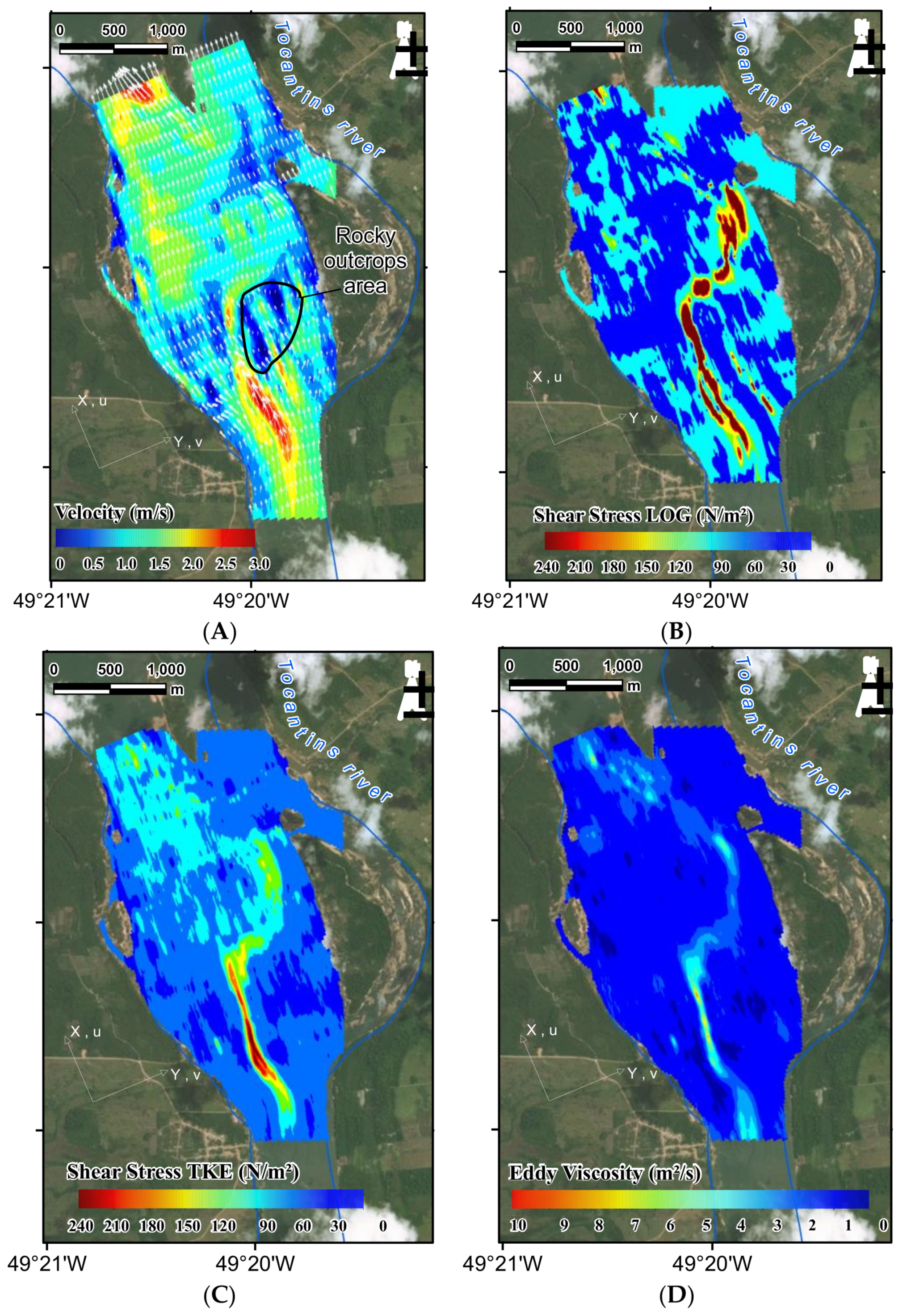
13]. The most significant shear stress difference happened in the canyon upstream, with values 8 times greater than outside.
The eddy viscosity distributions show reasonable results with values around the regular 1.0 m2/s used for rivers. In most of the areas of the stretch, the values were between 0.8 and 1.8 m2/s. In the canyon, analyzing each section, some points reached values higher than 20 m2/s. For spatial analysis, the higher value considered was 10 times higher than the other parts of the stretch.
The spatial interpolation was able to show the horizontal variation of shear-stress and eddy viscosity distributions. However, due to the longitudinal distance between the cross-sections, it was not possible to represent the velocity gradients at the x-direction (∂<v>/∂x and ∂<w>/∂x).
The turbulent quantified values can be used with the intention to improve hydrodynamic numerical model calibrations (turbulence models) and better representation of physical processes. However, it is important to highlight the assumptions and the methodology limitations described in this paper, such as the short velocity time series and the interpolation.
To improve future field measurements, we recommend adding extra points with fixed ADCP measurements along each section to evaluate the shear stress results with an extensive time series. To improve the vertical analysis, equipment with a different frequency to check the velocity near the bottom should be used. For longitudinal analysis, the maximum distance should be only 2 times the transversal distance data.
For future analysis, a sensitivity grid test is recommended, comparing different cell sizes or applying a non-regular grid. In addition, different interpolation methods can be tested. The next steps will be to compare the results of the flood and drought season (already measured, but not processed) and to evaluate their applicability to hydrodynamic models.


