Next Article in Journal
Swimming Pool Evaporative Water Loss and Water Use in the Balearic Islands (Spain)
Previous Article in Journal
Water Resources and Sustainability Assessment Based on Group AHP-PCA Method: A Case Study in the Jinsha River Basin
 
 
Correction published on 9 October 2019, see Water 2019, 11(10), 2099.
Article

Study on the Applicability of the Hargreaves Potential Evapotranspiration Estimation Method in CREST Distributed Hydrological Model (Version 3.0) Applications

1
State Key Laboratory of Hydroscience and Engineering, Department of Hydraulic Engineering, Tsinghua University, Beijing 100084, China
2
State Key Laboratory of Simulation and Regulation of Water Cycle in River Basin, Research Center on Flood & Drought Disaster Reduction of the Ministry ofWater Resources, China Institute of Water Resources and Hydropower Research, Beijing 100038, China
3
School of Civil Engineering and Environmental Science, University of Oklahoma, Norman, OK 73019, USA
*
Authors to whom correspondence should be addressed.
Water 2018, 10(12), 1882; https://doi.org/10.3390/w10121882
Submission received: 6 November 2018 / Revised: 7 December 2018 / Accepted: 17 December 2018 / Published: 19 December 2018
(This article belongs to the Section Hydrology)

Abstract

:
The potential evapotranspiration (PET) is an important input to the hydrological model and its compatibility has an important influence on the model applications. The applicability of the Hargreaves-Samani (HS) PET estimation method in Coupled Routing and Excess STorage distributed hydrological model version 3.0 (CREST 3.0 model) was studied in a typical humid region, Ganjiang River Basin, in Southern China. The PET estimation methods were evaluated based on the streamflow simulation accuracies using the CREST 3.0 model driven by different PET products with various spatial resolutions. The Penman-Monteith (PM) equation-based PET estimation method was adopted as the reference PET estimation method in this study. The results demonstrated that PET obtained from the HS method was larger than that generated by the PM method, and the CREST 3.0 model driven by both HS and PM-based PET products can simulate the streamflow temporal variations equally well in annual time scale. Compared with the PM method, the HS method was more stable and robust in driving CREST 3.0 model under the scenarios of different spatial resolutions. In addition, during the validation period (2007–2009) with 2003–2006 as the calibration period, the HS outperformed PM considering the streamflow simulation accuracy. Therefore, the HS method was not only applicable to CREST 3.0 model with flexible spatial resolutions, but also can be an alternative method to PM method in CREST 3.0 model streamflow simulation applications in Ganjiang River Basin. The study results will not only increase the confidence on the applicability of the HS method in hydrological simulation in Ganjiang River Basin, but also prove the flexibility of CREST 3.0 model in terms of PET input, which will expand the application range of the CREST 3.0 model.

1. Introduction

Potential evapotranspiration (PET), which is defined as the maximum possible evapotranspiration rate under the condition of sufficient soil water availability [1], is a vital flux for hydrological processes and is an important input to the hydrological model applications [2,3]. A flexible and reliable PET input could greatly facilitate the application of the hydrological model.
Numerous methods have been proposed to estimate the PET in past decades. It can be estimated either by using land-atmosphere energy balance aerodynamics principles or by empirically determined methods [4,5,6,7]. The FAO-56 PM, a standard version of the classic Penman-Monteith (PM) equation recommended by Food and Agriculture Organization (FAO), is the most widely used PET estimation method and is usually regarded as the best method to provide the most accurate PET information [5]. As a physically-based land-atmosphere energy balance model, FAO-56 PM requires lots of input variables including air temperature, relative humidity, solar radiation, and wind speed. Thus, its applicability is often restricted by the availability of the climate variables in real-world applications. Therefore, the empirical methods, such as Hargreaves (HS) method [6,8], Thornthwaite (TH) method [9,10], Priestley-Taylor equation [7], Blaney-Criddle method [11], Jensen–Haise [12], and Hamon method [13,14], are widely adopted as PET estimators since they only need a few widely available climate variables such as air temperature. Considering the reliability and availability of the climate variables, empirical methods, especially the temperature-based ones, may be better options in scenarios such as PET estimation in data-lacked areas and future PET projection.
Among temperature-based PET estimation methods, the Hargreaves-Samani method (HS) [8] and TH method [9,15] are two widely used approaches, especially in the research fields of hydrological, agricultural, and ecological models. Compared with the classic TH method, HS method requires the daily minimum and maximum air temperatures as input data rather than just adopting mean air temperature by the TH model. Therefore, HS model not only gets the atmospheric mean status through the mean air temperature, but also partly captures the land surface property information, such as soil moisture and land surface albedo by introducing diurnal temperature range [16]. From this aspect, HS is more reasonable than TH method. Moreover, enhancement of the atmospheric evaporative demand has taken place under the scenario of global warming [17]. Therefore, the PET method must have the ability to capture the global warming information in the hydrological projection applications. Compared with the TH model, the character of asymmetric warming rate for the daily maximum/minimum temperature can be reflected by the HS model. Thus, HS is more applicable than TH in PET estimation under climate change scenario. Therefore, HS method has been widely evaluated and applied across different climate regions [18,19].
Though the above-mentioned analyses show that the HS methods are more suitable for PET estimation than TH, the compatibility and applicability of the HS method in hydrological model should be further verified by validating the model simulation performance in applications. Some previous literatures have involved in the comparison of applicability of different PET estimation methods in hydrological simulation, concerning PM, HS, TH, and other methods [20]. However, until recently, they have not yet reached a consensus with regard to the relationship between the hydrological model performance and the PET estimation method. For example, several researchers reported that hydrological models appear to be insensitive to different PET inputs in term of streamflow simulation [2,21,22]. While other results showed that the accuracy of the streamflow simulation is significantly impacted by different PET inputs [23,24]. It should be noticed that the conflicting conclusions are possibly caused by the adoption of different hydrological models. For example, based on four conceptual rainfall–runoff models, Oudin et al. got the conclusion that both empirical and complex PM methods can achieve similar model performance [25]. Bai et al. [20] also confirmed this opinion by using two monthly hydrological models, the Wang model [26] and another model proposed by Thomas [27] in China. While based on Système Hydrologique Européen (SHE) model (MIKE-SHE v5.30, Danish Hydraulic Insititue, Hørsholm, Denmark), Vázquez et al. found that different PET inputs had significant impacts on the accuracy of streamflow simulation [24]. Thus, we belive the sensitivity of PET to hydrological streamflow simulation is largely depending on the structure of the adopted hydrological models. Therefore, as to the specific hydrological model, the applicability of the HS method should be further verified by driving the specific hydrological model and comparing the streamflow simulation accuracy.
The conceptually-based distributed hydrological model, Coupled Routing, and Excess STorage (CREST) model (1.0, University of Oklahoma, Norman, OK, USA) has been widely applied across different basins [28,29,30]. As a vital input of the CREST model, PET plays an important role in the runoff generation process and water balance. Gan et al. studied the CREST model and evaluated the impact of parameter KE (a parameter closely related to PET) on streamflow simulation across various watersheds over China by using daily PET which was acquired from the Famine Early Warning Systems Network, FEWS (it is generated using the PM equation) [31]. Their results indicate that KE is a sensitive parameter and its sensitivity varies across different watersheds. It is more sensitivie over the basins in Northeast China [31]. The results partly provided that the PET dataset is an important and sensitive input for CREST model simulation. However, there is no report concerning the applicability of different PET estimation methods applied to the CREST model simulation. Furthermore, considering the spatial scale difference between the resolution of the PET products and the grid size of the hydrological model, the scale effect of PET to CREST model simulation also needs to be investigated.
In order to explore the applicability of HS method in hydrological simulation, especially for CREST model, we adopted a new version CREST model (CREST Version 3.0) [30] in this study. Based on the CREST 3.0 model, the hydrological assessments of HS estimated PET with PM-based PET as a reference were performed in a typical humid region, Ganjiang River Basin. This work aims to provide useful guidelines to the users of the CREST 3.0 model and enhances the understanding of the CREST model behaviors.
This paper is organized as follows: The study area and data are presented in Section 2. The two PET estimation methods, CREST model, and CREST simulation experiment designs are described in Section 3. In Section 4, the results and discussion are presented. Finally, conclusions and future perspectives are given in Section 5.

2. Study Area and Data Description
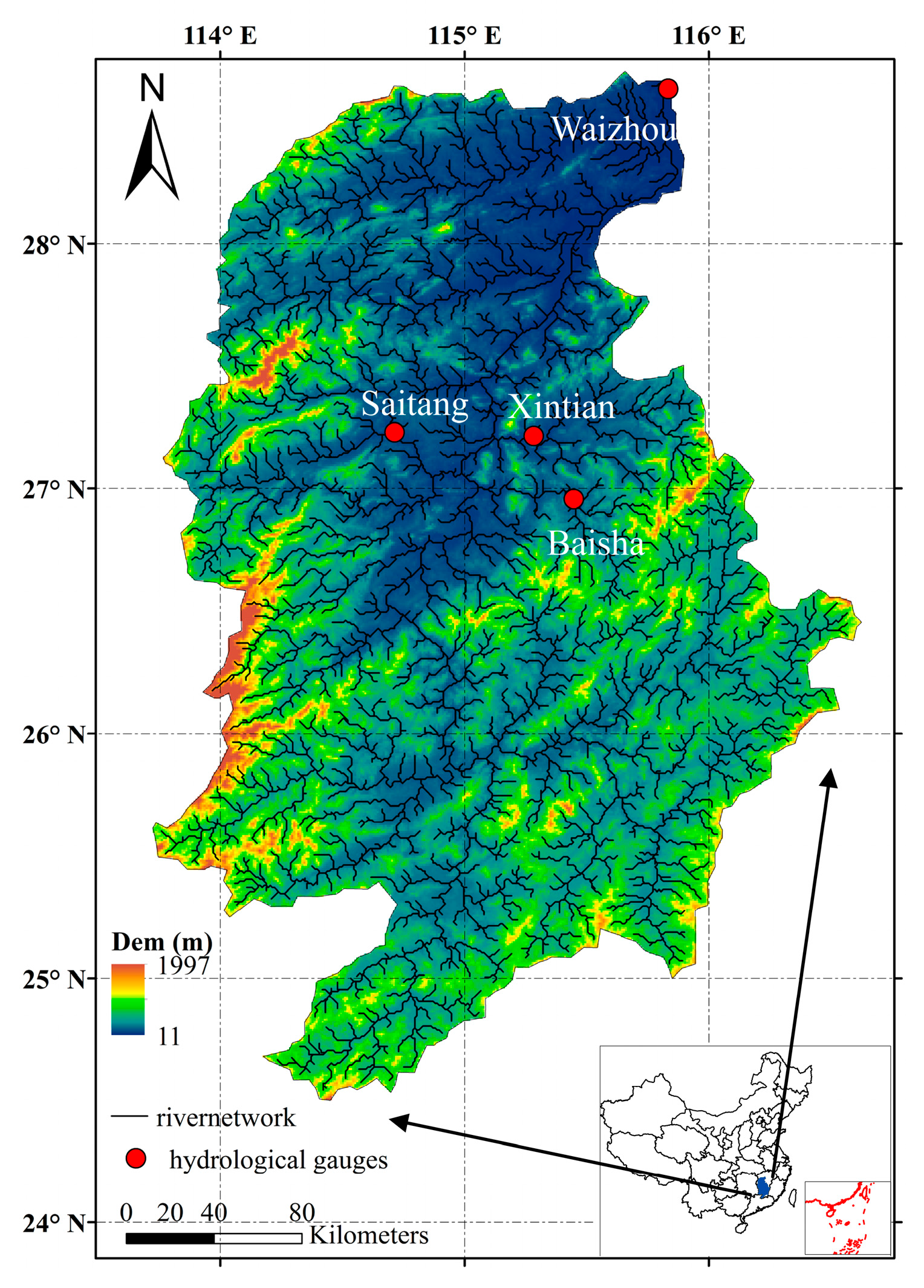
2.1. Study Area

The Ganjiang River Basin, which is located in the Southeast part of China, was selected as the case study area (Figure 1). It is the tributary of the Yangtze River and is the longest river in Jiangxi Province. Extended from 113.5° E to 116.6° E and 24.5° N to 29.18° N, the Ganjiang River Basin has a drainage area of 81,258 km2 above the Waizhou hydrological station. The elevation of the Ganjiang River Basin ranges from 11 m to 1997 m and the terrain varies significantly from hilly land to low hill. The long term annual precipitation and temperature are 1580 mm and 18.3 °C, respectively. The subtropical humid monsoon climate predominates over this region, thus most rainfall falls in April and June, thereby resulting in floods [32].

2.2. Data

The data required by the CREST 3.0 model (3.0, Tsinghua University, Beijing, China) mainly includes the rainfall and PET forcing data combined with the observed historical streamflow data. Other underlying surface data such as digital elevation model (DEM), land cover, soil type data, etc., are also needed.
In order to eliminate the influence of forcing data on this study, two different widely used datasets, the China Meteorological Forcing Dataset, which was developed by Data Assimilation and Modeling Center for Tibetan Multi-spheres, Institute of Tibetan Plateau Research, Chinese Academy of Science (http://westdc.westgis.ac.cn/data/7a35329c-c53f-4267-aa07-e0037d913a21) (ITPCAS data), and Meteorological forcing datasets provided by Land-Atmosphere Interaction Research Group at Beijing Normal University (BNU data) from 2003–2009 were employed in this study. The ITPCAS has a spatial resolution of 0.1° and 3-hourly temporal resolution, which was produced by merging reanalysis data, remote sensing data, and ground station observations in China. It has been evaluated and applied to study the land-atmospheric interaction in China [33,34,35,36]. Detailed information can be found in He et al. [37]. The BNU data is a ground-based gridded dataset with the spatial-temporal resolutions of 0.05° and 3-hourly, which is interpolated based on about 700 stations of the Mainland China [38,39]. This forcing data was produced to drive the land surface model over China, which is characterized with its high spatial resolution. The forcing data variables, including temperature, surface pressure, relative humidity, and downward shortwave/longwave solar radiation were adopted to generate the PET dataset by using the HS and PM methods.
For the purpose of performance comparison of different PET products with various spatial resolutions and different inversion algorithms, the forcing data of the ITPCAS and BNU from 2003–2005 was resampled to 10 km, 25 km, and 100 km, respectively, by bilinear interpolation method. PET data was then generated from the interpolated forcing data by using different PET estimation methods. The PET datasets were reorganized into 12 sub-sets (see in Table 1):
For the purpose of hydrological simulation performance comparison between HS and PM methods in the CREST version 3.0, two datasets (a, PET with 25 km spatial resolution generated from ITPCAS forcing dataset using HS method; b, PET with 25 km spatial resolution generated from ITPCAS forcing dataset using PM method) from 2003 to 2009 were produced to perform the comparison and evaluation.
The rainfall data from 2003 to 2009 came from the Tropical Rainfall Measuring Mission (TRMM) satellite-based remote sensing product 3B42V7 (3B42V7, National Aeronautics and Space Administration, NASA, Washington, DC, USA). The original spatial-temporal resolutions of the TRMM 3B42V7 rainfall data are 0.25° × 0.25° and 3-hour, respectively. It was resampled into the same spatial resolution corresponding to Table 1 and daily scale by using the nearest-neighbor method and daily rainfall accumulation.
The daily streamflow data for model parameter calibration and model performance intercomparison were obtained from observations of the Baisha, Saitang, Xintian, and Waizhou stations (see in Figure 1). The streamflow data ranges from 1 January 2003 to 31 December 2009 and the data time interval is one day.

3. Methodology

3.1. Penman-Monteith Method

As a typical classic physically-based PET estimation method, PM is regarded as the most reliable method to generate PET under distinct climatic conditions [40,41]. Therefore, PET calculated by the PM method is usually used as the reference or benchmarking to evaluate other PET estimation methods [3,42]. FAO56-PM PET is calculated as follows:
E 0 = 0.408 Δ ( R n G ) Δ + γ ( 1 + 0.34 U 2 ) + γ 900 T m e a n + 273 U 2 ( e s a t e a ) Δ + γ ( 1 + 0.34 U 2 )
where Δ is the slope of saturated vapor pressure (kPa·C−1); Tmean is the daily mean air temperature at 2 m height (°C), which can be obtained by 0.5(Tmax + Tmin); Tmax and Tmin are the daily maximum and minimum air temperature, respectively; γ is the psychrometric constant (kPa·C−1); Rn is the net radiation (MJ·m−2·day−1); G is the downward ground heat flux (MJ·m−2·day−1), it is usually considered as zero at daily time scale; and esat and ea are the saturated and actual vapor pressures (kPa), respectively. U2 is the wind speed at 2 m height (m/s).

3.2. Hargreaves Method

Hargreaves method, proposed by Hargreaves [6], is also named Hargreaves-Samani (HS) equation method. The HS method is the most commonly used temperature-based method and is recommended by FAO as an alternative method for PET estimation when observed weather data are unavailable [5]. The HS method estimate PET as follows:
E T H S = k R S   · R a · ( T m a x T m i n ) H E ( T m a x + T m i n 2 + H T )
where ETHS is daily PET in mm·day−1; Ra is extraterrestrial radiation in mm·day−1; Tmax and Tmin are daily maximum and minimum air temperature in °C, respectively; kRS is the empirical radiation adjustment coefficient and the value is set to 0.0023 in this study; HE is empirical Hargreaves exponent and the value is set to 0.5 in this study; and HT is empirical temperature coefficient and the value is set to 17.8 in this study [43].

3.3. CREST Distributed Hydrological Model Version 3.0

The CREST model is jointly developed by the University of Oklahoma and NASA SERVIR (SERVIR, a joint venture between NASA and the U.S. Agency for International Development, provides state-of-the-art, satellite-based Earth monitoring data, geospatial information and tools to help improve environmental decision-making among developing nations). It is a conceptually-based distributed hydrological model which is developed to simulate the spatial and temporal variations of the land surface, subsurface water fluxes and storages by cell-to-cell simulation. CREST’s distinguishing characteristics include: (1) Distributed rainfall–runoff generation and cell-to-cell routing; (2) coupled runoff generation and routing via three feedback mechanisms; and (3) representation of sub-grid cell variability of soil moisture storage capacity and sub-grid cell routing (via linear reservoirs). The coupling between the runoff generation and routing mechanisms allows detailed and realistic treatment of hydrological variables such as soil moisture. Furthermore, the representation of soil moisture variability and routing processes at the sub-grid scale enables the CREST model to be readily scalable to multi-scale modelling research at local, regional, and global scopes.
The CREST model was initially designed to provide real-time regional and global hydrological predictions by simultaneously modeling over multi-basins with significantly cost-effective computational efficiency [28], but it is also applicable for small to medium size basins at very high-resolutions [29,44]. CREST simulates the spatiotemporal variations of water fluxes and storages on a regular grid with the grid cell resolution being user-defined, thereby enabling multi-scale applications. The scalability of the CREST model is accomplished through sub-grid scale representation of soil moisture storage capacity (using a variable infiltration curve) and multi-scale runoff generation processes (using multi-linear reservoirs). The representation of the primary water fluxes such as infiltration and routing are physically related to the spatially variable land surface characteristics (i.e., vegetation, soil type, and topography, etc.). The runoff generation process and routing scheme are coupled, thus providing more realistic interactions between lower atmospheric boundary layers, terrestrial surface, and subsurface water. The above flexible modeling features and embedded automated calibration algorithms make the CREST a powerful yet cost-effective tool for distributed hydrological modeling and implementation at global, regional, basin, and small catchment scales.
The version history of the CREST model can be traced back to the original 1.x version developed by Wang et al. in 2011 [28]. After that, the model is continuously updated from CREST 1.6c to modular designed 2.0 Fortran version with embedded SCE-UA (Shuffled Complex Evolution, developed at University of Arizona) automatic parameter optimization by Xue et al. [44]. Until recently, the Fortran version has been updated to 2.1 and has been successfully applied regionally and globally. In addition to the Fortran version, there is another CREST 2.1 implementation by using MATLAB (a mathematical computational software developed by MathWorks Corporation) and GDAL (Geospatial Data Abstraction Library) libraries with additional input/output functionalities. The 2.0 and 2.1 are noted as 2.x for simplicity in this paper.
The CREST has been widely applied in hydrological studies [32,44,45,46] and successfully implemented in several flood warning systems including the Flooded Locations And Simulated Hydrographs Project (FLASH; http://blog.nssl.noaa.gov/flash/) and the Global Flood Monitoring System (GFMS; http://eos.ou.edu). Recently, a new version CREST had been published by Kan et al. [30]. CREST V3.0 made four improvements to the traditional CREST 2.x model:
  • Separating the soil layer into three layers and consider 3-layer tension water soil moisture and evapotranspiration computations.
  • Adding a free water storage computation module with a free water distribution curve to describe the sub-grid variations of the free water storage.
  • According to free water storage, separating runoff into three components, including overland flow, interflow, and ground water.
  • Improving the flow concentration module into a four mechanisms-based cell-to-cell routing, including overland flow, interflow, ground water, and river channel flow routings. Based on the arrival time of each upstream grid cell to its downstream outlet grid cell, the generated runoff is routed down along the flow concentration path generated according to the 8-flow-direction method.
The CREST 3.0 model [30,47] has also been successfully applied in Ganjiang River Basin, China to verify the characteristics of model calibration, simulation, and validation. The above-mentioned improvements make the CREST model easier to combine with the remotely-sensed data such as soil moisture and actual evapotranspiration to decrease the uncertainty problems in distributed hydrological model calibration and validation, and the give possibility to improve the model simulation capability in regional and global applications. In this study, CREST version 3.0 was employed to evaluate the applicability of HS method.

3.4. The Design of the Numerical Experiment

According to the objective of this study, two groups of numerical experiments were designed as follows:
Experiment 1: In order to perform evaluation of spatial scale effect of different PET products on CREST model performance, PET estimated from BNU, and ITPCAS meteorological data sources by using HS and PM estimation methods at 10, 25, and 100 km spatial scales were used to drive the CREST model. The CREST model was ran during the period 2003 to 2005. The data from 2003 to 2004 was treated as calibration period and data of 2004 was treated as a validation period. The PET data was classified into 12 sub-datasets according to different meteorological data sources (BNU and ITPCAS), spatial scales (10, 25, and 100 km), and estimation methods (HS and PM methods) (see in Table 1).
Experiment 2: For the purpose of the performance comparison between HS and PM methods for the CREST model streamflow simulation, two datasets (a, PET with 25 km spatial resolution generated from ITPCAS forcing dataset using HS method; b, PET with 25 km spatial resolution generated from ITPCAS forcing dataset using PM method) from 2003 to 2009 were produced to perform the comparison and evaluation. The data spanning from 2003 to 2006 was used for model calibration and the dataset from 2007 to 2009 was used for model validation.
In both of the two experiments, the simulated streamflow was compared against observed streamflow at the basin outlet station, i.e., the Waizhou station.

3.5. Statistical Metrics

To quantitatively evaluate the hydrological simulation performance of the CREST model driven by different PET datasets, several widely used performance metrics were adopted in this study. The correlation coefficients (CC) describes the agreement between the simulated and observed streamflow. The relative bias (BIAS) and the root mean square error (RMSE) were used to describe the error and bias of the CREST simulation compared with the observed discharge. In addition, a comprehensive index, the Nash-Sutcliffe coefficient efficiency (NSCE) is adopted to assess the overall streamflow simulation performance of the CREST model (see Table 2).

4. Results and Discussion

4.1. Intercomparison of Daily PET Among Two Datasets

Two datasets (ITPCAS-25 km-HS and ITPCAS-25 km-PM) were employed to investigate the spatial discrepancy between two PET estimation methods over Ganjiang River Basin. The spatial distribution of average annual total PET is presented in Figure 2. There is a huge spatial difference between two datasets, not only in terms of spatial pattern, but also in terms of magnitude. As shown in Figure 2, ITPCAS-PM result varies from 750 mm/year to 1100 mm/year, while ITPCAS-HS result ranges from 800 mm /year to 1200 mm/year. For two datasets, the hilly region in the West of the basin, which is around 26° N and 114° E, has the lowest annual PET. However, the highest value of annual PET for the ITPCAS-HS is located in the Southeast of the basin while for the ITPCAS-PM being in southwest of the basin.
The basin regional mean daily PET from 2003 to 2009 is shown in Figure 3. Though both of the two datasets could satisfactorily reproduce the annual temporal variation in a daily cycle. However, the magnitude of regional mean PET of HS model is significantly higher than that of PM.

4.2. Spatial Scale Effect of Pet to The Streamflow Simulation Based on CREST 3.0 Model

Based on experiment 1, the spatial scale effect of PET on CREST 3.0 streamflow simulation is investigated by comparing the CREST simulated streamflow with that observed in 2005 with 2003–2004 as the calibration period.
As shown in Table 3, at the scale of 100 km (about 1 degree), the performance of HS outperformed PM in term of all the metrics except for the BIAS. It is noted that for the PM dataset, both BNU and ITPCAS 100 km datasets showed the negative bias and larger RMSE in each group, i.e., −3.04% and 1237.51 m3/d and −2.13% and 1328.21 m3/d, respectively.
At 10 km and 25 km scales, there is no significant difference between PM and HS model in both ITPCAS and BNU datasets in terms of CC, BIAS, and NSCE. Additionally, the 25 km scale PET for both of BNU and ITPCAS datasets show better performance with lower BIAS and RMSE, as well as higher CC and NSCE.
We use standard derivation (STD) of statistical metric to analyze the stationarity of the CREST model performance with different spatial resolutions of PET (in Table 4). The lower STD of metric represents the lower sensitivity and higher stability for the PET estimation method applied in the CREST 3.0-based streamflow simulation.
In general, the statistical metrics, including NSCE, CC, and RMSE indicate that the stability of CREST with BNU dataset is higher than that of ITPCAS. This result could be attributed to the different original spatial resolution of the two meteorological forcing datasets. As the spatial resolution of BNU dataset is about 5 km, while ITPCAS is about 10 km. Therefore, BNU dataset contains more spatial information compared with ITPCAS dataset to generate better PET products.
As far as different PET estimation methods are concerned, the HS showed lower STD of metrics for two meteorological forcing data, indicating that the sensitivity of CREST to the scale effect of HS is relatively lower than that of PM method. In other words, in CREST model, HS outperformed PM in terms of scale effect.
The different sensitivities of CREST to PET method probably come from the uncertainties contained in different meteorological forcing inputs. As mentioned above, the PM method needs detailed atmospheric information, including air temperature, humidity, wind speed, air pressure, and downward radiation. Theoretically speaking, the more environment information considered in the model, the more precise the PET results would be. However, besides the uncertainty of variables themselves, the atmospheric variables have different spatial scale characteristics, e.g., the heterogeneity of wind speed is obviously larger than that of air temperature. The scale effect of different variables would bring more uncertainties to the PET estimations. In contrast, the HS method only requires daily minimum/maximum air temperature, which is relatively insensitive to spatial scale. Thus, there will be less variations for the HS in different spatial resolutions. Therefore, the HS is more robust in comparison with the PM method considering different spatial scales.

4.3. Comparison of Model Performance between PM and HS Methods in Streamflow Simulations (2003–2009)

In order to compare model performance between PM and HS estimation methods in streamflow simulations, we adopt dataset of 2003–2006 as the calibration set and dataset of 2007–2009 as the validation set. For the validation period of 2007–2009, the simulated streamflow (see in Figure 4 and Table 5) forced by HS estimated PET showed better agreement with the observations and can capture most of streamflow peak flows compared with that based on PM PET estimation. As Table 4 shows, HS-based CREST had higher CC and NSCE (0.74 and 0.37, respectively) and lower BIAS and RMSE (6.81% and 1163.65 m3/s), indicating that the performance of HS method was better.
Due to its clear physical concepts, PM method has received wide acceptance and has been applied over various climate regions in ecology, agriculture irrigation, and hydrology related research fields. However, the comparison of streamflow simulation accuracy evaluations between PM and HS in the CREST 3.0 model showed that the performance of PM method was not as good as expected. In contrast, the HS outperformed PM in CREST 3.0 model applications.
The above-mentioned results are consistent with previous studies. Andersson et al. reported that the temperature based statistical ET model (Thornthwaite) showed a better hydrological adaptability than PM method [22]. In the work of Andréassian et al., their results showed that a perfect ET did not mean a better hydrological model performance [2]. Oudin et al. assessed 27 ET models in a daily rainfall–runoff model over 308 catchments, and also drew a similar conclusion [25]. Kannan et al. illustrated that the streamflow simulation driven by HS was much better than that of PM in the Soil & Water Assessment Tool (SWAT)-2000 model (Version 2000, Texas Water Resources Institute, Texas, TX, USA) [48]. Bai et al. also indicates that the performance of HS is similar to that of PM in term of streamflow simulation in arid and humid basins [20].
For the reason of the mediocre performance of the PM method in the hydrological model, the researchers also try to give a reasonable explanation. For example, Burnash (1995) pointed out that an average annual evapotranspiration curve appears to be more meaningful in the watershed model [49]. Oudin et al. argued that the tolerant capability of hydrological model eliminates the precious of PM estimation method [50]. The opinion of Zhao et al. [51] was that the physical scale of hydrological modelling was still larger than that of the PM method, and thus the uncertainty of the soil moisture function in hydrological model constrains the advantage of the PM method. However, this question still needs further investigation.
While the HS method is developed over arid grassland [6], and is more applicable over arid and semi-arid regions, the good performance of HS PET over the typical humid region, Ganjiang Basin, showed that it is likely to be also applicable to humid basins with similar climate conditions as the Ganjiang River Basin.

5. Conclusions

This study investigated the applicability of HS method in CREST model version 3.0. Two groups of numerical experiments were conducted to evaluate the hydrological applicability of the classic PM method (FAO56-PM) and the HS method in CRSET V3.0 streamflow simulation over Ganjiang River Basin.
The research results are summarized as follows:
(1)
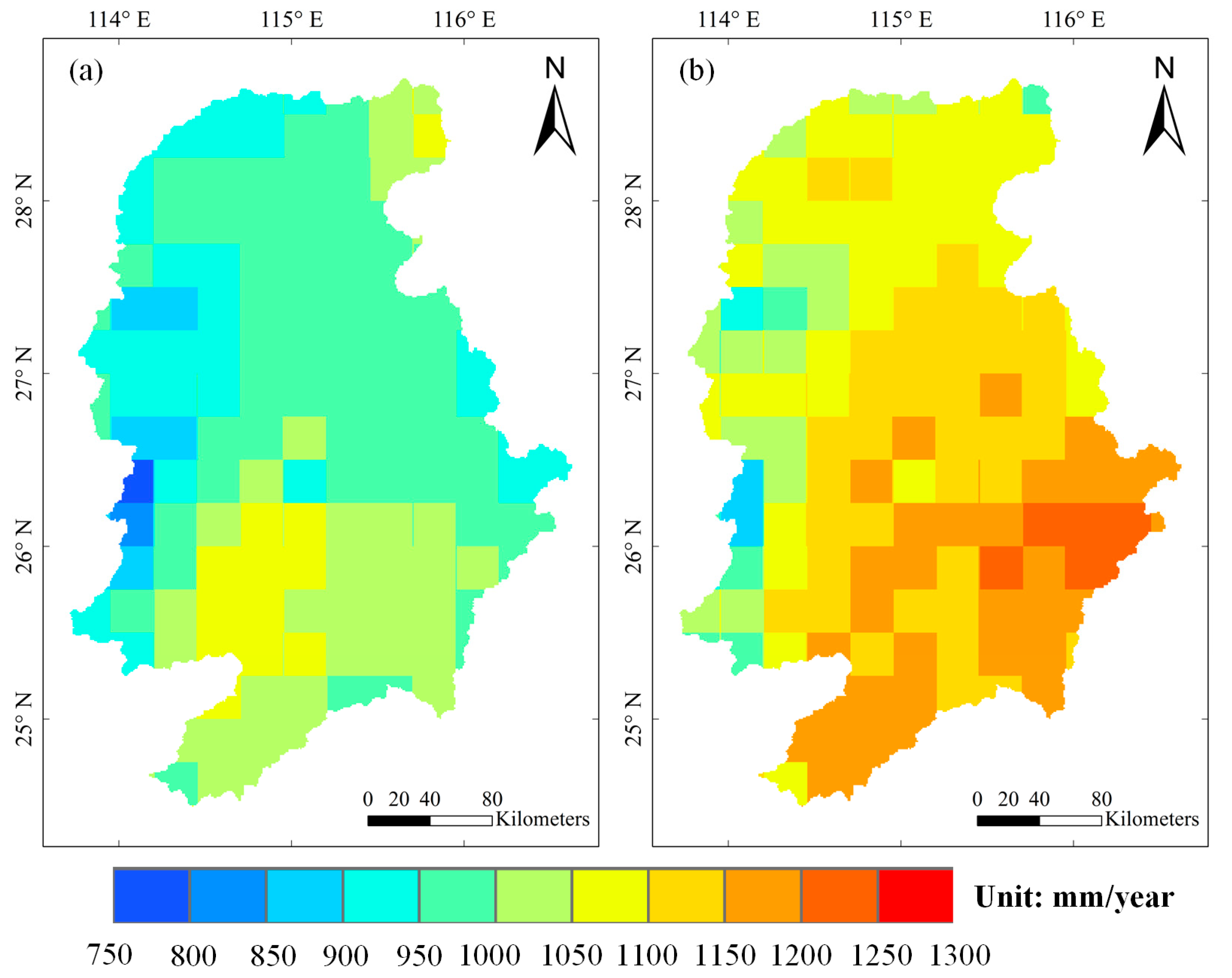
The PET estimated by the PM and HS methods show large difference in spatial distribution. Two PET estimations are consistent in the lowest PET region, but vary much over the region with relatively high PET magnitude.
(2)
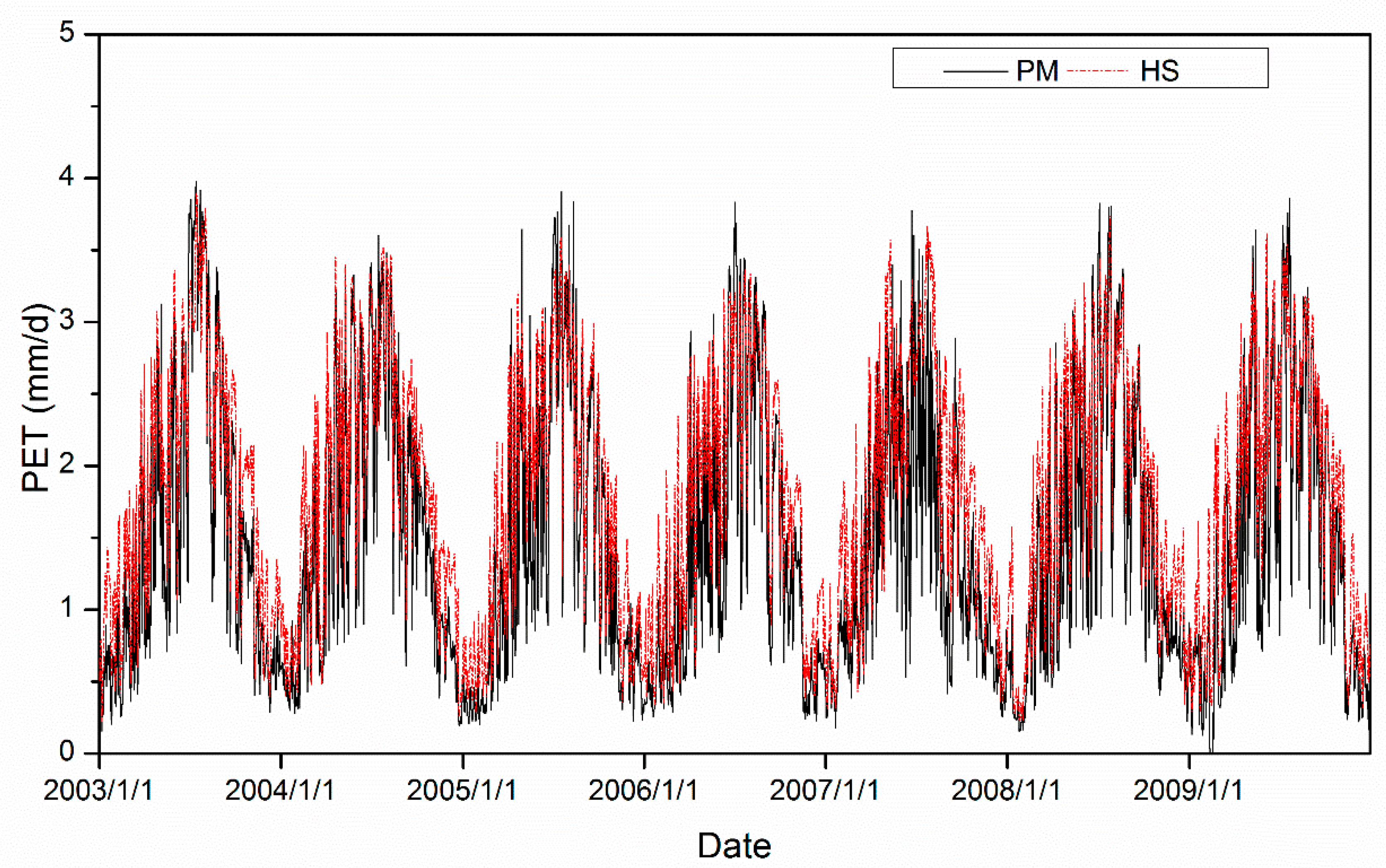
Two PET methods can reproduce the annual variations of the PET on daily time scale, but the magnitude of HS is higher than that of PM.
(3)
There is no significant discrepancy between HS and PM methods in CREST-based streamflow simulations with the same spatial scale by using BNU and ITPCAS meteorological forcing datasets. The BIAS and RMSE indicates that the performance of CREST model with 25 km spatial resolution is better than 10 km and 100 km.
(4)
Standard derivation (STD) of statistical metric for CREST model with PET products of different spatial resolutions indicates that the sensitivity of CREST model to the spatial scale of HS estimates is relatively lower than that of PM in the Ganjiang River Basin.
(5)
The comparison of hydrological simulations with 25 km ITPCAS data shows that the HS outperforms PM in streamflow simulation in this study area.
The results of this study show that the CREST model is more insensitive to the spatial scale of HS estimates than PM. The CREST model with HS-estimated PET performs better than that with PM considering the streamflow simulations in Ganjiang River Basin.
Therefore, we conclude that the HS can be an alternative to the classic PM method in the CREST 3.0 model over Ganjiang River Basin. This is important for the CREST 3.0 model users because the application scope of CREST 3.0 model can be extended owing to the flexibility of the PET input. Results in this study may be specific to the Ganjiang River Basin, but are likely to also be applicable to other humid basins with similar hydrological-meteorological conditions. This conclusion will be explored in our future studies. Besides, The HS method is most applicable in arid regions. However, the PET method applicability does not mean hydrological suitability, and therefore, the HS applicability in CREST 3.0 model in the arid and semi-arid regions still needs to be investigated.

Author Contributions

Z.L., G.K., and Y.H. designed this study; Z.L. and Y.Y. processed and provided the data; G.K. run the hydrological model; Z.L. wrote this manuscript; Y.Y. and G.K. modified and polished this manuscript.

Funding

This research was funded by Natural Science Foundation of China, grant number 71461010701 and 41701385; Beijing Natural Science Foundation, grant number 8184094; IWHR Research & Development Support Program, grant number JZ0145B022018.

Acknowledgement

The authors wish to extend appreciation to Land-Atmosphere Interaction Research Group at Sun Yat-sen University for providing meteorological forcing dataset (BNU dataset) (http://globalchange.bnu.edu.cn/research/data) and Cold and Arid Regions Science Data Center at Lanzhou (http://westdc.westgis.ac.cn) for providing meteorological forcing dataset (ITPCAS dataset). We are very grateful to the editors and anonymous reviewers for their critical comments and thoughtful suggestions.

Conflicts of Interest

The authors declare no conflict of interest.

References

  1. Wang, Z.; Xie, P.; Lai, C.; Chen, X.; Wu, X.; Zeng, Z.; Li, J. Spatiotemporal variability of reference evapotranspiration and contributing climatic factors in China during 1961–2013. J. Hydrol. 2017, 544, 97–108. [Google Scholar] [CrossRef]
  2. Andréassian, V.; Perrin, C.; Michel, C. Impact of imperfect potential evapotranspiration knowledge on the efficiency and parameters of watershed models. J. Hydrol. 2004, 286, 19–35. [Google Scholar] [CrossRef]
  3. Vicente-Serrano, S.M.; Azorin-Molina, C.; Sanchez-Lorenzo, A.; Revuelto, J.; López-Moreno, J.I.; González-Hidalgo, J.C.; Moran-Tejeda, E.; Espejo, F. Reference evapotranspiration variability and trends in Spain, 1961–2011. Glob. Planet. Chang. 2014, 121, 26–40. [Google Scholar] [CrossRef] [Green Version]
  4. GaviláN, P.; EstéVez, J.; Berengena, J.N. Comparison of Standardized Reference Evapotranspiration Equations in Southern Spain. J. Irrig. Drain. Eng. 2008, 134, 1–12. [Google Scholar] [CrossRef]
  5. Allen, R.G.; Pereira, L.S.; Raes, D.; Smith, M. Crop Evapotranspiration-Guidelines for Computing Crop Water Requirements-FAO Irrigation and Drainage Paper 56; FAO: Rome, Italy, 1998; Volume 300, p. D05109. [Google Scholar]
  6. Hargreaves, G.H. Estimating Potential Evapotranspiration. J. Irrig. Drain. Div. ASCE 1982, 108, 225–230. [Google Scholar]
  7. Priestley, C.; Taylor, R. On the assessment of surface heat flux and evaporation using large-scale parameters. Mon. Weather Rev. 1972, 100, 81–92. [Google Scholar] [CrossRef]
  8. Hargreaves, G.H. Accuracy of estimated reference crop evapotranspiration. J. Irrig. Drain. Eng. 1989, 115, 1000–1007. [Google Scholar] [CrossRef]
  9. Thornthwaite, C.W. An approach toward a rational classification of climate. Geogr. Rev. 1948, 38, 55–94. [Google Scholar] [CrossRef]
  10. Moeletsi, M.E.; Walker, S.; Hamandawana, H. Comparison of the Hargreaves and Samani equation and the Thornthwaite equation for estimating dekadal evapotranspiration in the Free State Province, South Africa. Phys. Chem. Earth Parts A/B/C 2013, 66, 4–15. [Google Scholar] [CrossRef]
  11. Tzimopoulos, C.; Mpallas, L.; Papaevangelou, G. Estimation of evapotranspiration using fuzzy systems and comparison with the Blaney-Criddle method. J. Environ. Sci. Technol. 2008, 1, 181–186. [Google Scholar]
  12. Jensen, M.E.; Haise, H.R. Estimating evapotranspiration from solar radiation. Proc. Am. Soc. Civ. Eng. J. Irrig. Drain. Div. 1963, 89, 15–41. [Google Scholar]
  13. McKenney, M.S.; Rosenberg, N.J. Sensitivity of some potential evapotranspiration estimation methods to climate change. Agric. For. Meteorol. 1993, 64, 81–110. [Google Scholar] [CrossRef]
  14. Vörösmarty, C.J.; Federer, C.A.; Schloss, A.L. Potential evaporation functions compared on US watersheds: Possible implications for global-scale water balance and terrestrial ecosystem modeling. J. Hydrol. 1998, 207, 147–169. [Google Scholar] [CrossRef]
  15. Pereira, A.R.; Pruitt, W.O. Adaptation of the Thornthwaite scheme for estimating daily reference evapotranspiration. Agric. Water Manag. 2004, 66, 251–257. [Google Scholar] [CrossRef]
  16. Almorox, J.; Quej, V.H.; Martí, P. Global performance ranking of temperature-based approaches for evapotranspiration estimation considering Köppen climate classes. J. Hydrol. 2015, 528, 514–522. [Google Scholar] [CrossRef]
  17. Elferchichi, A.; Giorgio, G.; Lamaddalena, N.; Ragosta, M.; Telesca, V. Variability of Temperature and Its Impact on Reference Evapotranspiration: The Test Case of the Apulia Region (Southern Italy). Sustainability 2017, 9, 2337. [Google Scholar] [CrossRef]
  18. Hargreaves, G.H.; Allen, R.G. History and evaluation of Hargreaves evapotranspiration equation. J. Irrig. Drain. Eng. 2003, 129, 53–63. [Google Scholar] [CrossRef]
  19. Droogers, P.; Allen, R.G. Estimating Reference Evapotranspiration Under Inaccurate Data Conditions. Irrig. Drain. Syst. 2002, 16, 33–45. [Google Scholar] [CrossRef]
  20. Bai, P.; Liu, X.; Yang, T.; Li, F.; Liang, K.; Hu, S.; Liu, C. Assessment of the Influences of Different Potential Evapotranspiration Inputs on the Performance of Monthly Hydrological Models under Different Climatic Conditions. J. Hydrometeorol. 2016, 17, 2259–2274. [Google Scholar] [CrossRef]
  21. Oudin, L.; Hervieu, F.; Michel, C.; Perrin, C.; Andréassian, V.; Anctil, F.; Loumagne, C. Which potential evapotranspiration input for a lumped rainfall–runoff model?: Part 1—Can rainfall-runoff models effectively handle detailed potential evapotranspiration inputs? J. Hydrol. 2005, 303, 275–289. [Google Scholar] [CrossRef]
  22. Andersson, L. Improvements of runoff models what way to go? Hydrol. Res. 1992, 23, 315–332. [Google Scholar] [CrossRef]
  23. Parmele, L.H. Errors in output of hydrologic models due to errors in input potential evapotranspiration. Water Resour. Res. 1972, 8, 348–359. [Google Scholar] [CrossRef]
  24. Vázquez, R.F. Effect of potential evapotranspiration estimates on effective parameters and performance of the MIKE SHE-code applied to a medium-size catchment. J. Hydrol. 2003, 270, 309–327. [Google Scholar] [CrossRef]
  25. Oudin, L.; Hervieu, F.; Michel, C.; Perrin, C.; Andréassian, V.; Anctil, F.; Loumagne, C. Which potential evapotranspiration input for a lumped rainfall–runoff model?: Part 2—Towards a simple and efficient potential evapotranspiration model for rainfall–runoff modelling. J. Hydrol. 2005, 303, 290–306. [Google Scholar] [CrossRef]
  26. Wang, G.; Zhang, J.; Jing, X.; Li, H. Study on SWBM and its application in semi-arid basins. Hydrology 2005, 25, 7–10. [Google Scholar]
  27. Thomas, H.A., Jr. Improved Methods for National tvater Assessment Water Resources Contract: WR15249270; US Water Resources Council: Washington, DC, USA, 1981.
  28. Wang, J.; Hong, Y.; Li, L.; Gourley, J.J.; Khan, S.I.; Yilmaz, K.K.; Adler, R.F.; Policelli, F.S.; Habib, S.; Irwn, D. The coupled routing and excess storage (CREST) distributed hydrological model. Hydrol. Sci. J. 2011, 56, 84–98. [Google Scholar] [CrossRef] [Green Version]
  29. Shen, X.; Hong, Y.; Zhang, K.; Hao, Z. Refining a distributed linear reservoir routing method to improve performance of the CREST model. J. Hydrol. Eng. 2016, 22, 04016061. [Google Scholar] [CrossRef]
  30. Kan, G.; Tang, G.; Yang, Y.; Hong, Y.; Li, J.; Ding, L.; He, X.; Liang, K.; He, L.; Li, Z. An improved coupled routing and excess storage (crest) distributed hydrological model and its verification in Ganjiang River Basin, China. Water 2017, 9, 904. [Google Scholar] [CrossRef]
  31. Gan, Y.; Liang, X.-Z.; Duan, Q.; Ye, A.; Di, Z.; Hong, Y.; Li, J. A systematic assessment and reduction of parametric uncertainties for a distributed hydrological model. J. Hydrol. 2018, 564, 697–711. [Google Scholar] [CrossRef]
  32. Tang, G.; Zeng, Z.; Long, D.; Guo, X.; Yong, B.; Zhang, W.; Hong, Y. Statistical and hydrological comparisons between TRMM and GPM level-3 products over a midlatitude basin: Is day-1 IMERG a good successor for TMPA 3B42V7? J. Hydrometeorol. 2016, 17, 121–137. [Google Scholar] [CrossRef]
  33. Yang, K.; Jie, H.; Tang, W.; Qin, J.; Cheng, C.C.K. On downward shortwave and longwave radiations over high altitude regions: Observation and modeling in the Tibetan Plateau. Agric. For. Meteorol. 2010, 150, 38–46. [Google Scholar] [CrossRef]
  34. Chen, Y.; Yang, K.; Jie, H.; Qin, J.; Shi, J.; Du, J.; He, Q. Improving land surface temperature modeling for dry land of China. J. Geophys. Res. Atmos. 2011, 116. [Google Scholar] [CrossRef] [Green Version]
  35. Chen, L.; Frauenfeld, O.W. Surface Air Temperature Changes over the Twentieth and Twenty-First Centuries in China Simulated by 20 CMIP5 Models. J. Clim. 2014, 27, 3920–3937. [Google Scholar] [CrossRef]
  36. Zhang, X.J.; Tang, Q.; Pan, M.; Tang, Y. A Long-Term Land Surface Hydrologic Fluxes and States Dataset for China. J. Hydrometeorol. 2014, 15, 2067–2084. [Google Scholar] [CrossRef]
  37. He, J.; Yang, K. China Meteorological Forcing Dataset. Cold Arid Reg. Sci. Data Cent. Lanzhou 2011. [Google Scholar] [CrossRef]
  38. Huang, C.; Zheng, X.; Tait, A.; Dai, Y.; Yang, C.; Chen, Z.; Li, T.; Wang, Z. On using smoothing spline and residual correction to fuse rain gauge observations and remote sensing data. J. Hydrol. 2014, 508, 410–417. [Google Scholar] [CrossRef]
  39. Li, T.; Zheng, X.; Dai, Y.; Yang, C.; Chen, Z.; Zhang, S.; Wu, G.; Wang, Z.; Huang, C.; Shen, Y. Mapping near-surface air temperature, pressure, relative humidity and wind speed over Mainland China with high spatiotemporal resolution. Adv. Atmos. Sci. 2014, 31, 1127–1135. [Google Scholar] [CrossRef]
  40. Chen, D.; Gao, G.; Xu, C.-Y.; Guo, J.; Ren, G. Comparison of the Thornthwaite method and pan data with the standard Penman-Monteith estimates of reference evapotranspiration in China. Clim. Res. 2005, 28, 123–132. [Google Scholar] [CrossRef] [Green Version]
  41. Wang, W.; Xing, W.; Shao, Q. How large are uncertainties in future projection of reference evapotranspiration through different approaches? J. Hydrol. 2015, 524, 696–700. [Google Scholar] [CrossRef]
  42. Lu, J.; Sun, G.; McNulty, S.G.; Amatya, D.M. A comparison of six potential evapotranspiration methods for regional use in the southeastern united states 1. JAWRA J. Am. Water Resour. Assoc. 2005, 41, 621–633. [Google Scholar] [CrossRef]
  43. Hargreaves, G.H. Defining and using reference evapotranspiration. J. Irrig. Drain. Eng. 1994, 120, 1132–1139. [Google Scholar] [CrossRef]
  44. Xue, X.; Hong, Y.; Limaye, A.S.; Gourley, J.J.; Huffman, G.J.; Khan, S.I.; Dorji, C.; Chen, S. Statistical and hydrological evaluation of TRMM-based Multi-satellite Precipitation Analysis over the Wangchu Basin of Bhutan: Are the latest satellite precipitation products 3B42V7 ready for use in ungauged basins? J. Hydrol. 2013, 499, 91–99. [Google Scholar] [CrossRef]
  45. Khan, S.I.; Adhikari, P.; Hong, Y.; Vergara, H.F.; Adler, R.; Policelli, F.; Irwin, D.; Korme, T.; Okello, L. Hydroclimatology of Lake Victoria region using hydrologic model and satellite remote sensing data. Hydrol. Earth Syst. Sci. 2011, 15, 107–117. [Google Scholar] [CrossRef] [Green Version]
  46. Wu, H.; Adler, R.F.; Hong, Y.; Tian, Y.; Policelli, F. Evaluation of global flood detection using satellite-based rainfall and a hydrologic model. J. Hydrometeorol. 2012, 13, 1268–1284. [Google Scholar] [CrossRef]
  47. Kan, G.; He, X.; Ding, L.; Li, J.; Hong, Y.; Zuo, D.; Ren, M.; Lei, T.; Liang, K. Fast hydrological model calibration based on the heterogeneous parallel computing accelerated shuffled complex evolution method. Eng. Optim. 2018, 50, 106–119. [Google Scholar] [CrossRef]
  48. Kannan, N.; White, S.; Worrall, F.; Whelan, M. Sensitivity analysis and identification of the best evapotranspiration and runoff options for hydrological modelling in SWAT-2000. J. Hydrol. 2007, 332, 456–466. [Google Scholar] [CrossRef]
  49. Burnash, R. The NWS river forecast system-catchment modeling. Comput. Models Watershed Hydrol. 1995, 188, 311–366. [Google Scholar]
  50. Oudin, L.; Perrin, C.; Mathevet, T.; Andréassian, V.; Michel, C. Impact of biased and randomly corrupted inputs on the efficiency and the parameters of watershed models. J. Hydrol. 2006, 320, 62–83. [Google Scholar] [CrossRef]
  51. Lingling, Z.; Jun, X.; Chongyu, X. A review of evapotranspiration estimation methods in hydrological models. Acta Geogr. Sin. 2013, 68, 127–136. [Google Scholar]
Figure 1. Domain of Ganjiang River Basin, streams, basin outlet station, and inner basin hydrological stations used in this study.
Water 10 01882 g001
Figure 2. Spatial distribution of average annual total PET across the Ganjiang River Basin during the period of 2003–2009. (a) PM and (b) HS.
Water 10 01882 g002
Figure 3. Regional mean daily PET over basin from 1 January 2003 to 31 December 2009.
Water 10 01882 g003
Figure 4. Comparison of simulated streamflow with observed streamflow in validation period from 2007–2009 (obs represents the observed streamflow, HS and PM represent the CREST 3.0 streamflow simulations driven by daily PET estimations from HS and PM methods, respectively).
Water 10 01882 g004
Table 1. PET datasets (2003–2005) used in this study for the purpose of spatial scale effect analysis.
Spatial ScaleGenerated from BNU Forcing DataGenerated from ITPCAS Forcing Data
10 km(1) BNU-10 km-HS(7) ITPCAS-10 km-HS
(2) BNU-10 km-PM(8) ITPCAS-10 km-PM
25 km(3) BNU-25 km-HS(9) ITPCAS-25 km-HS
(4) BNU-25 km-PM(10) ITPCAS-25 km-PM
100 km(5) BNU-100 km-HS(11) ITPCAS-100 km-HS
(6) BNU-100 km-PM(12) ITPCAS-100 km-PM
Table 2. Statistical metrics used in the evaluation and comparison.
Statistic MetricsEquationPerfect Value
Correlation coefficient (CC) CC = 1 N n = 1 N ( M n M ¯ ) ( O n O ¯ ) σ M σ O 1
Relative bias (BIAS) BIAS = n = 1 N ( M n O n ) n = 1 N O n × 100 % 0
Root mean squared error (RMSE) RMSE = 1 N n = 1 N ( M n O n ) 2 0
Nash-Sutcliffe coefficient efficiency (NSCE) NSCE = 1 n = 1 N ( M n O n ) 2 n = 1 N ( O n O ¯ ) 2 1
Notation: N represents number of samples; Mn represents model simulation; On represents observed value; σ O represents standard deviations of field observation; σ M represents standard deviations of model simulation; M ¯ and O ¯ are mean of simulated and observed values, respectively.
Table 3. Statistical summary of CREST 3.0 daily streamflow simulation evaluation by using different spatial resolution PET datasets from BNU and ITPCAS forcing data.
Dataset NumberDataBIAS (%)CCRMSE (m3/d)NSCE
1BNU-10 km-HS7.000.791227.210.56
2BNU-10 km-PM7.910.791221.890.57
3BNU-25 km-HS4.850.781213.470.57
4BNU-25 km-PM5.670.791210.850.58
5BNU-100 km-HS7.040.791216.840.57
6BNU-100 km-PM−3.040.781237.510.56
7ITPCAS-10 km-HS7.870.791221.460.57
8ITPCAS-10 km-PM4.220.791227.250.56
9ITPCAS-25 km-HS3.880.801219.400.57
10ITPCAS-25 km-PM7.050.781236.550.56
11ITPCAS-100 km-HS6.230.751314.570.50
12TIPCAS-100 km-PM−2.130.721328.210.49
Table 4. Standard derivation (STD) of statistical metrics for CREST model with different spatial resolutions of PET by using HS and PM method for BNU and ITPCAS datasets, respectively.
Dataset-GroupBIAS (%)-STDCC-STDRMSE (m3/d)-STDNSCE-STD
BNU-HS1.020.00475.850.0047
BNU-PM4.720.004710.940.0082
ITPCAS-HS1.640.021644.390.033
ITPCAS-PM3.840.030945.560.033
Table 5. Statistical summary of comparison of the observed and simulated streamflow based on HS and PM methods during 2007–2009 at 25 km spatial resolution.
DataBIAS (%)CCRMSE (m3/d)NSCE
ITPCAS-25 km-HS6.810.741163.650.37
ITPCAS-25 km-PM29.350.361640.71−0.25

