Flood Inundation Assessment Considering Hydrologic Conditions and Functionalities of Hydraulic Facilities

Abstract

This study proposed a two-phase risk analysis scheme for flood management considering flood inundation losses, including: (1) simplified qualitative-based risk analysis incorporating the principles of failure mode and effect analysis (FMEA) to identify all potential failure modes associated with candidate flood control measures, to formulate a remedial action plan aiming for mitigating the inundation risk within an engineering system; and (2) detailed quantitative-based risk analysis to employ numerical models to specify the consequences including flood extent and resulting losses. Conventional qualitative-based risk analysis methods have shown to be time-efficient but without quantitative information for decision making. However, quantitative-based risk analysis methods have shown to be time- and cost- consuming for a full spectrum investigation. The proposed scheme takes the advantages of both qualitative-based and quantitative-based approaches of time-efficient, cost-saving, objective and quantitative features for better flood management in term of expected loss. The proposed scheme was applied to evaluate the Chiang-Yuan Drainage system located on Lin-Bien River in southern Taiwan, as a case study. The remedial action plan given by the proposed scheme has shown to greatly reduce the inundation area in both highlands and lowlands. These measures was investigated to reduce the water volume in the inundation area by 0.2 million cubic meters, even in the scenario that the flood recurrence interval exceeded the normal (10-year) design standard. Our results showed that the high downstream water stage in the downstream boundary may increase the inundation area both in downstream and upstream and along the original drainage channel in the vicinity of the diversion. The selected measures given by the proposed scheme have shown to substantially reduce the flood risk and resulting loss, taking account of various scenarios: short duration precipitation, decreased channel conveyance, pump station failure and so forth.

1. Introduction

Climate change is expected to increase the frequency and magnitude of flooding [1]. Flood management is therefore moving toward risk-based methods [2] rather than relying on protection standards. It is important to understand the risks of unexpected system failure in flood control [3]. The concept of design for failure should be implemented in hydraulic engineering practice. Flood risk analysis would be incomplete if it failed to identify potential damage scenarios, estimate the probability of those scenarios and determine the consequences [4].

The interpretation of risk and uncertainty varies according to the professional discipline. However, according to the very beginning interpretation by [5], risk usually means a quantity susceptible of measurement in some cases, whereas the term uncertainty shall accordingly restrict to cases of the non-quantitative. Objective risk refer to when the range of possible events is known and the probabilities are measurable; while subjective risk refer to when the probabilities based solely on human judgement [6]. From an engineering perspective, risk refers to the damage resulting from a given event multiplied by the probability of occurrence [7]. Flood risk is a subset of disaster risk, which can be defined as the product of hazard, exposure and vulnerability [8]. Hazard refers to the physical and statistical aspects of flooding (e.g., recurrence interval of floods, extent and depth of inundation). Exposure refers to the population and value of assets subject to flooding. Vulnerability refers to the exposure of people and assets to the effects of flooding [9,10]. This definition and concept is supported by [11], who explicitly reconciled the two definitions of risk.

The U.S. Army Corps of Engineers (USACE) adopted a methodology for the evaluation of projects that takes into account uncertainties in hydrologic conditions, hydraulic principles and economic considerations [12,13,14]. This conceptual framework provides conceptual guidance in the selection of methods and tools for the estimation of Expected Annual Damage (EAD). These estimates focus on damage that is easily measured in monetary terms, while disregarding the social and environmental consequences [15]. The transition to risk-based methods has led to the adoption of flood risk models as a key component in the management of flood risk. These models combine information pertaining to flood hazard (primarily inundation depth), exposure (land use), the value of elements at risk and the susceptibility of those elements to hydrologic conditions (e.g., depth–damage curves) [16]. Messner et al., 2006 [17] found that the flood damage assessment methods employed in the United Kingdom, the Netherlands, the Czech Republic and Germany differ in detail but follow the same principles based on the four components listed above.

The negative consequences of flooding can be alleviated using the flood control measures aimed at modifying flood runoff. These flood control measures, locally or throughout the entire system, may cause different consequences in hydrologic, hydraulic and economic condition to specific location within a system. By the way of common practice in water resource engineering, the economic impact of a flood control project is estimated according stage-damage, stage-flow and flow-frequency relations [18,19], usually based on historical data. While one or more facilities partially or entirely dysfunction, the subsequent expected flood loss can be estimated following the same concept to evaluate the consequence of uncertain events [20,21]. In economic risk analysis, many sources of aleatory (natural variability) and epistemic (incomplete knowledge) uncertainty are related to the hydrological component [22]; however, the analysis of flood risk should include the hydrological component [16,23,24] as well as the consequence of a failure to control flooding. Nonetheless, only Apel et al., 2006 [3] has adopted this approach in estimating uncertainties from flood frequency statistics and spatial levee breach scenarios. Researchers require a strategy by which to examine potential failure scenarios associated with flood control measures while facilities remain in commission. Szewranski et al., 2008 [25] developed the Pluvial Flood Risk Assessment tool (PFRA) for rainwater management and adaptation to climate change in newly urbanized areas. PFRA allows pluvial hazard assessment, as well as pluvial flood risk mapping. Also, Jamali et al., 2018 [26] integrated GIS with 1D hydraulic drainage network model to develop RUFIDAM, which is to able rapidly estimate flood extent, depth and its associated damage.

Failure Mode and Effects Analysis (FMEA) was developed by engineers in the late 1950s and became a military standard in the 1980s to study problems arising from malfunctions in military systems [27]. FMEA involves reviewing as many components, assemblies and subsystems as possible in order to identify potential failure modes, their causes and their effects. FMEA is commonly used as a first step in evaluating the reliability of a system. The Federal Energy Regulatory Commission [28] has proposed a seven-step FMEA-based program aimed at improving the monitoring of dam safety performance from planning to design, construction and operations. Several studies have summarized potential failure modes associated with flood control measures, such as levees, diversions and pump stations [29,30]. All possible failure modes should be taken into account when examining the negative consequences of flood control projects. Possible outcomes of system failure would be the information of most importance in selecting flood control measures both in the planning and operation stages.

Risk analysis forms the basis of any attempt at risk reduction in the case of flood risk. Risk analysis includes hydrological, hydraulic, economic and ecological factors [31]. In this study, we proposed a two-phase risk-based analysis scheme to investigating flood management projects systematically. The Chiang-Yuan drainage system is then selected as a case study to estimate inundation loss under a variety of hydrological and failure mode scenarios. Our primary focus in the estimation of inundation loss was on issues related to engineering. Specifically, we evaluated the effectiveness of hydraulic facilities under various hydrological scenarios in terms of maximum inundation depth and the economic losses that would result from failures.

2. Methodology

2.1. Application Procedure

The adoption of engineering practices should be based on an evaluation of the benefits and costs from engineering, environmental and social perspectives. However, this approach tends to disregard risks associated with a partial or complete loss of the functionality of facilities. The susceptibility of flood control measures to extreme hydrological events increases the severity of damage caused by inundation and makes it exceedingly difficult to estimate the probabilities of outcomes. Thus, the selection of an engineering scheme should be based on the assessment of risk.

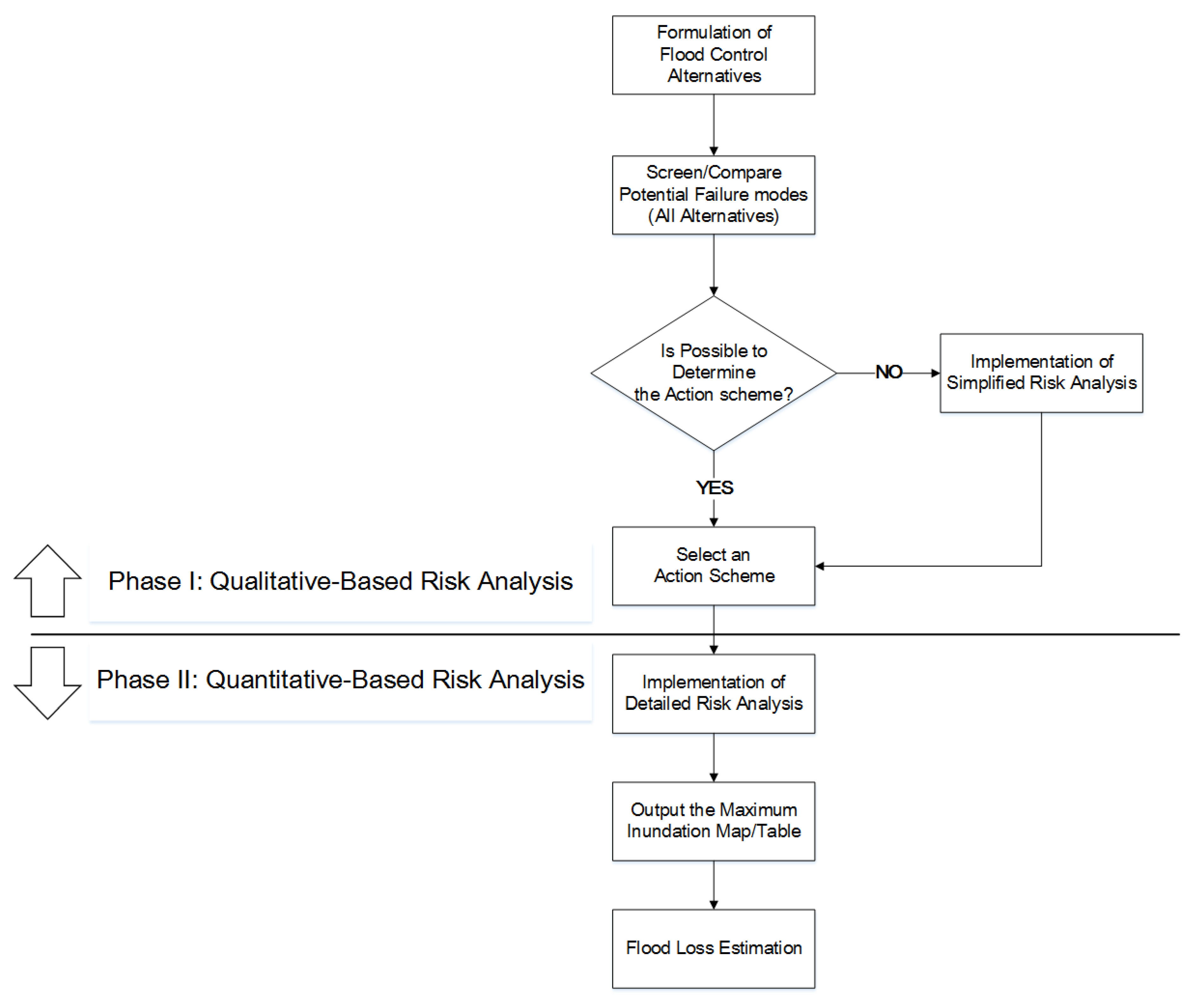
In this study, we proposed a two-phase risk-based analysis scheme and Chiang-Yuan drainage system was taken as a case study. The first phase is a qualitative screening process incorporating the principles of FMEA to identify all potential failure modes associated with candidate flood control measures [27]. The standard procedure for implementing FMEA includes: (1) developing a worksheet to identify and failure modes and effects; (2) giving each failure mode a probability ranking, a severity ranking and a detectability ranking, (3) multiply the three numbers for each failure mode, also known as the risk priority number (RPN), (4) prioritizing the failure modes. Scheme selection related flood control measures depends on the judgment of experts and screening results [6]. In the event that qualitative analysis is insufficient to derive a suitable solution, then simple risk analysis is used to quantify the inundation volume associated with each of the candidate solutions. All assumptions underlying risk analysis are based on the experience and expert knowledge of engineers. The second phase involves using numerical simulation to conduct quantitative evaluation of the selected engineering scheme. This analysis includes detailed risk analysis aiming at quantifying the spatial distribution of maximum inundation depth and the total potential losses associated with flood inundation under a variety of scenarios and hydrologic conditions as well as the failure of hydraulic facilities.

2.2. Simulation Tools

SOBEK developed by WL Delft Hydraulics [32] was selected as a simulation tool for the aforementioned detailed risk analysis, which is often used in flood inundation analysis studies [33,34,35,36,37]. This model is an integrated numerical modeling package based on one-dimensional (1D) St Venant equations [38]. It is widely used in Taiwan to deal with practical engineering projects where floodplain inundation plays an important role.

GIS-based modeling can be used to integrate flood inundation simulation models with loss estimation models [39]; however, we used GIS only as a component in the pre- and post-processing of spatial inundation data (input and output). We adopted this approach because inundation loss estimation in this study is limited to direct damage to agriculture land by flooding.

3. Overview of Study Area

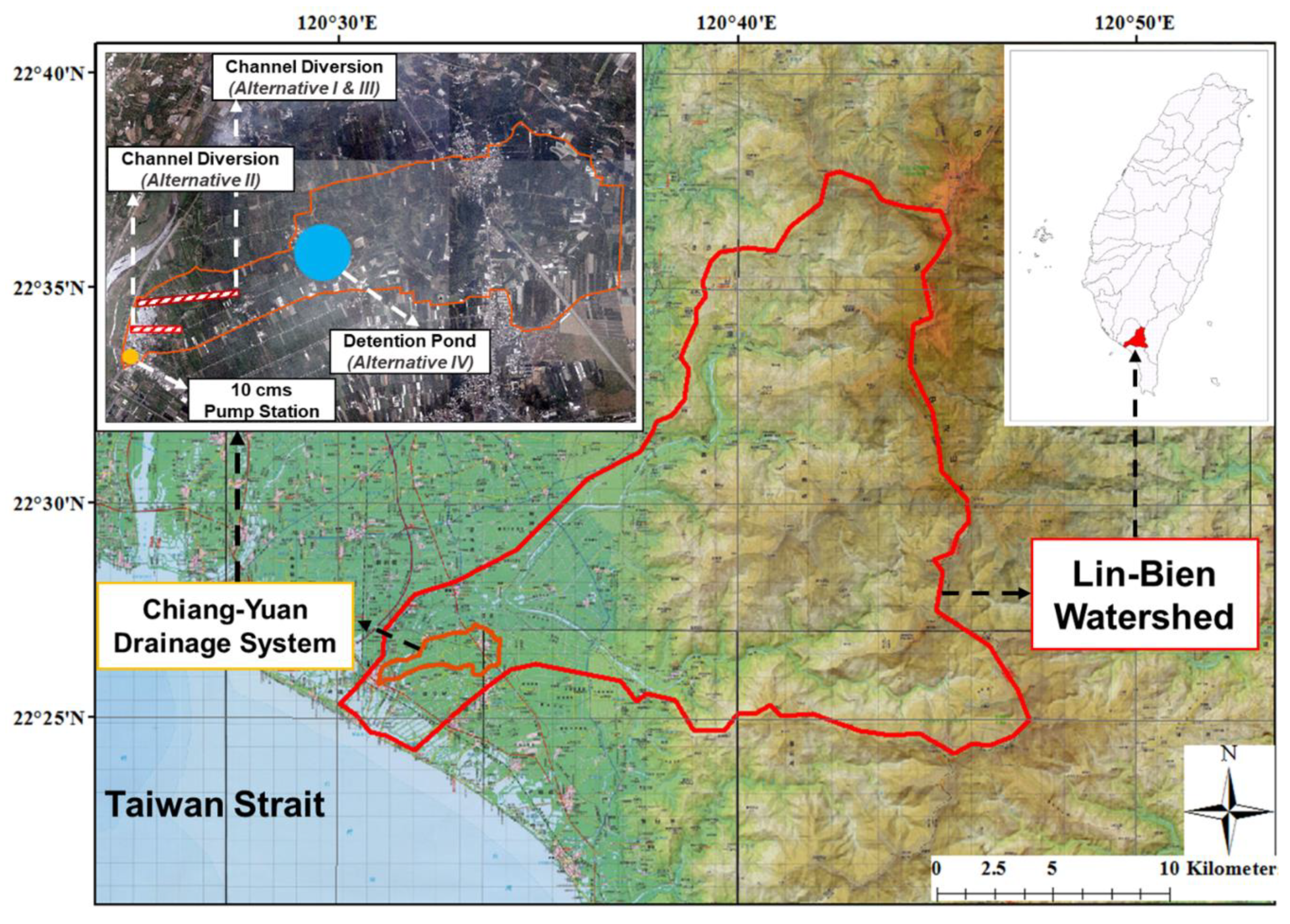
Lin-Bien River is located in central Pingtung, the southernmost county in western Taiwan (Figure 1). The total length of the river is 42 km and its catchment area is 336.30 km². Chiang-Yuan is a drainage system within the Lin-Bien catchment (marked in Figure 1), with a length of 9023 m and area of 6.93 km². The elevation ranges between 0 m and 27 m and 83.28% of the land elevation at Chiang-Yuan (highlands) is higher than the water stage at the downstream boundary of Lin-Bien River. This means that discharge from upstream can be driven by gravity. Most of the land in the Chiang-Yuan area is for agriculture and a small amount for aquaculture. Pingtung plain is agriculturally productive with a favorable tropical climate. The study region receives annual precipitation of 2100 mm approximately, most of which falls between May and October. The 100 year return period 24-h rainfall could reach 542 mm and 200 year 24-h rainfall could be 597 mm. The uneven distribution of rainfall leads to widespread flooding.

An increase in the number of extreme rainfall events due to climate change has brought the issue of regional inundation to the forefront. The WRA (Water Resource Agency, Ministry of Economy Affairs, Taiwan) in Taiwan has proposed a series of projects to deal with flooding issues in flood-prone areas [40,41]. The drainage system near the Lin-Bien catchment is one of the areas included in the project.

Lin-Bien River is located at the outlet of Chiang-Yuan drainage system. The pre-planning scenario conducted prior to the installation of flood control measures indicated that the channel water level could reach 3.1 m at the 10-year return period design discharge. Despite the fact that the main channel section from the downstream boundary to 1 km upstream has been augmented, the height of the natural embankment and the conveyance were insufficient to accommodate the inflow from upstream. The resulting overbank flow could incur considerable economic losses. Since most people live in the highland around the Chiang-Yuan drainage system, no casualty have occurred duo to flooding. Furthermore, the ground elevation of 16.72% area in the downstream near the drainage channel is substantially lower than the sea level. This means that water from Lin-Bien River could intrude into the inner drainage system and inner flow cannot drain by gravity while the sea level is high. Despite the installation of two pumps (capacity of 0.3 m³/s) at the downstream outlet of the drainage system, downstream villages are still exposed to a higher risk of inundation.

The risk of flooding is due to the insufficient conveyance of the main channel and the influence of backwater effects from Lin-Bien river’s stage as the external downstream boundary condition of this system. These factors hinder the release of floodwaters via the downstream section of Chiang-Yuan drainage system. The installation of hydraulic facilities will be necessary to mitigate the risk of flooding and associated economic losses.

4. Application and Results

4.1. Phase 1: Qualitative-Based Risk Analysis

4.1.1. Flood Control Options

The government has initially formulated five flood control options to increase the conveyance of the main drainage channel of Chiang-Yuan Drainage system [41]. All of the proposed flood control measures are structural in nature, as outlined in

Table 1. The detailed information of the five flood control alternatives.

Alternative Number	Description of Flood-Damage-Reduction Measures	Total Cost (Billion NTD)
I	a. A 1.500 km length open channel diverted at the 1.930 km upstream from the downstream boundary	0.32
	b. Embankment heightened between upstream 3.860 km to 1.930 km from the downstream boundary
II	a. A 0.630 km length open channel diverted at the 1.035 km upstream from the downstream boundary	0.28
	b. Embankment heightened between upstream 2.653 km to 1.035 km from the downstream boundary
III	a. A 1.500 km length box culvert diverted at the 1.930 km upstream from the downstream boundary	0.4
	b. Embankment heightened between upstream 4.795 km to 1.935 km from the downstream boundary
IV	a. A 4.00 m deep detention pond (50 ha) was set up at upstream of Chiang Yuan Drainage System	0.5
V	a. Embankment heightened between downstream boundary to its 2.6 km upstream	0.35
	b. A 4 km Water collocation system was set behind the embankment
	c. A 9 cms pump was set at near the downstream boundary

.

The selection of flood control measures was based on the need to limit flow discharge into the lowland area. Figure 1 shows the locations in which the various control measures would be installed. The objective behind options I, II and III was to divert discharge from the highlands in the upstream channel to the Lin-Bien River. Options I and II are the open-channel diversions respectively located at points 1.930 km and 1.035 km from the downstream outlet. It was planned that the height of the channel embankment would be increased from the diversion to the point of 3.860 km or 2.653 km upstream. Option III would divert the upstream discharge into the same location as Option I; however, a box culvert would be used. It was planned that the height of the channel embankment would be increased over a longer distance, extending from the diversion to a point 4.795 km upstream. The length of the diversion would be 1.500 km for options I and III but only 0.630 km for option II. The objective behind option IV would be to collect discharge from a point further upstream through the installation of a detention pond. The location of the detention pond was not specified; however, it would be in an area close to the intersection between the highland and lowland areas.

Unlike the first four options, option V was not meant to divert flow to other channels or stored it in the highland area upstream. The height of the channel embankment would be increased between the downstream boundary and a point 2.6 km upstream with the aim of preventing overflow in lowland areas. A 4 km water collocation system behind the embankment and a downstream pump (with capacity of 9 cm/s) would also be used for the removal of discharge from the drainage channel in lowland areas. Nonetheless, in the specific locations for these systems were never specified.

4.1.2. Scheme Selection

Figure 2 presents the procedure for selecting a remedial action plan. This procedure begins with the screening of all possible risk factors associated with the five remediation options. Overbank flow adjacent to the main drainage channel and diversion channel was identified as the most pressing threat associated with options I and II. Option III threatened additional overbank flow at the inlet of the box culvert. Option IV raised the greatest concern associated with a large area of land requisition by government. The fact that option IV would also imposed the highest capital expenditure eliminated it from consideration.

It was observed that the functionality of the pump station is critical to the safety of low-lying areas. If the pump station were submerged by channel discharge, the lowland damage caused by inundation could be severe. Thus, a pump system (10 m³/s) was installed at the outlet of Chiang-Yuan Drainage system prior to commencing the project at Lin-Bien River. Thus, option V, which relies heavily on additional pump stations, was not considered a viable candidate for the remedial project in this study.

Qualitative analysis is insufficient to judge the viability of Options I, II and III; therefore, we implemented a simplified risk analysis model. Three scenarios were formulated to assess the flooding risks associated with the three options. Despite the fact that the existing drainage channel and proposed open-channel or box culvert diversion (in options I, II and III) would provide sufficient capacity to avoid flooding in the foreseeable future; however, there remains a strong possibility that the conveyance would be compromised by sedimentation. Thus, we assumed three scenarios in which the highland channel maintained: (1) full conveyance, (2) two-thirds capacity and (3) half capacity. The three scenarios differ in the ability of the system to deal with highland discharge but impose the same requirement that lowland discharge be drawn off using the 10 cm/s pump at the downstream outlet of the system.

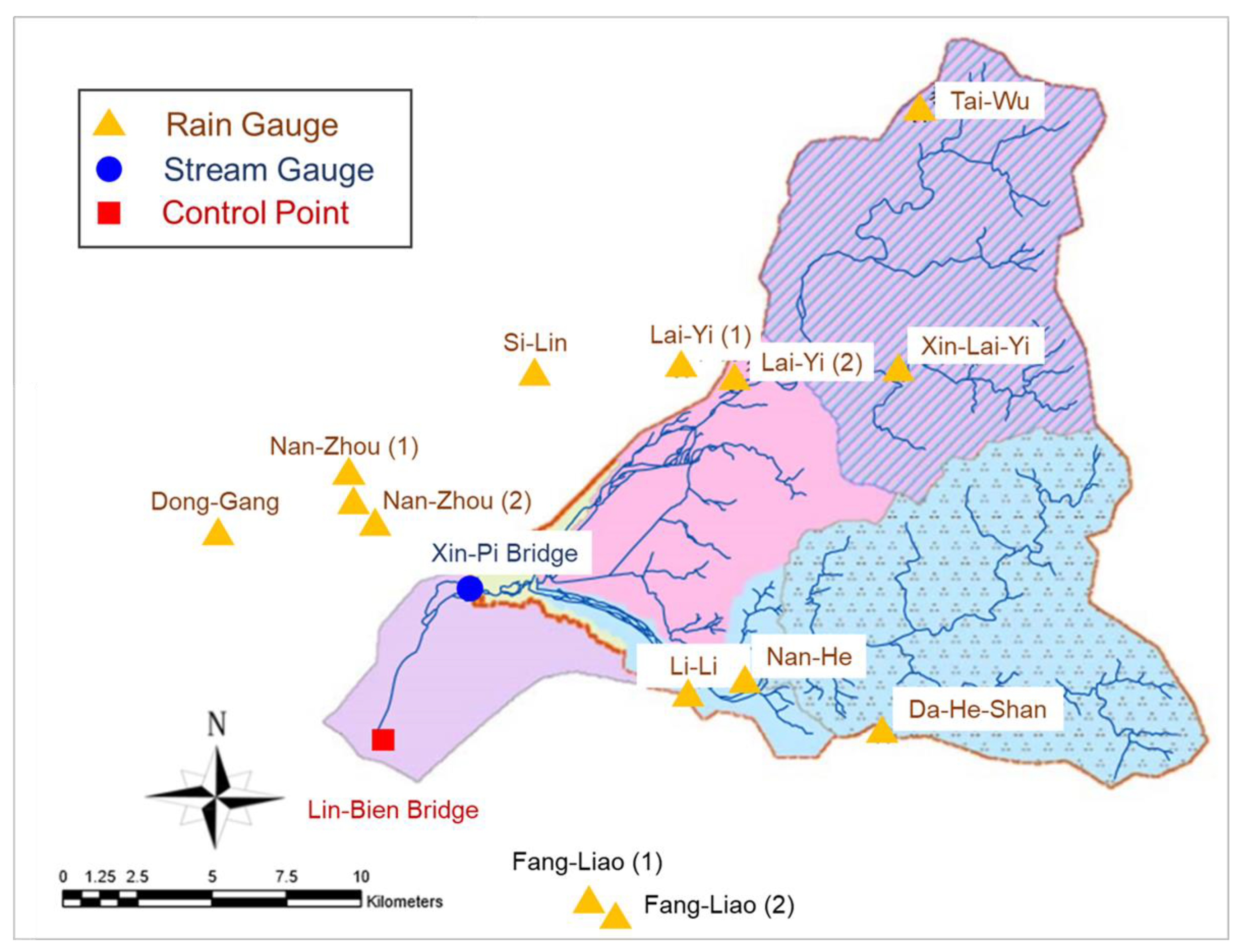
According to a government report [41], no rain gauges are located precisely within the Chiang-Yuan Drainage system. Therefore, we used annual precipitation data from fourteen rain gauges in the vicinity of the simulation area to derive the maximum two-day precipitation in the study area using the isohyetal method. The relatively flat topography in the study area and the strong influence of the external boundary on drainage efficiency means that the concentration time is larger than urban or mountainous areas. For this reason, we opted not to use storm patterns in the calculation of rainfall intensity. We uses the 48-hour design from the planning report of Lin-Bien watershed, in which the Lin-Bien Bridge was used as a control point [40]. The location of the hydrologic gauges and control point are indicated in Figure 3.

In this study, we estimated the inundation volume and depth based on the highland and lowland discharge of the 10-yr design standard. The discharge associated with the various recurrence intervals was derived using the triangular hydrograph method based on maximum two-day precipitation data [41]. The proportion made up by highland areas (83.28%) and lowland areas (16.72%) was used to determine the distribution of the total discharge. As shown in

Table 2. The peak flow information in Chiang-Yuan Drainage system.

Return Period (year)	1.1	2	5	10	25	50	100
Peak Flow (m3/s)	19.36	41.85	59.44	68.97	78.76	84.97	90.13
Highland Discharge (m3/s)	16.12	34.85	49.5	57.44	65.59	70.76	75.06
Lowland Discharge (m3/s)	3.24	7	9.94	11.53	13.17	14.21	15.07

, we selected a 10-year design flood as the design standard, as follows: highland areas (57.44 cm/s) and lowland areas (11.53 cm/s). The analysis process was further simplified by disregarding factors pertaining to land use in neighboring areas. The discharge was set as follows: highland areas (60 cm/s) and lowland areas (10 cm/s).

Table 3. The overall inundation results of simplified risk analysis.

(a) Full flood carrying capacity for alternative I, II and III
Return period (year)	1.1	2	5	10	25	50	100
Highland overflow (over 60 cms)
Time (hour)	-	-	-	-	4.09	7.3	9.63
Volume (m3)	-	-	-	-	41,181	141,441	261,077
Lowland overflow (over 10 cms)
Time (hour)	-	-	-	6.38	11.55	14.21	16.15
Volume (m3)	-	-	-	17,580	65,876	107,635	147,360
The overall results for the inundation analysis
Volume (m3)	-	-	-	17,580	65,876	107,635	147,360
Drainage Time (hour)	-	-	-	0.49	2.97	6.92	11.35
Inundation Depth (m)	-	-	-	0.03	0.19	0.43	0.71
(b) Two-thirds flood carrying capacity for alternative I, II and III
Return period (year)	1.1	2	5	10	25	50	100
Highland overflow (over 60 cms)
Time (hour)	-	-	9.21	14.57	18.73	20.87	22.42
Volume (m3)	-	-	157,576	457,422	862,686	1,155,487	1,414,927
Lowland overflow (over 10 cms)
Time (hour)	-	-	-	6.38	11.55	14.21	16.15
Volume (m3)	-	-	-	17,580	65,876	107,635	147,360
The overall results for the inundation analysis
Volume (m3)	-	-	157,576	475,002	928,562	1,263,122	1,562,287
Drainage Time (hour)			4.38	13.19	25.79	35.09	43.40
Inundation Depth (m)	-	-	0.27	0.82	1.61	2.19	2.71
(c) Half flood carrying capacity for alternative I, II and III
Return period (year)	1.1	2	5	10	25	50	100
Highland overflow (over 60 cms)
Time (hour)	-	6.68	18.91	22.93	26.05	27.65	28.82
Volume (m3)	-	58,377	663,798	1,132,464	1,668,613	2,028,804	2,337,174
Lowland overflow (over 10 cms)
Time (hour)	-	-	-	6.38	11.55	14.21	16.15
Volume (m3)	-	-	-	17,580	65,876	107,635	147,360
The overall results for the inundation analysis
Volume (m3)	-	58,377	663,798	1,150,044	1,734,489	2,136,439	2,484,534
Drainage Time (hour)	-	1.62	18.44	31.95	48.18	59.35	69.01
Inundation Depth (m)	-	0.10	1.15	1.99	3.01	3.70	4.30

lists the results of simplified risk analysis in terms of inundation depth and total inundation volume under the three scenarios. Using a 10-year design flood for full flood conveyance, we can see that the highland areas did not undergo inundation, due to the fact that the discharge (57.44 cm/s) was less than the design standard (60 cm/s). The highland inundation occurred when the discharge quantity attained the 25-year design flood. On the contrary, the inundation occurred at the lowland where the discharge (11.53 cm/s) exceeds the design standard of 10 cm/s. In this scenario, the drainage time was shown to be 0.49 h. The definition of drainage time is defined as the time required for a fully functional 10 cm/s pump to draw out sufficient discharge to prevent the occurrence of flooding in highland as well as lowland areas. Inundation depth was derived by dividing the total inundation volume by the overall drainage area (6.93 km²), resulting in a depth of 0.03 m. The estimation of total inundation volume, drainage time and inundation depth generally involves the quantity of water from both highland and lowland areas. For years of higher hydrologic activity (25 years/50 years/100 years), the results are as follows: total inundation volume (65,876 ${\mathrm{m}}^3$/107,635 ${\mathrm{m}}^3$/147,360 ${\mathrm{m}}^3$), drainage time (2.97 h/6.92 h/11.35 h) and inundation depth (0.19 m/0.43 m/0.71 m).

Table 3b,c respectively list the results of simplified risk analysis for the scenarios involving 66% conveyance and 50% conveyance. In highland areas, flooding could occur in 5-year and 2-year recurrence intervals under these two scenarios. The decrease in highland conveyance resulted in an additional 457,422 ${\mathrm{m}}^3$ or 1,132,464 ${\mathrm{m}}^3$ of inundation volume and 0.79 m or 1.96 m of inundation depth. For years of higher hydrologic activity (25 years/50 years/100 years), the inundation depth was as follows: 66% capacity (1.42 m/1.76 m/2.00 m) and 50% capacity (2.82 m/3.27 m/3.59 m). These results clearly illustrate the severe consequence of a decrease in conveyance due to the accumulation of sediment in drainage channels. Considering the difficulties involved in dredging a box culvert, (compared to an open channel), we surmise that option III would face a higher risk of inundation (compared to options I and II), thereby eliminating it as an option for the remedial action plan.

Simplified risk analysis confirmed option II as the optimal remedial action plan, due to its ability to divert highland discharge, low implementation cost and ease of dredging. The fact that the diversion path of option II is shorter than that of option I would also be helpful in preventing the expansion of inundation area from overbank flow. This first step is a time-saving procedure which avoid too much following complete numerical analysis.

4.2. Phase 2: Quantitative-Based Risk Analysis

4.2.1. Flood Inundation Model Setup

With the first step examination, we selected option II (open-channel diversion) to reduce the risk of flooding in the Chiang-Yuan Drainage system. The model was originally developed using SOBEK by the Water Resource Planning Institute (WRPI), Water Resources Agency. The SOBEK Chiang-Yuan model used in this study was previously calibrated and validated by [42]. Two models were established: the original drainage system and the system renovated using the remedial action plan. The grid size in the simulation module was set at 20 m × 20 m. In each simulation, we derived the maximum inundation depth over a period of 48 h (simulated) using the 1D Flow Module and 2D Overland Flow Module in SOBEK. GIS was also used to produce inundation maps by reclassifying the size of the flood area based on differences in maximum inundation depth.

4.2.2. Simulation Scenarios

The simulation scenarios were divided into those of diverse hydrologic conditions and those associated with failure modes. The diverse hydrologic situations simulated the study area without the proposed upgrades were adopted as a control.

Table 4. The information of simulation Scenarios.

Without Project Scenarios	Diverse Hydrologic (With Project) Scenarios	Failure Mode Scenarios
2-year return period of 48 h precipitation	2-year return period of 48 h precipitation	10-year of high external water stage
5-year return period of 48 h precipitation	5-year return period of 48 h precipitation	10-year of low external water stage
10-year return period of 48 h precipitation	10-year return period of 48 h precipitation	25-year of high external water stage
25-year return period of 48 h precipitation	25-year return period of 48 h precipitation	25-year of low external water stage
50-year return period of 48 h precipitation	50-year return period of 48 h precipitation	10-year short duration rainfall
100-year return period of 48 h precipitation	100-year return period of 48 h precipitation	25-year short duration rainfall
-	-	10-year high Manning’s value
-	-	10-year half channel transect
-	-	10-year pump station failure
-	-	25-year pump station failure

lists the information related to the scenarios using in the simulations. All simulations were based on the aforementioned SOBEK models using a maximum two-day precipitation series as input data for diverse hydrologic conditions.

The hydraulic model SOBEK is employed to simulate failure mode scenarios for further analysis. As shown in Table 4, we assumed that the water level under the 48-hour event was 1.38 m higher or 0.68 m lower than the tidal stage of Lin-Bien River, based on previous reports [41]. The former value was used to determine the severity of flooding; that is, river bank overtopping event can cause difficulties for internal draining. The latter value was used to examine whether the low external boundary could lead to higher hydraulic gradient and flow velocity which may cause the channel scour at the downstream section.

In a summary of several recent studies, Westra et al., 2014 [43] concluded that extreme rainfall at sub-daily time scales intensifies more rapidly than does rainfall measured at daily time scales, which increases the magnitude and frequency of flash floods. Based on the results of two-day precipitation under various recurrence intervals, we first selected 3 h as the rainfall duration by deriving the coefficients of Intensity-Duration-Frequency (IDF) curve using the objective function [41]. In case of rainfall scenarios of short durations, three-hour precipitation with the alternating block method is used to decide the rainfall pattern.

To take into account situations in which the channel path is congested with sediment, we increased Manning’s n coefficient to a factor or ten times the normal condition and reduced the cross sectional area of the diversion to half its original size. The first adjustment is meant to simulate situations in which the conveyance is significantly reduced, whereas the latter value is meant to simulate situations involving the collapse of the diversion.

We also took into account the possibility of pump station failure, such that the channel is overwhelmed. We adopted 10-year and 25-year design precipitation as the background hydrologic setting for the simulation of all failure mode scenarios, except those involving decreased conveyance, for which we used only 10-year precipitation values.

4.2.3. Diverse Hydrologic Scenarios

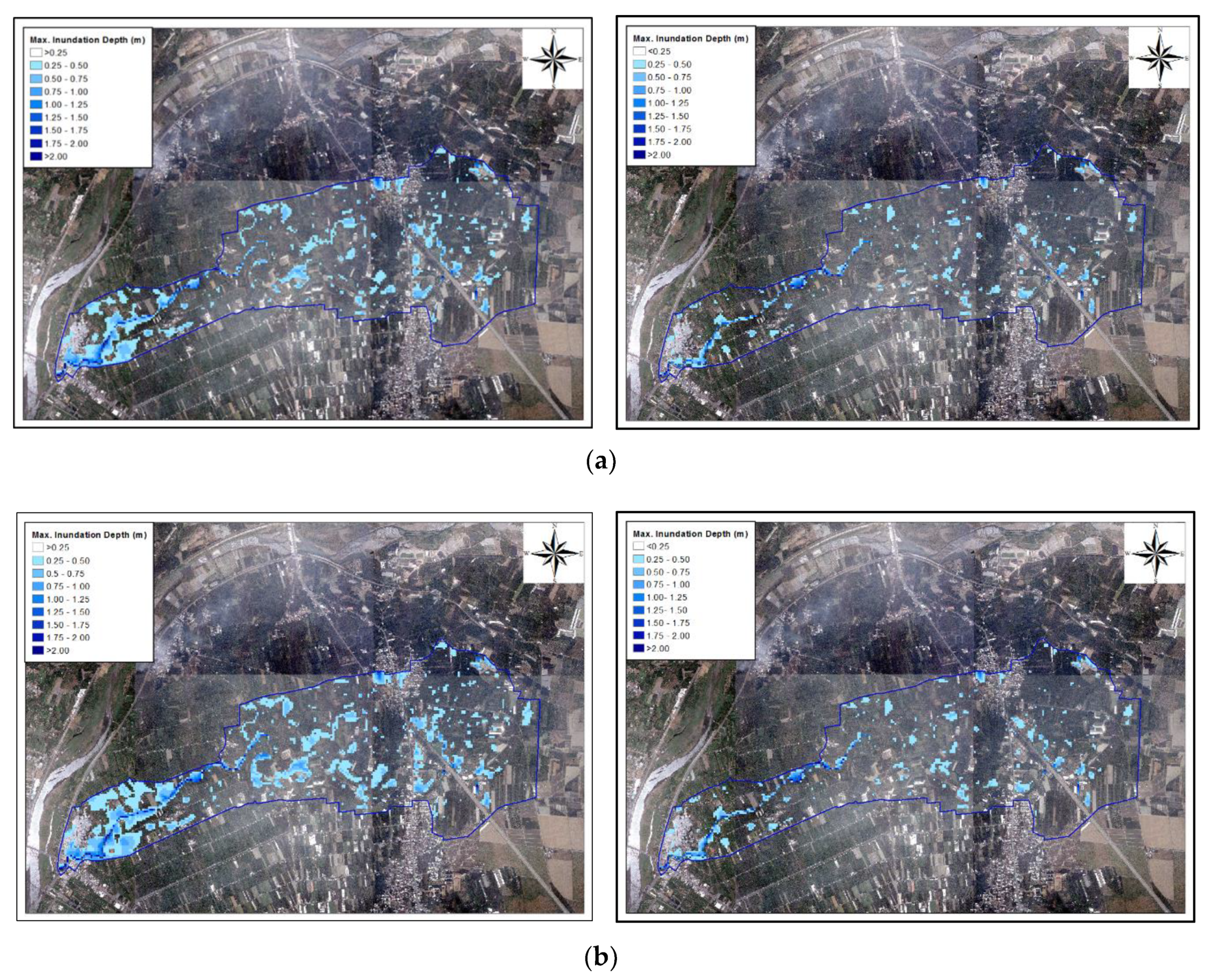
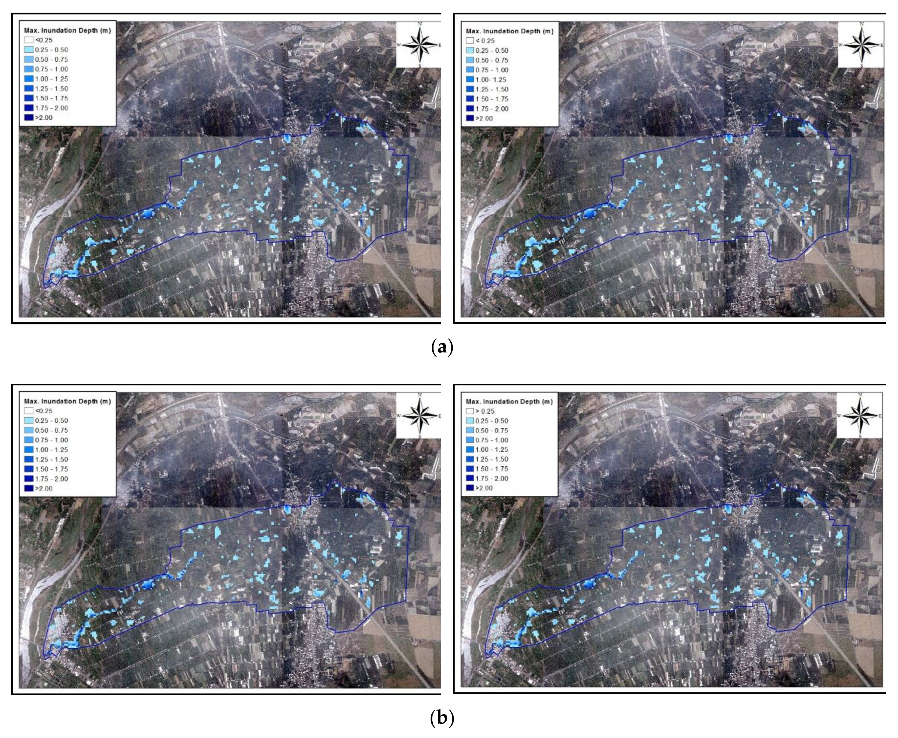
One of our objectives in this case study was to verify the efficacy of the proposed flood control measures. We therefore focused on a comparison of results obtained with and without the implementation of the remedial action plan. Figure 4 presents maps showing the spatial distribution of inundation area based on differences in the maximum inundation depth in the Chiang-Yuan Drainage system. Figure 4a,b clearly show that the depth of inundation was less in scenarios in which the remedial action plan was implemented. The inundation area was also reduced in highland as well as lowland areas. Before the application of flood control plan, the maximum inundation depth and inundation area for both highland and lowland have been observed to increase. However, following the adoption of the remedial action plan, the inundation results in highland and lowland areas presented similar range and scale regardless of recurrence interval. Furthermore, the inundation area of less than 1.00 m in lowland areas diminished significantly under all recurrence intervals. Moreover, most of the inundation in lowland areas was in the vicinity of the raised embankments and the pump station. This is a clear indication of the usefulness of the diversion in mediating overbank flow.

The maximum inundation depth corresponding to different design precipitation conditions is worth further examined for better understanding of the improvement on flood inundation. Thus, we summarize inundation area based on the diverse intervals of maximum inundation depth for the without and with project scenarios in

Table 5. The inundation area of different hydrologic scenarios for with project and without project (The difference of maximum inundation depth is derived by subtracting without project scenario from with project scenario for all return periods).

Maximum Inundation Depth (m)	Without Project 2-year (ha)	With Project 2-year (ha)	2-year Difference (ha)	Without Project 5-year (ha)	With Project 5-year (ha)	5-year Difference (ha)
<0.25 m	534.44	565.32	−30.88	520.64	561.68	−41.04
0.25 m–0.50 m	47.88	24.88	23	56.2	27.16	29.04
0.50 m–0.75 m	11.52	5.44	6.08	15.36	6.44	8.92
0.75 m–1.00 m	3.2	1.4	1.8	4.36	1.48	2.88
1.00 m–1.25 m	1.32	1.44	−0.12	1.44	1.4	0.04
1.25 m–1.50 m	1.04	1.56	−0.52	1.04	1.52	−0.48
1.50 m–1.75 m	0.88	0.52	0.36	0.96	0.6	0.36
1.75 m–2.00 m	0.52	0.24	0.28	0.72	0.52	0.2
>2.00 m	0.36	0.36	0	0.44	0.36	0.08
Maximum Inundation depth (m)	Without project 10-year (ha)	With project 10-year (ha)	10-year Difference (ha)	Without project 25-year (ha)	With project 25-year (ha)	25-year Difference (ha)
<0.25 m	509.96	559.12	−49.16	496.08	556.92	−60.84
0.25 m–0.50 m	62.52	29.16	33.36	70.28	30.72	39.56
0.50 m–0.75 m	18.16	6.72	11.44	22.2	7.04	15.16
0.75 m–1.00 m	5	1.64	3.36	6.16	1.92	4.24
1.00 m–1.25 m	2.08	1.4	0.68	2.68	1.28	1.4
1.25 m–1.50 m	1.04	1.52	−0.48	1.12	1.56	−0.44
1.50 m–1.75 m	0.96	0.72	0.24	0.76	0.8	−0.04
1.75 m–2.00 m	0.88	0.48	0.4	1.16	0.52	0.64
>2.00 m	0.56	0.4	0.16	0.72	0.4	0.32
Maximum Inundation depth (m)	Without project 50-year (ha)	With project 50-year (ha)	50-year Difference (ha)	Without project 100-year (ha)	With project 100-year (ha)	100-year Difference (ha)
<0.25 m	488.32	555.04	−66.72	480.56	553.6	−73.04
0.25 m–0.50 m	74.16	32.16	42	78.6	33.44	45.16
0.50 m–0.75 m	24.8	7.4	17.4	26.2	7.24	18.96
0.75 m–1.00 m	6.92	1.96	4.96	8.44	2.24	6.2
1.00 m–1.25 m	2.8	1.2	1.6	2.88	1.08	1.8
1.25 m–1.50 m	1.32	1.6	−0.28	1.52	1.72	−0.2
1.50 m–1.75 m	0.96	0.88	0.08	1	0.92	0.08
1.75 m–2.00 m	1	0.52	0.48	0.92	0.48	0.44
>2.00 m	0.88	0.4	0.48	1.04	0.44	0.6

, which also indicates the difference of inundation area for different intervals of maximum inundation depth between without and with project scenarios. In Table 5, for each interval of maximum inundation depth, the positive difference referred to the decrement of inundation area whereas the negative difference referred to the increment of inundation area.

Our results show that when the water depth was smaller than 0.25 m and that between 1.25 m and 1.50 m, the implementation of remedial action plan increased the inundation area, regardless of the recurrence intervals. The inundation area (<0.25 m and 1.25 m–1.50 m) under all recurrence intervals (2-year/5-year/10-year/25-year/50-year/100-year/) increased by 30.88 ha/41.04 ha/49.16 ha/60.84 ha/66.72 ha/73.04 ha (<0.25 m) and 0.52 ha/0.48 ha/0.48 ha/0.44 ha/0.28 ha/0.20 ha. For the 2-year and 25-year recurrence intervals, this increase also occurred when the maximum inundation depth was between 1.00 m to 1.25 m/1.50 m to 1.75 m. The inundation area increased by 0.12 ha/0.04 ha. However, after implementing the suggested remedial action plan, the inundation area decreased significantly at other depths. The results demonstrate the effectiveness of the remedial action plan in reducing the area affected by deep inundation.

We further obtained a rough estimation of the inundation volume. Our results show that the decrease in inundation volume became more pronounced with longer recurrence intervals. The decreased volumes (measured in million ${\mathrm{m}}^3$) were as follows: 0.1040 (2-year), 0.1438 (5-year), 0.1805 (10-year), 0.2322 (25-year), 0.2613 (50-year), 0.2911 (100-year). The total inundation volume increased with the length of the recurrence interval; however, the average inundation volume was decreased by more than 0.2 million cubic meters, due to the fact that the recurrence interval exceeded the normal design standard (10-year).

4.2.4. Failure Mode Scenarios

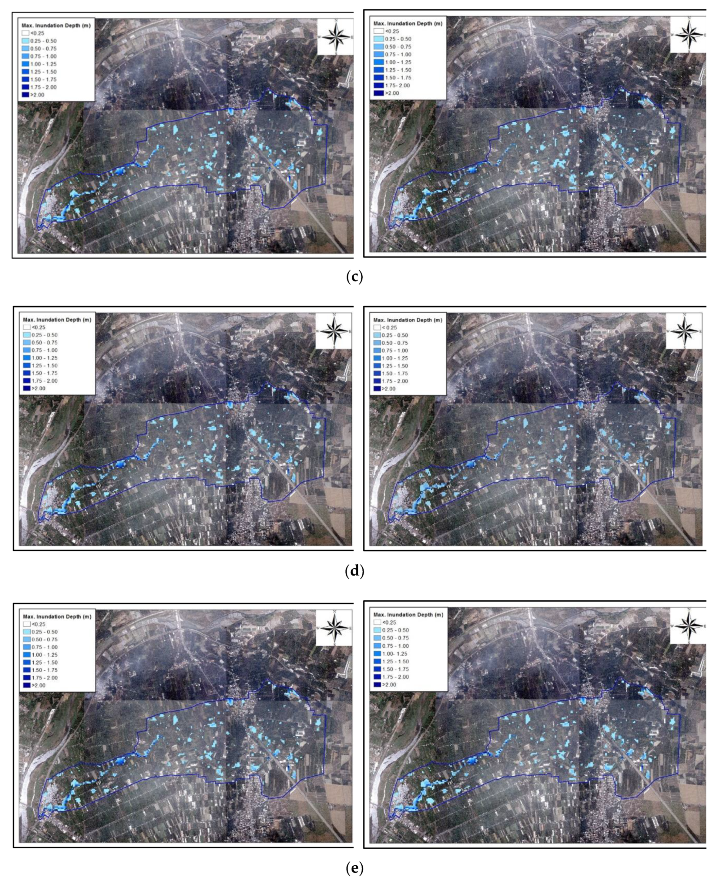
We also sought to elucidate how the inundation area would be affected in the case that flood control measures fail to maintain full functionality. Figure 5 presents the maximum inundation depth under all failure mode scenarios, including with the scenarios of high downstream water stage, the scenarios of low water stage in the external boundary, scenarios involving short duration precipitation and scenarios involving pump station failure with 25-year recurrence intervals. We also looked at two scenarios involving decreased conveyance (high Manning’s n value or half cross-section for diversion) under 25-year recurrence interval. Figure 5 presents maps showing the locations where the amount of inundation area actually increased after the implementation of the remedial action plans. This arrangement is because the inundation increment is not quantitatively significant for failure mode cases. The red mark indicates the difference in inundation areas of various depths between scenarios with fully functioning remedial action plans and cases of failure.

Table 6. The mitigation results of inundation volume for failure mode scenarios (The difference of maximum inundation depth is derived by subtracting with project scenarios from failure mode scenarios for all return periods).

Maximum Inundation Depth(m)	10-year High External Water Level (ha)	Difference with with Project Condition (ha)	25-year High External Water Level (ha)	Difference with with Project Condition (ha)	10-year Short Duration Rainfall (ha)	Difference with with Project Condition (ha)	10-year High Value of Manning’s n (ha)	Difference with with Project Condition (ha)	10-year Pump Station Failure (ha)	Difference with with Project Condition (ha)
<0.25 m	556.24	−2.88	553.08	−3.84	559.84	0.72	554.12	−5	557.24	−1.88
0.25 m–0.50 m	30.64	1.48	33.24	2.52	30.16	1	32.4	3.24	30.12	0.96
0.50 m–0.75 m	7.44	0.72	7.6	0.56	6.24	−0.48	7.92	1.2	7.32	0.6
0.75 m–1.00 m	1.92	0.28	2.24	0.32	1.52	−0.12	2.04	0.4	1.84	0.2
1.00 m–1.25 m	1.2	−0.2	1.2	−0.08	1.32	−0.08	1.24	−0.16	1.28	−0.12
1.25 m–1.50 m	1.8	0.28	1.72	0.16	1.28	−0.24	1.56	0.04	1.6	0.08
1.50 m–1.75 m	0.92	0.2	1.08	0.28	0.44	−0.28	0.96	0.24	0.88	0.16
1.75 m–2.00 m	0.52	0.04	0.44	−0.08	0.28	−0.2	0.44	−0.04	0.48	0
>2.00 m	0.48	0.08	0.56	0.16	0.08	−0.32	0.48	0.08	0.4	0
Maximum Inundation Depth (m)	10-year low external water level (ha)	Difference with with project condition (ha)	25-year low external water level (ha)	Difference with with project condition (ha)	25-year short duration rainfall (ha)	Difference with with project condition (ha)	10-year half transectarea (ha)	Difference with with project condition (ha)	25-year pump station failure (ha)	Difference with with project condition (ha)
<0.25 m	559.28	0.16	557.16	0.24	555.32	−1.6	555.56	−3.56	554.52	−2.4
0.25 m–0.50 m	29.08	−0.08	30.56	−0.16	33.56	2.84	31.4	2.24	32.48	1.76
0.50 m–0.75 m	6.68	−0.04	7.04	0	6.92	−0.12	7.76	1.04	7.28	0.24
0.75 m–1.00 m	1.64	0	1.84	−0.08	1.6	-0.32	1.84	0.2	2.24	0.32
1.00 m–1.25 m	1.36	−0.04	1.32	0.04	1.44	0.16	1.24	−0.16	1.16	−0.12
1.25 m–1.50 m	1.56	0.04	1.56	0	1.4	−0.16	1.6	0.08	1.6	0.04
1.50 m–1.75 m	0.68	−0.04	0.8	0	0.44	−0.36	0.88	0.16	0.96	0.16
1.75 m–2.00 m	0.48	0	0.48	−0.04	0.4	−0.12	0.44	−0.04	0.48	−0.04
>2.00 m	0.4	0	0.4	0	0.08	−0.32	0.44	0.04	0.44	0.04

shows the areas affected by inundation of various depths for each failure mode. It also shows the difference in inundation area of various depths between in scenarios with fully functioning remedial action plans and cases of failure. The positive values refer to an increase in the inundation area, whereas the negative values refer to a decrease in the inundation area.

Scenarios based on the external boundary with water levels of 10-year and 25-year recurrence intervals, revealed that the inundation area of any depth could increase, except in the case where the depth is below 0.25 m or between 1.00 m to 1.25 m. We observed a larger increase in the inundation area of 0.25 m–0.75 m deep, compared to any other depth. The inundation area at a depth of 0.25 m–0.50 m and 0.50 m to 0.75 m increased by 1.48 ha and 0.72 ha (10-year) and 2.52 ha and 0.56 ha (25-year). This is a clear indication that the high external downstream boundary would increase the inundation area in lowland areas, including upstream lowland areas and the original drainage channel in the vicinity of the diversion.

Conversely, the inundation area decreased for different depth intervals as the low external boundary has increased the drainage efficiency. As shown in Table 6, using 10-year recurrence intervals, the inundation area of various depths (0.25 m–0.50 m/0.50 m–0.75 m/1.00 m–1.25 m/1.50 m–1.75 m) decreased by 0.08 ha/0.04 ha/0.04 ha/0.04 ha. Using 25-year recurrence intervals, the inundation area of various depths (0.25 m–0.50 m/0.50 m–0.75 m/1.00 m–1.25 m/1.50 m–1.75 m) decreased by 0.16 ha/0.08 ha/0.04 ha. Nonetheless, it still can be found the increment of inundation area when the maximum inundation depth is less than 0.25 m or between 1.00 m to 1.50 m for both recurrence intervals. The inundation area of various depths (<0.25 m/1.25 m–1.50 m) using 10-year recurrence intervals increased by 0.16 ha/0.04 ha. The inundation area of various depths (<0.25 m/1.00 m–1.25 m) increased by 0.24 ha/0.04 ha using 25-year recurrence intervals. The low external boundary appears not to have a notable influence on local draining. Figure 5b also shows that the difference in the inundation area does not vary significant in the scenarios where remedial action plans were implemented by the external water levels were low.

The scenario involving precipitation over a short duration is a special case. As shown in Figure 5c, a smaller area was affected by inundation (of any depth) when remedial action plans were implemented, due to a reduction in the volume of water. Nonetheless, we observed an increase in the inundation area in upstream highland areas. As shown in Table 6, compared with the scenarios without engineering projects, the inundation area decreased when the depth of the inundation was less than 0.50 m for a 10-year recurrence interval. We observed an increase of 0.72 ha/1.00 in the inundation area of various depths (<0.25 m/0.25 m–0.50 m) for the 10-year recurrence interval. By contrast, we observed a decrease in the inundation area of between 0.25 m to 0.50 m and 1.00 m and 1.25 m for the 25-year recurrence interval. We observed an increase of 2.84 ha/0.16 ha in the inundation area of various depths (0.25 m–0.50 m/1.00 m–1.25 m) for 10-year recurrence interval. We infer from this that the maximum inundation depth would likely increase with higher downstream water level in the external boundary.

Our results for scenarios involving precipitation for short durations (extreme rainfall on the sub-daily scale) does not actually reflect reality. In SOBEK, the position of rain gauges is stationary despite the fact that extreme rainfall at the sub-daily scale involves spatial as well as temporal uncertainty. We therefore believe that estimates of the inundation area should be conservative with a focus on failure mode scenarios. This would make it easier to elucidate the magnitude and frequency of flood occurrences.

Figure 5d presents two scenarios involving a decrease in the capacity of the diversions under the 10-year recurrence interval. As shown in Table 6, we observed the most pronounced increase in the inundation area at depths of 0.25 m to 1.00 m and appears as the depth between 1.25 m to 1.75 m or over 2.00 m. The inundation area of various depths (0.25 m–0.50 m/0.50 m–0.75 m/0.75 m–1.00 m/1.25 m–1.50 m/1.50 m–1.75 m/>2 m) increased by 3.24 ha/1.20 ha/0.40 ha/0.04 ha/0.24 ha/0.08 ha for the scenario using a high Manning’s n value. The inundation area increased by 2.24 ha/1.04 ha/0.20 ha/0.08 ha/0.16 ha/0.04 ha in the scenario using the half transect area. Figure 5d shows an increase in the inundation area upstream and downstream from the original drainage channel, rather than at the diversion. Implementing a higher Manning’s n value has a more pronounced effect than halving the flood conveyance in terms of increasing the inundation area. Nonetheless, decreasing of flood capacity should be seriously identified in the actual circumstances.

Pump station failure did not influence the inundation area as strongly as a decrease in conveyance. The inundation area of various depths (0.25 m–0.50 m/0.50 m–0.75 m/0.75 m–1.25 m/1.25 m–1.50 m/1.50 m–1.75 m/>2.00 m) increased by 0.96 ha/0.60 ha/0.20 ha/0.08 ha/0.16 ha/0.00 ha for the 10-year recurrence interval and by 1.76 ha/0.24 ha/0.32 ha/0.04 ha/0.16 ha/0.04 ha for the 25-year recurrence interval. Most importantly, we found the increment of inundation area was smaller than the scenario of decreasing of flood carry capacity in spatial which centered more on the vicinity of the confluence of original drainage channel and diversion as indicated in Figure 5e. From this, we can infer that a decrease in the conveyance of a diversion should has spatial similarity with pump station failure for a certain extent in considering the increment of inundation area.

4.2.5. Flood Loss Estimation

Estimating flood/inundation losses is an essential component in risk-oriented flood design, risk mapping and formulating financial appraisals in the reinsurance sector. Simple models, such as stage-damage curves, are widely used to estimate flood/inundation loss. Flood/inundation loss models require data sufficient to derive multi-factorial loss models to ensure validity [29]. Flood damage can be broadly classified as tangible and intangible. Tangible flood damage that can be expressed in monetary terms can be divided into direct and indirect damage, which can be further subdivided into primary and secondary damages [44,45]. Direct tangible flood damage is caused by direct contact with floodwater. In this study, most of the land in the study area is agricultural. We therefore assumed that the entire simulation space is agricultural in nature, such that losses are restricted to primary tangible damage.

This study illustrates the relationship between inundation depth on the Pingtung Plain and the reduction in agricultural yield per hectare (ha), based on historical data [46]. The reduction in agricultural yield associated with inundations of various depth (0.25 m–0.50 m/0.50 m–0.75 m/0.75 m–1.00 m/1.00 m–1.25 m/1.25 m–1.50 m/>1.50 m) were 17.0%/32.5%/47.5%/67.5%/90.0%/100.0%, respectively. We also observed a correlation between the reduction in agricultural yield and crop production period, inundation depth, inundation duration, flood turbidity and the depth of sediment accumulation. We estimated the loss of agriculture product due to inundation at 0.2 million ($ NTD) per hectare (ha).

Table 7. The results of Inundation loss for with and without project scenarios.

Return Period (year)	Inundation Loss of without Project Scenarios (Million $NTD)
	Without Project Loss	With Project Loss	Difference between With & Without Project
2	3.4	2.03	1.37
5	4.13	2.24	1.89
10	4.73	2.37	2.36
25	5.51	2.48	3.03
50	5.97	2.57	3.4
100	6.43	2.64	3.79

lists the monetary losses due to inundation in scenarios with and without the implementation of remedial action plans. The positive difference of inundation loss between without and with project scenarios refers to the decrement of economic loss and vice versa, after adopting the remedial action plan. We found that when the remedial action plans was implemented, monetary losses due to inundation increased when the inundation depth was between 1.00 m and 1.50 m, regardless of the recurrence interval. Clearly, the proposed remedial action plan can be beneficial in reducing economic losses. The monetary losses due to inundation (2-year/5-year/10-year/25-year/50-year/100-year) were 1.37 million/1.89 million/2.36 million/3.03 million/3.40 million/3.79 million NT dollars. Our results appear to be persuasive, particularly in light of the fact that the losses increased with the increasing recurrence interval.

Table 8. The results of Inundation loss for failure mode scenarios.

Failure Mode Scenarios	Total Inundation Loss of System Failure	Increase of Inundation Loss Due to System Failure
10-year high external water level	2.58	0.21
25-year high external water level	2.72	0.24
10-year low external water level	2.36	-0.01
25-year low external water level	2.47	-0.02
10-year short duration rainfall	2.14	-0.22
25-year short duration rainfall	2.37	-0.11
10-year high value of Manningll n	2.63	0.27
10-year half transect area	2.55	0.19
10-year pump station failure	2.49	0.12
25-year pump station failure	2.61	0.13

lists the economic losses due to inundation in scenarios involving the implementation of remedial action plans and where those plans failed. It is not surprising that the scenarios involving rainfall of short duration incur lower monetary losses due to less volume of flood during this short time. The scenarios of low water level in external boundary also showed the mitigation of inundation loss value(s) which could attain 0.01 million and 0.02 million NT dollars for 10-year and 25-year recurrence intervals. The remaining scenarios (10-year high external water level/25-year high external water level/10-year high value of Manning’s n/10-year half transect area/10-year pump station failure/25-year pump station failure) resulted in monetary losses of 0.21 million/0.24 million/0.27 million/0.19 million/0.12 million/0.13 million NT dollars, due to inundation. Our results confirm that boundary effects have a pronounced effect than pump station failure on inundation volume and monetary losses. The increment of monetary loss value(s) for the decreasing flood conveyance scenarios may be caused by the channel siltation in actual circumstances.

5. Conclusions

In this study, we proposed a two-phase risk analysis scheme for flood management, using qualitative risk analysis in the first phase and quantitative risk analysis in the second phase. The screening/comparison procedure in the first phase employs failure mode and effects analysis (FMEA) for the selection of the optimal remedial action plan in terms of mitigating the risks of flood/inundation. In the event that the qualitative approach fails to identify the optimal remedial action plan, then simplified risk analysis is used to quantify the volume of inundation associated with the various candidate plans. In the second phase, numerical simulations based on the results of quantitative analysis are conducted. The proposed flood management scheme was employed to investigate the Chiang-Yuan Drainage system as a cases study in order to evaluate its effectiveness.

Options IV (Detention Pond) and V (Pump Station) were ruled out in the screening process of the first phase, due to social and environmental concerns as well as the inherent dangers associated with a reliance on pumping stations. We also conducted simulations involving three scenarios in which the highland channel was limited in conveyance (relative to the 10-year recurrence interval) due to sedimentation. Simplified risk analysis revealed option II as the best remedial action plan, in terms of capital outlay and the threat of silting in the drainage channel.

Simulation results revealed that the implementation of the remedial action plan (installing diversions and the raising of embankments) reduced the inundation area in the highland as well as lowland areas, regardless of the recurrence interval. These efforts were shown to reduce the inundation volume by more than 0.2 million cubic meters under the 10-year design scenario.

We also conducted failure mode scenarios to determine how the area would be affected by inundation in the event that flood control measures were unable to maintain full functionality. Scenarios involving high downstream water stages in the external boundary were shown to increase the inundation area in lowland areas, upstream regions of the lowland areas and the original drainage channel in the vicinity of the diversion. Conversely, the inundation area decreased as low water stages in the external boundary increased drainage efficiency. The maximum flow velocity and water profiles in the diversion indicated that there would be no risk of channel erosion downstream or hydraulic jump. Scenarios involving precipitation of short duration are a special case. Though the inundation area of different maximum inundation depth was less than the scenarios with construction projects, the inundation area expanded at the upstream highland area. Unfortunately, the proposed scenario involving precipitation of short duration does not reflect reality due to the fact that the rain gauges in SOBEK are stationary. In the two scenarios involving a decrease in the conveyance of the channel(s), it revealed that the Manning’s n value has a more pronounced effect than the conveyance in terms of the inundation area. A failure of the pump station was shown to have less effect than the conveyance in terms of the inundation area. We can infer from this that the decreasing flood conveyance in diversion should has spatial similarity with pump station failure for a certain extent in considering the increment of inundation area.

Traditionally, the flood control practices are formulated with some design standard of protection, to remove the risk of flooding from events up to some return period, commonly the 1 in 100 year return period event. This study try to examine on how each intervention strategy will fail as a result of a more extreme event occurring or for other reasons. This study tries to realize the new concept of flood control which is called a design for failure [47]. Nonetheless, this analysis could be extended using advanced methodologies and tools. The proposed procedure is also applicable to more general engineering systems.

References

- Milly, P.C.; Dunne, K.A.; Vecchia, A.V. Global pattern of trends in streamflow and water availability in a changing climate. Nature 2005, 438, 347–350. [Google Scholar] [CrossRef] [PubMed]
- Tunstall, S.M.; Johnson, C.L.; Penning-Rowsell, E.C. Flood hazard management in England and Wales: From land drainage to flood risk management. In Proceedings of the World Congress on Natural Disaster Mitigation, New Delhi, India, 19–21 February 2004; pp. 19–21. [Google Scholar]
- Apel, H.; Thieken, A.H.; Merz, B.; Blöschl, G. A probabilistic modelling system for assessing flood risks. Nat. Hazards 2006, 38, 79–100. [Google Scholar] [CrossRef]
- Thieken, A.; Merz, B.; Kreibich, H.; Apel, H. Methods for flood risk assessment: Concepts and challenges. In Proceedings of the International Workshop on Flash Floods in Urban Areas, Muscat, Sultanate of Oman, 4–6 September 2006. [Google Scholar]
- Knight, F.H. Risk, Uncertainty, and Profit; Hart, Schaffner and Marx: New York, NY, USA, 1921. [Google Scholar]
- USACE. Guidelines for Risk and Uncertainty Analysis in Water Resources Planning Volume 1–Principles—With Technical Appendices; US Army Corps of Engineers, Water Resources Support Center, Institute for Water Resources: Washington, DC, USA, 1992. [Google Scholar]
- Haimes, Y.Y. Risk Modeling, Assessment, and Management; John Wiley & Sons: New York, NY, USA, 2015. [Google Scholar]
- UNISDR. Global Assessment Report on Disaster Risk Reduction 2013; UNISDR: Geneva, Switzerland, 2013. Available online: http://go.nature.com/LBJ4xL (accessed on 18 December 2018).
- Mileti, D. Disasters by Design: A Reassessment of Natural Hazards in the United States; Joseph Henry Press: Washington, DC, USA, 1999. [Google Scholar]
- Merz, B.; Kreibich, H.; Thieken, A.; Schmidtke, R. Estimation uncertainty of direct monetary flood damage to buildings. Nat. Hazards Earth Syst. Sci. 2004, 4, 153–163. [Google Scholar] [CrossRef] [Green Version]
- Klijn, F.; Kreibich, H.; De Moel, H.; Penning-Rowsell, E. Adaptive flood risk management planning based on a comprehensive flood risk conceptualisation. Mitig. Adapt. Strat. Glob. Chang. 2015, 20, 845–864. [Google Scholar] [CrossRef]
- USACE. Risk-Based Analysis of Flood Damage Reduction Studies; EM1110-2-1619; U.S. Army Corps of Engineers: Washington, DC, USA, 1996. [Google Scholar]
- USACE. Risk-Based Analysis for Evaluation of Hydrology/Hydraulics, Geotechnical Stability, and Economics in Flood Damage Reduction Studies; ER1105-2-101; U.S. Army Corps of Engineers: Washington, DC, USA, 1996. [Google Scholar]
- Hydrologic Engineering Center. HEC-FDA Flood Damage Reduction Analysis, User’s Manual, version 1.0, CPD-72; U.S. Army Corps of Engineers, Hydrologic Engineering Center: Davis, CA, USA, 1998. [Google Scholar]
- Meyer, V.; Scheuer, S.; Haase, D. A multicriteria approach for flood risk mapping exemplified at the Mulde river, Germany. Nat. Hazards 2009, 48, 17–39. [Google Scholar] [CrossRef]
- De Moel, H.; Aerts, J.C.J.H. Effect of uncertainty in land use, damage models and inundation depth on flood damage estimates. Nat. Hazards 2011, 58, 407–425. [Google Scholar] [CrossRef]
- Messner, F.; Meyer, V. Flood damage, vulnerability and risk perception–challenges for flood damage research. In Flood Risk Management: Hazards, Vulnerability and Mitigation Measures; Springer: Dordrecht, The Netherlands, 2006; pp. 149–167. [Google Scholar]
- USACE. Expected Annual Flood Damage Computation User’s Manual; U.S. Army Corps of Engineers: Washington, DC, USA, 1989; Available online: http://www.hec.usace. army.mil/publications/ComputerProgramDocumentation/CPD-30.pdf (accessed on 18 December 2018).
- Mays, L.W. Water Resources Engineering; John Wiley & Sons: New York, NY, USA, 2010. [Google Scholar]
- Apel, H.; Merz, B.; Thieken, A.H. Quantification of uncertainties in flood risk assessments. Int. J. River Basin Manag. 2008, 6, 149–162. [Google Scholar] [CrossRef] [Green Version]
- Merz, B.; Thieken, A.H. Flood risk curves and uncertainty bounds. Nat. Hazards 2009, 51, 437–458. [Google Scholar] [CrossRef] [Green Version]
- Apel, H.; Thieken, A.H.; Merz, B.; Blöschl, G. Flood risk assessment and associated uncertainty. Nat. Hazards Earth Syst. Sci. 2004, 4, 295–308. [Google Scholar] [CrossRef] [Green Version]
- Hall, J.W.; Sayers, P.B.; Dawson, R.J. National-scale assessment of current and future flood risk in England and Wales. Nat. Hazards 2005, 36, 147–164. [Google Scholar] [CrossRef]
- RWS-DWW. Flood Risks and Safety in the Netherlands (Floris); DWW-2006-014, Ministerie van Verkeer en Waterstaat; Rijkswaterstaat, DWW: Delft, The Netherlands, 2005. [Google Scholar]
- Szewrański, S.; Chruściński, J.; Kazak, J.; Świąder, M.; Tokarczyk-Dorociak, K.; Żmuda, R. Pluvial Flood Risk Assessment Tool (PFRA) for Rainwater Management and Adaptation to Climate Change in Newly Urbanised Areas. Water 2018, 10, 386. [Google Scholar] [CrossRef]
- Jamali, B.; Löwe, R.; Bach, P.M.; Urich, C.; Arnbjerg-Nielsen, K.; Deletic, A. A rapid urban flood inundation and damage assessment model. J. Hydrol. 2018, 564, 1085–1098. [Google Scholar] [CrossRef]
- Dod, D. Military Standard: Procedures for Performing a Failure Mode Effects and Criticality Analysis; Department of Defense: Washington, DC, USA, 1980.
- FERC (Federal Energy Regulatory Commission). Dam Safety Performance Monitoring Program (DSPMP)/Potential Failure Modes Analysis (PFMA) Chapter 14 Dam Safety Performance Monitoring Program; Federal Energy Regulatory Commission: Washington, DC, USA, 2005. Available online: https://www.ferc.gov/industries/hydropower/safety/guidelines/enguide/chap14.pdf (accessed on 1 July 2015).
- USACE (U.S. Army Corps of Engineers). USACE Process for the National Flood Insurance Program (NFIP) Levee System Evaluation; EC 1110-2-6067; U.S. Army Corps of Engineers: Washington, DC, USA, 2010. [Google Scholar]
- Wahalathantri, B.L.; Lokuge, W.; Karunasena, W.; Setunge, S. Vulnerability of floodways under extreme flood events. Nat. Hazards Rev. 2015, 17, 04015012. [Google Scholar] [CrossRef]
- Thieken, A.H.; Olschewski, A.; Kreibich, H.; Kobsch, S.; Merz, B. Development and evaluation of FLEMOps—A new Flood Loss Estimation MOdel for the private sector. WIT Trans. Ecol. Environ. 2008, 118, 315–324. [Google Scholar]
- Hydraulics, D. SOBEK: User’s Manual; Delft Hydraulics: Delft, The Netherlands, 2017. [Google Scholar]
- Becker, B.; Burzel, A. Model Coupling with OpenMI Introduction of Basic Concepts. In Managing the Complexity of Critical Infrastructures; Studies in Systems, Decision and Control; Setola, R., Rosato, V., Kyriakides, E., Rome, E., Eds.; Springer: Chambridge, UK, 2016; Volume 90. [Google Scholar]
- Buchacz, A.; Baier, A.; Herbuś, K.; Ociepka, P.; Grabowski, Ł.; Sobek, M. Compression studies of multi-layered composite materials for the purpose of verifying composite panels model used in the renovation process of the freight wagon’s hull. Eksploat. Niezawodn. Maint. Reliab. 2018, 20, 137–146. [Google Scholar] [CrossRef]
- Cuddington, K.; Sobek-Swant, S.; Crosthwaite, J.C. Probability of emerald ash borer impact for Canadian cities and North America: A mechanistic model. Biol. Invasions 2018, 20, 2661. [Google Scholar] [CrossRef]
- Gu, X.W.; Yang, W.L.; Dong, G.T.; Dang, S.Z. Application of One-Dimensional Hydraulic Model for Flood Simulation in Yellow River Delta. Adv. Mater. Res. 2014, 955–959, 2969–2972. [Google Scholar] [CrossRef]
- Li, H.; Wei, S.; Cheng, C.; Liou, J.; Chen, Y.; Yeh, K. Applying Risk Analysis to the Disaster Impact of Extreme Typhoon Events Under Climate Change. J. Disaster Res. 2015, 10, 513–526. [Google Scholar] [CrossRef]
- Chow, V.T. Open Channel Hydraulics; McGraw-Hill: New York, NY, USA, 1959. [Google Scholar]
- Dutta, D.; Herath, S. GIS based flood loss estimation modeling in Japan. In Proceedings of the US-Japan 1st Workshop on Comparative Study on Urban Disaster Management, Port Island, Kobe, Japan, February 2001; pp. 151–161. [Google Scholar]
- WRA (Water Resources Agency). The Planning Report of Lin-Bien River Watershed-Tributary Drainage Planning; Water Resources Agency, Ministry of Economic Affairs: Taiwan, China, 2008. (In Chinese)
- WRA (Water Resources Agency). The Remediation of flood-Prone Area in Lin-Bien River Watershed-Tributary Drainage Planning; Water Resources Agency, Ministry of Economic Affairs: Taiwan, China, 2009. (In Chinese)
- WRPI (Water Resources Planning Institute). Second Upgrading Potential Inundation Maps of PingTung County; Water Resources Planning Institute, Water Resources Agency, Ministry of Economic Affairs: Taiwan, China, 2014. (In Chinese)
- Westra, S.; Fowler, H.J.; Evans, J.P.; Alexander, L.V.; Berg, P.; Johnson, F.; Kendon, E.J.; Lenderink, G.; Roberts, N.M. Future changes to the intensity and frequency of short-duration extreme rainfall. Rev. Geophys. 2014, 52, 522–555. [Google Scholar] [CrossRef] [Green Version]
- Smith, D.I. Flood damage estimation—A review of urban stage-damage curves and loss functions. Water SA 1994, 20, 231–238. [Google Scholar]
- Dutta, D.; Herath, S.; Musiake, K. A mathematical model for flood loss estimation. J. Hydrol. 2003, 277, 24–49. [Google Scholar] [CrossRef]
- WRA (Water Resources Agency). Chapter 7 of Irrigation and Drainage Engineering-Drainage Planning and Design; Water Resources Agency, Ministry of Economic Affairs: Taiwan, China, 1981. (In Chinese)
- Green, C.H.; Parker, D.J.; Penning-Rowsell, E.C. Designing for failure. Nat. Disasters Prot. Vulnerable Communities 1993, 6, 78–91. [Google Scholar]
Figure 1.
The general location for the study area and the flood control measures.
Figure 2.
Two-phase risk-based application procedure of this study.
Figure 3.
The location for the hydrologic gauges and control point at near Lin-Bien Watershed.
Figure 4.
The inundation map for the without project and diverse hydrologic (with project) scenarios. (a) Comparison of inundation results for the low return periods (Before and After for 10-year); (b) Comparison of inundation results for the high return periods (Before and After for 100-year).
Figure 5.
The inundation map for the failure mode scenarios (Red mark refers to the inundation difference between the with project scenario and the indicated failure mode scenario). (a) Comparison scenarios for with project and high external water stage (25-year with project; 25-year high external water stage); (b) Comparison scenarios for with project and low external water stage (25-year with project; 25-year low external water stage); (c) Comparison scenarios for with project and short duration precipitation (25-year with project; 25-year short duration precipitation); (d) Comparison scenarios for with project and decreasing flood carrying capacity (25-year with project; 25-year decreasing flood carrying capacity); (e) Comparison scenarios for with project and pump station failure (25-year with project; 25-year pump station failure).