Rainfall Infiltration Modeling: A Review
by
 , , , and
Renato Morbidelli
1,* ,
,
Corrado Corradini
1,
Carla Saltalippi
1,
Alessia Flammini
1,
Jacopo Dari
1 and
and
Rao S. Govindaraju
2 1
Department of Civil and Environmental Engineering, University of Perugia, via G. Duranti 93, 06125 Perugia, Italy
2
Lyles School of Civil Engineering, Purdue University, West Lafayette, IN 47907, USA
*
Author to whom correspondence should be addressed.
Water 2018, 10(12), 1873; https://doi.org/10.3390/w10121873
Submission received: 7 December 2018
/
Accepted: 13 December 2018
/
Published: 18 December 2018
(This article belongs to the Special Issue Rainfall Infiltration Modeling)
Abstract
:Infiltration of water into soil is a key process in various fields, including hydrology, hydraulic works, agriculture, and transport of pollutants. Depending upon rainfall and soil characteristics as well as from initial and very complex boundary conditions, an exhaustive understanding of infiltration and its mathematical representation can be challenging. During the last decades, significant research effort has been expended to enhance the seminal contributions of Green, Ampt, Horton, Philip, Brutsaert, Parlange and many other scientists. This review paper retraces some important milestones that led to the definition of basic mathematical models, both at the local and field scales. Some open problems, especially those involving the vertical and horizontal inhomogeneity of the soils, are explored. Finally, rainfall infiltration modeling over surfaces with significant slopes is also discussed.
1. Introduction
Brutsaert [1] offers a concise definition of infiltration as “the entry of water into the soil surface and its subsequent vertical motion through the soil profile”. Infiltration plays an important role in the partitioning of applied surface water into surface runoff and subsurface water—both of these components govern water supply for agriculture, transport of pollutants through the vadose zone, and recharge of aquifers [2]. The infiltration of rain and surface water is influenced by many factors, including soil depth and geomorphology, soil hydraulic properties, and rainfall or climatic properties [3]. Researchers have understood for ages that rainfall wets the soil and may produce runoff. Our understanding of the physics of the process and the dynamics of porous media hydraulics has come rather recently. Our ability to mathematically describe the response of a soil to rainfall and to understand the parameters that affect infiltration, has developed only in the last few decades.
The spatio-temporal evolution of infiltration rate under natural conditions cannot be currently deduced by direct measurements at all scales of interest in applied hydrology, and infiltration modeling with the aid of measurable quantities is of fundamental importance.
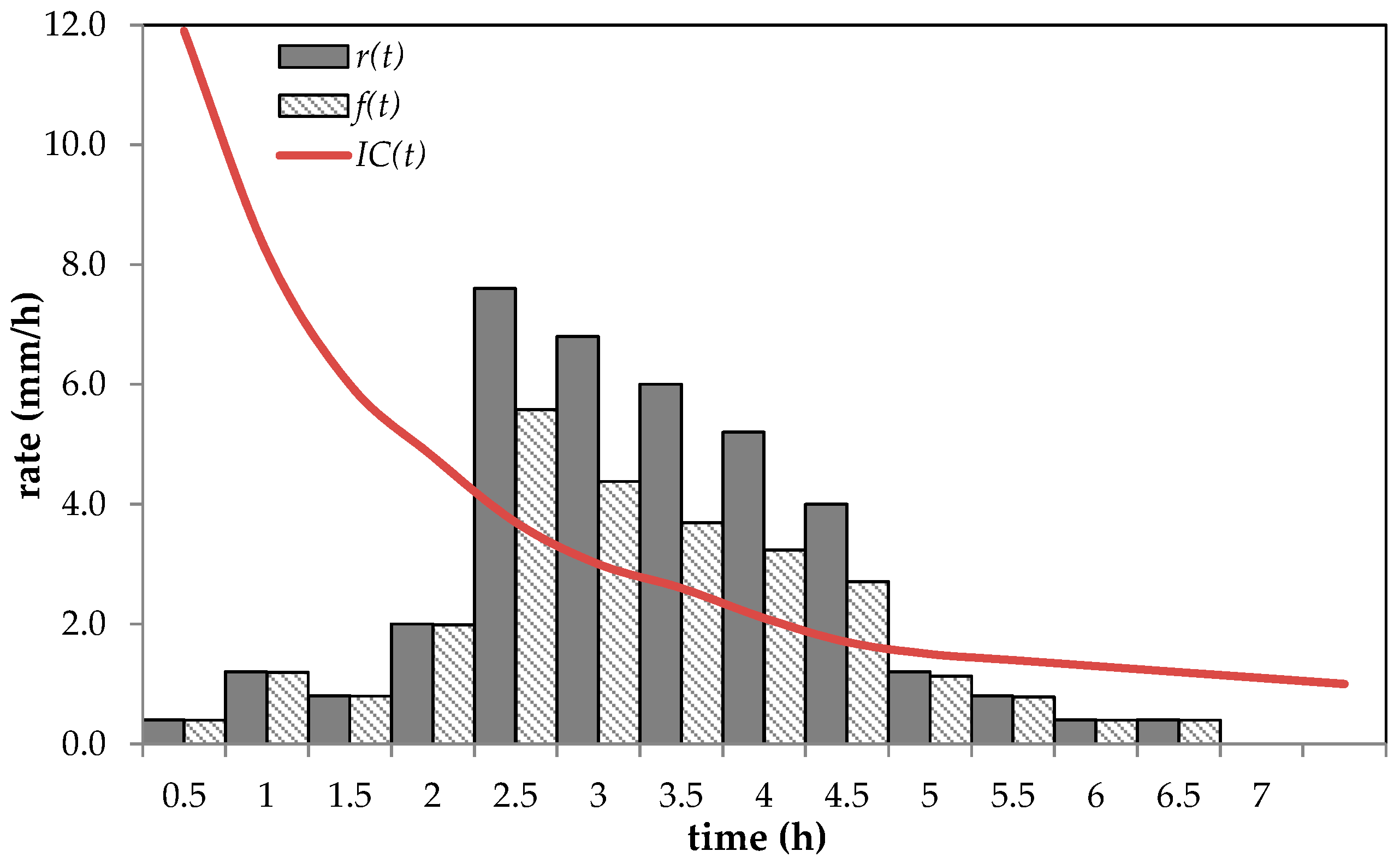
Even though the representation of the main natural processes in applied hydrology requires areal infiltration modeling for both flat and sloping surfaces, research activity has been limited to the development of local or point infiltration models for many years. A variety of local infiltration models for vertically homogeneous soils with constant initial soil water content and over horizontal surfaces has been proposed [4,5,6,7,8,9,10,11,12,13,14,15,16,17,18,19,20,21,22,23,24,25,26,27,28]. A milestone paper describing the process of infiltration from a ponded surface condition was published by Reference [4]. Successively, Reference [29] published his assessment of the role of infiltration in flood generation, defining “infiltration capacity” (IC) as a hyetograph separation rate that was generally applicable as a threshold for application to a rainfall intensity graph. A few years later, Reference [30] refined this concept by referring to it as an infiltration rate that declines exponentially during a storm, and then published a conceptual derivation of the exponential decay infiltration equation. On this basis, if the rainfall overcomes the IC, only a portion of it may infiltrate while the remaining quantity ponds over the surface or moves depending of the local slope. Therefore, the IC can be regarded as an important soil characteristic. As an example, Figure 1 shows several infiltration regimes when rainfall occurs over a soil surface. The line represents the IC(t) curve for a silty loam soil. The dark columns represent the rainfall rate, r(t), observed in the Umbria Region (Central Italy) during a generic frontal system. The dashed columns represent the simulated behavior of infiltration rate, f(t), during the rainfall event. With low values of rainfall intensities, the total amount of r(t) infiltrates through the soil surface and r(t) is equal to f(t). With high r(t) values only a part of the r(t) can infiltrate, while the difference r(t)−f(t) becomes runoff. As it can be observed, there exists no straightforward relationship between IC and runoff as the effective f(t) is a function of the specific rainfall intensity.
Natural soils are rarely vertically homogeneous. In hydrological simulations, the estimate of effective rainfall can be reasonably schematized by a two-layered vertical profile [31,32]. Soils representable by a sealing layer over the parent soil or a vertical profile with a more permeable upper layer are found frequently in nature. Some models for infiltration into stable crusted soils were developed under significant approximations by adapting the Green–Ampt model [33,34,35,36,37,38] or the two-stage infiltration equations proposed by Mein and Larson [39] for homogeneous soils. An efficient approach which represents transient infiltration into crusted soils was proposed by Reference [40], while Reference [41] formulated a model which describes upper-layer dynamics but in the limits of a ponded upper boundary. A more general semi-analytical/conceptual model for crusted soils was later formulated by Reference [42], and was extended by Reference [43] to represent infiltration and re-infiltration after a redistribution period under any rainfall pattern and for any two-layered soil where either layer may be more or less permeable than the other. For a much more permeable upper layer, and under more restrictive rainfall patterns, a simpler semi-empirical/conceptual model was presented by Reference [44]. Under conditions of surface saturation, a simple Green–Ampt-based model was proposed [45].
In applied hydrology, upscaling of point infiltration models to the field scale is required to estimate areal-average infiltration. This is a challenging task because of the natural spatial heterogeneity of hydraulic soil properties [46,47,48,49,50,51,52], and particularly of the soil saturated hydraulic conductivity [53,54] that may be assumed as a random field with a lognormal univariate probability distribution. The mathematical problem is not analytically tractable, whereas the use of accurate Monte Carlo (MC) simulation techniques imposes an enormous computational burden for routine applications. MC simulations were used, for instance, by References [55,56,57] to describe field-scale infiltration. MC simulations were also used by Reference [58] to corroborate a relation between areal average and variance of infiltration rate under a time-invariant rainfall rate; however, the averaging procedure was applied in space over a single realization and the behavior of the resulting errors was not specified. A variant to MC sampling for the representation of the random variability of a soil property is Latin Hypercube sampling [59] adopted by Reference [60] to develop a simple parameterized approach for areal-average infiltration.
Even though MC simulations, performed by many realizations of the random variable, are rather expensive in terms of computational effort for practical applications, they are useful as a tool to parameterize simple semi-empirical approaches or to serve as a benchmark for validating semi-analytical models. Along these lines, Reference [61] developed three versions of a semi-analytical/conceptual model for estimating the expected areal-average infiltration into vertically homogeneous soils under spatially uniform rainfall, but with random horizontal values of the saturated hydraulic conductivity (see also [62]). A shortcoming of this model is that the process of infiltration of overland flow running over pervious downstream areas (run-on process) is neglected. On the other hand, the importance of run-on was shown in a few investigations concerning the effects of horizontal variability of saturated hydraulic conductivity on Hortonian overland flow [57,63,64,65,66,67], but this process has generally been disregarded in hydrological models.
In addition to the heterogeneity of saturated hydraulic conductivity, rainfall is also characterized by spatial variability [68,69]. Some studies combining the random variability of these two quantities were performed by References [70,71,72]. The latter paper presented a semi-analytical model developed under less restrictive conditions, even though run-on was not incorporated, and was based upon the use of cumulative infiltration as the independent variable that was linked with an expected time. Subsequently, Reference [73] formulated a more complete mathematical model for the expected areal-average infiltration, which considers both the saturated hydraulic conductivity and rainfall rate as random variables, and then combines the aforementioned semi-analytical approach with a semi-empirical/conceptual component to represent the run-on process.
A model of the expected areal-average infiltration into a much more permeable upper layer of a two-layered soil was also proposed by Reference [74] considering only a spatial horizontal random field of the saturated hydraulic conductivity. It involves the solution of a set of algebraic equations obtained by upscaling simple local infiltration equations to the field scale. The areal-average infiltration for a vertically non-uniform soil characterized by a saturated hydraulic conductivity decreasing with depth according to a power law was derived by Reference [75] and upscaled to the field scale by the same semi-analytical technique used in previous papers [61,72].
Most of the above-mentioned models assumed zero or small surface slope that does not affect the infiltration process. However, in most real situations, infiltration occurs over surfaces characterized by different gradients [76,77] and the role of surface slope on infiltration is not clear. In fact, the results obtained by some theoretical and experimental investigations [78,79,80,81,82,83,84,85,86,87,88,89,90,91,92,93,94,95,96,97] lead to contrasting conclusions, suggesting that an improved understanding and modeling of infiltration on sloping surfaces is required.
Finally, when macropore flow plays a significant role in determining infiltration, amendments of the Darcy–Richards approach may be used, especially at the local scale [98,99].
The main intent of this review paper is to critically assess the complexities of the infiltration process and to provide guidance for developments related to open problems. This paper will provide classical approaches developed for rainfall events with continuous saturation at the soil surface, and a more general formulation suitable for any type of rainfall pattern for applications at the local (point) scale in homogeneous soils. Simple models for point infiltration into a two-layered soil with a more permeable upper layer and a more complex model for any two-layered soil type are presented. Semi-empirical and semi-analytical field-scale infiltration models are analyzed. Finally, problems linked to rainfall infiltration into surfaces with significant slopes are also discussed.
2. Basic Physical Models for Infiltration
By considering a horizontally homogeneous soil, water movement in the vertical direction is governed by one-dimensional soil water flow and continuity equations. The flow rate, q, per unit cross-sectional area is described by Darcy’s law, actually proposed by Reference [100], as:
where K is the hydraulic conductivity, ψ is the soil water matric capillary head, and z is the vertical soil depth assumed positive downward. The infiltration rate, q0, is given by Equation (1) applied at the soil surface.
In the absence of changes in the water density and soil porosity as well as of sinks and sources, the continuity equation is:
where θ is volumetric water content and t is time. The substitution of Equation (1) into Equation (2) leads to the well-known Richards equation:
where C1 = dθ/dψ and C2 = dK/dψ with a typical assumption that θ and K are unique functions of ψ thus neglecting hysteresis in these functions. The initial condition at time t = 0 for z ≥ 0 is ψ = ψi, and the upper boundary conditions at the soil surface, where z = 0, are:
where r is the rainfall rate, tp is the time to ponding, and tr is the duration of rainfall. Hereafter the subscripts i and s denote initial and saturation quantities, respectively, while 0 stands for quantities at the soil surface. The lower boundary conditions at a depth zb which is not reached by the wetting front is ψ(zb) = ψi for t > 0. The soil water hydraulic properties can be represented by the following parameterized forms [22]:
where and are used as scaling quantities, ψb is the air entry head, θr is the residual volumetric water content, c, λ, and d are empirical coefficients, and b = 3 and a = 2 according to Burdine’s method [101]. For particular values of the parameters, Equations (5a) and (5b) reduce to the well-known equations proposed by References [101,102]. For two-layered soils, two additional conditions are required at the interface between the two layers:
where hereafter the subscripts 1, 2, and c denote variables in the upper layer, in the lower layer, and at the interface, respectively, and Zc is the interface depth.
q0 = r, 0 < t ≤ tp; θ0 = θs, tp < t ≤ tr; q0 = 0, tr < t,
In particular cases, it can be useful to express Equation (3) in terms of θ obtaining:
where D(θ) is the soil water diffusivity equal to K(θ)(dψ(θ)/dθ).
3. Point Infiltration Modeling for Homogeneous Soils
Many local infiltration models for vertically homogeneous soils with constant initial soil water content and over horizontal surfaces are widely recognized in the scientific literature [4,5,8,9,10,11,17,18,20,22,23,26,28,29,30,103]. Furthermore, for isolated storms and when ponding is not achieved instantly, extended forms of the Philip model [45], the Green–Ampt model [104,105], and the Smith and Parlange model [106] have been widely used, whereas for arbitrary rainfall patterns, the model presented in [26] serves as a useful method. These four models, together with a widely adopted equation suggested by References [29,30], have been extensively used in applied hydrology and as building blocks in the development of infiltration approaches at the field scale.
3.1. Horton Empirical Equation
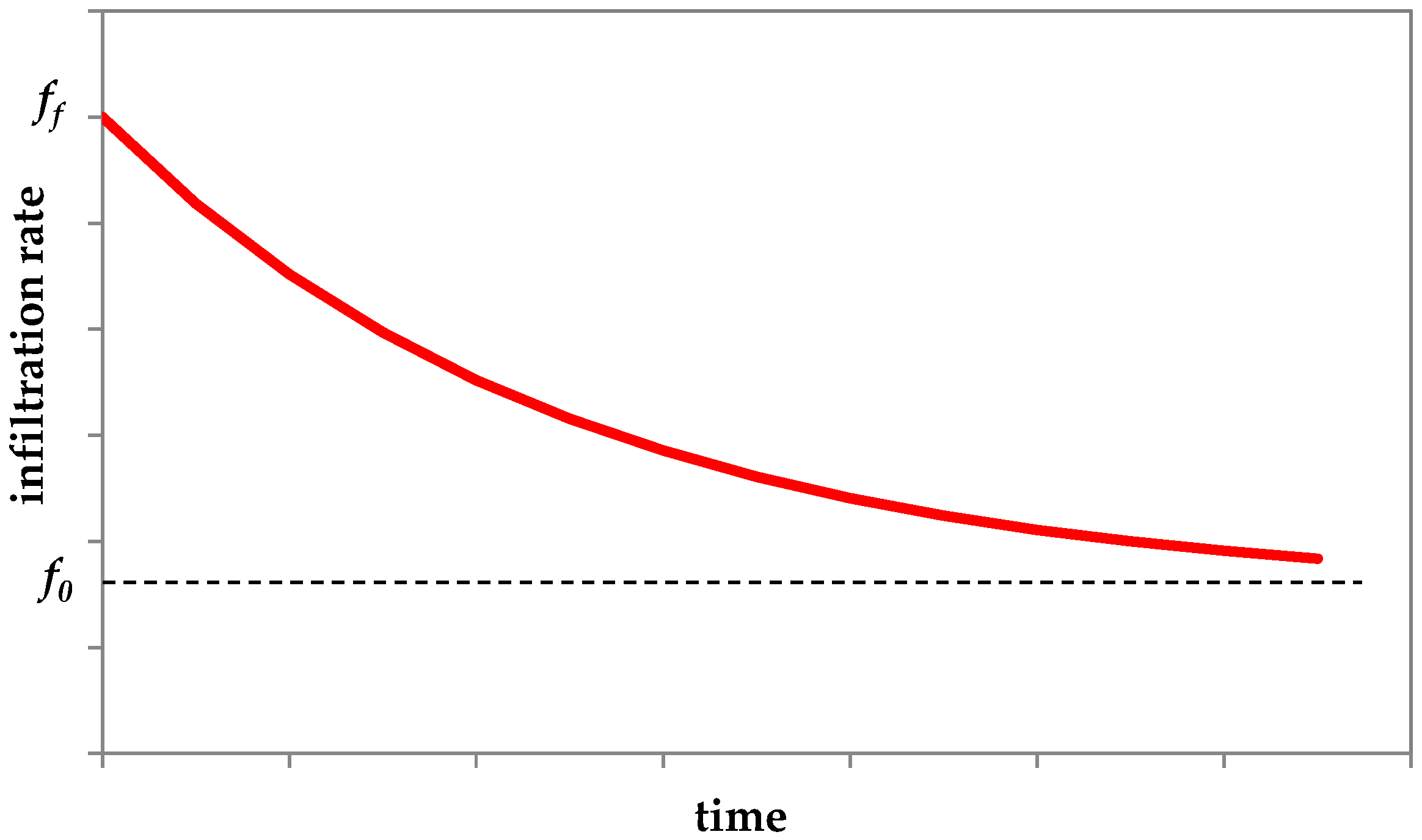
In the empirical equation proposed by References [29,30], the infiltration capacity, fc, exponentially decreases as follows (see also Figure 2):
where f0 and ff represent the initial and final values of fc, respectively, and α is the decay constant. When t→∞, ff can be considered equal to the saturated hydraulic conductivity of the soil. If K and D are independent of θ, References [107,108] demonstrated that Equation (8) can be obtained from Equation (7).
3.2. Philip Equation
A widely adopted analytical solution of the Richards equation was proposed by References [9,10,11,109] under the conditions of vertically homogeneous soil, constant initial moisture content, and saturated soil surface with immediate ponding. For early to intermediate times the semi-analytical solution for the infiltration capacity, based on a series expansion and truncation after the first two terms, is expressed as:
where S is the sorptivity, depending on soil properties and initial moisture content, and A is a quantity ranging from 0.38 Ks to 0.66 Ks. For t→∞, Equation (9) is replaced by fc = Ks. The integration of Equation (9) yields the cumulative infiltration:
Philip’s model was extended for applications to less restrictive conditions. For a constant rainfall rate r > Ks, surface saturation occurs at a time tp > 0 and, following [45], infiltration can be described through an equivalent time origin, t0, for potential infiltration after ponding as:
For unsteady rainfall under the condition of a continuously saturated surface for t > tp, the infiltration process can be represented adopting a similar procedure. Generally, S and A are derived from the calibration of hydrological models; however, S can also be approximated as [110]:
where ϕ is the soil porosity and ψav is the soil water matric capillary head at the wetting front.
3.3. Green–Ampt Model
This model represents infiltration into homogeneous soils under the conditions of continuously saturated soil surface and uniform initial soil moisture as:
where F the cumulative depth of infiltrated water. To express the infiltration as a function of time, this equation can be solved after the substitution fc = dF/dt. The resulting equation [45] is:
Equation (16) assumes immediate ponding and an infinite supply of water at the surface. Under more general conditions, with a constant rainfall rate r > Ks, that begins at the time t = 0, surface saturation is reached at a time tp > 0. For t ≤ tp, the infiltration rate q0 is equal to r and later to the infiltration capacity. Mein and Larson [104] formulated this process through Equation (15) as:
which leads to the determination of tp as:
Furthermore, for t > tp, Equation (16) becomes:
Equation (19) can be solved at each time, for example, by successive substitutions of F which is then substituted into Equation (15) to obtain the corresponding value of fc.
3.4. Parlange–Lisle–Braddock–Smith Model
A 3-parameter model obtained through an analytical integration of the Richards equation has been formulated by Reference [106] and can be expressed as:
where F′ = F − Kit is the cumulative dynamic infiltration rate, α is a parameter linked to the behavior of hydraulic conductivity and soil water diffusivity as functions of θ, and G is the integral capillary drive defined by:
Equation (20) includes as limiting forms [60] the Reference [17] equation (α = 1) and the Green–Ampt equation (α→0). It can be applied to determine tp and fc for any rainfall pattern, and for t > tp can be rewritten under the condition of surface saturation in a time dependent form as:
where Kd = Ks − Ki and F′p = F′(tp). The quantities F′p and tp are the values of F′ and t at ponding, respectively, at which Equation (20) with fc = r(tp) is first satisfied. The value of α usually ranges from 0.8 to 0.85 [3].
3.5. Corradini–Melone–Smith Semi-Analytical/Conceptual Model
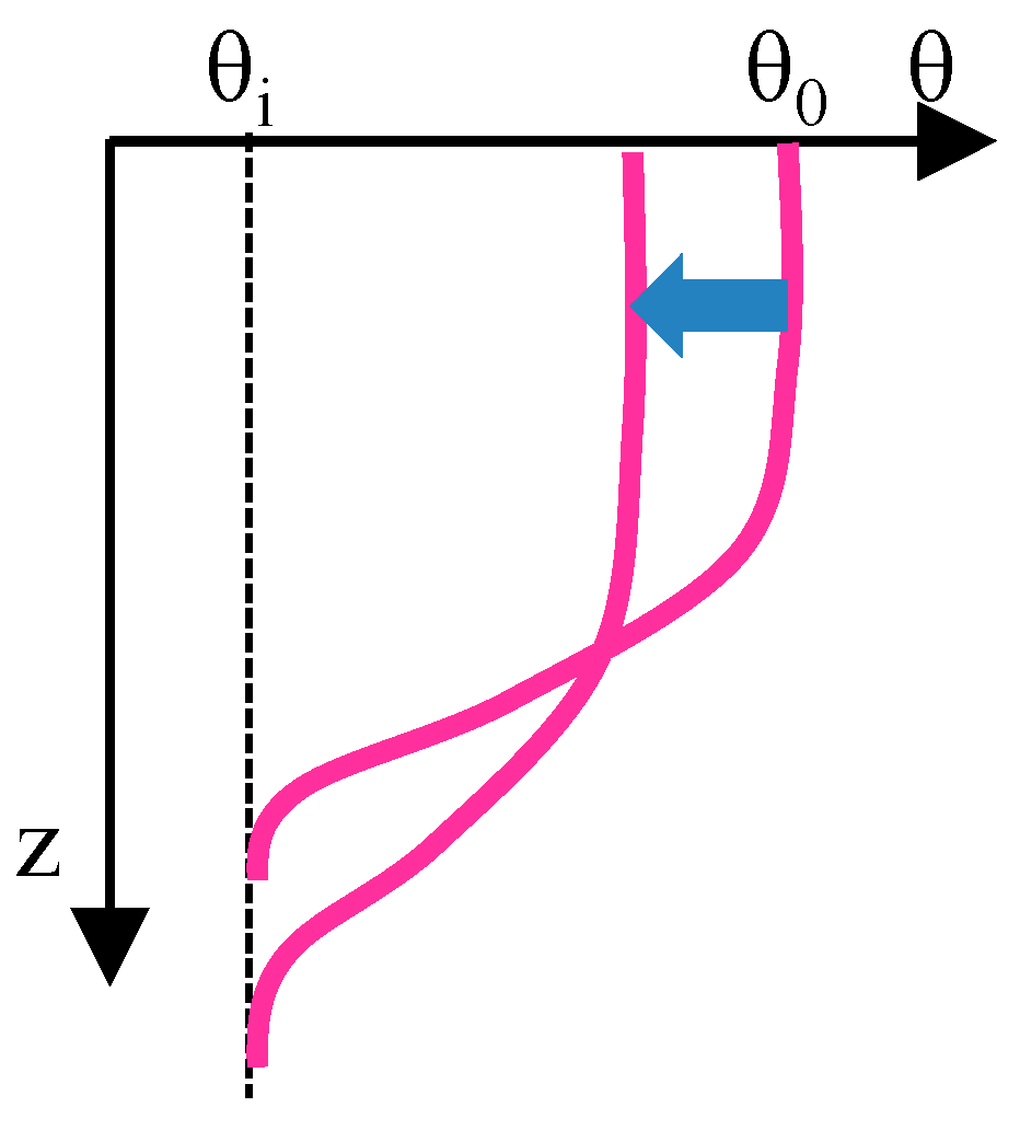
When the hypothesis of uniform initial soil moisture cannot be guaranteed, the models presented in the previous subsections cannot be applied. For complex rainfall patterns involving rainfall hiatus periods or a rainfall rate after time to ponding less than soil infiltration capacity, an approach for the application of the aforementioned classical models was developed [111,112,113] starting from the time compression approximation proposed by Reference [114] for post-hiatus rainfall producing immediate ponding (see also [1]). However, by comparing results with the Richards equation, Reference [22] showed that this approach was not sufficiently accurate because it neglects the soil water redistribution process (Figure 3) which is particularly important when long periods with a light rainfall or a rainfall hiatus occur.
Models combining infiltration and redistribution are therefore the best solution when soils are subjected to complex rainfall patterns, which are prevalent under natural conditions (see also [115,116]). Dagan and Bresler [20] developed an analytical model along this line starting from depth integrated forms of Darcy’s law and the continuity equation and using simplifications in the initial and surface boundary conditions that make easier areal investigations but reduce practical applications at the local scale. In any case, the model is not applicable to local studies with erratic rainfalls producing successive infiltration–redistribution cycles. A more general model was formulated by Reference [26] starting from the same integrated equations, and then combined with a conceptual representation of the wetting soil moisture profile.
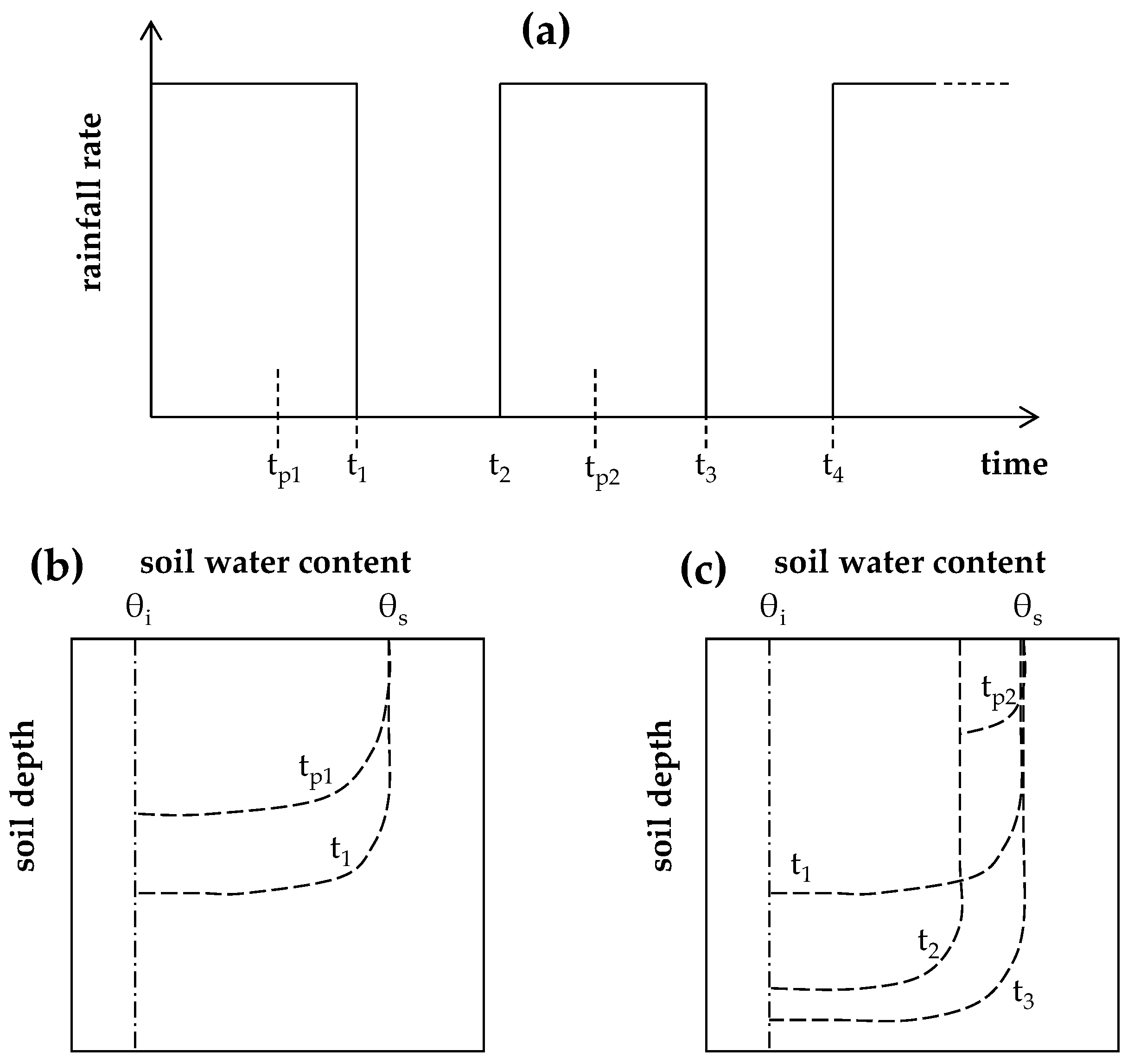
To demonstrate the structure of the model presented in [26], a specific rainfall pattern to describe all the involved components is presented here. The application to erratic rainfall is then a straightforward extension. Let us consider a stepwise rainfall pattern involving successive periods of rainfall with constant r > Ks, separated by periods with r = 0 (see Figure 4). We denote by t1 the duration of the first pulse, t2 and t3, the beginning and end of the second pulse, respectively, and t4 the beginning of the third pulse. The model was derived considering a soil with a constant value of θi and combining the depth-integrated forms of Darcy’s law and the continuity equation. In addition, as the event progresses in time, a dynamic wetting profile, of lowest depth Z and represented by a distorted rectangle through a shape factor β(θ0) ≤ 1, was assumed. The resulting ordinary differential equation is:
where p is a parameter linked with the profile shape of θ and G(θi,θ0) is expressed by Equation (21) modified by the substitution of θs with θ0 and Ks with K0. Equation (23) can be applied for 0 < t < t2, and the profile shape of θ(z) is approximated [23] by:
Functional forms for β and p were obtained by calibration using results provided by the Richards equation applied to a silty loam soil, specifically:
Equation (23) can be solved numerically. For q0 = r, with F′ = (r-Ki)t, it gives θ0(t) until time to ponding, t′p, corresponding to θ0 = θs and dθ0/dt = 0. Then, for t′p < t ≤ t1, with θ0 = θs and dθ0/dt = 0, it provides the infiltration capacity (q0 = fc) and for t1 < t < t2, with q0 = 0, it gives dθ0/dt < 0 thus describing the redistribution process.
The second rainfall pulse leads to a new time to ponding, t″p, but reinfiltration occurs according to two alternative approaches determined by a comparison of r and the downward redistribution rate, DF(t = t2), expressed by:
More specifically, for r ≤ DF, the reinfiltrated water is distributed to the whole dynamic profile and θ0(t) can be still computed by Equation (23), whereas for r > DF, the profile of θ(z, t = t2) is assumed temporarily invariant and starts a superimposed secondary wetting profile which advances alongside the pre-existing profile according to Equation (23) modified by substituting θi with θ0(t2) and F′ with F′2t accumulated for t ≥ t2. If the secondary profile reaches the depth of the first steady one, the compound profile reduces to a single profile and then Equation (23) can be again applied (see Figure 3 for a schematic representation of θ(z,t)). On the other hand, if at t = t3 the secondary profile has not caught up with the first one, redistribution is first applied to the secondary profile and then re-established to the single profile in the successive rainfall hiatus. Finally, in the case at t = t4, the θ(z) profile is still compound and r is larger than DF(t4), and a procedure of consolidation that merges the composite profile is applied early to avoid the formation of a further additional profile.
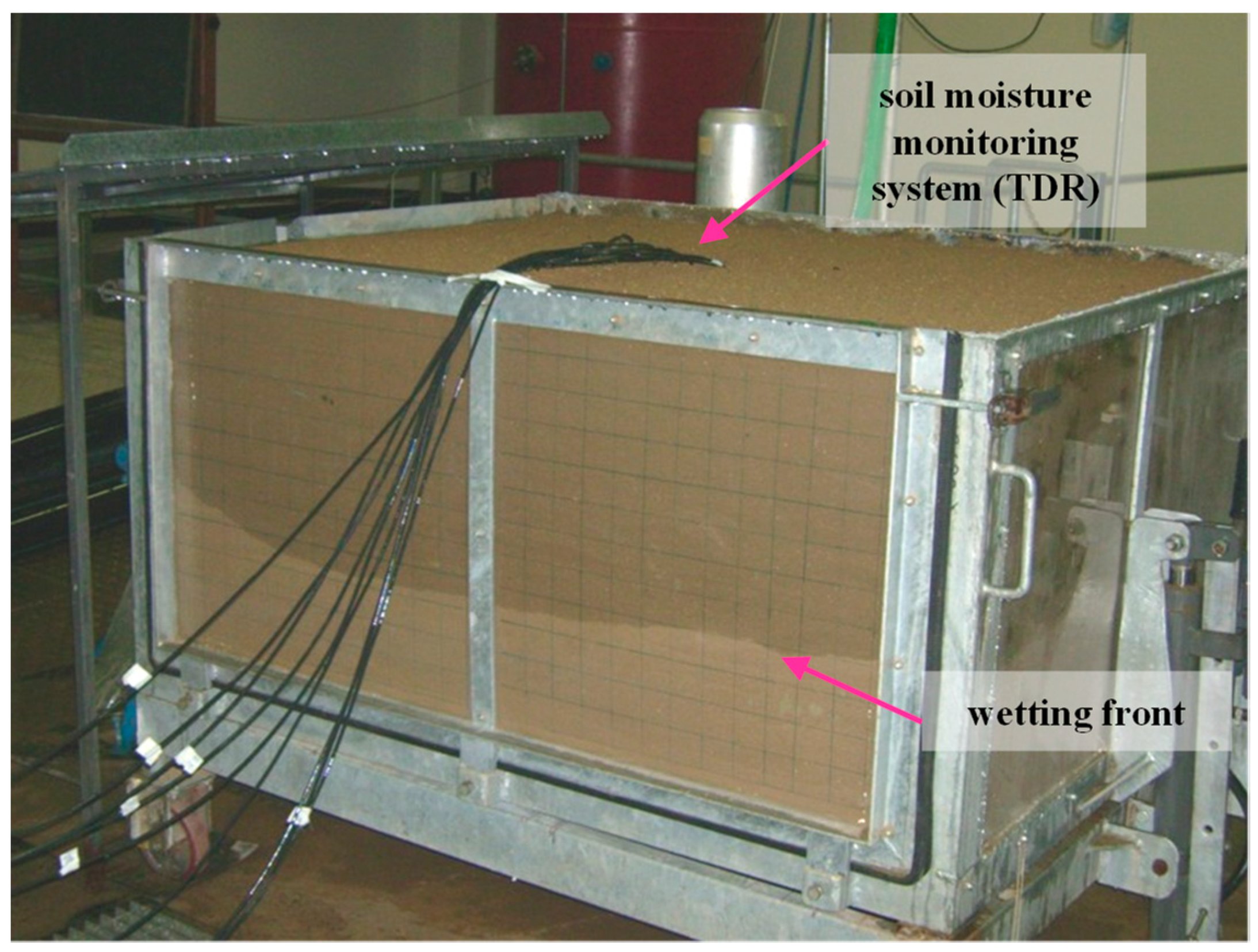
This model incorporates all the components required for application to any natural rainfall pattern. It was calibrated by Reference [26] for a silty loam soil, and then tested using different soils from clay loam to sandy loam soil types. Weighted implicit finite difference solutions of the Richards equation were used as a benchmark. For each soil, the model accuracy was found to be acceptable in terms of both infiltration rate and soil water content, even though better results were obtained for fine-textured soils. In addition, the model was found to simulate fairly well the θ(z,t) profiles observed in laboratory (Figure 5) and field experiments [117,118].
4. Point Infiltration Modeling for Vertically Non-Uniform Soils
A two-layer approximation, with each layer being schematized as homogeneous, is frequently used to set up models of infiltration for natural soils. The process of formation of a sealing layer was accurately examined by References [31,119], and that of disruption was considered by References [120,121,122]. Evidence of the role of crusted soils in semi-arid regions has been recently provided by Reference [123]. Green–Ampt-based models for infiltration into stable crusted soils were proposed by References [33,34,36,39]. An efficient approach that represents transient infiltration into crusted soils was proposed by Reference [40], whereas Reference [41] formulated a model that describes upper-layer dynamics for a ponded upper boundary. On the other hand, vertical profiles with a more permeable upper layer are observed in hydrological practice and can be also used, for example, as a first approximation in the representation of infiltration into homogeneous soils with grassy vegetation [124]. In the latter layering type, the simple model presented by Reference [45] can be usefully applied for infiltration into a saturated soil surface. Under more general conditions, the model by Reference [43] appears to be accurate with modest computational effort.
4.1. Green–Ampt-Based Model for a Layered Soil
A model for infiltration into a two-layered soil with a more permeable upper layer under the condition of continuously saturated soil surface has been formulated by Reference [45]. The classical Green–Ampt equation is applied until the wetting front is in the upper layer, then the following equations are used:
where L2 is the depth of the wetting front below the interface. Equation (27) can be solved at each time for L2 by successive substitutions; L2 is then used in Equations (28) and (29) to determine F and fc, respectively.
4.2. Corradini–Melone–Smith Semi-Analytical/Conceptual Model for a Two-Layered Soil
A semi-analytical/conceptual model applicable to any horizontal two-layered soil where either layer may be more permeable has been formulated by Reference [43]. It relies on the same elements previously used by Reference [26] but adopted here in each layer and integrated at the interface between the two layers by the boundary conditions expressing continuity of flow rate and capillary head (Equations (6a) and (6b)). In addition, at the lower boundary for t > 0, we have ψ2 = ψi. The initial condition is ψ1 = ψ2 = ψi constant at t = 0, and at the interface q(Zc) is approximated through the downward flux in the upper layer as:
where G(ψc,ψ10) is expressed by Equation (21) modified by the substitutions of D(θ)dθ with K(ψ)dψ, θs with ψ10, and θi with ψc. As long as water does not infiltrate in the lower layer, the model presented in [26] is used, then starting from the time tc when the wetting front enters the lower layer, the following system of two ordinary differential equations may be applied:
with and F2 defined as:
and C1(ψ10) = dθ10/dψ10, C1(ψc) = dθ1c/dψ1c. The quantity γ represents a conceptual proportion of the upper layer where θ is increasing due to rainfall and is assumed equal to 0.85 [42], β2 and p2 are determined by Equations (25a–c) but applied using θ20, θ2s, θ2i, and θ2r and substituting r with q(Zc). On the basis of the same stepwise rainfall pattern earlier adopted to explain the model presented in [26], Equations (31) and (32) may be used for tc < t < t2. Then, the two-layer model has to be applied in each layer by analogy with the procedure described for homogeneous soils; in particular, compound and consolidated profiles develop in each layer. In the underlying soil, the generation of additional profiles occurs through q(Zc) in substitution of r. On the basis of the described steps, model application to arbitrary rainfall patterns is straightforward. The solution of the above system, Equations (31) and (32), may be obtained by a library routine for the Runge–Kutta–Verner fifth-order method with a variable time step. Calibration and testing of the model were performed through a comparison with numerical solutions of the Richards equation. Three soils (clay loam, silty loam, and sandy loam) with a variety of thicknesses were combined to realize two-layered soils, where either layer was more permeable, that were selected as test cases. In all instances, the simulations involved the cycle of infiltration–redistribution–reinfiltration. The infiltration rate as well as the water content at the surface and interface were found to be very accurately estimated by the semi-analytical/conceptual model.
5. Areal Infiltration Models over Soil with Variable Hydraulic Properties
At the field scale, considering the significant spatial variability of the main soil hydraulic properties, rainfall infiltration modeling is not analytically tractable, whereas the use of accurate Monte Carlo (M C) simulation techniques imposes an enormous computational burden for routine applications.
In the Introduction section, the evolution of studies for field-scale infiltration models for spatial variability in soil hydraulic properties and rainfall was presented. Models for infiltration at the field scale have been recently developed and represent a useful support for practical hydrological purposes. Two models characterized by significant differences in complexity and application area are presented here.
5.1. Smith and Goodrich Approach
A semi-empirical model to determine the areal-average infiltration rate into areas with random spatial variability of Ks has been proposed by Reference [60]. The authors assumed a lognormal probability density function (PDF) of Ks with a mean value <Ks> and a coefficient of variation CV(Ks), and considered one realization of the random variable. Then, adopting the model presented in [106] (see also [22]) and the Latin Hypercube sampling method, and through a large number of simulations performed for many values of CV(Ks) and rainfall rates, they developed the following effective areal relation for the scaled areal-average infiltration rate, , linked with the corresponding scaled cumulative depth, :
with
where , , and, . The quantity Ke denotes the areal effective value of Ks given by:
where is the PDF of Ks. Finally, Equation (35) may be also applied for r variable with time.
5.2. Govindaraju–Corradini–Morbidelli Semi-Analytical/Conceptual Model
Govindaraju et al. [72] formulated a semi-analytical model to estimate the expected field-scale infiltration rate <In(F)> under the condition of negligible effects of the run-on process. The model incorporates heterogeneity of both Ks and r assumed as random variables with a lognormal and a uniform PDF, respectively. The quantity <In(F)> is estimated through the averaging procedure over the ensemble of two-dimensional realizations of Ks and r. For the sake of simplicity, we first examine the model under a steady-rainfall condition, and then provide the guidelines for applications to a time-varying rainfall rate.
Starting from the extended Green–Ampt model and choosing F as the independent variable, <In(F)> at a given F can be written as:
where fr(r) and are the PDFs of r and Ks, respectively, with Kc which denotes the maximum value of Ks leading to surface saturation in the i-th cell, determined by:
Equation (38) may be expressed as:
with rmin and rmin + R extreme values of the PDF of r and given by:
where Ka and ω stand for the first and the second argument, respectively, of the function. To relate time to F, an implicit relation between the expected value of t, <t>, and F is provided as:
To extend the model by incorporating the run-on effect, an additional empirical term is used in the form presented in [73]:
where tpa is the time to ponding (see Equation (18)) associated with <r> and <Ks>. The parameters a, b, and c are expressed by:
where Equation (44) holds for θi ≪ θs and for θi→θs we have a→0. Furthermore, Equation (46) is undefined for and/or equal to 0. In Equations (43)–(46), length units are in mm and time is expressed in hours.
When the spatial heterogeneity of r can be neglected, with spatially uniform and steady rainfall and negligible run-on, Equations (40) and (42) can be replaced by [61]:
The last formulation was also extended for applications involving r variable in time. The same method can be used to adapt Equations (40) and (42) for unsteady rainfall patterns. Furthermore, the additional empirical term for run-on could be adapted for unsteady rainfalls following the guidelines indicated by Reference [73].
The solution of the model even in the conditions of coupled spatial variability of r and Ks is fairly simple and requires limited computational effort.
The model for coupled heterogeneity of r and Ks (Equations (40), (42), and (43)) was validated by comparison with the results derived starting from MC sampling and using a combination of the extended Green–Ampt formulation at the local scale with the kinematic wave approximation [125] that is required to represent run-on. Through a wide variety of simulations it was shown that: (1) the model produced very accurate estimates of <I> over a clay loam soil and a sandy loam soil; (2) the spatial heterogeneity of both r and Ks can be neglected only when <r> ≫ <K> or for storm durations much greater than tpa; (3) the effects on <I> produced by significant values of CV(Ks) and CV(r) are similar; (4) run-on plays a significant role for moderate storms and high values of CV(Ks) and CV(r); and (5) the model can be simplified using Equations (47) and (48) for CV(r) substantially less than CV(Ks) and steady rainfalls.
6. Conclusions and Open Problems
In spite of the continuous developments in infiltration modeling, challenges regarding infiltration exist for many scales of hydrologic interest. The conflicting results from different studies on the effect of slope on infiltration over homogeneous surfaces show that a solution continues to elude researchers. Careful experimental and theoretical investigations in this regard are needed to fully comprehend this fundamental infiltration behavior over sloping surfaces.
The estimate of infiltration at different spatial scales (i.e., from the local to watershed scales) is a complex problem as further challenges are imposed by the natural spatial variability of soil hydraulic characteristics and that of rainfall. An important issue to be addressed when areal estimates are involved is that concerning the determination of <Ks>, CV(Ks), <r>, and CV(r) together with the corresponding quantities for soil moisture content [126].
The models presented here apply to infiltration into a soil matrix. When macropore flow is significant, the problem becomes much more complicated even though simplified approaches have been proposed. For example, two practical approximations to describe infiltration into soils with macropores rely upon the use of modified values of the saturated hydraulic conductivity of the soil matrix [127] or upon the representation of the two processes of infiltration controlled by the matrix potential and the macropore volume [128]. However, there exist many other models to represent the macropore flow [129], based on the single continuum approach (e.g., [130]), the dual continuum approach, the dual permeability approach (e.g., [131]), and the dual porosity approach (e.g., [132]). Notwithstanding the high number of simplified models, and given the difficulty to investigate the Navier–Stokes equations over finite soil portions, macropore flow still needs a convincing physical theory for the scales of practical interest.
Finally, all these models are formulated for horizontal land surfaces. Extensions of the classical infiltration theory to inclined surfaces were proposed by References [81,87]; however, these theories do not explain the results of laboratory experiments, for example those performed on bare soils in the absence of erosion and a sealing layer [88,92]. The modeling of the slope effects has to be therefore considered as an open problem [97], in particular when surfaces with vegetation are involved [95].
Further challenges exist in our ability to independently measure soil properties at the local scale to identify the true nature of field-scale variability. The use of common measuring instruments for soil hydraulic properties does not yield consistent estimates of variability (e.g., [133]). Both the inter- and intra-instrument errors contribute to a level of uncertainty that has not been understood. Even though measurement techniques are not the topic of this review, measurement errors and uncertainty nevertheless influence modeling efforts that rely on these data. Efforts to appropriately combine disparate measurement results are also needed to realize the full worth of the data that are generated from expensive and time-consuming experimental campaigns.
Field-scale experiments measuring runoff and deep flow are influenced by spatial variability as well, but as yet no theory exists for elucidating the underlying spatial variability from these experiments. Current approaches (e.g., [134]) rely on brute force calibration techniques; however, such methods are often plagued by identifiability and non-uniqueness problems. Moreover, calibration is known to compensate for various model deficiencies, and authors deriving parameter estimates from these approaches must be cognizant of the role played by the underlying model structure. Better conceptual and theoretical underpinnings are needed to move the science of infiltration forward.
Author Contributions
Investigation, Writing—original draft preparation and Writing—review and editing, R.M., C.C., C.S., A.F., J.D., R.S.G.
Funding
This research was partly financed by the Italian Ministry of Education, University and Research (PRIN 2015).
Conflicts of Interest
The authors declare no conflict of interest.
References
- Brutsaert, W. Hydrology—An Introduction; Cambridge University Press: Cambridge, UK, 2005; ISBN 978-0521824798. [Google Scholar]
- Assouline, S. Infiltration into soils: Conceptual approaches and solutions. Water Resour. Res. 2013, 49, 1755–1772. [Google Scholar] [CrossRef] [Green Version]
- Smith, R.E. Infiltration Theory for Hydrologic Applications; Water Resources Monograph; American Geophysical Union: Washington, DC, USA, 2002; Volume 15, ISBN 9780875903194. [Google Scholar]
- Green, W.A.; Ampt, G.A. Studies on soil physics: 1. The flow of air and water through soils. J. Agric. Sci. 1911, 4, 1–24. [Google Scholar] [CrossRef]
- Kostiakov, A.N. On the dynamics of the coefficient of water-percolation in soils and on the necessity for studying it from a dynamic point of view for purposes of amelioration. Trans. Sixth Comm. Int. Soc. Soil Sci. 1932, 1 Pt A, 17–21. [Google Scholar]
- Horton, R.E. An approach toward a physical interpretation of infiltration-capacity. Soil Sci. Soc. Am. J. 1940, 5, 399–417. [Google Scholar] [CrossRef]
- Holtan, H.N. A Concept for Infiltration Estimates in Watershed Engineering; USDA Bulletin: Washington, DC, USA, 1961; pp. 41–51.
- Swartzendruber, D. A quasi solution of Richard equation for downward infiltration of water into soil. Water Resour. Res. 1987, 5, 809–817. [Google Scholar] [CrossRef]
- Philip, J.R. The theory of infiltration: 1. The infiltration equation and its solution. Soil Sci. 1957, 83, 345–357. [Google Scholar] [CrossRef]
- Philip, J.R. The theory of infiltration: 2. The profile at infinity. Soil Sci. 1957, 83, 435–448. [Google Scholar] [CrossRef]
- Philip, J.R. The theory of infiltration: 4. Sorptivity algebraic infiltration equation. Soil Sci. 1957, 84, 257–264. [Google Scholar] [CrossRef]
- Parlange, J.-Y. Theory of water-movement in soils: 2. One-dimensional infiltration. Soil Sci. 1971, 111, 170–174. [Google Scholar] [CrossRef]
- Parlange, J.-Y. Theory of water-movement in soils: 8. One-dimensional infiltration with constant flux at surface. Soil Sci. 1972, 114, 1–4. [Google Scholar] [CrossRef]
- Soil Conservation Service (SCS). National Engineering Handbook; Section 4, Hydrology; USDA: Washington, DC, USA, 1972.
- Brutsaert, W. The concise formulation of diffusive sorption of water in a dry soil. Water Resour. Res. 1976, 12, 1118–1124. [Google Scholar] [CrossRef]
- Brutsaert, W. Vertical infiltration in dry soils. Water Resour. Res. 1977, 13, 363–368. [Google Scholar] [CrossRef]
- Smith, R.E.; Parlange, J.-Y. A parameter-efficient hydrologic infiltration model. Water Resour. Res. 1978, 14, 533–538. [Google Scholar] [CrossRef]
- Broadbridge, P.; White, I. Constant rate rainfall infiltration: A versatile nonlinear model. 1. Analytic solution. Water Resour. Res. 1988, 24, 145–154. [Google Scholar] [CrossRef]
- White, I.; Broadbridge, P. Constant rate rainfall infiltration: A versatile nonlinear model. 2. Application of solutions. Water Resour. Res. 1988, 24, 155–162. [Google Scholar] [CrossRef]
- Dagan, G.; Bresler, E. Unsaturated flow in spatially variable fields. 1. Derivation of models of infiltration and redistribution. Water Resour. Res. 1983, 19, 413–420. [Google Scholar] [CrossRef]
- Haverkamp, R.; Parlange, J.-Y.; Starr, J.L.; Schmitz, G.; Fuentes, C. Infiltration under ponded conditions: 3. A predictive equation based on physical parameters. Soil Sci. 1990, 149, 292–300. [Google Scholar] [CrossRef]
- Smith, R.E.; Corradini, C.; Melone, F. Modeling infiltration for multistorm runoff events. Water Resour. Res. 1993, 29, 133–144. [Google Scholar] [CrossRef]
- Corradini, C.; Melone, F.; Smith, R.E. Modeling infiltration during complex rainfall sequences. Water Resour. Res. 1994, 30, 2777–2784. [Google Scholar] [CrossRef]
- Ross, P.J.; Parlange, J.-Y. Comparing exact and numerical solutions of Richards equation for one-dimensional infiltration and drainage. Soil Sci. 1994, 157, 341–344. [Google Scholar] [CrossRef]
- Barry, D.A.; Parlange, J.-Y.; Haverkamp, R.; Ross, P.J. Infiltration under ponded conditions: 4. An explicit predictive infiltration formula. Soil Sci. 1995, 160, 8–17. [Google Scholar] [CrossRef]
- Corradini, C.; Melone, F.; Smith, R.E. A unified model for infiltration and redistribution during complex rainfall patterns. J. Hydrol. 1997, 192, 104–124. [Google Scholar] [CrossRef]
- Furman, A.; Warrick, A.W.; Zerihun, D.; Sanchez, C.A. Modified Kostiakov infiltration function: Accounting for initial and boundary conditions. J. Irrig. Drain. Eng. 2006, 132, 587–596. [Google Scholar] [CrossRef]
- Wang, K.; Yang, X.; Liu, X.; Liu, C. A simple analytical infiltration model for short-duration rainfall. J. Hydrol. 2017, 555, 141–154. [Google Scholar] [CrossRef]
- Horton, R.E. The role of infiltration in the hydrological cycle. Trans. Am. Geophys. Union 1933, 14, 446–460. [Google Scholar] [CrossRef]
- Horton, R.E. Analysis of runoff plat experiments with varying infiltration capacity. Trans. Am. Geophys. Union 1939, 20, 693–711. [Google Scholar] [CrossRef]
- Mualem, Y.; Assouline, S.; Eltahan, D. Effect of rainfall-induced soil seals on soil water regime: Wetting processes. Water Resour. Res. 1993, 29, 1651–1659. [Google Scholar] [CrossRef]
- Taha, A.; Gresillon, J.M.; Clothier, B.E. Modelling the link between hillslope water movement and stream flow: Application to a small Mediterranean forest watershed. J. Hydrol. 1997, 203, 11–20. [Google Scholar] [CrossRef]
- Hillel, D.; Gardner, W.R. Transient infiltration into crust-topped profile. Soil Sci. 1970, 109, 64–76. [Google Scholar] [CrossRef]
- Ahuja, L.R. Modeling infiltration into surface-sealed soils by the Green-Ampt approach. Soil Sci. Soc. Am. J. 1983, 47, 412–418. [Google Scholar] [CrossRef]
- Beven, K. Infiltration into a class of vertical non-uniform soils. Hydrol. Sci. J. 1984, 29, 425–434. [Google Scholar] [CrossRef]
- Vandervaere, J.-P.; Vauclin, M.; Haverkamp, R.; Peugeot, C.; Thony, J.-L.; Gilfedder, M. Prediction of crust-induced surface runoff with disc infiltrometer data. Soil Sci. 1998, 163, 9–21. [Google Scholar] [CrossRef]
- Selker, J.S.; Duan, J.F.; Parlange, J.-Y. Green and Ampt infiltration into soils of variable pore size with depth. Water Resour. Res. 1999, 35, 1685–1688. [Google Scholar] [CrossRef] [Green Version]
- Chu, X.; Marino, M.A. Determination of ponding condition and infiltration in layered soils under unsteady rainfall. J. Hydrol. 2005, 313, 195–207. [Google Scholar] [CrossRef]
- Moore, I.D. Infiltration equations modified for surface effects. J. Irrig. Drain. Eng. 1981, 107, 71–86. [Google Scholar]
- Smith, R.E. Analysis of infiltration through a two-layer soil profile. Soil Sci. Soc. Am. J. 1990, 54, 1219–1227. [Google Scholar] [CrossRef]
- Philip, J.R. Infiltration into crusted soils. Water Resour. Res. 1998, 34, 1919–1927. [Google Scholar] [CrossRef] [Green Version]
- Smith, R.E.; Corradini, C.; Melone, F. A conceptual model for infiltration and redistribution in crusted soils. Water Resour. Res. 1999, 35, 1385–1393. [Google Scholar] [CrossRef] [Green Version]
- Corradini, C.; Melone, F.; Smith, R.E. Modeling local infiltration for a two layered soil under complex rainfall patterns. J. Hydrol. 2000, 237, 58–73. [Google Scholar] [CrossRef]
- Corradini, C.; Morbidelli, R.; Flammini, A.; Govindaraju, R.S. A parameterized model for local infiltration in two-layered soils with a more permeable upper layer. J. Hydrol. 2011, 396, 221–232. [Google Scholar] [CrossRef]
- Chow, V.T.; Maidment, D.R.; Mays, L.W. Applied Hydrology; McGraw-Hill: New York, NY, USA, 1988; ISBN 978-0071001748. [Google Scholar]
- Nielsen, D.R.; Biggar, J.W.; Erh, K.T. Spatial variability of field measured soil-water properties. Hilgardia 1973, 42, 215–259. [Google Scholar] [CrossRef]
- Warrick, A.W.; Nielsen, D.R. Spatial Variability of Soil Physical Properties in the Field. Applications of Soil Physics; Hillel, D., Ed.; Academic Press: New York, NY, USA, 1980; pp. 319–344. [Google Scholar]
- Peck, A.J. Field variability of soil physical properties. In Advances in Irrigation; Hillel, D., Ed.; Academic: San Diego, CA, USA, 1983; Volume 2, pp. 189–221. ISBN 0-12-024302-4. [Google Scholar]
- Greminger, P.J.; Sud, Y.K.; Nielsen, D.R. Spatial variability of field measured soil-water characteristics. Soil Sci. Soc. Am. J. 1985, 49, 1075–1082. [Google Scholar] [CrossRef]
- Sharma, M.L.; Barron, R.J.W.; Fernie, M.S. Areal distribution of infiltration parameters and some soil physical properties in lateritic catchments. J. Hydrol. 1987, 94, 109–127. [Google Scholar] [CrossRef]
- Loague, K.; Gander, G.A. R-5 revisited, 1. Spatial variability of infiltration on a small rangeland catchment. Water Resour. Res. 1990, 26, 957–971. [Google Scholar] [CrossRef]
- Logsdon, S.D.; Jaynes, D.B. Spatial variability of hydraulic conductivity in a cultivated field at different times. Soil Sci. Soc. Am. J. 1996, 60, 703–709. [Google Scholar] [CrossRef]
- Russo, D.; Bresler, E. Soil hydraulic properties as stochastic processes: 1. Analysis of field spatial variability. Soil Sci. Soc. Am. J. 1981, 45, 682–687. [Google Scholar] [CrossRef]
- Russo, D.; Bresler, E. A univariate versus a multivariate parameter distribution in a stochastic-conceptual analysis of unsaturated flow. Water Resour. Res. 1982, 18, 483–488. [Google Scholar] [CrossRef]
- Sharma, M.L.; Seely, E. Spatial variability and its effect on infiltration. In Proceedings of the Hydrology Water Resources Symposium; Institute of Engineering: Perth, Australia, 1979; pp. 69–73. [Google Scholar]
- Maller, R.A.; Sharma, M.L. An analysis of areal infiltration considering spatial variability. J. Hydrol. 1981, 52, 25–37. [Google Scholar] [CrossRef]
- Saghafian, B.; Julien, P.Y.; Ogden, F.L. Similarity in catchment response: 1. Stationary rainstorms. Water Resour. Res. 1995, 31, 1533–1541. [Google Scholar] [CrossRef]
- Sivapalan, M.; Wood, E.F. Spatial heterogeneity and scale in the infiltration response of catchments. In Scale Problems in Hydrology; Water Science and Technology Library; Gupta, V.K., Rodríguez-Iturbe, I., Wood, E.F., Eds.; D. Reidel Publishing: Dordrecht, Holland, 1986; pp. 81–106. ISBN 978-94-010-8579-3. [Google Scholar]
- McKay, M.D.; Beckman, R.J.; Connover, W.J. A comparison of three methods for selecting values of input variables in the analysis of output from a computer code. Technometrics 1979, 21, 239–245. [Google Scholar] [CrossRef]
- Smith, R.E.; Goodrich, D.C. Model for rainfall excess patterns on randomly heterogeneous area. J. Hydrol. Eng. 2000, 5, 355–362. [Google Scholar] [CrossRef]
- Govindaraju, R.S.; Morbidelli, R.; Corradini, C. Areal infiltration modeling over soils with spatially-correlated hydraulic conductivities. J. Hydrol. Eng. 2001, 6, 150–158. [Google Scholar] [CrossRef]
- Corradini, C.; Govindaraju, R.S.; Morbidelli, R. Simplified modelling of areal average infiltration at the hillslope scale. Hydrol. Proc. 2002, 16, 1757–1770. [Google Scholar] [CrossRef]
- Smith, R.E.; Hebbert, R.H.B. A Monte Carlo analysis of the hydrologic effects of spatial variability of infiltration. Water Resour. Res. 1979, 15, 419–429. [Google Scholar] [CrossRef]
- Woolhiser, D.A.; Smith, R.E.; Giraldez, J.-V. Effects of spatial variability of saturated hydraulic conductivity on Hortonian overland flow. Water Resour. Res. 1996, 32, 671–678. [Google Scholar] [CrossRef]
- Corradini, C.; Morbidelli, R.; Melone, F. On the interaction between infiltration and Hortonian runoff. J. Hydrol. 1998, 204, 52–67. [Google Scholar] [CrossRef]
- Nahar, N.; Govindaraju, R.S.; Corradini, C.; Morbidelli, R. Role of run-on for describing field-scale infiltration and overland flow over spatially variable soils. J. Hydrol. 2004, 286, 36–51. [Google Scholar] [CrossRef]
- Langhans, C.; Govers, G.; Diels, J. Development and parameterization of an infiltration model accounting for water depth and rainfall intensity. Hydrol. Proc. 2013, 27, 3777–3790. [Google Scholar] [CrossRef]
- Goodrich, D.C.; Faurès, J.-M.; Woolhiser, D.A.; Lane, L.J.; Sorooshian, S. Measurement and analysis of small-scale convective storm rainfall variability. J. Hydrol. 1995, 173, 283–308. [Google Scholar] [CrossRef]
- Krajewski, W.F.; Ciach, G.J.; Habib, E. An analysis of small-scale rainfall variability in different climatic regimes. Hydrol. Sci. J. 2003, 48, 151–162. [Google Scholar] [CrossRef] [Green Version]
- Wood, E.F.; Sivapalan, M.; Beven, K. Scale effects in infiltration and runoff production. In Proceedings of the Symposium on Conjunctive Water Use; IAHS: Budapest, Hungary, 1986; ISBN 0-947571-85-X. [Google Scholar]
- Castelli, F. A simplified stochastic model for infiltration into a heterogeneous soil forced by random precipitation. Adv. Water Resour. 1996, 19, 133–144. [Google Scholar] [CrossRef]
- Govindaraju, R.S.; Corradini, C.; Morbidelli, R. A semi-analytical model of expected areal-average infiltration under spatial heterogeneity of rainfall and soil saturated hydraulic conductivity. J. Hydrol. 2006, 316, 184–194. [Google Scholar] [CrossRef]
- Morbidelli, R.; Corradini, C.; Govindaraju, R.S. A field-scale infiltration model accounting for spatial heterogeneity of rainfall and soil saturated hydraulic conductivity. Hydrol. Proc. 2006, 20, 1465–1481. [Google Scholar] [CrossRef]
- Corradini, C.; Flammini, A.; Morbidelli, R.; Govindaraju, R.S. A conceptual model for infiltration in two-layered soils with a more permeable upper layer: From local to field scale. J. Hydrol. 2011, 410, 62–72. [Google Scholar] [CrossRef]
- Govindaraju, R.S.; Corradini, C.; Morbidelli, R. Local and field-scale infiltration into vertically non-uniform soils with spatially-variable surface hydraulic conductivities. Hydrol. Proc. 2012, 26, 3293–3301. [Google Scholar] [CrossRef]
- Beven, K.J. Rainfall-Runoff Modelling; John Wiley & Sons: Hoboken, NJ, USA, 2002; ISBN 978-0-470-71459-1. [Google Scholar]
- Fiori, A.; Romanelli, M.; Cavalli, D.J.; Russo, D. Numerical experiments of streamflow generation in steep catchments. J. Hydrol. 2007, 339, 183–192. [Google Scholar] [CrossRef]
- Nassif, S.H.; Wilson, E.M. The influence of slope and rain intensity on runoff and infiltration. Hydrol. Sci. Bull. 1975, 20, 539–553. [Google Scholar] [CrossRef]
- Sharma, K.; Singh, H.; Pareek, O. Rainwater infiltration into a bar loamy sand. Hydrol. Sci. J. 1983, 28, 417–424. [Google Scholar] [CrossRef]
- Poesen, J. The influence of slope angle on infiltration rate and hortonian overland flow volume. Z. Geomorphol. 1984, 49, 117–131. [Google Scholar]
- Philip, J.R. Hillslope infiltration: Planar slopes. Water Resour. Res. 1991, 27, 109–117. [Google Scholar] [CrossRef]
- Cerdà, A.; García-Fayos, P. The influence of slope angle on sediment, water and seed losses on badland landscapes. Geomorphology 1997, 18, 77–90. [Google Scholar] [CrossRef]
- Fox, D.M.; Bryan, R.B.; Price, A.G. The influence of slope angle on final infiltration rate for interrill conditions. Geoderma 1997, 80, 181–194. [Google Scholar] [CrossRef]
- Chaplot, V.; Le Bissonais, Y. Field measurements of interrill erosion under different slopes and plot sizes. Earth Surf. Process. Landf. 2000, 25, 145–153. [Google Scholar] [CrossRef]
- Janeau, J.L.; Bricquet, J.P.; Planchon, O.; Valentin, C. Soil crusting and infiltration on steep slopes in northern Thailand. Eur. J. Soil Sci. 2003, 54, 543–553. [Google Scholar] [CrossRef]
- Assouline, S.; Ben-Hur, M. Effects of rainfall intensity and slope gradient on the dymanics of interrill erosion during soil surface sealing. Catena 2006, 66, 211–220. [Google Scholar] [CrossRef]
- Chen, L.; Young, M.H. Green-Ampt infiltration model for sloping surfaces. Water Resour. Res. 2006, 42, W07420. [Google Scholar] [CrossRef]
- Essig, E.T.; Corradini, C.; Morbidelli, R.; Govindaraju, R.S. Infiltration and deep flow over sloping surfaces: Comparison of numerical and experimental results. J. Hydrol. 2009, 374, 30–42. [Google Scholar] [CrossRef]
- Ribolzi, O.; Patin, J.; Bresson, L.; Latsachack, K.; Mouche, E.; Sengtaheuanghoung, O.; Silvera, N.; Thiébaux, J.P.; Valentin, C. Impact of slope gradient on soil surface features and infiltration on steep slopes in northern Laos. Geomorphology 2011, 127, 53–63. [Google Scholar] [CrossRef]
- Patin, J.; Mouche, E.; Ribolzi, O.; Chaplot, V.; Sengtaheuanghoung, O.; Latsachak, K.O.; Soulileuth, B.; Valentin, C. Analysis of runoff production at the plot scale during a long-term survey of a small agricultural catchment in Lao PDR. J. Hydrol. 2012, 426–427, 79–92. [Google Scholar] [CrossRef]
- Lv, M.; Hao, Z.; Liu, Z.; Yu, Z. Conditions for lateral downslope unsaturated flow and effects of slope angle on soil moisture movement. J. Hydrol. 2013, 486, 321–333. [Google Scholar] [CrossRef]
- Morbidelli, R.; Saltalippi, C.; Flammini, A.; Cifrodelli, M.; Corradini, C.; Govindaraju, R.S. Infiltration on sloping surfaces: Laboratory experimental evidence and implications for infiltration modelling. J. Hydrol. 2015, 523, 79–85. [Google Scholar] [CrossRef]
- Mu, W.; Yu, F.; Li, C.; Xie, Y.; Tian, J.; Liu, J.; Zhao, N. Effects of rainfall intensity and slope gradient on runoff and soil moisture content on different growing stages of spring maize. Water 2015, 7, 2990–3008. [Google Scholar] [CrossRef]
- Khan, M.N.; Gong, Y.; Hu, T.; Lal, R.; Zheng, J.; Justine, M.F.; Azhar, M.; Che, M.; Zhang, H. Effect of slope, rainfall intensity and mulch on erosion and infiltration under simulated rain on purple soil of south-western Sichuan province, China. Water 2016, 8, 528. [Google Scholar] [CrossRef]
- Morbidelli, R.; Saltalippi, C.; Flammini, A.; Cifrodelli, M.; Picciafuoco, T.; Corradini, C.; Govindaraju, R.S. Laboratory investigation on the role of slope on infiltration over grassy soils. J. Hydrol. 2016, 543, 542–547. [Google Scholar] [CrossRef]
- Wang, J.; Chen, L.; Yu, Z. Modeling rainfall infiltration on hillslopes using flux-concentration relation and time compression approximation. J. Hydrol. 2018, 557, 243–253. [Google Scholar] [CrossRef]
- Morbidelli, R.; Saltalippi, C.; Flammini, A.; Govindaraju, R.S. Role of slope on infiltration: A review. J. Hydrol. 2018, 557, 878–886. [Google Scholar] [CrossRef]
- Gerke, H.H. Preferential flow description for structured soils. J. Plant Nutr. Soil Sci. 2006, 169, 382–400. [Google Scholar] [CrossRef]
- Simunek, J.; Jarvis, N.J.; van Genuchten, M.T.; Gardenas, A. Review and comparison of models describing non-equilibrium and preferential flow and transport in the vadose zone. J. Hydrol. 2003, 272, 14–35. [Google Scholar] [CrossRef]
- Buckingham, E. Studies on the Movement of Soil Moisture; US Department of Agriculture, Bureau of Soils No. 38; USDA: Washington, DC, USA, 1907.
- Brooks, R.H.; Corey, A.T. Hydraulic Properties of Porous Media; Hydrology Paper; Colorado State University: Fort Collins, CO, USA, 1964; Volume 3, p. 27. [Google Scholar]
- Van Genuchten, M.T. A closed-form equation for predicting the hydraulic conductivity of unsaturated soils. Soil Sci. Soc. Am. J. 1980, 44, 892–898. [Google Scholar] [CrossRef]
- Kacimov, A.; Obnosov, Y. Pseudo-hysteretic double-front hiatus-stage soil water parcels supplying a plant-root continuum: The Green-Ampt-Youngs model revisited. Hydrol. Sci. J. 2013, 58, 237–248. [Google Scholar] [CrossRef]
- Mein, R.G.; Larson, C.L. Modeling infiltration during a steady rain. Water Resour. Res. 1973, 9, 384–394. [Google Scholar] [CrossRef]
- Chu, B.T.; Parlange, J.-Y.; Aylor, D.E. Edge effects in linear diffusion. Acta Mech. 1978, 21, 13–27. [Google Scholar] [CrossRef]
- Parlange, J.-Y.; Lisle, I.; Braddock, R.D.; Smith, R.E. The three-parameter infiltration equation. Soil Sci. 1982, 133, 337–341. [Google Scholar] [CrossRef]
- Eagleson, P.S. Dynamic Hydrology; McGraw-Hill: New York, NY, USA, 1970. [Google Scholar]
- Raudkivi, A.J. Hydrology; Pergamon: Oxford, UK, 1979; ISBN 978-0080242613. [Google Scholar]
- Philip, J.R. Theory of infiltration. In Advances in Hydroscience; Chow, W.T., Ed.; Academic Press: New York, NY, USA, 1969; Volume 5, pp. 215–296. [Google Scholar]
- Youngs, E.G. An infiltration method measuring the hydraulic conductivity of unsaturated porous materials. Soil Sci. 1964, 97, 307–311. [Google Scholar] [CrossRef]
- Mls, J. Effective rainfall estimation. J. Hydrol. 1980, 45, 305–311. [Google Scholar] [CrossRef]
- Péschke, G.; Kutilek, M. Infiltration model in simulated hydrographs. J. Hydrol. 1982, 56, 369–379. [Google Scholar] [CrossRef]
- Verma, S.C. Modified Horton’s infiltration equation. J. Hydrol. 1982, 58, 383–388. [Google Scholar] [CrossRef]
- Reeves, M.; Miller, E.E. Estimating infiltration for erratic rainfall. Water Resour. Res. 1975, 11, 102–110. [Google Scholar] [CrossRef]
- Basha, H.A. Infiltration models for semi-infinite soil profiles. Water Resour. Res. 2011, 47, W08516. [Google Scholar] [CrossRef]
- Basha, H.A. Infiltration models for soil profiles bounded by a water table. Water Resour. Res. 2011, 47, W10527. [Google Scholar] [CrossRef]
- Melone, F.; Corradini, C.; Morbidelli, R.; Saltalippi, C. Laboratory experimental check of a conceptual model for infiltration under complex rainfall patterns. Hydrol. Proc. 2006, 20, 439–452. [Google Scholar] [CrossRef]
- Melone, F.; Corradini, C.; Morbidelli, R.; Saltalippi, C.; Flammini, A. Comparison of theoretical and experimental soil moisture profiles under complex rainfall patterns. J. Hydrol. Eng. 2008, 13, 1170–1176. [Google Scholar] [CrossRef]
- Mualem, Y.; Assouline, S. Modeling soil seal as a nonuniform layer. Water Resour. Res. 1989, 25, 2101–2108. [Google Scholar] [CrossRef]
- Bullock, M.S.; Temper, W.D.; Nelson, S.D. Soil cohesion as affected by freezing, water content, time and tillage. Soil Sci. Soc. Am. J. 1988, 52, 770–776. [Google Scholar] [CrossRef]
- Emmerich, W.E. Season and erosion pavement influence on saturated soil hydraulic conductivity. Soil Sci. 2003, 168, 637–645. [Google Scholar] [CrossRef]
- Morbidelli, R.; Corradini, C.; Saltalippi, C.; Flammini, A.; Rossi, E. Infiltration-soil moisture redistribution under natural conditions: Experimental evidence as a guideline for realizing simulation models. Hydrol. Earth Syst. Sci. 2011, 15, 2937–2945. [Google Scholar] [CrossRef]
- Chen, L.; Sela, S.; Svoray, T.; Assouline, S. The role of soil-surface sealing, microtopography, and vegetation patches in rainfall-runoff processes in semiarid areas. Water Resour. Res. 2013, 49, 5585–5599. [Google Scholar] [CrossRef] [Green Version]
- Morbidelli, R.; Saltalippi, C.; Flammini, A.; Rossi, E.; Corradini, C. Soil water content vertical profiles under natural conditions: Matching of experiments and simulations by a conceptual model. Hydrol. Proc. 2014, 28, 4732–4742. [Google Scholar] [CrossRef]
- Singh, V.P. Kinematic Wave Modeling in Water Resources: Surface Water Hydrology; John Wiley & Sons: New York, NY, USA, 1996; ISBN 0-471-10945-2. [Google Scholar]
- Morbidelli, R.; Corradini, C.; Saltalippi, C.; Brocca, L. Initial soil water content as input to field-scale infiltration and surface runoff models. Water Resour. Manag. 2012, 26, 1793–1807. [Google Scholar] [CrossRef]
- Maidment, D.R. Handbook of Hydrology; McGraw-Hill: New York, NY, USA, 1993; ISBN 9780070397323. [Google Scholar]
- Bronstert, A.; Bardossy, A. The role of spatial variability of soil moisture for modelling surface runoff generation at the small catchment scale. Hydrol. Earth Syst. Sci. 1999, 3, 505–516. [Google Scholar] [CrossRef]
- Beven, K.; Germann, P. Macropores and water flow in soils revisited. Water Resour. Res. 2013, 49, 3071–3092. [Google Scholar] [CrossRef] [Green Version]
- Simunek, J.; van Genuchten, M.T. Modeling nonequilibrium flow and transport processes using HYDRUS. Vadose Zone J. 2008, 7, 782–797. [Google Scholar] [CrossRef]
- Ireson, A.M.; Butler, A.P. Controls on preferential recharge to Chalk aquifers. J. Hydrol. 2011, 398, 109–123. [Google Scholar] [CrossRef] [Green Version]
- Van Dam, J.C.; Groenendijk, P.; Hendriks, R.F.A.; Kroes, J.G. Advances of modeling water flow in variability saturated soils with SWAP. Vadose Zone J. 2008, 7, 640–653. [Google Scholar] [CrossRef]
- Morbidelli, R.; Saltalippi, C.; Flammini, A.; Cifrodelli, M.; Picciafuoco, T.; Corradini, C.; Govindaraju, R.S. In-situ measurements of soil saturated hydraulic conductivity: Assessment of reliability through rainfall-runoff experiments. Hydrol. Proc. 2017, 31, 3084–3094. [Google Scholar] [CrossRef]
- Flammini, A.; Morbidelli, R.; Saltalippi, C.M.; Picciafuoco, T.; Corradini, C.; Govindaraju, R.S. Reassessment of a semi-analytical field-scale infiltration model through experiments under natural rainfall events. J. Hydrol. 2018, 565, 835–845. [Google Scholar] [CrossRef]
Figure 1.
Infiltration capacity, IC(t), and infiltration rate, f(t), of a silty loam soil under a natural rainfall event (observed in Central Italy) characterized by a variable intensity, r(t).
Figure 1.
Infiltration capacity, IC(t), and infiltration rate, f(t), of a silty loam soil under a natural rainfall event (observed in Central Italy) characterized by a variable intensity, r(t).

Figure 2.
Graphical representation of the Horton empirical equation.

Figure 3.
Graphical representation of the soil water redistribution process.

Figure 4.
(a) Rainfall pattern selected to describe the Corradini–Melone–Smith semi-analytical model for point infiltration. (b,c) Profiles of soil water content at various times indicated in (a) and associated with different infiltration-redistribution stages. For symbols, see the text.
Figure 4.
(a) Rainfall pattern selected to describe the Corradini–Melone–Smith semi-analytical model for point infiltration. (b,c) Profiles of soil water content at various times indicated in (a) and associated with different infiltration-redistribution stages. For symbols, see the text.


© 2018 by the authors. Licensee MDPI, Basel, Switzerland. This article is an open access article distributed under the terms and conditions of the Creative Commons Attribution (CC BY) license (http://creativecommons.org/licenses/by/4.0/).
Share and Cite
MDPI and ACS Style
Morbidelli, R.; Corradini, C.; Saltalippi, C.; Flammini, A.; Dari, J.; Govindaraju, R.S. Rainfall Infiltration Modeling: A Review. Water 2018, 10, 1873. https://doi.org/10.3390/w10121873
AMA Style
Morbidelli R, Corradini C, Saltalippi C, Flammini A, Dari J, Govindaraju RS. Rainfall Infiltration Modeling: A Review. Water. 2018; 10(12):1873. https://doi.org/10.3390/w10121873
Chicago/Turabian StyleMorbidelli, Renato, Corrado Corradini, Carla Saltalippi, Alessia Flammini, Jacopo Dari, and Rao S. Govindaraju. 2018. "Rainfall Infiltration Modeling: A Review" Water 10, no. 12: 1873. https://doi.org/10.3390/w10121873
Note that from the first issue of 2016, this journal uses article numbers instead of page numbers. See further details here.