Ranking of CMIP5 GCM Skills in Simulating Observed Precipitation over the Lower Mekong Basin, Using an Improved Score-Based Method

Abstract

This study assessed the performances of 34 Coupled Model Intercomparison Project Phase 5 (CMIP5) general circulation models (GCMs) in reproducing observed precipitation over the Lower Mekong Basin (LMB). Observations from gauge-based data of the Asian Precipitation-Highly Resolved Observational Data Integration Towards Evaluation of Water Resources (APHRODITE) precipitation data were obtained from 1975 to 2004. An improved score-based method was used to rank the performance of the GCMs in reproducing the observed precipitation over the LMB. The results revealed that most GCMs effectively reproduced precipitation patterns for the mean annual cycle, but they generally overestimated the observed precipitation. The GCMs showed good ability in reproducing the time series characteristics of precipitation for the annual period compared to those for the wet and dry seasons. Meanwhile, the GCMs obviously reproduced the spatial characteristics of precipitation for the dry season better than those for annual time and the wet season. More than 50% of the GCMs failed to reproduce the positive trend of the observed precipitation for the wet season and the dry season (approximately 52.9% and 64.7%, respectively), and approximately 44.1% of the GCMs failed to reproduce positive trend for annual time over the LMB. Furthermore, it was also revealed that there existed different robust criteria for assessing the GCMs’ performances at a seasonal scale, and using multiple criteria was superior to a single criterion in assessing the GCMs’ performances. Overall, the better-performed GCMs were obtained, which can provide useful information for future precipitation projection and policy-making over the LMB.

1. Introduction

Precipitation is a key climate variable in studying the effects of climate change [1]. Changes in precipitation patterns induced by climate change directly or indirectly cause variations in the hydrological cycle and ecological system, as well as in socioeconomic development and human health [2,3,4,5]. Under the business-as-usual (BAU) scenario, the world will face a 40% water deficit by 2030 [6]. Therefore, climate change poses severe challenges for humans in facing their existence and development. Thus, climate change assessments have been conducted through precipitation simulations, and the response measures to climate change effects have appeared to be particularly significant.

General circulation models (GCMs) are valuable tools for studying past, present, and future climate trends and variability [7,8]. The fifth phase of the Coupled Model Intercomparison Project 5 (CMIP5) of the World Climate Research Programme (WCRP) provided numerical numbers of GCMs compared to CMIP3 GCMs to enhance the understanding of the mechanisms of climate system change and to improve the capability to simulate climate change [9,10,11,12]. For example, Sperber et al. 2013 [9] showed that the CMIP5 multimodel mean (MMM) had better skills in simulating pattern correlations with respect to observations than the CMIP3 MMM did. Sillmann et al. 2013 [10] found that there existed some improvements of the CMIP5 ensemble in the representation of the magnitude of precipitation indices compared to the CMIP3. Meher et al. 2017 [12] showed that CMIP5 GCMs were more skillful in simulating the annual cycle of interannual variability of precipitation compared to CMIP3 GCMs over the Western Himalayan Region. Additionally, a study by Hasson et al. 2016 [13] showed that CMIP5 GCMs had improved skills in describing the seasonality of precipitation regimes compared to their predecessors over the Asian monsoon region, which includes the Mekong River Basin, but the performance of the GCMs varied for different river basins. Because of the existence of uncertainty in precipitation simulations, it is necessary to know how well GCMs can effectively simulate precipitation on a regional scale such as the river basin before projecting future climate change.

Numerous scholars have assessed the performance of the CMIP5 GCMs in simulating precipitation at the global scale [14,15,16,17,18], regional scale [11,19,20,21], and subregional scale [12,22,23,24]. Thus far, the multimodel ensembles of CMIP5 for projection of climate variables have been effectively used [20], and some authors consider these ensembles to be better than individual GCM [25]. However, some studies have suggested that multimodel ensembles are deficient in their projection [14,26], and thus it may be essential to consider acceptable GCMs for specific assessments rather than simple multimodel ensembles [8]. Moreover, ensemble methods could be applied on the best-performing GCMs [21]. Thus, assessing the performance of GCMs also provided useful information for future climate change studies with respect to the application of multimodel ensembles.

Climate change may increase the frequency and intensity of extreme hydrological events, as well as the frequency of years with above-normal monsoons or extremely low precipitation [27]. In the past few decades, the demand for water resources has increased with population growth and economic development [28]. Moreover, further increases in population and accelerated urbanization have exacerbated the demand for water resources [29]. Additionally, changes in precipitation are likely to have great impacts on the water cycle system, water resources, and agricultural production of the Lower Mekong Basin (LMB) [5,30,31]. Therefore, assessing GCM performances in simulating precipitation is essential for future precipitation change and policy-making over the LMB. In previous studies, assessing GCM performance has been mainly based on satellite data rather than gauge-based data [17,24,32,33], and the same for the LMB [13]. However, satellite data likely underestimated observed precipitation over the Mekong River Basin [34]. Thus, we used gauge-based data of the Asian Precipitation-Highly Resolved Observational Data Integration Towards Evaluation of Water Resources (APHRODITE) [35] as the observational data for assessing GCM performance over the LMB.

In addition, few studies have focused on the CMIP5 GCM assessments at a river basin of the Asian monsoon regions such as the LMB, as well as dividing the time scales into the wet season, dry season, and annual time to make comprehensive assessments. Therefore, this study assessed the performance of CMIP5 GCMs in simulating observed precipitation over the LMB to provide useful guidance for the assessment of climate change effects.

2. Materials and Methods

2.1. Study Area

The Lower Mekong Basin (Figure 1) is located in Southeast Asia within the countries of Laos, Thailand, Cambodia, and Vietnam [36]. It has a catchment area of about 630,000 km², with a total length of about 2668 km. The climate of this area belongs to the tropical monsoon climate, with the wet season from May to October, and the dry season from November to the following April. Mean annual precipitation ranges from less than 1000 mm in northeast Thailand to more than 3500 mm in north-central Laos [37]. High terrain is predominant in the Laos, whereas flat terrain is predominant in northeast Thailand, Cambodia, and the delta in Vietnam (Figure 1).

2.2. GCM Data

Thirty-four GCMs from CMIP5 were used in this study [38], including precipitation outputs, specific humidity, and wind (eastward wind and northward wind) data from 1975 to 2004.

Table 1. Basic information of the Coupled Model Intercomparison Project 5 (CMIP5) models used in this study.

Model Name	ID	Institution	Resolution (Lon × Lat)	Time Range
ACCESS1.0	1	Commonwealth Scientific and Industrial Research Organization/Bureau of Meteorology, Australia	1.88° × 1.25°	1850–2005
ACCESS1.3	2		1.88° × 1.25°	1850–2005
BCC-CSM1.1	3	Beijing Climate Center, China Meteorological Administration, China	2.81° × 2.79°	1850–2012
BNU-ESM	4	College of Global Change and Earth System Science, Beijing Normal University, China	2.81° × 2.79°	1850–2005
CanESM2	5	Canadian Centre for Climate Modelling and Analysis, Canada	2.81° × 2.79°	1850–2005
CCSM4	6	National Center for Atmospheric Research, USA	1.25° × 0.94°	1850–2005
CESM1(CAM5)	7		1.25° × 0.94°	1850–2005
CESM1(WACCM)	8		2.50° × 1.88°	1850–2005
CMCC-CMS	9	Centro Euro-Mediterraneo sui Cambiamenti Climatici, Italy	1.88° × 1.88°	1850–2005
CNRM-CM5	10	Centre National de Recherches Météorologiques Centre Européen de Recherche et Formation Avancée en Calcul Scientifique, France	1.41° × 1.40°	1850–2005
CSIRO-Mk3.6.0	11	Commonwealth Scientific and Industrial Research Organization/Queensland Climate Change Centre of Excellence, Australia	1.88° × 1.88°	1850–2005
EC-EARTH	12	EC-EARTH consortium published at the Irish Centre for High-End Computing, Netherlands/Ireland	1.13° × 1.13°	1850–2009
FGOALS-g2	13	Institute of Atmospheric Physics, Chinese Academy of Sciences, China	2.81° × 2.81°	1850–2005
FIO-ESM	14	The First Institute of Oceanography, SOA, China	2.80° × 2.80°	1850–2005
GFDL-CM3	15	NOAA Geophysical Fluid Dynamics Laboratory, USA	2.50° × 2.00°	1860–2005
GFDL-ESM2G	16		2.00° × 2.02°	1861–2005
GFDL-ESM2M	17		2.50° × 2.02°	1861–2005
GISS-E2-H	18	NASA/GISS Goddard Institute for Space Studies, USA	2.50° × 2.00°	1850–2005
GISS-E2-R	19		2.50° × 2.00°	1850–2005
HadGEM2-AO	20	National Institute of Meteorological Research, Korea Meteorological Administration, Korea	1.88° × 1.25°	1860–2005
HadGEM2-CC	21	Met Office Hadley Center, UK	1.88° × 1.25°	1859–2005
HadGEM2-ES	22		1.88° × 1.25°	1859–2005
INMCM4.0	23	Russian Academy of Sciences, Institute for Numerical Mathematics, Russia	2.00° × 1.50°	1850–2005
IPSL-CM5A-LR	24	Institute Pierre-Simon Laplace, France	3.75° × 1.89°	1850–2005
IPSL-CM5A-MR	25		2.50° × 1.27°	1850–2005
IPSL-CM5B-LR	26		3.75° × 1.89°	1850–2005
MIROC4h	27	Atmosphere and Ocean Research Institute (the University of Tokyo), National Institute for Environmental Studies, and Japan Agency for Marine-Earth Science and Technology, Japan	0.56° × 0.56°	1950–2005
MIROC5	28		1.41° × 1.40°	1850–2012
MIROC-ESM	29		2.81° × 2.79°	1850–2005
MIROC-ESM-CHEM	30		2.81° × 2.79°	1850–2005
MPI-ESM-LR	31	Max Planck Institute for Meteorology, Germany	1.88° × 1.87°	1850–2005
MPI-ESM-MR	32		1.88° × 1.87°	1850–2005
MRI-CGCM3	33	Meteorological Research Institute, Japan	1.13° × 1.12°	1850–2005
NorESM1-M	34	Bjerknes Centre for Climate Research, Norwegian Climate Center, Norway	2.50° × 1.89°	1850–2005

gives an overview of the home institution of the models and their resolution. Further details can be found at the CMIP5 website (http://cmip-pcmdi.llnl.gov/cmip5/index.html).

2.3. Precipitation Data

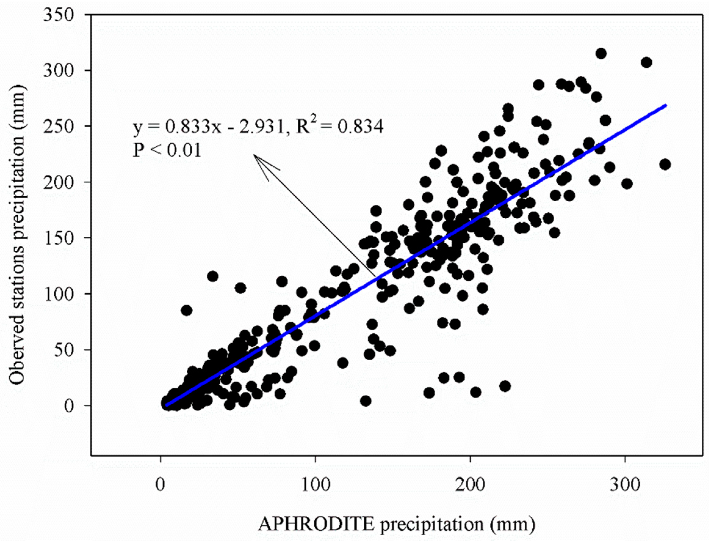
This study used gauge-based data of the APHRODITE precipitation data as the observational data. APHRODITE precipitation data are gauge-based daily data, with a high horizontal resolution of 0.25° × 0.25° [35]. APHRODITE has been proven to be a better-gridded precipitation product for the Mekong River Basin, contributing to studies such as climate change, Asian water resources, statistical downscaling, forecast improvements, verification of numerical model simulation, and satellite precipitation estimates [34]. Daily precipitation data of the observed stations from the Global Surface Summary of the Day (GSOD) and the Global Historical Climatology Network (GHCN) were obtained from the National Climatic Data Center (https://gis.ncdc.noaa.gov). Precipitation of the APHRODITE, GSOD, and GHCN were calculated for monthly data. As shown in Figure 2, monthly precipitation of GSOD and GHCN showed significant correlation with APHRODITE precipitation at a significance of 0.01, with an R-squared (R²) of 0.834, indicating that APHRODITE precipitation was suitable for assessing the GCMs’ performances over the LMB.

Due to the various resolutions of the GCMs and the observations, monthly precipitation outputs for all of the GCMs and APHRODITE precipitation data were converted to 2.5 × 2.5 grid using bilinear interpolation, and 21 grids were selected for comparison (Figure 1). In this study, we considered 1975–2004 as the reference period, including the periods of annual time, January to December; the wet season, May to October; and the dry season, November to the following April. As for the APHRODITE precipitation, precipitation of the mean wet season and dry season was 1213.8 mm and 216.9 mm, which accounted for approximately 86.1% and 13.9% the annual precipitation over the LMB. The sample size for the annual time, the wet season, and the dry season were 360, 180, and 180, respectively. The LMB precipitation data were calculated by taking the arithmetic mean of the 21 grids.

2.4. National Centers for Environmental Prediction (NCEP) Reanalysis Data

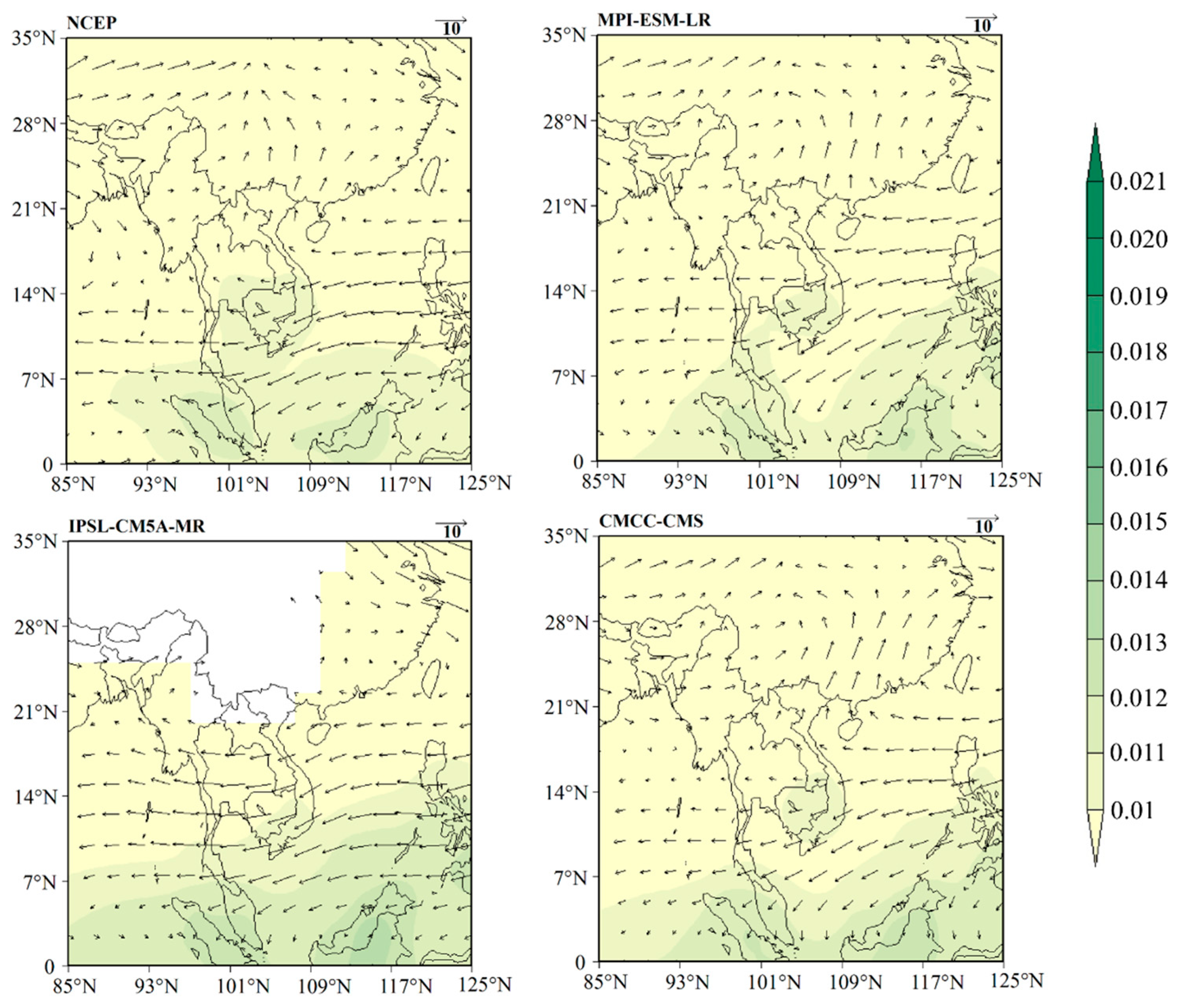
Monthly specific humidity and wind data were used from NCEP reanalysis data (https://www.esrl.noaa.gov/psd/) from 1975 to 2004. In order to explain the differences of precipitation simulation over the LMB, we explored the three best-ranked GCMs (overall results) in reproducing the main features of atmospheric circulation over the LMB. Spatial distributions of mean monthly specific humidity and wind at the 850 hPa level for the wet season and the dry season of the period 1975–2004 over the LMB were calculated to make comparisons with the corresponding results from the NCEP reanalysis data.

2.5. Methods

Multiple criteria were used for the assessment, including root mean square error (RMSE), percentage bias (PBIAS), linear correlation coefficient (r) for monthly series and for spatial distribution, the Mann–Kendall test statistic (Z), Sen’s slope, the Brier score (BS), and the significance score (S_score). The main assessment steps were as follows:

First, we calculated the statistics of the eight criteria. Then, based on the statistics of the criteria, we used an improved rank score (RS) method [39] to calculate the ranking scores of the GCMs’ performances by a single criterion. Finally, the overall ranking scores of the GCMs’ performances were calculated using ranking scores of the GCMs’ performances by multiple criteria. The specific calculation methods were as follows:

RMSE, a common way for representing the difference between the GCM and the observed values, was defined as follows:

$$\mathrm{RMSE}=\sqrt{\frac{{\sum }_{\mathrm{i}=1}^{\mathrm{n}}{\left(\mathrm{pmi}-\mathrm{poi}\right)}^2}{\mathrm{n}}}$$

(1)

where pmi and poi represent the monthly precipitation for the GCM and the observed value of the LMB at i time step, respectively, and n represents the total number of the time steps. A smaller RMSE value indicated a relatively better performance of a GCM.

The PBIAS was used to represent the tendency of the difference between the GCM and the observed values, and was defined as follows:

$$\mathrm{PBIAS}(\%)=\frac{{\sum }_{\mathrm{i}=1}^{\mathrm{n}}\left(\mathrm{pmi}-\mathrm{poi}\right)}{{\sum }_{\mathrm{i}=1}^{\mathrm{n}}\mathrm{poi}}\times 100$$

(2)

The variables in the formula are the same as those described in Equation (1). A PBIAS value closer to zero indicated a relatively better performance of a GCM.

The linear correlation coefficient (r) was used to assess both the monthly series and spatial distribution of precipitation between the observation and GCMs. For the monthly series correlation coefficient (r), the correlation coefficient was calculated between observed and modeled long-term monthly mean values, and the sample sizes were 6, 6, and 12 for the wet season, dry season, and annual time, respectively. For the spatial distribution correlation coefficient (r), the sample sizes were 21 for all the three time periods, and r was calculated according to the 21 grids based on the observation and GCMs, including the mean annual values, mean values for the annual wet season, and mean values for the annual dry season. The formula was defined as follows:

$$\mathrm{r}=\frac{{\sum }_{\mathrm{i}=1}^{\mathrm{n}}\left(\mathrm{pmi}-\mathrm{p}\overline{\mathrm{m}}\right)\left(\mathrm{poi}-\mathrm{p}\overline{\mathrm{o}}\right)}{\sqrt{{\sum }_{\mathrm{i}=1}^{\mathrm{n}}{\left(\mathrm{pmi}-\mathrm{p}\overline{\mathrm{m}}\right)}^2\times {\sum }_{\mathrm{i}=1}^{\mathrm{n}}{\left(\mathrm{poi}-\mathrm{p}\overline{\mathrm{o}}\right)}^2}}$$

(3)

Here, for the monthly series correlation coefficient (r), pmi and poi represent the monthly precipitation for the GCM and the observation of the LMB at i month, respectively, and the $\mathrm{p}\overline{\mathrm{m}}$ and $\mathrm{p}\overline{\mathrm{o}}$ represent the mean values for precipitation of the GCM and the observation, respectively. For the spatial distribution correlation coefficient (r), pmi and poi represent precipitation for the GCM and the observation of the mean annual values, mean values for the annual wet season, or mean values for the annual dry season at i grid, respectively, and $\mathrm{p}\overline{\mathrm{m}}$ and $\mathrm{p}\overline{\mathrm{o}}$ represent the corresponding mean values for precipitation of the GCM and the observation of all grids, respectively. A larger value of r indicated a relatively better performance of a GCM.

The Mann–Kendall test statistic (Z) and Sen’s slope were used to obtain the trends and their magnitudes for GCMs and observation. Thus, the effectiveness of the GCMs in representing the observed trends could be determined. We used the annual time series for the analysis, which included the annual wet season values, annual dry season values, and annual values, which we attributed to the wet season, dry season, and annual time for this analysis, respectively.

The Mann–Kendall test statistic (Z) is defined as follows [40]:

$$\mathrm{Z}=\{\begin{array}{c}\frac{\mathrm{S}-1}{\sqrt{\mathrm{v}\mathrm{a}\mathrm{r}\left(\mathrm{S}\right)}},\mathrm{S}>0\\ 0,\mathrm{S}=0\\ \frac{\mathrm{S}+1}{\sqrt{\mathrm{v}\mathrm{a}\mathrm{r}\left(\mathrm{S}\right)}},\mathrm{S}<0\end{array}$$

(4)

$$\mathrm{S}={\sum }_{\mathrm{i}=1}^{\mathrm{n}-1}{\sum }_{\mathrm{k}=\mathrm{i}+1}^{\mathrm{n}}\mathrm{sgn}({\mathrm{x}}_{\mathrm{k}}-{\mathrm{x}}_{\mathrm{i}})$$

(5)

Here x_k and x_i are the sequential precipitation values, n is the length (29) of the dataset,

$$\mathrm{sgn}\left(\mathsf{\theta }\right)=\{\begin{array}{c}1, \mathsf{\theta }>0\\ 0, \mathsf{\theta }=0\\ -1, \mathsf{\theta }<0\end{array}$$

(6)

and

$$\mathrm{var}\left[\mathrm{S}\right]=\left[\mathrm{n}\left(\mathrm{n}-1\right)\left(2\mathrm{n}+5\right)-\sum _{\mathrm{t}}\mathrm{t}(\mathrm{t}-1)(2\mathrm{t}+5)\right]/18$$

(7)

where t is the extent of any given tie, and ∑ denotes the summation over all ties.

Sen’s slope was defined as follows [41,42]:

$$\mathsf{\beta }=\mathrm{Median}\left(\frac{{\mathrm{x}}_{\mathrm{i}}-{\mathrm{x}}_{\mathrm{j}}}{\mathrm{i}-\mathrm{j}}\right),{\forall }_{\mathrm{j}}<\mathrm{i}$$

(8)

where 1 < j < i < n, and the slope estimator β represents the median of the entire data set.

The BS and S_score were used to assess the GCM probability density functions (PDFs) of monthly precipitation. The formulas were defined as follows:

$$\mathrm{BS}=\frac{{\sum }_{\mathrm{i}=1}^{\mathrm{n}}{\left(\mathrm{B}\mathrm{m}\mathrm{i}-\mathrm{B}\mathrm{o}\mathrm{i}\right)}^2}{\mathrm{n}}$$

(9)

$${\mathrm{S}}_{\mathrm{score}}={\sum }_{\mathrm{i}=1}^{\mathrm{n}}\mathrm{M}\mathrm{i}\mathrm{n}\mathrm{i}\mathrm{m}\mathrm{u}\mathrm{m}\left(\mathrm{B}\mathrm{m}\mathrm{i},\mathrm{B}\mathrm{o}\mathrm{i}\right)$$

(10)

Here, Bmi and Boi represent the probability of the GCM and observed values at the ith of each bin, respectively, and n is the number of bins, which was set as 30 according to the data range. BS is a measurement of mean squared error for probability prediction [43], and S_score is a measurement of the degree of overlap between the simulated probability distribution and the observed value [44]. Thus, a smaller BS value and a larger S_score value indicated relatively better performance of a GCM [45].

As for the RS method, a smaller RMSE value for the relative error indicates better performance of a GCM, as does a larger r value of the non-error index for the correlation coefficient (r), which can easily lead to inconsistent assessment results [39,45]. The improved RS distinguished the inconsistency between the relative error index and the nonrelative error index, which could be used for the assessment of multiple criteria and climatic variables to synthetically assess the performance of GCMs in applicable regions [39]. The improved RS of each assessment criterion could be calculated according to its statistic as follows [39]:

$$\mathrm{R}{\mathrm{S}}_{\mathrm{i}}=\{\begin{array}{c}1-\frac{{\mathrm{T}}_{\mathrm{i}}-{\mathrm{T}}_{\mathrm{m}\mathrm{i}\mathrm{n}}}{{\mathrm{T}}_{\mathrm{m}\mathrm{a}\mathrm{x}}-{\mathrm{T}}_{\mathrm{m}\mathrm{i}\mathrm{n}}},\mathrm{T} \mathrm{represents} \mathrm{the} \mathrm{relative} \mathrm{error} \mathrm{index}\\ \frac{{\mathrm{T}}_{\mathrm{i}}-{\mathrm{T}}_{\min }}{{\mathrm{T}}_{\max }-{\mathrm{T}}_{\min }}, \mathrm{T} \mathrm{represents} \mathrm{the} \mathrm{non-relative} \mathrm{error} \mathrm{index}\end{array}$$

(11)

Here, RS_i represents the GCM score calculated by the assessment criterion i. For the relative error indices of RMSE, PBIAS, and BS, T_i represents the absolute value of the statistic for a GCM, and T_min and T_max represent the corresponding minimum and maximum values, respectively, in all GCMs. For the relative error indices of Z and Slope, T_i represents the absolute error of the statistic calculated between GCM and observation, and T_min and T_max represent the corresponding minimum and maximum values, respectively, in all GCMs. For the nonrelative error index of correlation coefficient (r) and S_score, T_i represents the absolute value of the statistic for a GCM, and T_min and T_max represent the corresponding minimum and maximum values, respectively, in all GCMs.

Then, the RS for precipitation could be calculated as follows:

$$\mathrm{R}{\mathrm{S}}_{\mathrm{pw}}={\sum }_{\mathrm{i}=1}^{\mathrm{n}}\frac{\mathrm{R}{\mathrm{S}}_{\mathrm{i}}\times {\mathrm{W}}_{\mathrm{i}}}{{\mathrm{W}}_{\mathrm{s}}},\mathrm{R}{\mathrm{S}}_{\mathrm{pd}}={\sum }_{\mathrm{i}=1}^{\mathrm{n}}\frac{\mathrm{R}{\mathrm{S}}_{\mathrm{i}}\times {\mathrm{W}}_{\mathrm{i}}}{{\mathrm{W}}_{\mathrm{s}}},\mathrm{R}{\mathrm{S}}_{\mathrm{pa}}={\sum }_{\mathrm{i}=1}^{\mathrm{n}}\frac{\mathrm{R}{\mathrm{S}}_{\mathrm{i}}\times {\mathrm{W}}_{\mathrm{i}}}{{\mathrm{W}}_{\mathrm{s}}}$$

(12)

Here, RS_pw, RS_pd, and RS_pa represent the RS of precipitation for the wet season, the dry season, and the annual time, respectively. Where n = 8, i represents an assessment criterion, with 1-RMSE, 2-PBIAS, 3-Z, 4-Slope, 5-r for monthly distribution, 6-r for spatial distribution, 7-BS, and 8-S_score, respectively. W_i represents the weight for an assessment criterion, and W_s represents the sum weight of all assessment criteria. Z and Slope were part of the trend analysis, and BS and S_score were part of the PDF analysis. Thus, we set a 0.5 weight for Z, Slope, BS, and S_score, and a 1.0 weight for RMSE, PBIAS, r for monthly distribution, and r for spatial distribution.

According to RS_i, the overall RS for the criterion RS_io could be calculated as follows:

$$\mathrm{R}{\mathrm{S}}_{\mathrm{io}}=\frac{\mathrm{R}{\mathrm{S}}_{\mathrm{iw}}\times 0.5+\mathrm{R}{\mathrm{S}}_{\mathrm{id}}\times 0.5+\mathrm{R}{\mathrm{S}}_{\mathrm{ia}}\times 1}{2}$$

(13)

Here, RS_iw, RS_id, and RS_ia represent the RS_i for the wet season, dry season, and annual time, respectively. We set 0.5, 0.5, and 1 as their respective weights.

Then, the overall RS for precipitation (RS_po) could be calculated as follows:

$$\mathrm{R}{\mathrm{S}}_{\mathrm{po}}={\sum }_{\mathrm{i}=1}^{\mathrm{n}}\frac{\mathrm{R}{\mathrm{S}}_{\mathrm{io}}\times {\mathrm{W}}_{\mathrm{i}}}{{\mathrm{W}}_{\mathrm{s}}}$$

(14)

Here, the variables are the same as those defined for Equation (12).

3. Results

3.1. Annual Cycle of Precipitation

Precipitation variation for the observation and 34 GCMs in the mean annual cycle of the period 1975–2004 over the LMB is shown in Figure 3. Most of the GCMs effectively reproduced the single-peak pattern of precipitation for the mean annual cycle, with the mean maximum precipitation of the observation occurring in August (247.1 mm), whereas the mean minimum occurred in January (12.6 mm) over the LMB. The mean annual precipitation of the observation over the LMB was 1430.7 mm, whereas the values for the GCMs ranged from 1379.7 mm to 2022.9 mm. Of the 34 GCMs, 29 (approximately 85.3%) had higher mean annual precipitation than the observation. Precipitation of the mean wet season and dry season for the observation for the LMB was 1213.8 mm and 216.9 mm, whereas the values for the GCMs ranged from 1083.5 mm to 1701.9 mm, and 115.1 mm to 559.6 mm, respectively. Of the 34 GCMs, 29 and 21, or approximately 85.3% and 61.8%, had higher precipitation than the observation for the wet season and the dry season, respectively. This indicated that the GCMs tended to overestimate precipitation compared to the observation, especially for the wet season.

3.2. Characteristics of the Statistics of the Criteria

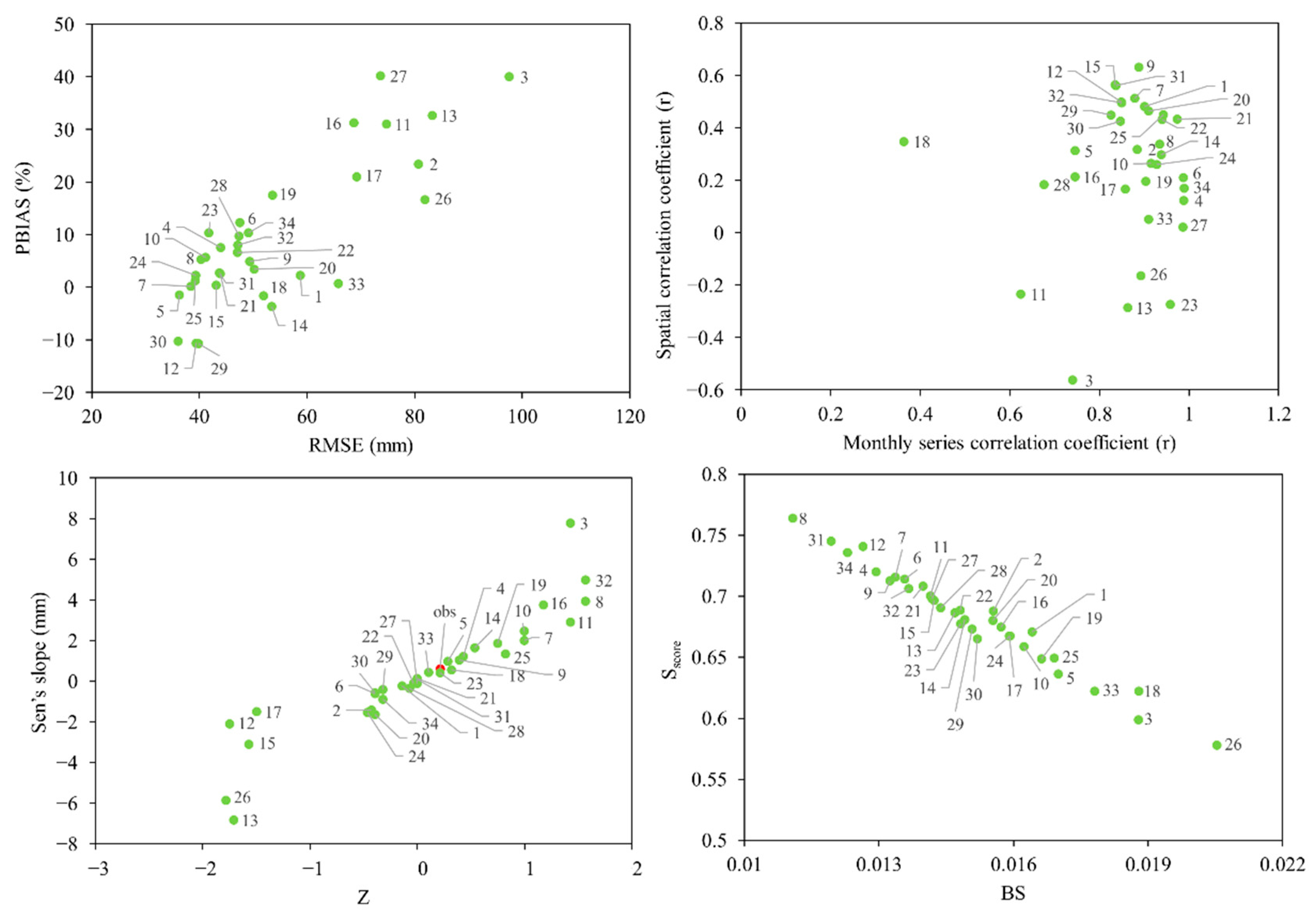
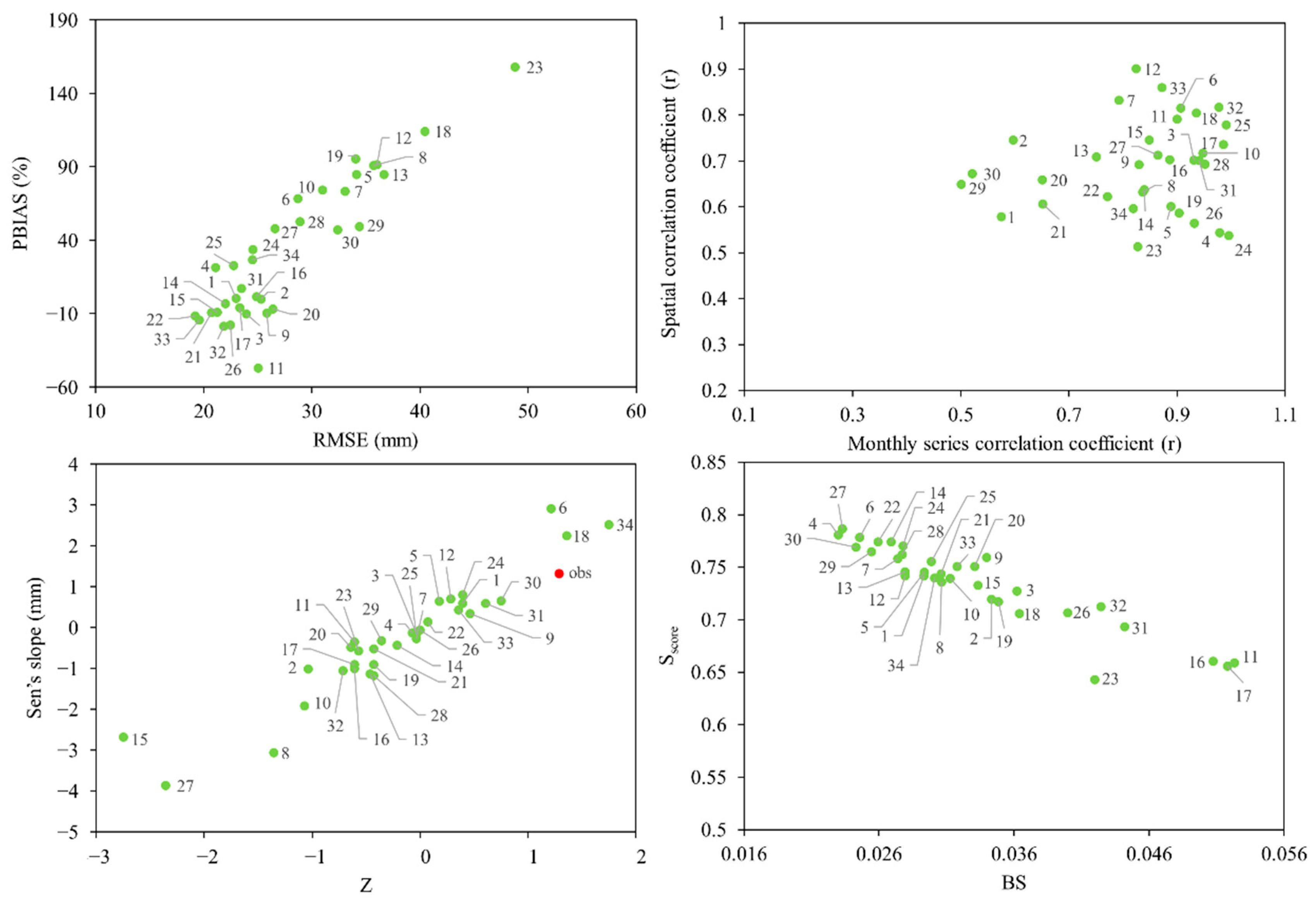
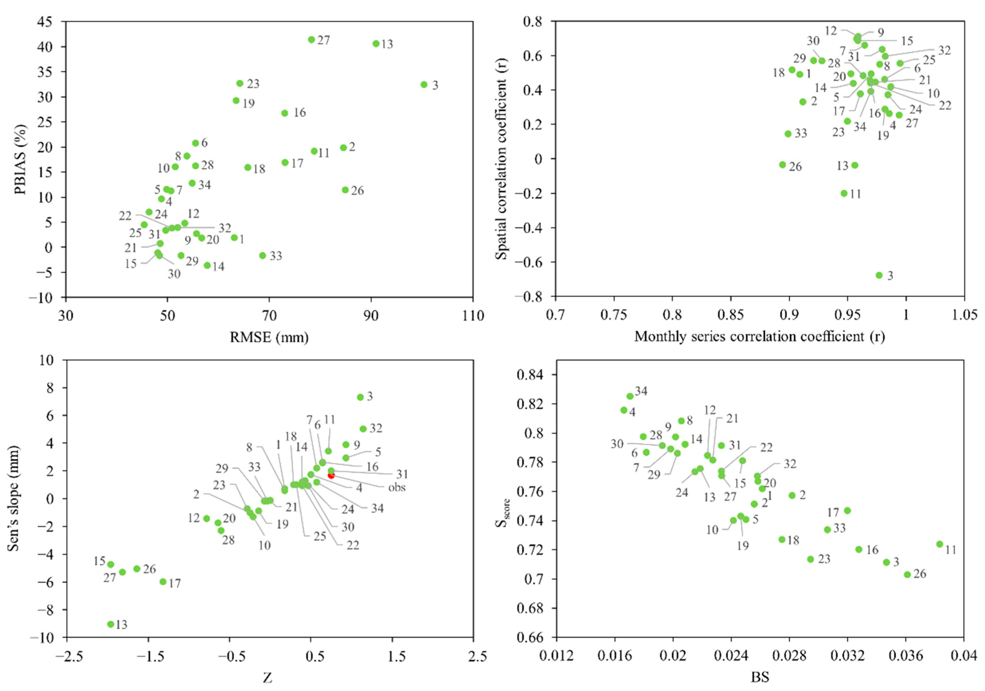
The statistics of the criteria for precipitation concerning the observation and the GCMs simulation were calculated and are shown in terms of scatter plots for the wet season, dry season, and annual time (Figure 4, Figure 5, and Figure 6, respectively). The RMSE was 36.0–97.5 mm, 19.2– 48.8 mm, and 45.4–100.4 mm for the wet season, dry season, and annual time, respectively, with maximum mean and median values of 61.0 mm and 55.5 mm for the annual time, followed by 53.5 mm and 47.4 mm for the wet season, and the minimum values of 27.7 mm and 25.2 mm for the dry season. MIROC-ESM-CHEM, HadGEM2-ES, and IPSL-CM5A-MR had the smallest RMSE values, whereas BCC-CSM1.1, INMCM4.0, and BCC-CSM1.1 had the largest RMSE values for the wet season, dry season, and the annual time, respectively. The PBIAS was −10.7–40.2%, −46.9–158.0%, and −3.6–41.4% for the wet season, dry season, and annual time, respectively, with positive mean and median values for the three time periods of 9.2% and 5.5%, 31.8% and 22.1%, and 12.6% and 11.3%, respectively. In the same respective periods, 28, 21, and 29 (approximately 82.4%, 61.8%, and 85.3%, respectively) of the 34 GCMs had positive PBIAS values, indicating that most of the GCMs overestimated the observation for the wet season and the annual time and a small majority of the GCMs overestimated the observation for the dry season. CESM1(CAM5), ACCESS1.3, and HadGEM2-CC had the lowest absolute PBIAS values at 0.2%, 0.003%, and 0.8%, respectively, for the wet season, dry season, and annual time, indicating good simulation of the observed precipitation. However, MIROC4h, INMCM4.0, and MIROC4h had the highest PBIAS values for the wet season, dry season, and annual time, at 40.2%, 158.0%, and 41.4%, respectively, which represented poor simulation of the observed precipitation.

The monthly series r was obviously high in the annual time and lower for the wet and dry seasons, with mean absolute values of 0.96, 0.86, and 0.84, respectively. Moreover, no obvious difference was noted among GCMs for the annual time due to the absolute r values range of 0.89 to 0.99, indicating that GCMs had good ability in simulating the time series characteristics of precipitation for the annual time. Of the 34 GCMs, 28 and 25, or approximately 82.4% and 73.5%, had relatively higher absolute r values higher than 0.8 for the wet and dry seasons, indicating that GCMs represented a relatively better ability in reproducing the time series characteristics of precipitation for the dry season compared to those for the wet season. NorESM1-M, IPSL-CM5A-LR, and IPSL-CM5A-LR had the highest absolute r values for the wet season, dry season, and annual time, at 0.99, 0.99, and 0.99, respectively, but showed the lowest values for GISS-E2-H, MIROC-ESM, and IPSL-CM5B-LR, at 0.36, 0.50, and 0.89, respectively. The spatial correlation r for the dry season was obviously higher than that for the annual time and the wet season, with mean absolute values of 0.69, 0.44, and 0.34, respectively. Of the 34 GCMs, all had an absolute r value higher than 0.5 for the dry season, whereas 5 and 12 of the GCMs, or approximately 14.7% and 35.3%, had absolute r values higher than 0.5 for the wet season and the annual time, respectively. This phenomenon was also detected in a monsoon region that exhibited low spatial correlation for the wet season [12]. CMCC-CMS, EC-EARTH, and EC-EARTH had the highest absolute r values for the wet season, the dry season, and the annual time, at 0.63, 0.90, and 0.71, respectively, whereas the lowest were shown by MIROC4h, INMCM4.0, and IPSL-CM5B-LR, at 0.02, 0.51, and 0.03, respectively.

The observed precipitation showed positive trends for the wet season, the dry season, and the annual time, with a Z statistic of 0.21, 1.28, and 0.75, and a Sen’s slope of 0.61 mm/year, 1.32 mm/year, and 1.71 mm/year, respectively, without showing the trend at the 0.05 or 0.01 significance level. Of the 34 GCMs, 16, 12, and 19 were able to reproduce the positive trend of observed precipitation for the wet season, the dry season, and the annual time. INMCM4.0, GISS-E2-H, and MPI-ESM-LR showed the smallest absolute error of the Z statistic compared to the observation, with 0, 0.07, and 0, respectively, whereas IPSL-CM5B-LR, GFDL-CM3, and GFDL-CM3(FGOALS-g2) showed the largest absolute error at 2.0, 4.0, and 2.7 (2.7), respectively. GISS-E2-H, IPSL-CM5A-LR, and BNU-ESM showed the smallest absolute error of the Sen’s slope compared to the observation, with 0.06, 0.51, and 0.02, respectively, whereas FGOALS-g2, MIROC4h, and FGOALS-g2 showed the largest absolute error at 7.44, 5.19, and 10.73, respectively.

The BS was 0.011–0.021, 0.023–0.052, and 0.017–0.038 for the wet season, dry season, and annual time, respectively, with maximum mean and median values of 0.033 and 0.031 for the dry season, followed by 0.025 and 0.024 for the annual time, and minimum values of 0.015 and 0.014 for the wet season. The range ability was small for the wet season and the annual time and relatively large for the dry season. CESM1(WACCM), BNU-ESM, and BNU-ESM had the smallest BS values, whereas IPSL-CM5B-LR, CSIRO-Mk3.6.0, and CSIRO-Mk3.6.0 had the largest BS values for the wet season, dry season, and the annual time, respectively. The S_score was 0.578–0.764, 0.643–0.787, and 0.703–0.825 for the wet season, dry season, and annual time, respectively, with maximum mean and median values of 0.766 and 0.772 for the annual time, followed by 0.735 and 0.743 for the dry season, and minimum values of 0.682 and 0.684 for the wet season. IPSL-CM5B-LR, INMCM4.0, and IPSL-CM5B-LR had the smallest S_score values, whereas CESM1(WACCM), MIROC4h, and NorESM1-M had the largest S_score values for the wet season, dry season, and annual time, respectively. All of the S_score values of the GCMs were more than 0.5, and of the 34, 32 (approximately 94.1%), 34 (100%), and 34 (100%) GCMs were more than 0.6 for the wet season, dry season, and annual time, respectively. This indicated that most of the GCMs had good ability in reproducing the characteristics of the probability distribution of the observed precipitation.

3.3. Comparison of Ranking Scores of the GCMs’ Performances by a Single Criterion

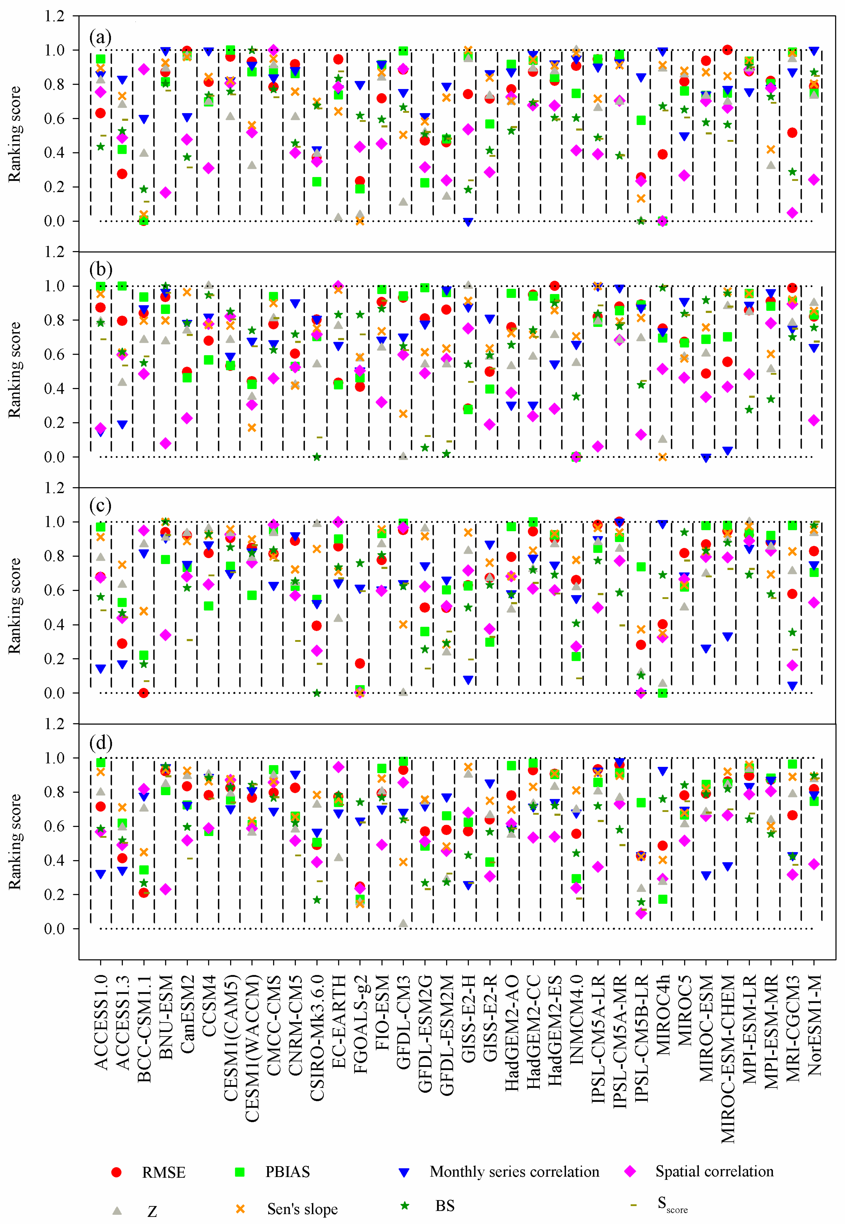
For the different criteria at the same time period, a GCM may have performed well for one criterion but poor for another (Figure 7). For example, MIROC-ESM-CHEM had the highest-ranking score of 1 based on the RMSE criterion for the wet season, but a low-ranking score of 0.467 for the S_score. Although CESM1(WACCM) had the highest-ranking scores, both 1, for the BS and S_score, it had a low-ranking score of 0.321 for the Z for the wet season. The same characteristics were also found for the dry season and the annual time. Moreover, for the same criterion at different time periods, a GCM may have performed well for one time period but poor for another period or for an overall result (Figure 7). For example, ACCESS1.3 had the highest-ranking score of 1 by the PBIAS criterion for the dry season, but low-ranking scores of 0.419 and 0.529 for the wet season and the annual time, respectively. Additionally, a GCM may not have performed the best for one period, two periods, or three periods, but showed the best performance for the overall result (Figure 7). For example, MPI-ESM-LR did not obtain the highest-ranking scores by the Sen’s slope criterion for the three time periods, but had the highest-ranking score of Sen’s slope for the overall result. This indicated that the results of GCMs’ performances relied mainly on the assessment of the criterion, and the GCMs’ performances varied as the criterion changed. Thus, it is essential to comprehensively assess GCMs by using a multiple criteria method, rather than a single criterion method.

3.4. Overall Ranking Scores of the GCMs’ Performances by Multiple Criteria

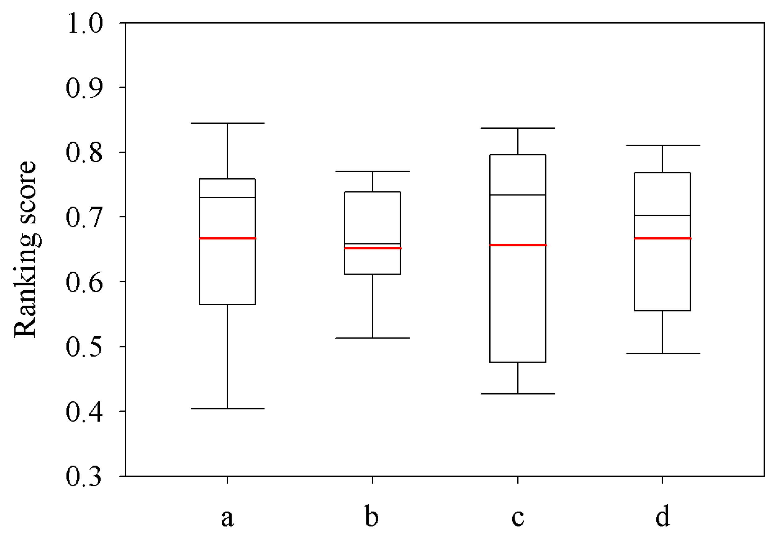
As shown in

Table 2. Ranking scores of the GCMs’ performances for the wet season, dry season, annual time, and overall results over the LMB.

GCMs	ID	Wet	Dry	Annual	Overall
						ACCESS1.0	1	0.753	0.633	0.640	0.667
ACCESS1.3	2	0.546	0.614	0.429	0.505
BCC-CSM1.1	3	0.310	0.740	0.464	0.494
BNU-ESM	4	0.757	0.760	0.814	0.786
CanESM2	5	0.726	0.595	0.743	0.702
CCSM4	6	0.720	0.780	0.762	0.756
CESM1(CAM5)	7	0.842	0.672	0.832	0.795
CESM1(WACCM)	8	0.779	0.468	0.781	0.702
CMCC-CMS	9	0.864	0.735	0.841	0.820
CNRM-CM5	10	0.698	0.613	0.694	0.675
CSIRO-Mk3.6.0	11	0.430	0.622	0.451	0.489
EC-EARTH	12	0.738	0.690	0.779	0.746
FGOALS-g2	13	0.379	0.540	0.248	0.353
FIO-ESM	14	0.738	0.745	0.764	0.753
GFDL-CM3	15	0.747	0.656	0.731	0.716
GFDL-ESM2G	16	0.447	0.622	0.560	0.548
GFDL-ESM2M	17	0.481	0.670	0.476	0.526
GISS-E2-H	18	0.571	0.606	0.547	0.568
GISS-E2-R	19	0.602	0.511	0.569	0.563
HadGEM2-AO	20	0.754	0.621	0.694	0.691
HadGEM2-CC	21	0.847	0.634	0.800	0.770
HadGEM2-ES	22	0.791	0.741	0.785	0.776
INMCM4.0	23	0.763	0.244	0.440	0.472
IPSL-CM5A-LR	24	0.726	0.738	0.804	0.768
IPSL-CM5A-MR	25	0.790	0.821	0.844	0.824
IPSL-CM5B-LR	26	0.331	0.661	0.219	0.358
MIROC4h	27	0.491	0.623	0.424	0.491
MIROC5	28	0.640	0.688	0.701	0.682
MIROC-ESM	29	0.743	0.515	0.737	0.683
MIROC-ESM-CHEM	30	0.745	0.592	0.794	0.731
MPI-ESM-LR	31	0.879	0.733	0.882	0.844
MPI-ESM-MR	32	0.709	0.751	0.807	0.769
MRI-CGCM3	33	0.609	0.853	0.473	0.602
NorESM1-M	34	0.734	0.684	0.791	0.750

, the top five ranking scores of the GCMs over the LMB were MPI-ESM-LR (0.879), CMCC-CMS (0.864), HadGEM2-CC (0.847), CESM1(CAM5) (0.842), and HadGEM2-ES (0.791) for the wet season; MRI-CGCM3 (0.853), IPSL-CM5A-MR (0.821), CCSM4 (0.780), BNU-ESM (0.760), and MPI-ESM-MR (0.751) for the dry season; and MPI-ESM-LR (0.882), IPSL-CM5A-MR (0.844), CMCC-CMS (0.841), CESM1(CAM5) (0.832), and BNU-ESM (0.814) for the annual time. Additionally, the top five overall ranking scores of the GCMs over the LMB were MPI-ESM-LR (0.844), IPSL-CM5A-MR (0.824), CMCC-CMS (0.820), CESM1(CAM5) (0.795), and BNU-ESM (0.786). Figure 8 shows that the mean ranking scores of the GCMs of the wet season were slightly higher than those of the annual time, the dry season, and the overall results. However, the range ability of ranking scores of the GCMs showed the smallest for the dry season compared to the others. This indicated that the GCMs performed relatively better for the wet season, and the seasonal performance was comparatively different.

3.5. Sensitivity Analysis of Ranking Scores of the GCMs’ Performances

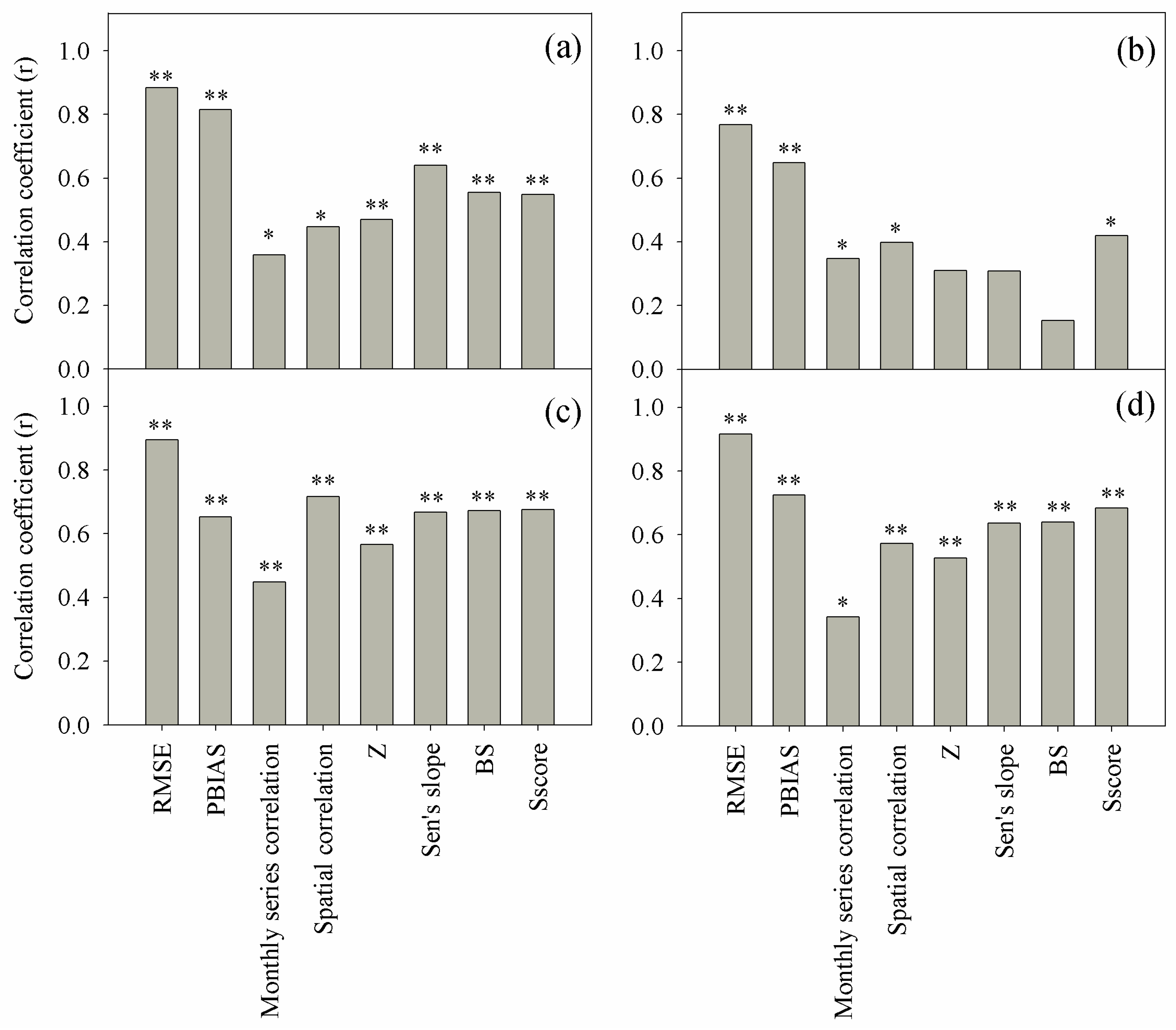
As shown in Figure 9, except Z, Sen’s slope, and BS showing no significant correlations between ranking scores of the GCMs obtained from multiple criteria and ranking scores of the GCMs obtained from a single criterion over the LMB for the dry season, all the criteria showed significant correlations (p < 0.05 or 0.01) for the wet season, the annual time, and the overall results. The RMSE and PBIAS showed relatively high r values compared to other criteria, whereas the monthly series correlation showed the lowest r for the wet season, the annual time, and the overall results. The results indicated that the criteria were robust criteria for assessing performance of the GCMs. However, there existed different robust criteria for assessing performance of the GCMs at a seasonal scale.

3.6. Atmospheric Circulation

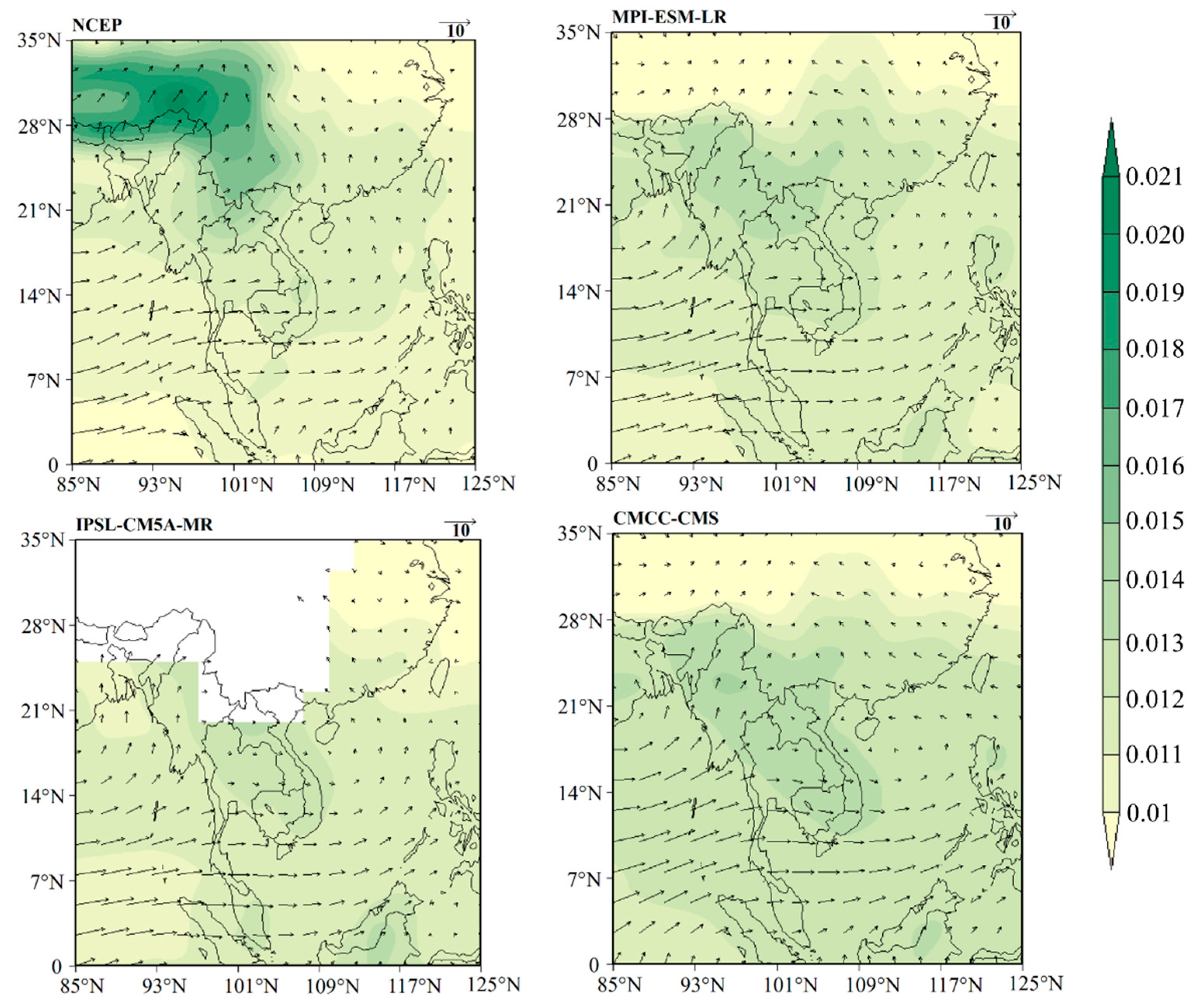
As shown in Figure 10 and Figure 11, the three best-ranked GCMs (overall results) generally represented similar distributions of specific humidity and wind compared to the NCEP reanalysis for the wet season and the dry season, suggesting that a good representation of the regional circulation pattern could also indicate efficiency of model performance [46]. However, the distributions were entirely different between the wet season and the dry season. For the wet season, specific humidity was higher than the dry season, and the prevailing wind direction was dominated by a westerly wind, with large amounts of moisture brought to the LMB from the Bay of Bengal. For the dry season, the prevailing wind direction showed an easterly wind originating from inland, which was characterized by dry weather over the LMB. This indicated that precipitation amounts for the wet season were much higher compared to the dry season, and therefore it was also more likely that the GCMs had larger absolute errors for the wet season compared to the dry season over the LMB.

4. Discussion

In this paper, we obtained the better-performing GCMs in reproducing the observed precipitation over the LMB for the wet season, the dry season, the annual time, and the overall results. A previous study by Sperber et al. 2013 [9] showed that the IPSL-CM5A-LR and IPSL-CM5A-MR models were top performers in representing the interannual variability of the Indian monsoon. Research by Kadel et al. 2018 [23] showed that ACCESS1.0, CNRM-CM5, EC-EARTH, and HadGEM2-ES were the four best models for precipitation simulation in the central Himalayas. Additionally, a study by Hasson et al. 2016 [13] showed that CCSM4, GFDLCM3, MIROC-ESM-CHEM, MIROC-ESM, MIROC5, and NorESM1-M simulated mostly a realistic active duration of the monsoon due to a rapid fractional accumulation (RFA) slope similar to that of the observations in the Mekong River Basin. In our study, we highlighted similarly good performances from HadGEM2-ES, CCSM4, and IPSL-CM5A-MR over the LMB, which is part of the Asian monsoon region, and part of the Mekong River Basin, which are both affected by the southwest monsoon. However, our results showed differences from the above studies, which indicated that it is significant to assess GCM performance not only at a large scale, but also at a regional scale: A river basin such as the LMB should especially be taken into important consideration due to its special geographical position and climatic characteristics, as well as its significant effects [30,31].

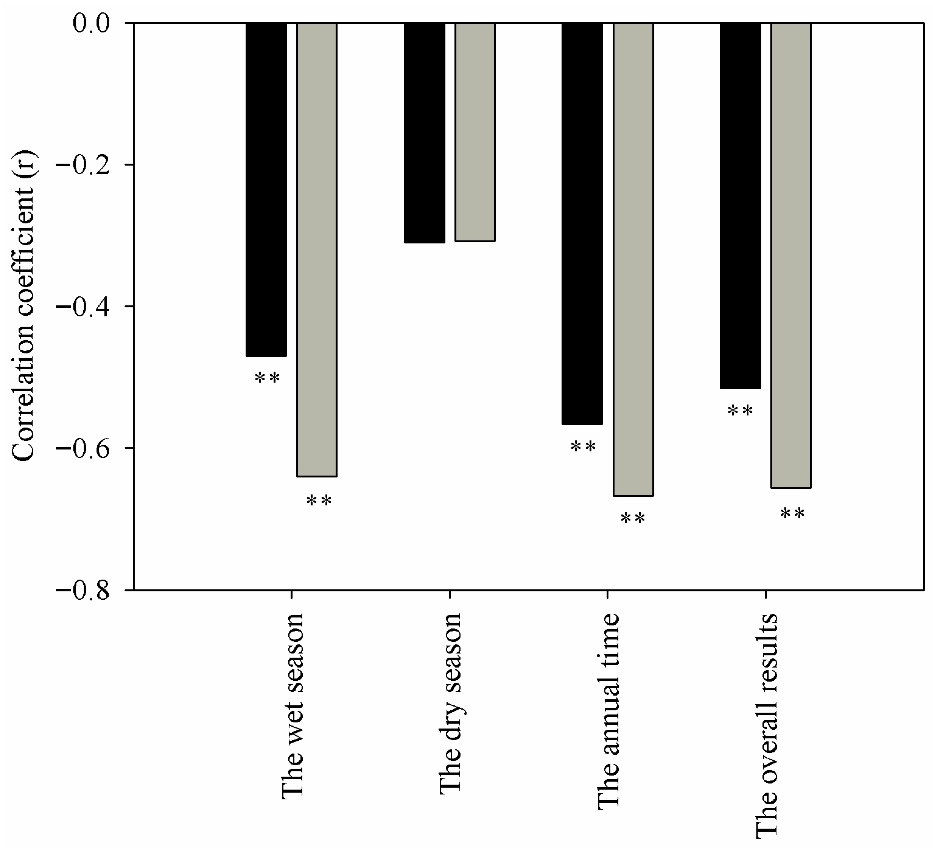
The results showed that there existed different abilities in reproducing the observed precipitation, such as the different statistics of criteria and ranking scores of the GCMs, especially for the differences at the seasonal scale. Actually, this may have really reflected the ability of reproducing the South Asian summer monsoon, which can be caused by issues related to large-scale atmospheric circulations and underrepresentation of real orography [13]. Moreover, previous studies have shown that atmospheric circulation was a good indicator for explaining the discrepancies of simulations by GCMs [33,47]. Thus, how well the GCMs performed in reproducing atmospheric circulation aids in understanding the performance of the GCMs in precipitation simulation. More than 50% of the GCMs failed to reproduce the positive trend of the observed precipitation for the wet season and the dry season (approximately 52.9% and 64.7%, respectively), and approximately 44.1% of the GCMs failed to reproduce positive trend for the annual time over the LMB. Other studies of southeastern Australia by Fu et al. 2013 [45] and the Western Himalayan region by Meher et al. 2017 [12] reported that trend analysis was not a robust criterion for assessing the performance of GCMs. However, our results showed that the Z and Sen’s slope were robust criteria for assessing the performance of GCMs except for the dry season, indicating that the trend analysis method could be used as a robust criterion for assessing GCM performance over the LMB. Nevertheless, in fact more than 50% of the GCMs failed to reproduce a positive trend for the wet season and the dry season. This can be attributed to the parameter we used for assessment and that the ranking scores of the Z and Sen’s slope were based on absolute error between precipitation of the observation and precipitation of the GCM simulation. As shown in Figure 12, the absolute errors of the Z and Sen’s slope showed a significant correlation at the 0.01 significance level with ranking scores of the GCMs except for the dry season, which showed the same significant correlation at the 0.01 significance level between the ranking scores of the GCMs obtained by the Z and Sen’s slope and the ranking scores obtained by multiple criteria (Figure 9 and Figure 12). These results indicated that although the trend analysis method was a robust criterion for assessing the GCMs’ performances except for the dry season, it did not mean a high ability to reproduce the observed precipitation trend. Furthermore, using multiple criteria to assess GCM performance was superior to a single criterion method.

A score-based method proved to be applicable for assessing GCM performance [39,45]. In this paper, we used APHRODITE precipitation data as the observations based on an improved score-based method to provide more detailed assessment results of the GCMs under the three time periods over the LMB. The results provided useful information for further studies related to multimodel ensemble method application and future climate change over the LMB and for monsoon regions that have geographic and climatic features similar to those of the LMB. Although the APHRODITE precipitation data have high resolution and have proven to be a better-gridded precipitation product for the Mekong River Basin, it is important to make a comparison to other gridded precipitation products, such as precipitation data from the Climate Research Unit (CRU) [48], the Global Precipitation Climatology Project (GPCP) [49], and others. In addition, because of the release of a new generation of climate models (CMIP6) in the near future, the improved score-based method can be used for assessing their performance in climatic variables simulation and for their comparison with CMIP5 GCMs.

5. Conclusions

This study focused mainly on the assessment of the performance of 34 CMIP5 GCMs in simulating observed precipitation over the LMB. The performance was assessed through RMSE, PBIAS, monthly series correlations, spatial correlations, Z, Sen’s slope, BS, and S_score under three periods including the wet season, the dry season, and annual time. The overall ranking scores were obtained for GCM performance over the LMB. The main results of this study are presented in the following points.

Precipitation in the observations were 1430.7 mm, 1213.8 mm, 216.9 mm for the mean annual, the mean wet season, and the mean dry season, whereas the precipitation of the GCMs ranged from 1379.7 mm to 2022.9 mm, 1083.5 mm to 1701.9 mm, and 115.1 mm to 559.6 mm, with higher precipitation than the observation at GCM numbers of 29, 21, and 29 (approximately 85.3%, 61.8%, and 85.3%, respectively). This indicated that the GCMs tended to overestimate precipitation compared to the observation, especially for the wet season.

The GCMs showed good ability in reproducing the time series characteristics of precipitation for the annual period compared to those for the wet and dry seasons, and the GCMs obviously reproduced the spatial characteristics of precipitation for the dry season better than those for the annual time and the wet season. More than 50% of the GCMs failed to reproduce the positive trend of the observed precipitation for the wet season and the dry season (approximately 52.9% and 64.7%, respectively), and approximately 44.1% of the GCMs failed to reproduce the positive trend for the annual time over the LMB. However, most showed good ability in reproducing the characteristics of the probability distribution function of the observed precipitation.

The results showed that a GCM may perform well for one criterion but poorly for another criterion at the same period. Moreover, for the same criterion at different periods, a GCM may perform well for one time period but poorly for another period or for the overall result. For example, MIROC-ESM-CHEM had the highest-ranking score of 1 based on the RMSE criterion for the wet season, but a low-ranking score of 0.467 for the S_score. Moreover, for the same criterion at different time periods, ACCESS1.3 had the highest-ranking score of 1 by the PBIAS criterion for the dry season, but low-ranking scores of 0.419 and 0.529 for the wet season and the annual time, respectively. This indicated that the results of GCM performances relied mainly on the assessment of the criterion, and GCM performance varied as the criterion changed. Thus, it is essential to comprehensively assess the GCMs by using a multiple criteria method, rather than a single criterion method.

Based on the ranking scores of the GCMs, the top five ranking scores of the GCMs over the LMB were MPI-ESM-LR (0.879), CMCC-CMS (0.864), HadGEM2-CC (0.847), CESM1(CAM5) (0.842), and HadGEM2-ES (0.791) for the wet season; MRI-CGCM3 (0.853), IPSL-CM5A-MR (0.821), CCSM4 (0.780), BNU-ESM (0.760), and MPI-ESM-MR (0.751) for the dry season; and MPI-ESM-LR (0.882), IPSL-CM5A-MR (0.844), CMCC-CMS (0.841), CESM1(CAM5) (0.832), and BNU-ESM (0.814) for the annual time. Additionally, the top five overall ranking scores of the GCMs over the LMB were MPI-ESM-LR (0.844), IPSL-CM5A-MR (0.824), CMCC-CMS (0.820), CESM1(CAM5) (0.795), and BNU-ESM (0.786). This indicated that it should be realized that the well-performing GCMs changed as the time periods changed.

Assessing performances of the GCMs in reproducing observed precipitation is significant for projecting future climate change. The results of this study can provide useful information for further study related to multimodel ensemble methods application and future climate change over the LMB and for monsoon regions that have geographic and climatic features similar to those of the LMB.

References

- Busuioc, A.; Chen, D.; Hellström, C. Performance of statistical downscaling models in GCM validation and regional climate change estimates: Application for Swedish precipitation. Int. J. Climatol. 2001, 21, 557–578. [Google Scholar] [CrossRef]
- Wilk, J.; Andersson, L.; Plermkamon, V. Hydrological impacts of forest conversion to agriculture in a large river basin in northeast Thailand. Hydrol. Process. 2001, 15, 2729–2748. [Google Scholar] [CrossRef]
- Alavian, V.; Qaddumi, H.M.; Dickson, E.; Diez, S.M.; Danilenko, A.D.; Hirji, R.F.; Puz, G.; Pizarro, C.; Jacobsen, M.; Blankespoor, B. Water and Climate Change: Understanding the Risks and Making Climate-Smart Investment Decisions. Washington, D.C, the World Bank. 2009. Available online: http://citeseerx.ist.psu.edu/viewdoc/download?doi=10.1.1.734.5926&rep=rep1&type=pdf (accessed on 10 September 2018).
- IPCC Secretariat. Climate Change and Water: Technical Paper of The Intergovernmental Panel on Climate Change; Bates, B.C., Kundzewicz, Z.W., Wu, S., Palutikof, J.P., Eds.; IPCC: Geneva, Switzerland, 2008. [Google Scholar]
- Eastham, J.; Mpelasoka, F.; Mainuddin, M.; Ticehurst, C.; Dyce, P.; Hodgson, G.; Ali, R.; Kirby, M. Mekong River Basin Water Resources Assessment: Impacts of climate change, CSIRO: Water for a Healthy Country National Research Flagship, 2008. Available online: http://www.clw.csiro.au/publications/waterforahealthycountry/2008/wfhc-MekongWaterResourcesAssessment.pdf (accessed on 20 September 2018).
- 2030 WRG (2030 Water Resources Group). Charting Our Water Future: Economic Frameworks to Inform Decision-Making; McKinsey & Company: New York, NY, USA, 2009. [Google Scholar]
- Xu, Y.; Xu, C.H.; Gao, X.J.; Luo, Y. Projected changes in temperature and precipitation extremes over the Yangtze River basin of China in the 21st century. Quat. Int. 2009, 208, 44–52. [Google Scholar] [CrossRef]
- Ramesh, K.V.; Goswami, P. Assessing reliability of regional climate projections: The case of Indian monsoon. Sci. Rep. 2014, 4, 4071. [Google Scholar] [CrossRef] [PubMed]
- Sperber, K.R.; Annamalai, H.; Kang, I.S.; Kitoh, A.; Moise, A.; Turner, A.; Wang, B.; Zhou, T. The Asian summer monsoon: An intercomparison of CMIP5 vs. CMIP3 simulations of the late 20th century. Clim. Dynam. 2013, 41, 2711–2744. [Google Scholar] [CrossRef]
- Sillmann, J.; Kharin, V.V.; Zhang, X.; Zwiers, F.W.; Bronaugh, D. Climate extremes indices in the CMIP5 multimodel ensemble: Part 1. Model evaluation in the present climate. J. Geophys. Res.-Atmos. 2013, 118, 1716–1733. [Google Scholar] [CrossRef] [Green Version]
- Sun, Q.H.; Miao, C.Y.; Duan, Q.Y. Comparative analysis of CMIP3 and CMIP5 global climate models for simulating the daily mean, maximum, and minimum temperatures and daily precipitation over China. J. Geophys. Res.-Atmos. 2015, 120, 4806–4824. [Google Scholar] [CrossRef] [Green Version]
- Meher, J.K.; Das, L.; Akhter, J.; Benestad, R.E.; Mezghani, A. Performance of CMIP3 and CMIP5 GCMs to Simulate Observed Rainfall Characteristics over the Western Himalayan Region. J. Clim. 2017, 30, 7777–7799. [Google Scholar] [CrossRef]
- Hasson, S.; Pascale, S.; Lucarini, S.; Böhner, J. Seasonal cycle of precipitation over major river basins in South and Southeast Asia: A review of the CMIP5 climate models data for present climate and future climate projections. Atmos. Res. 2016, 180, 42–63. [Google Scholar] [CrossRef] [Green Version]
- Kumar, S.; Merwade, V.; Kinter III, J.L.; Niyogi, D. Evaluation of Temperature and Precipitation Trends and Long-Term Persistence in CMIP5 Twentieth-Century Climate Simulations. J. Clim. 2013, 26, 4168–4185. [Google Scholar] [CrossRef]
- Kumar, D.; Kodra, E.; Ganguly, A.R. Regional and seasonal intercomparison of CMIP3 and CMIP5 climate model ensembles for temperature and precipitation. Clim. Dynam. 2014, 43, 2491–2518. [Google Scholar] [CrossRef]
- Koutroulis, A.G.; Grillakis, M.G.; Tsanis, I.K.; Papadimitriou, L. Evaluation of precipitation and temperature simulation performance of the CMIP3 and CMIP5 historical experiments. Clim. Dynam. 2016, 47, 1881–1898. [Google Scholar] [CrossRef]
- Nguyen, P.; Thorstensen, A.; Sorooshian, S.; Zhu, Q.; Tran, H.; Ashouri, H.; Miao, C.Y.; Hsu, K.L.; Gao, X.G. Evaluation of CMIP5 model precipitation using PERSIANN-CDR. J. Hydrometeorol. 2017, 18, 2313–2330. [Google Scholar] [CrossRef]
- Yoo, C.; Cho, E. Comparison of GCM precipitation predictions with their RMSEs and pattern correlation coefficients. Water. 2018, 10, 28. [Google Scholar]
- Zhou, B.T.; Wen, Q.Z.H.; Xu, Y.; Song, L.C.; Zhang, X.B. Projected changes in temperature and precipitation extremes in China by the CMIP5 multimodel ensembles. J. Clim. 2014, 27, 6591–6611. [Google Scholar] [CrossRef]
- Almazroui, M.; Islam, M.N.; Saeed, S.; Alkhalaf, A.K.; Dambul, R. Assessment of uncertainties in projected temperature and precipitation over the Arabian Peninsula using three categories of CMIP5 multimodel ensembles. Earth. Syst. Environ. 2017. [Google Scholar] [CrossRef]
- Abbasian, M.; Moghim, S.; Abrishamchi, A. Performance of the general circulation models in simulating temperature and precipitation over Iran. Theor. Appl. Climatol. 2018. [Google Scholar] [CrossRef]
- Hussain, M.; Yusof, K.W.; Mustafa, M.R.U.; Mahmood, R.; Jia, S.F. Evaluation of CMIP5 models for projection of future precipitation change in Bornean tropical rainforests. Theor. Appl. Climatol. 2017, 134, 1–18. [Google Scholar] [CrossRef]
- Kadel, I.; Yamazaki, T.; Iwasaki, T.; Abdillah, M.R. Projection of future monsoon precipitation over the central Himalayas by CMIP5 models under warming scenarios. Clim. Res. 2018, 75, l–21. [Google Scholar] [CrossRef]
- Lovino, M.A.; Müller, O.V.; Berbery, E.H.; Müller, G.V. Evaluation of CMIP5 retrospective simulations of temperature and precipitation in northeastern Argentina. Int. J. Climatol. 2018, 38, e1158–e1175. [Google Scholar] [CrossRef] [Green Version]
- Miao, C.Y.; Duan, Q.Y.; Sun, Q.H.; Huang, Y.; Kong, D.X.; Yang, T.T.; Ye, A.Z.; Di, Z.H.; Gong, W. Assessment of CMIP5 climate models and projected temperature changes over Northern Eurasia. Environ. Res. Lett. 2014, 9, 055007. [Google Scholar] [CrossRef] [Green Version]
- Penalba, O.; Rivera, J. Regional aspects of future precipitation and meteorological drought characteristics over southern South America projected by a CMIP5 multi-model ensemble. Int. J. Climatol. 2016, 36, 974–986. [Google Scholar] [CrossRef]
- IPCC (Intergovernmental Panel on Climate Change), Climate Change 2014: Impacts, Adaptation, and Vulnerability. Working Group II Contribution to the Fifth Assessment Report of the Intergovernmental Panel on Climate Change, Cambridge/New York, Cambridge University Press. 2014. Available online: https://www.ipcc.ch/site/assets/uploads/2018/02/WGIIAR5-PartA_FINAL.pdf (accessed on 10 August 2018).
- Jacobs, J.W. The mekong river commission: Transboundary water resources planning and regional security. Geogr. J. 2002, 168, 354–364. [Google Scholar] [CrossRef]
- MRC: State of the Basin Report. Mekong River Commission, Vientiane, Lao PDR. 2010. Available online: http://www.mrcmekong.org/assets/Publications/basin-reports/MRC-SOB-report-2010full-report.pdf (accessed on 15 August 2018).
- Thilakarathne, M.; Sridhar, V. Characterization of future drought conditions in the Lower Mekong River Basin. Weather Clim. Extrem. 2017, 17, 47–58. [Google Scholar] [CrossRef]
- Trisurat, Y.; Aekakkararungroj, A.; Ma, H.; Johnston, J.M. Basin-wide impacts of climate change on ecosystem services in the Lower Mekong Basin. Ecol. Res. 2018, 33, 73–86. [Google Scholar] [CrossRef] [PubMed]
- Hirota, N.; Takayabu, Y.N. Reproducibility of precipitation distribution over the tropical oceans in CMIP5 multi-climate models compared to CMIP3. Clim. Dynam. 2013, 41, 2909–2920. [Google Scholar] [CrossRef] [Green Version]
- Zazulie, N.; Rusticucci, M.; Raga, G.B. Regional climate of the subtropical central Andes using high-resolution CMIP5 models—Part I: Past performance (1980–2005). Clim. Dynam. 2017, 49, 3937–3957. [Google Scholar] [CrossRef]
- Lutz, A.; Terink, W.; Droogers, P.; Immerzeel, W.; Piman, T. Development of Baseline Climate Data Set and Trend Analysis in the Mekong Basin. Wageningen, The Netherlands. 2014, pp. 1–127. Available online: https://www.futurewater.eu/wp-content/uploads/2014/04/MRC_baseline_climate_report_v14.pdf (accessed on 2 September 2018).
- Yatagai, A.; Kamiguchi, K.; Arakawa, O.; Hamada, A.; Yasutomi, N.; Kitoh, A. APHRODITE: Constructing a long-term daily gridded precipitation dataset for Asia based on a dense network of rain gauges. Bull. Am. Meteorol. Soc. 2012, 93, 1401–1415. [Google Scholar] [CrossRef]
- MRC: Adaptation to climate change in the countries of the Lower Mekong Basin. Regional Synthesis Report. Mekong River Commission, Vientiane, Lao PDR. 2009. Available online: http://www.mrcmekong.org/assets/Publications/report-management-develop/MRC-IM-No1-Adaptation-to-climate-change-in-LMB.pdf (accessed on 15 September 2018).
- MRC: Planning atlas of the Lower Mekong River Basin. Basin Development Plan Programme. Mekong River Commission, Vientiane, Lao PDR. 2011. Available online: http://www.mrcmekong.org/assets/Publications/basin-reports/BDP-Atlas-Final-2011.pdf (accessed on 1 October 2018).
- Taylor, K.E.; Stouffer, R.J.; Meehl, G.A. An overview of CMIP5 and the experiment design. Bull. Am. Meteorol. Soc. 2012, 93, 485–498. [Google Scholar] [CrossRef]
- Liu, Z.F.; Wang, R.; Yao, Z.J. Air temperature and precipitation over the Mongolian Plateau and assessment of CMIP5 climate models. Resour. Sci. 2016, 38, 956–969. (In Chinese) [Google Scholar]
- Hirsch, R.M.; Alexander, R.B.; Smith, R.A. Selection of methods for the detection and estimation of trends in water quality. Water Resour. Res. 1991, 27, 803–813. [Google Scholar] [CrossRef]
- Sen, P.K. Estimates of the regression coefficient based on Kendall’s tau. J. Am. Stat. Assoc. 1968, 63, 1379–1389. [Google Scholar] [CrossRef]
- Hirsch, R.M.; Slack, J.R.; Smith, R.A. Techniques of trend analysis for monthly water quality. Water Resour. Res. 1982, 18, 107–121. [Google Scholar] [CrossRef]
- Brier, G.W. Verification of forecasts expressed in terms of probability. Mon. Weather Rev. 1950, 78, 1–3. [Google Scholar] [CrossRef]
- Perkins, S.E.; Pitman, A.J.; Holbrook, N.J.; McAneney, J. Evaluation of the AR4 climate models’ simulated daily maximum temperature, minimum temperature, and precipitation over Australia using probability density functions. J. Clim. 2007, 20, 4356–4376. [Google Scholar] [CrossRef]
- Fu, G.B.; Liu, Z.F.; Charles, S.P.; Xu, Z.X.; Yao, Z.J. A score-based method for assessing the performance of GCMs: A case study of southeastern Australia. J. Geophys. Res.-Atmos. 2013, 118, 4154–4167. [Google Scholar] [CrossRef] [Green Version]
- Bannister, D.; Herzog, M.; Graf, H.; Hosking, J.S.; Short, C.A. An assessment of recent and future temperature change over the Sichuan Basin, China, Using CMIP5 Climate Models. J. Clim. 2017, 30, 6701–6722. [Google Scholar] [CrossRef]
- Wang, X.; Chen, M.Y.; Wang, C.Z.; Yeh, S.W.; Tan, W. Evaluation of performance of CMIP5 models in simulating the North Pacific Oscillation and El Niño Modoki. Clim. Dynam. 2018, 1–12. [Google Scholar] [CrossRef]
- Harris, I.; Jones, P.D.; Osborn, T.J.; Lister, D.H. Updated high-resolution grids of monthly climatic observations—The CRU TS3.10 Dataset. Int. J. Climatol. 2013, 34, 623–642. [Google Scholar] [CrossRef]
- Schneider, U.; Becker, A.; Finger, P.; Meyer-Christoffer, A.; Ziese, M.; Rudolf, B. GPCC’s new land surface precipitation climatology based on quality-controlled in situ data and its role in quantifying the global water cycle. Theor. Appl. Climatol. 2013, 115, 15–40. [Google Scholar] [CrossRef]
Figure 1.
Location of the Lower Mekong Basin (LMB) and observed stations of the Global Surface Summary of the Day (GSOD), the Global Historical Climatology Network (GHCN), and the 21 selected grids over the LMB (shade of blue).
Figure 2.
Correlation of the Asian Precipitation-Highly Resolved Observational Data Integration Towards Evaluation of Water Resources (APHRODITE) and the observed stations for monthly precipitation over the LMB during the period of 1975–2004.
Figure 3.
Variations in observed precipitation and general circulation model (GCM) simulations in the mean annual cycle during the period 1975–2004 over the LMB.
Figure 4.
Scatter plots of statistics of assessment criteria for the wet season over the LMB.
Figure 5.
Scatter plots of statistics of assessment criteria for the dry season over the LMB.
Figure 6.
Scatter plots of statistics of assessment criteria for the annual time over the LMB.
Figure 7.
Ranking scores of the eight criteria over the LMB: (a), (b), (c), and (d) represent the wet season, dry season, annual time, and the overall results, respectively.
Figure 8.
Box plots of ranking scores (ascending orders) for the performance of GCMs over the LMB: a, b, c, and d represent the wet season, dry season, annual time, and the overall results, respectively. The red and black lines in the box represent the mean value and the median value, respectively. The top and bottom horizontal lines represent the maximum value and the minimum value, respectively. The top and bottom horizontal lines on the borders of the box represent the upper quartile and the lower quartile, respectively.
Figure 9.
Correlation between ranking scores of the GCMs obtained from multiple criteria and ranking scores of the GCMs obtained from a single criterion over the LMB: (a), (b), and (c) represent the time periods of the wet season, the dry season, and the annual time, respectively; (d) represents the correlation between the overall ranking scores and the weight criteria ranking scores; ** represents that correlation was significant at the 0.01 level; * represents that correlation was significant at the 0.05 level.
Figure 10.
Mean monthly specific humidity (shaded) and wind (vector) for the wet season of the period 1975–2004 for the National Centers for Environmental Prediction (NCEP) and the three best-ranked GCMs over the LMB.
Figure 11.
Mean monthly specific humidity (shaded) and wind (vector) for the dry season of the period 1975–2004 for the NCEP and the three best-ranked GCMs over the LMB.
Figure 12.
Correlation between the absolute errors for the statistics and ranking scores of the GCMs. Absolute errors for the statistics were between precipitation of the observation and precipitation of the GCM simulations. The black bar represents the Z; the gray bar represents Sen’s slope; ** represents that correlation was significant at the 0.01 level.