Vortex Cascade Features of Turbulent Flow in Hydro-Turbine Blade Passage with Complex Geometry


Faculty of Civil Engineering and Mechanics, Kunming University of Science and Technology, South Jingming Road, Kunming 650500, China
*
Author to whom correspondence should be addressed.
Water 2018, 10(12), 1859; https://doi.org/10.3390/w10121859
Submission received: 6 November 2018
/
Revised: 9 December 2018
/
Accepted: 12 December 2018
/
Published: 14 December 2018
(This article belongs to the Special Issue Applications of Computational Fluid Dynamics for Marine and Offshore Engineering)
Abstract
:A large-eddy simulation of three-dimensional turbulent flow for a hydro-turbine in the transitional process of decreasing load from rated power to no-load has been implemented by using ANSYS-Fluent in this paper. The survival space occupied by different scale flow structures for the different guide vane opening degrees was well captured. The flow characteristics in the transitional process were obtained. Different forms of the channel vortex were studied. The features of the vortex cascade and dissipation of the turbulent energy in blade passage were analyzed. The results show that the scales of the vortex structures have a large change in the transitional process of rejecting load, and the vortex distributions in the blade passage are significantly distinguished. The survival space of the different scale eddies in the blade passage is closely related to the scales of the vortex. The survival volume ratio of the adjacent scale vortex in the runner is about 1.2–1.6. The turbulent kinetic energy and eddy viscosity increase rapidly along the blade passage with the small-scale eddies going up, which implies that a dissipating path for the energy in the blade passage is formed.
1. Introduction
“Big whorls have little whorls that feed on their velocity, and little whorls have smaller whorls, and so on to viscocity (in the molecular sense)”. This famous poem was composed by Lewis Fry Richardson in 1922 [1], which proposed that turbulent cascades were transferring energy from the large-scale eddies energy-generated down to the small scale eddies energy-dissipated. The Richardson’s cascade description was quantified by Kolmogorov [2], which was constituted to be the most fundamental concept of turbulence theory. After almost 100 years, we are still fighting to have a deep understanding and a complete description even for the simplest case of homogeneous and isotropic turbulence [3]. Cascades have been shown to exist in many systems, in different physical situations (like rotating turbulences [4,5,6]), in geophysical flows (for example the atmosphere acts like a 2D flow at large scale [7,8,9]) and astrophysical flows (such as the atmosphere of Jupiter [10]), and in plasma flows [11]. In recent decades, many theories have been established. Alexakis et al. [12] in 2018 provided a critical summary of historical and recent works from a unified point of view, and presented a classification of all known transfer mechanisms. However, it’s still very difficult to use several or even dozens of deterministic equations to describe huge eddy quantities and complicated interactions between eddies.
The internal turbulent flow in a hydro-turbine is very complex. Operating conditions of hydro-turbine change frequently, constantly several times during one day, or even several times in an hour, in which flow patterns in the hydro-turbine are strongly stirred while being largely in flux. The evolution of the hydrodynamic instabilities gives rise to an eddy cascade [13], which may induce a violent coupling vibration of hydroelectric power generation systems. During the transitional process, it is worthwhile to study dramatic changes in flow and vortex, which possibly makes the hydro-turbine operation unstable and unsafe [14].
A large amount of numerical simulations and experimental measurements have been carried out to investigate the great changes in the flow patterns. Widmer et al. [15] investigated the effects of a rotating stall on “S” shape characteristic curves with a pump-turbine model based on numerical simulations. Trivedi et al. [16] carried out measurements on a scale model of a Francis turbine prototype during an emergency shutdown with a transition state into full load rejection. Hu et al. [17] and Yang et al. [18] presented a study of pressure pulsation of a prototype pump-turbine, including steady state and transient state with pressure data measured in spiral case, draft tube inlet and vaneless space. Fluctuation amplitude was estimated, using the contour lines of pressure fluctuations of a model pump turbine with decreasing load. CFD simulations were carried out to analyze the impacts of flow evolution on the pressure pulsations in the S-shaped region of the model pump-turbine (see Xia et al. [19]), on which the results showed that the reverse flow vortex structures (RFVS) at the runner inlet had regular development and transition patterns while discharge was reduced from the best efficiency point (BEP). However, little research concentrates on flow characteristics in the transitional process compared with steady state, as most works usually focus on pressure fluctuation and vortex belt in draft tube. Vortex cascade is a core issue of the turbulent flow in hydro-turbine passage. Therefore study of features of the vortex cascade in a hydro turbine in transitional cases is the motivation of this paper.
Large Eddy Simulation (LES) is a powerful numerical method. It’s currently the method with the most potential and feasible numerical simulation tool for a complicated turbulent flow, such as a hydraulic machinery flow with a complex geometric space and a high Reynolds number. In the present work, we take a pump-turbine as the object. 3D unsteady simulation with LES in transitional process of decreasing load was carried out by using commercial software ANSYS-Fluent 17.1 (ANSYS, Canonsburg, PA, USA). A vortex was well observed in the space dimension. Our goal is to investigate the flow structures in the blade passage during the transitional process, and to explore vortex cascade features.
2. Numerical Setup
2.1. Computation Domain and Grid
A prototype of a Francis pump-turbine with a runner diameter of D1 = 4.6875 m and 7 blades is taken as the simulating object. For the present study, the water head is H = 200 m, the rated flow of the hydro-turbine is 148 m3/s, and the rated rotation speed of the runner is n = 300 rpm. There is a tongue plate at the nose end of the spiral case. A circular arc guide ring is used to connect the spiral case with the guide vane apparatus. The inlet diameter of the spiral case is 3.131 m, and the height of the guide vane apparatus is B0 = 0.6263 m, the distribution circle diameter of the movable guide vane is D0 = 5.625 m, the rated opening of the guide vanes in rated power is = 23, equivalent to 85% of the max opening. The outlet diameter of the runner is D3 = 3 m. The outlet diameter of the draft tube is 6.2194 m.
The software Pro/Engineer is used to model the computational domains of the hydro-turbine. In order to improve simulation precision, the whole turbine flow passages, from the inlet of the spiral case to the outlet of the draft tube, as shown in Figure 1, are taken as the computational domain, including 19 fixed guide vanes and 20 movable guide vanes. The dimensions of the main sections of the geometry are listed in Table 1.
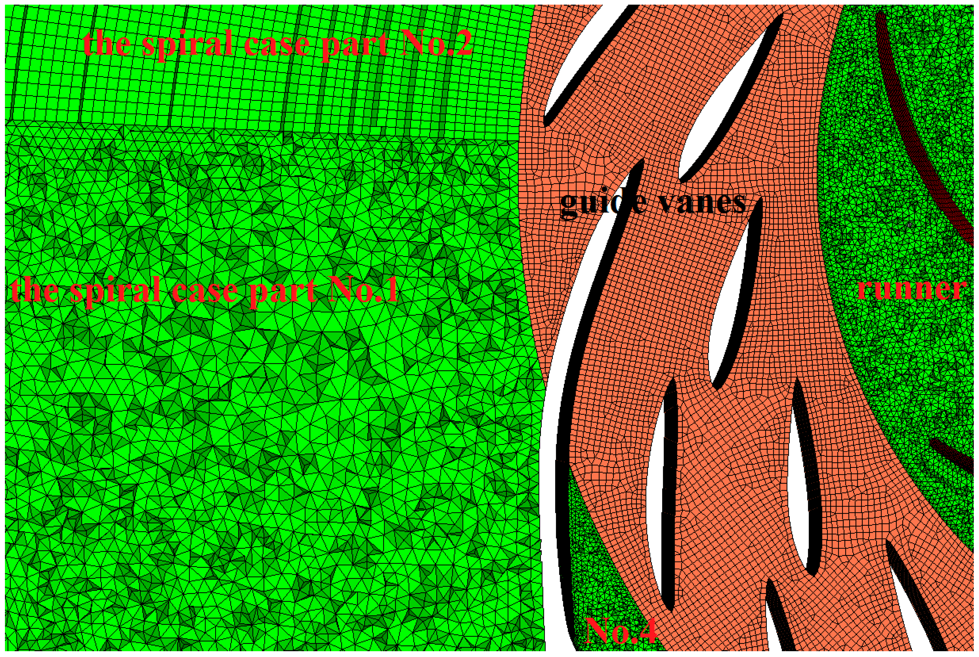
The software HyperMesh has strong adaptability and high customizability in dealing with the mesh geometry. In this paper, the five operation points are selected. In order to avoid the repetitive grid generation, the whole flow passage of the pump-turbine is divided into four components by HyperMesh: spiral case region, guide vane apparatus region, runner region, and draft tube region. Only the component of the guide vane apparatus region are different for the five operation points. All of four components need to be mesh for the first operating point. Only the guide vane apparatus region needs to be mesh for other operating points, because the other area grids are the same as those of the first operating point.
The aim of this paper is to investigate the cascade features of the turbulent flow in a strong 3D blade passage. For such complicated configuration of the computational domain, in order to ensure simulation accuracy and reduce computational cost, the hybrid grid is designed and generated by using HyperMesh according to the flow physics of the different regions and the characteristics of large-scale parallel computing. The interfaces between fluid and solid are dealt as a no-slip boundary surface, and the sliding mesh technology is used to deal with runner-rotating interface. Structured meshes have high quality, while unstructured meshes have a better fit for the complicated geometry. In this paper, the structured meshes are taken as a precedence for consideration. In order to make structured grids cover more calculated regions, the division strategy is implemented according to the passage geometries. The spiral case domain is divided into 5 parts in the circumferential direction of the spiral case body, that is, the spiral case part 1 from the spiral case inlet to section S1, the spiral case part 2 from section S1 to section S7, the spiral case part 3 from section S7 to section S13, the spiral case part 4 from section S13 to section S19, and the spiral case part 5 from section S19 to the large tongue plate. The rotation angle between adjacent sections is 18°. Similarly, the draft tube is divided into 9 parts with different colors, as shown in Figure 1. Considering the influence of the large tongue plate and flow guide ring for the spiral case parts 1 and 5, and the 3D twisted channel for runner, the adaptable tetrahedron unstructured grids are applied to the spiral case parts 1, 5 and the runner. The structured grids are used in the spiral case except for the spiral case parts 1 and 5, the guide vanes mechanism and the draft tube.
Considering that flow changes in diffusion domain of the draft tube are not obvious, the number of the grids in the diffusion domain of the draft tube are reduced to decrease the computing time in the calculation of the whole flow passage. To improve accuracy of the computation, local mesh refinement is carried out in some areas, such as the guide vane apparatus area and the runner area. The maximum grid size in the guide vane apparatus region and the runner is controlled to be less than 15 mm, and ones in the inlet area and the draft tube to be less than 40 mm and 50 mm, respectively. Furthermore, according to our previous research [20], special refinements are applied to near-walled zone of the blades, and the first layer grid is generally set into zone. According to the grid independence verification and the flow pattern analysis [21], the total mesh number of the turbine is about 20 million. The number of the grids in the spiral case region, guide vane apparatus region, runner region and draft tube region is 3,154,197, 909,038, 7,308,144, and 8,314,335, respectively. There is no recommendation to do mesh quality check in the FLUENT. Minimum orthogonal quality and maximum ortho skew are 0.5023, 0.9469, respectively. The local area meshes in the centerplane of the guide vanes are shown in Figure 2.
2.2. Governing Equations
The filtered governing equations of the Newtonian incompressible viscous flow for the hydro-turbine are written as
where stands for the filtered velocity in direction, represents the pressure, stands for the kinetic viscosity, is the subgrid stress (that is, SGS stress).
Furthermore, term in SGS stress is decomposed as:
So, SGS stress is conveyed as
where is Leonard stress, which stands for the interaction between large scale vortices; is Cross stress, stands for the interaction between large scale vortices and small scale vortices; is Reynolds stress, stands for the interaction between small scale vortices.
The presence of the curvature varying blade walls affects the physics of the stresses and inhibits the natural growth of the small-scale vortices. Therefore, compared with flow in a wide and straight passage, energy exchange mechanisms between the resolved and unresolved structures may be significantly altered in a strong 3D passage with complex geometry. To better simulate energy exchange mechanisms in the whole turbine flow passages, the model coefficients keep updating instead of being constant during the computation procedure, as occurs in the classical Smagorinsky model. Therefore, a one-coefficient dynamic SGS model [22,23] is adopted, and the dynamic model is described as
in which
where is Kronecker’s delta, represents the eddy viscosity of fluid, stands for the strain rate tensor, is the grid width in direction.
2.3. Calculation Method and Initial Condition
The finite volume method and the non-staggered grid technique are used for spatial discretization. The second order implicit scheme is used for discrete-time. The SIMPLEC (Semi-Implicit Method for Pressure-Linked Equations-Consistent) scheme is chosen to achieve the coupling solution for pressure and velocity equations. The second order scheme is used for the pressure term, and the second order upwind scheme is used for the momentum term.
The numerical simulations in the transitional process of decreasing load from rated load to no-load are implemented with a constant rotation speed of the runner. The boundary conditions are as follows. A homogenous approach chosen is close to a fully developed velocity distribution applied at the high Reynolds number in the inlet of the spiral case. Considering that the effects of a homogenous approach chosen [24] can be neglected in a numerical simulation for a long inlet section, a homogenous velocity boundary is applied at the inlet of the spiral case, and the velocity is normal to boundary. Outflow is chosen at the outlet of the draft tube. According to actual submergence depth at the outlet, pressure term at operating conditions is set. For the sake of convenience and investigate, the five operation points in the transitional process are selected for unsteady simulation with the principle of equal power. The guide vane opening degree is different for the different operation points. The powers for the five operation points are 100%Pn, 75%Pn, 50%Pn, 25%Pn, 1%Pn, respectively. The computation parameters are listed in Table 2.
In each case, the previous RANS simulation is conducted with the same mesh and Realizable k-ε turbulence model. The results are used as the initial flow field of unsteady calculation. Considering rotation speed and calculation scale, the time that the runner rotates 1.5 is chosen as the time-step, corresponding to 240 time steps per revolution [25]. The convergence criteria of the residuals are 1 × 10⁻³, and the maximum number of iterations per time-step is set to 30. The stable calculation results are selected to analysis. Considering the calculation scale to be large, the simulations are conducted in the PowerCube-S01 cloud cube high performance computing system in Kunming University of Science and Technology for parallel computing. Considering that sometimes the large number of selected CPU cores might not be useful to computation efficiency for different scale parallel computing, 60 CPU cores in node 1 are therefore chosen for parallel computing in this numerical simulation. Each case consumed about 72–96 h, and the total computation time is about 720 h.
3. Results and Analysis
3.1. Transitional Process from Rated Load to No-Load
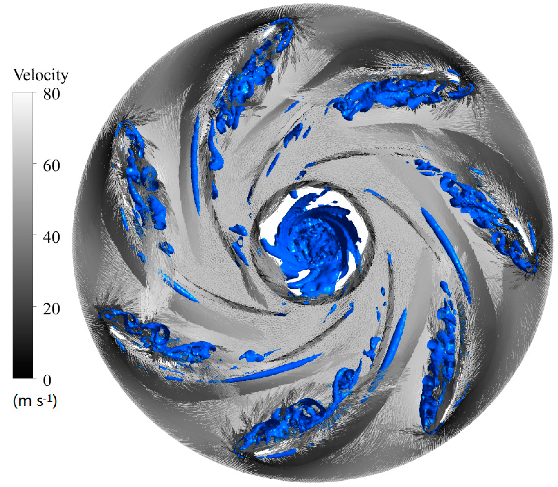
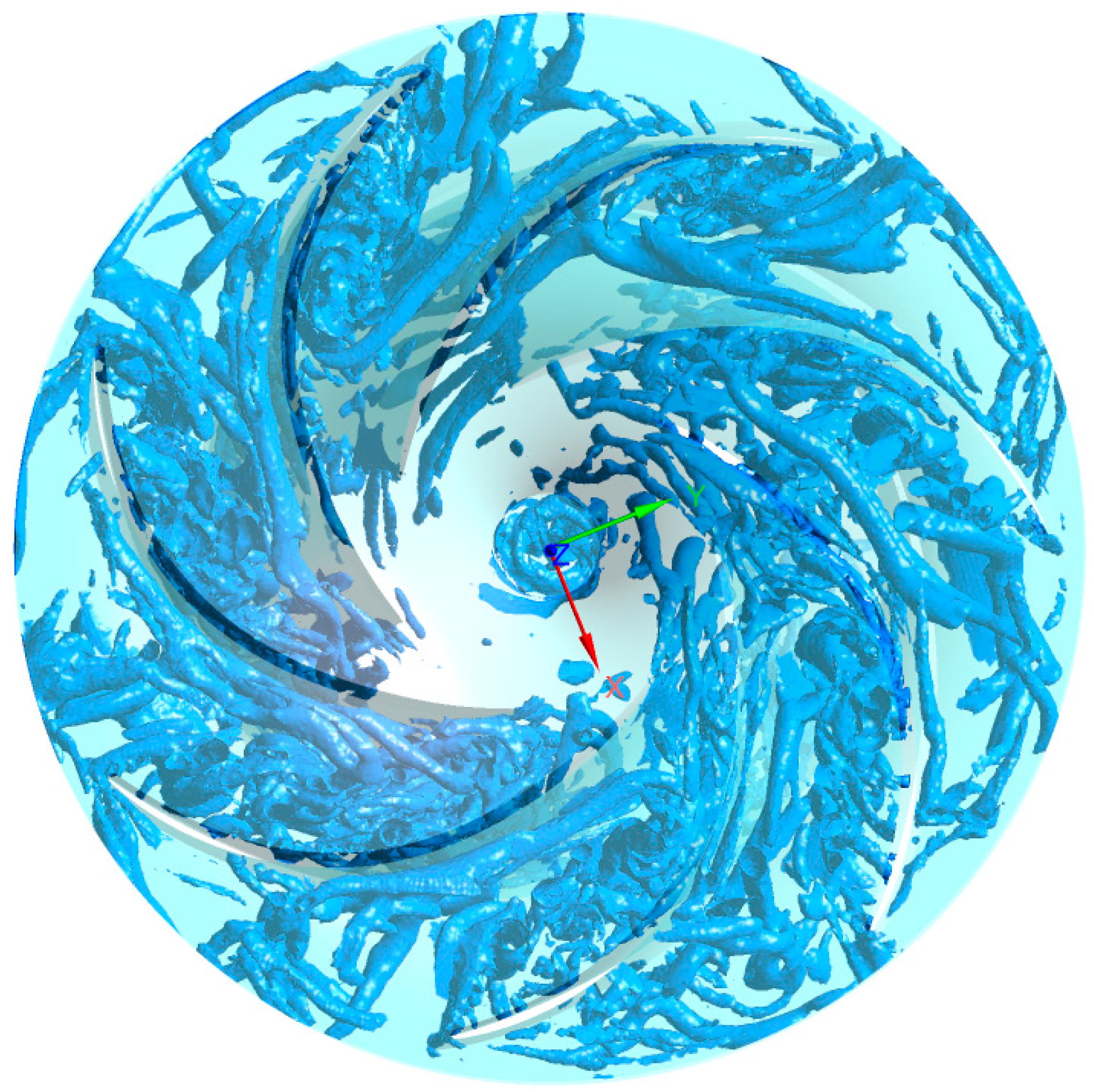
The pressure and velocity distribution of the fluid are more uniform before flowing in the runner at the rated load 100%Pn. However, it has a small impact on the head of the blades. As such, after the water flows in the runner, the velocity gradient changes rapidly, and the turbulence moves violently. Theoretically, the velocity direction of the inlet flow is basically the same as the tangential direction of the bone line of the blade of the runner. This would mean that there is no-impingement at the runner inlet for the best efficiency point case. As is shown in Figure 3, due to the rotor-stator interaction, there is a small angle of attack near the head of the blades, that is, the inflow is not satisfied with the no-impingement condition, and the high speed inflow is impacted by the blades at the runner inlet. The flow pattern changes and tries to be unstable. The water flows through a channel along the inner arc and the back arc of the blades after obstructions of the head of the blades. Under the influences of the viscous action of the curved blade surface and the inverse pressure gradient caused by the projecting objects, a flow separation is generated near the suction surface of the blades. The flow state is unstable, and the complex vortex structures are caused by the dehydration form in the blade path, that is, the channel vortex. As shown in Figure 4, the channel vortex consists of a series of the different scale vortex, occupying 1/3 of space of the blade path. The channel vortex goes downstream along the suction surface, converging, interfering with other vortexes, continuously cascading and bifurcating, and then evolves into many small-scale eddies (see Section 3.3).
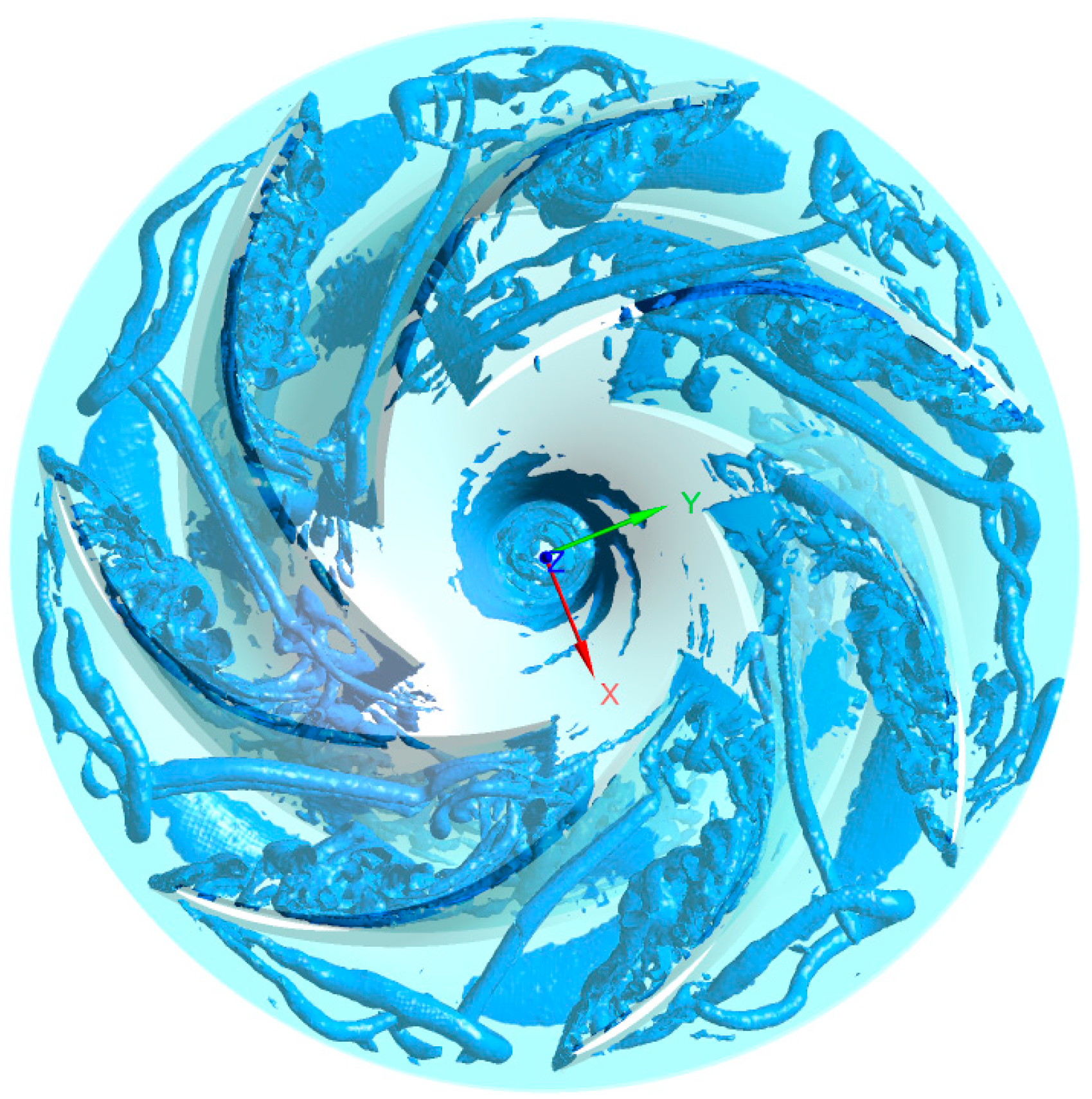
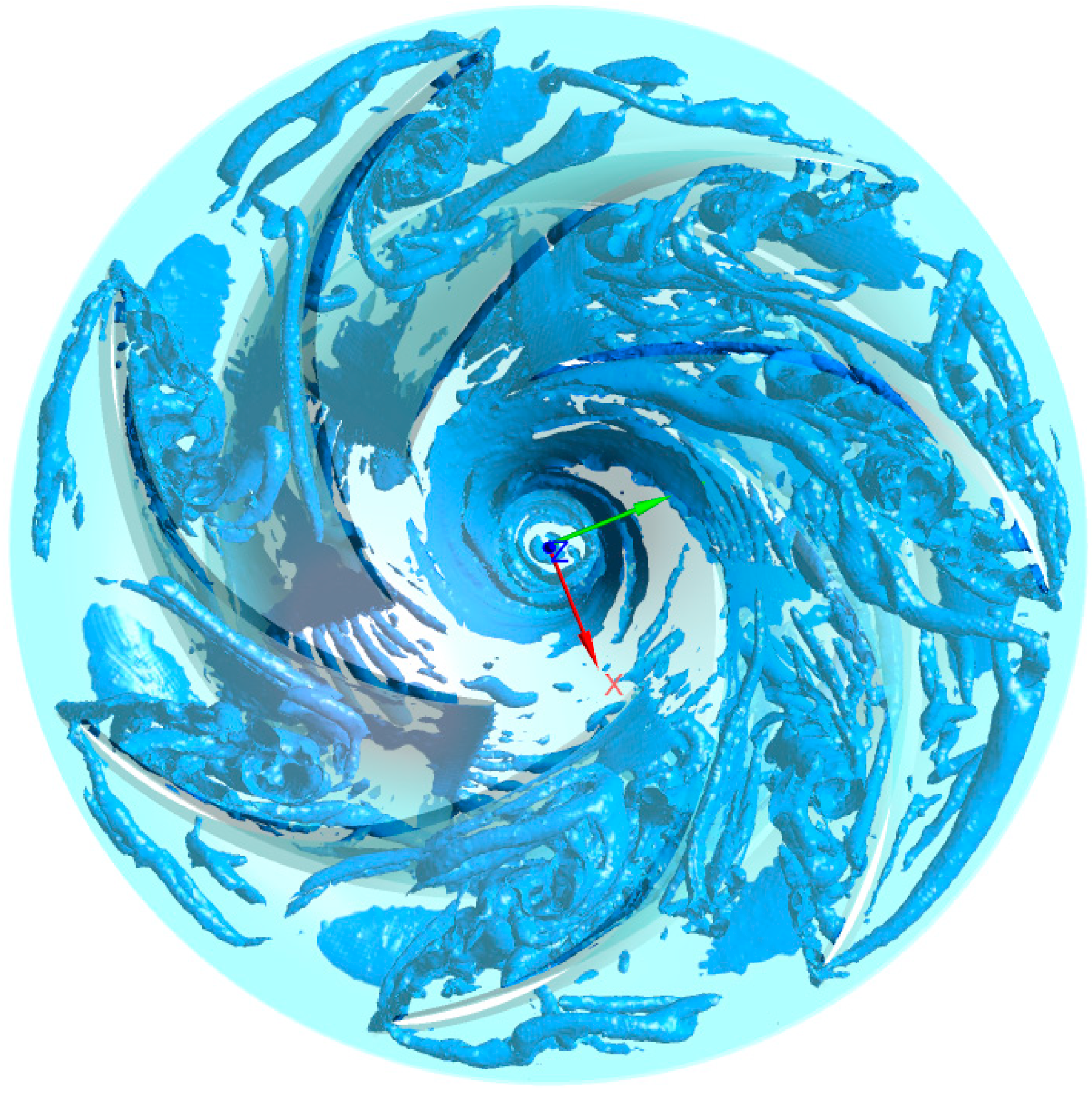
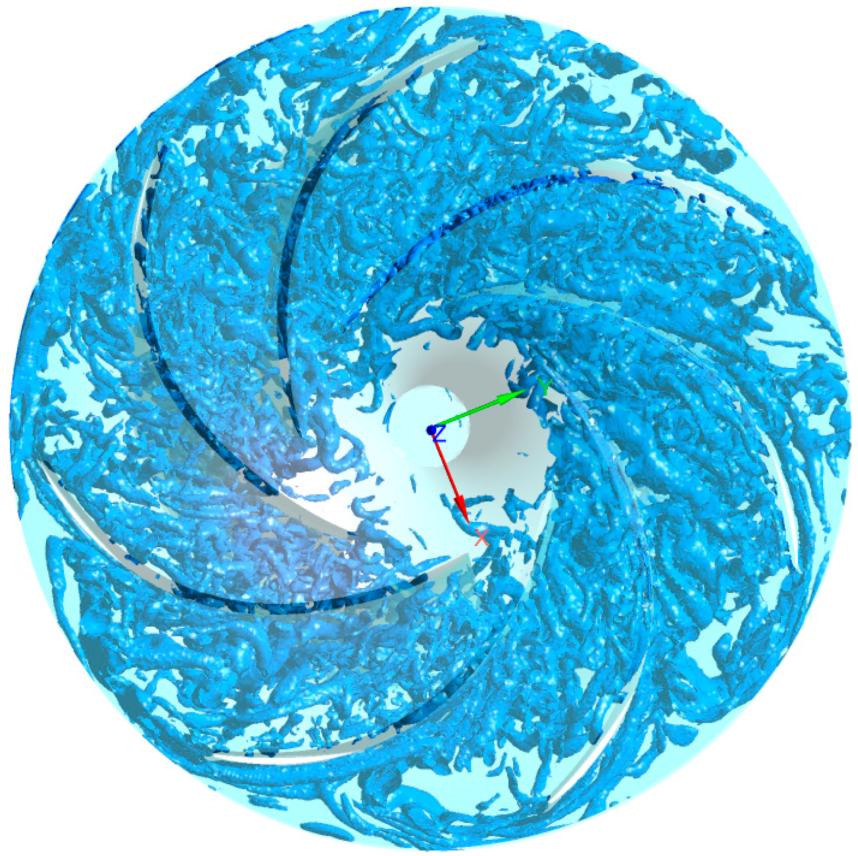
With the decrease of the guide opening degree, the flow decreases, while the angle of attack at the head of the blades increases. The impact on the head of the blades is strengthened. The flow separation in the channel becomes more and more significant. The scale of the channel vortex increases, and the distribution of the tubular vortex and horseshoe vortex are very obvious, indicating that the flow state is unstable, as shown in Figure 5, Figure 6 and Figure 7. With the further decrease of the guide opening degree, the flow disorder in the runner aggravates because the flow channel of the guide vane is limited. The scale of the channel vortex is relatively small but took up much more space, and the distribution of the flow patterns in each channel is unsymmetrical. It is shown in Figure 8 that a relatively large number of vortex structures occur in the region of the guide vanes at 1%Pn, and the scale of the vortex structures in the runner is small but more uniform, and almost occupies the whole runner space.
3.2. Different Forms of Channel Vortex
From Figure 4, Figure 5, Figure 6, Figure 7 and Figure 8, it can be seen that the vortex structures in the runner is different at the different angles of attack. When the angle of attack is small, the stable spiral point develops into a smaller vortex structure in the flow path, that is, the horn vortex, which makes the main vortex develop asymmetrically. When the angle of attack is large, it develops into a horseshoe vortex, restraining the main vortex asymmetric development by restraining the main vortex core. As the angle of attack increases, it becomes a complex multi-vortex system (called the main vortex system). As shown in Figure 7, the main vortex not only also contains the complex secondary vortex structures, but also contains a variety of unsteady motion modes for the unsteady horseshoe vortex. For a middle angle of attack, many types of vortex are developed in the runner, for example, the horn vortex, horseshoe vortex and the tubular vortex.
Restricted by the experimental measurement and analysis method, the study on vortex system is still limited. But research about vortexes has been increasing in recent years [26,27]. The structures and functions of all kinds of vortexes are different. For example, the horn vortex, also called the vertical vortex, spiral vortex, tornado vortex and so on, is the result of 3D flow separation. The surface morphology of the horn vortex is separation spiral, a tornado shape. The occurrence frequency of the horn vortex is higher. While the structure of the vortex is smaller and the vortex intensity is weak, it stills effect hydrodynamics and the development of the main vortex system through the main vortex.
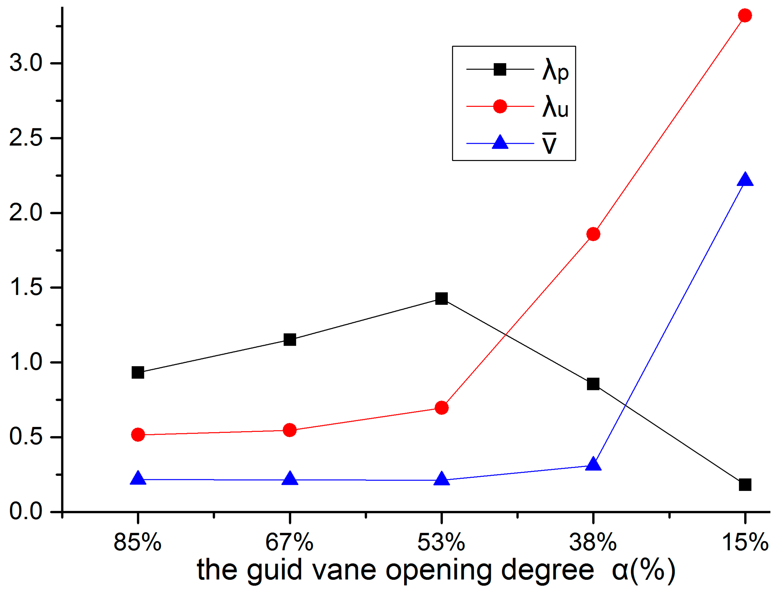
In order to quantitatively describe the shape of vortices for the different inlet angles of attack in the transitional process, pressure non-uniformity index , velocity non-uniformity index and eddy viscosity mean values are defined respectively.
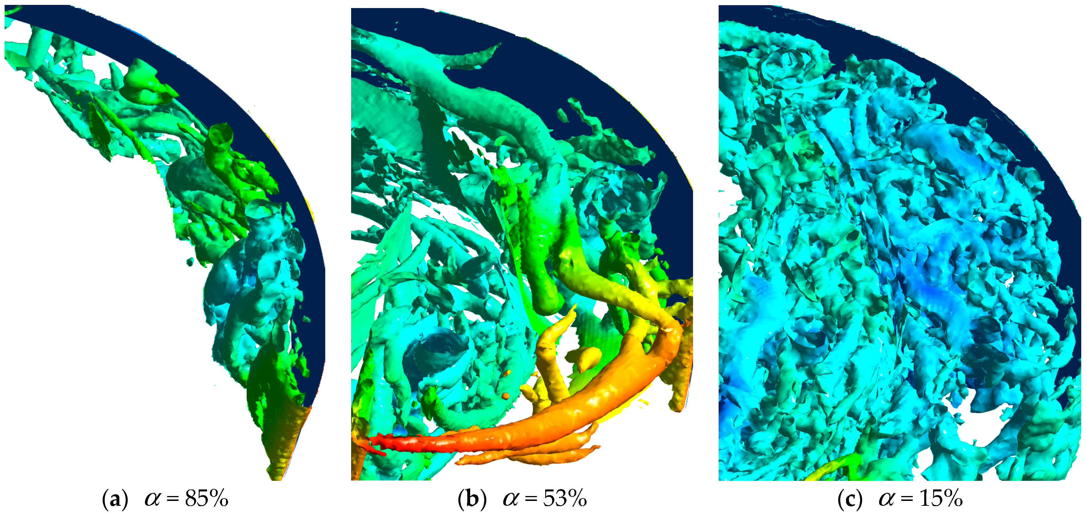
where, , are the maximum pressure and the minimum pressure in the surviving space of a certain scale vortex respectively. , are the maximum velocity and the minimum velocity in the blade passage respectively, and is the eddy viscosity at the midline of the blade passage, , respectively are the reference pressure and velocity, the average pressure and velocity at the inlet are taken in this paper. Figure 9 shows vortex structures in the different inlet angles of attack (10% characteristic scale) in the transitional process. Figure 10 shows the pressure non-uniformity index, the velocity non-uniformity index and the eddy viscosity mean values in the different inlet angles of attack in the transitional process. From the distribution trend, the inlet angle of attack in the rated power condition is small, the flow separation is relatively weak, the vortex mainly develops at the back of the blade, and the space occupied by vortex structures is small, it is a horn vortex. As the guide vane opening decreases, the inlet angle of attack increases. The degree of the flow separation becomes more and more obvious, the pressure and velocity non-uniformity index clearly increase, the vortex structure area is wider, the change of the eddy viscosity is relatively slow, and many vortex structures exist in the blade passage. Besides horn vortex, tubular vortex and horseshoe vortex also exist. This may be mainly caused by inhomogeneous pressure and high-pressure gradients. With the further reduction of the guide vane opening, the inlet angle of attack increases. Although the pressure non-uniformity index decreases obviously, the velocity non-uniformity index and the eddy viscosity increase rapidly and greatly. Tubular vortex gradually develops into horseshoe vortex. In addition, a turning point exists at 53%. Two sections are clearly seen, where corresponding powers are 1%Pn–50%Pn and 50%Pn–100%Pn. The positions of these two sections are very close to the hydraulic vibration area and stable operation area, where corresponding powers are generally 1%Pn–60%Pn and 60%Pn–100%Pn.
During study of the turbulence, we often pay much attention to the development of the main vortex system. Generally, the existence and characteristics of the horn vortices have been rarely observed. Tubular vortices are the result of the development of the flow structures in the blade channel. Because the tubular vortices belong to the twisted vortex structures, the tubular vortices have circumferential components, and the shape effect by the adjacent blade wall is like a pipe, which is quite difficult to capture through general numerical simulations. Therefore, the tubular vortices are rarely mentioned in the literature. In this simulation, the tubular vortices captured in the middle of the channel disappeared at the channel outlet. The vorticity of the horseshoe vortices is strong, and the formation mechanism of the vortex is relatively simple compared with the tubular vortex. Some scholars have done a lot of research on horseshoe vortex on a plane two-dimensional flow field. Chen et al. [28] studied the horseshoe vortex produced by the flow around the cylinder. It’s still difficult to study the horseshoe vortex in the three-dimensional twisted space.
3.3. Cascade Characteristics of Vortex Structures
According to the definition of the intersection ratio for a single eddy of scale A intersecting N eddies of scale B at a given instant in document [29], the survival volume ratio of the adjacent scale vortex N(A,B) is defined as:
where, is the survival volume of the eddy of scale A in space, is the survival volume of the eddy of the adjacent and small-scale B. The evolution of the large-scale eddies into the small-scale eddies in turbulence flow is analyzed.
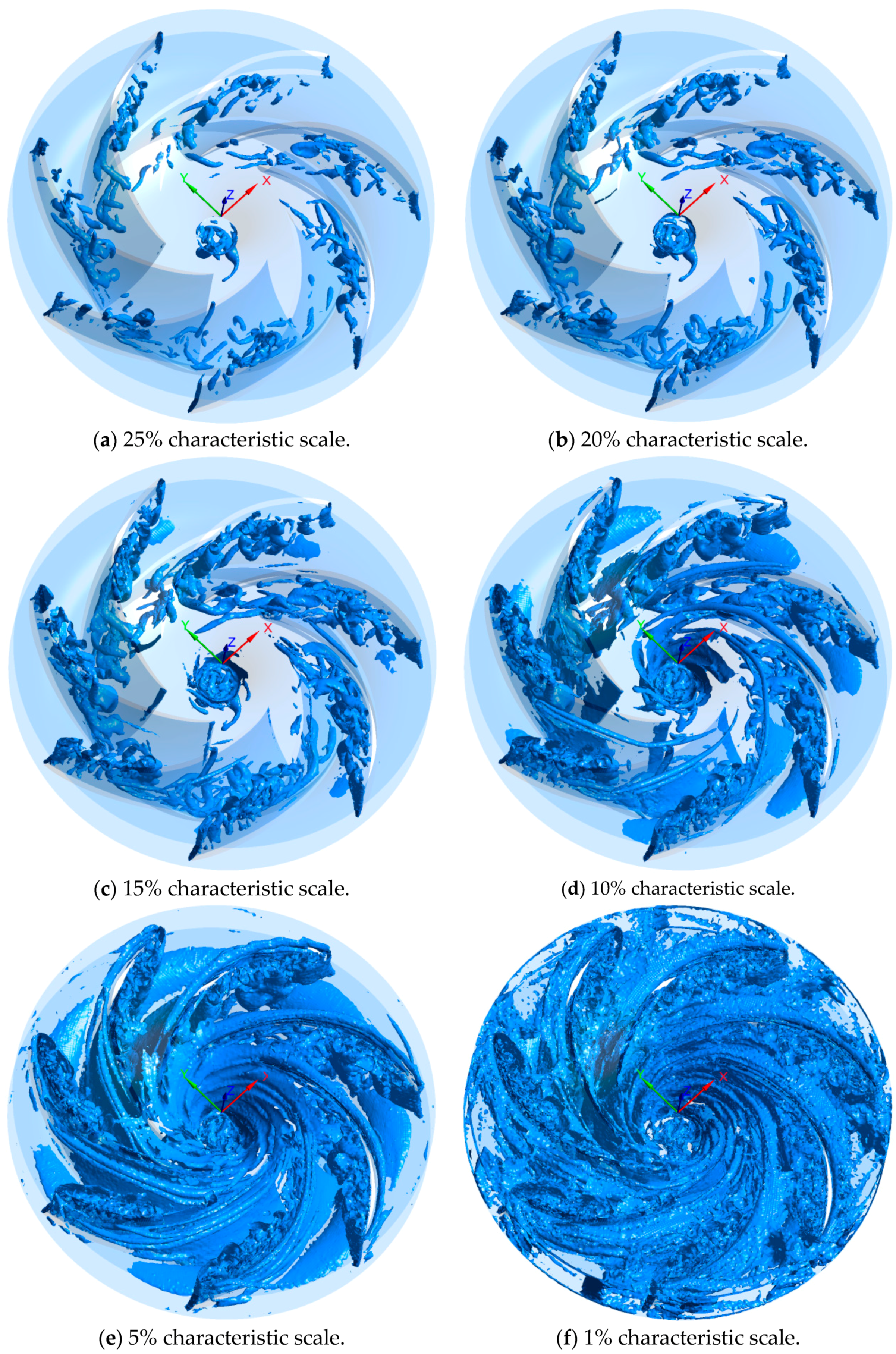
According to the decomposition principle, the square root of the inlet area of the blade channel is defined as the characteristic scale of the channel in this paper. Taking the characteristic scale as the datum, the survival volume of the 6 grade decomposition eddies for 100%Pn relative to the characteristic scale, 25–1% is given, as shown in Figure 11.
The survival volume of the “large scale” 25% vortex is herein relatively small, while the survival rate of the “small scale” 1% vortex is very large, and almost occupied the whole channel. It clearly shows the spatial distribution of the different scale vortex structures. The smaller the eddy scale is, the greater vortex volume is. This is mainly due to the instability of the vortex structures, which interfere with each other and bifurcate, and evolve into new complex vortex structures. Large-scale eddies break into the small-scale eddies, and then the small eddies break into smaller eddies, and in each evolution the scales of the eddies become smaller, the number of eddies increases, and more space is occupied.
The survival volume ratios of the adjacent scale vortex N(A,B) for 100%Pn is shown in Table 3. It can be seen that the survival volume of the adjacent vortices increases by 1.2 to 1.6, and the survival volume rate of the “middle-scale” vortex of 15% to 10% is the largest, up to 1.549, and the survival volume ratio of the adjacent scale vortex far away from the scale is gradually reduced.
The above analyses of the survival volume reveal the process of turbulent kinetic energy dissipation in the channel, that is, the existence of a large number of small scale eddies formed in the middle and rear segments of the cascade (as shown in Figure 9f) increases the eddy turbulence viscosity in the flow field, resulting in the flow damping being added, so energy dissipation increases largely, which explains why the turbulent kinetic energy in the vicinity of the outlet will greatly increase.
The middle line of the middle surface in the blade channel is evenly divided into 5 equal parts, and equal points P1–P4 are recorded along the direction of the flow. The turbulent kinetic energy and the eddy viscosity at P1–P4, as shown in Table 4, increase gradually along the channel. Especially in the rear part of the blade channel, the turbulent kinetic energy and the eddy viscosity become very large. It indicates that the small-scale vortex along the flow direction increases sharply, and as the turbulent energy dissipation aggravated, a clear dissipative passage was formed.
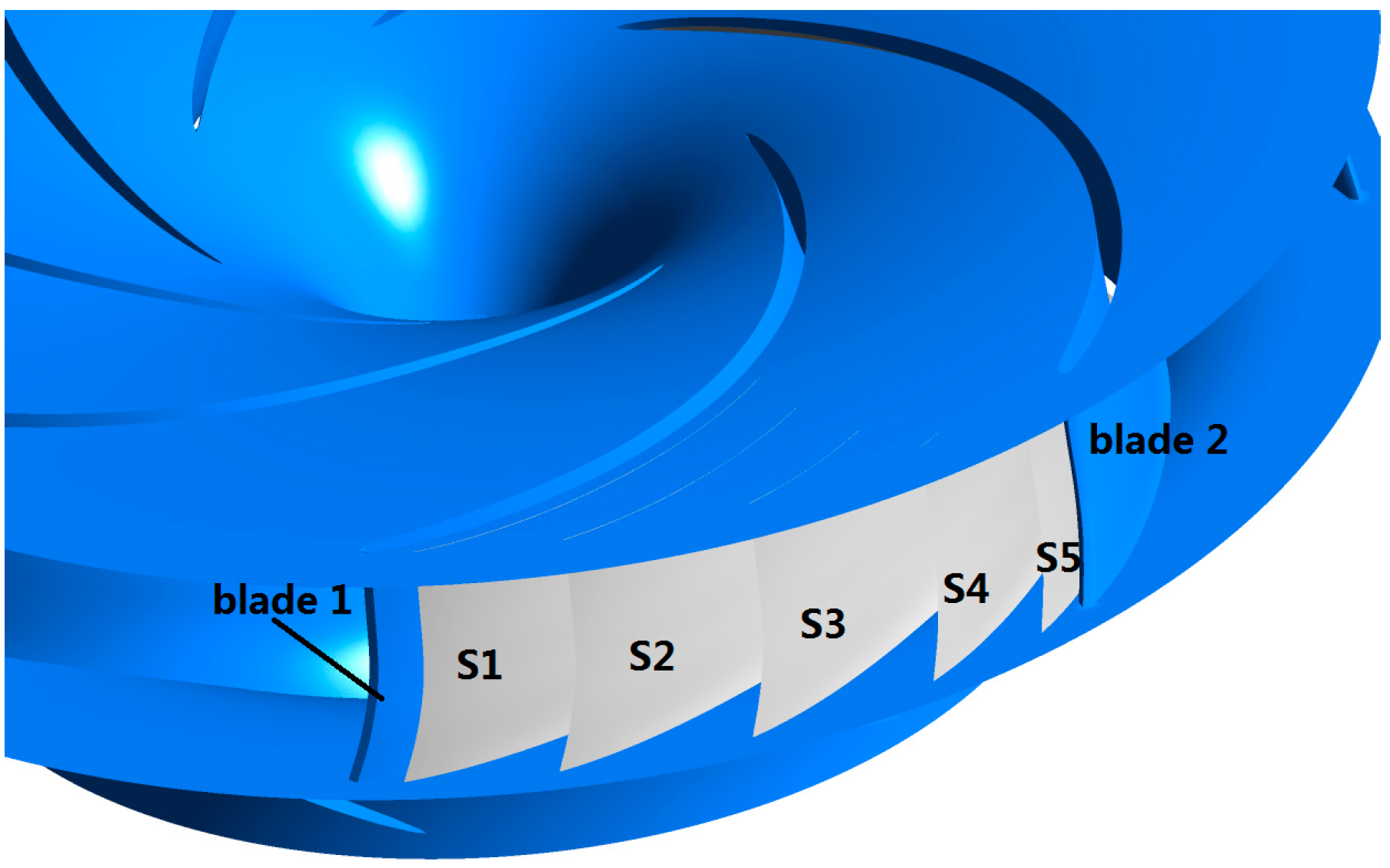
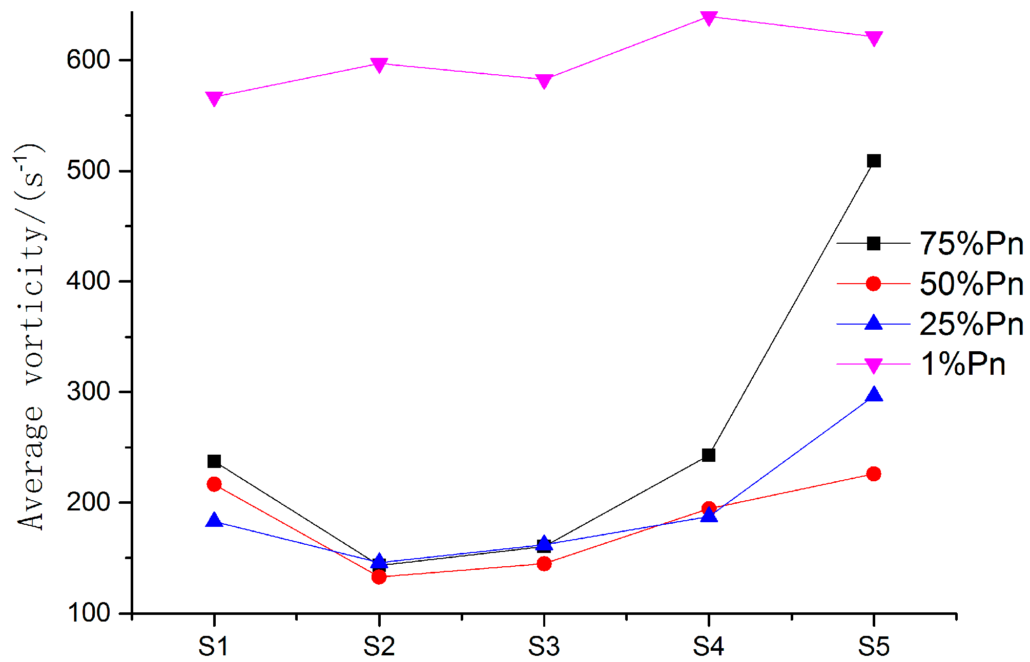
In order to reveal vortex evolution rule by observing the distribution of the vortex, we divide one channel into 4 equal parts along the spanwise direction. The divided monitored surfaces are defined as S1 to S5, that is, S1 near the pressure surface, S2 at the 1/4 of the channel, S3 in the middle surface of the channel, S4 at the 3/4 of the channel, and S5 near the suction surface, as shown in Figure 12. For the sake of convenient observation, the vortex structures are usually decomposed into two components: streamwise vortices and spanwise vortices. However, the flow direction in the runner is very complicated, and it is difficult to decompose a vortex into streamwise vortices and spanwise vortices. Therefore, the average vorticity value is used in this paper. The average vorticity of the monitored surfaces in the non-full rated operating states is shown in Figure 13. It can be seen that, in addition to 1%Pn, the vortex lines of the monitored surfaces are shaped like a tubular fishhook, the average vorticity at S5 near suction surface is the largest, the average vorticity at S1 near pressure surface takes second place, and the others are S4, S3 and S2 in turn. Vortex structure scale in the runner at 1%Pn is small, and almost occupies the whole runner space. Therefore, the change of the average vorticity at the monitored surfaces at 1%Pn is not obvious. According to Figure 5, Figure 6, Figure 7 and Figure 8, it is known that the vortex structure is larger as fluid degenerated near the suction surface at other non-full rated operating states. There is a small deviation between the cutting direction of the blade bone line and the inlet flow. Therefore, the average vorticity near the surface is larger. The number of the eddies in the region with a greater average vorticity is large, and the vortex structure near the suction surface is the largest one, which indicates that the flow separation near the suction surface is relatively significant. The evolution of the vortex structures is accompanied with the dissipation of the energy, and the dissipation coefficient of the vortex energy can be defined as: , where stands for the vortex energy, stands for the fluid flow, and stands for the water head. It can be obtained: under the same water head, the dissipation coefficient of the vortex energy 1%Pn is the largest, and the others are 25%Pn, 50%Pn and 75%Pn in sequence. It is also known that the smaller the guide vane opening degree, the larger dissipation coefficient of the vortex energy, and also the larger the energy loss of the vortex structure.
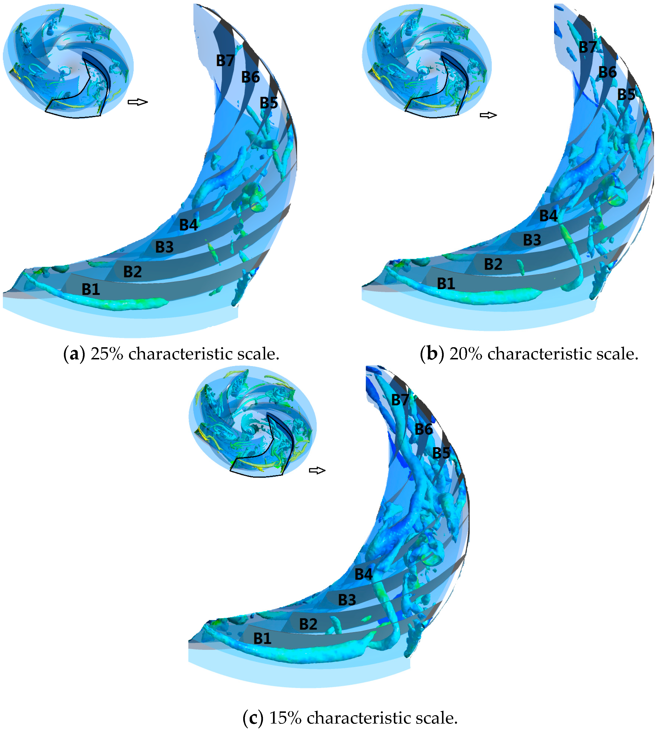
Similarly, in order to better reveal a vortex evolution rule, we divide the region of two blades into eight equal parts along the flow direction, defining the divided surfaces as site reference planes B1 to B7, as shown in Figure 14. The three-dimensional space of the blade passage is extremely complex, so the shapes and sizes of B1–B7 are differently shown in figures. Only the location of the vortices has been analyzed here. As shown in Figure 14, most of 25% vortices are grouped in between B3 and B5 (i.e., 38% to 63% region of the blade passage along flow direction), most of 20% vortices are grouped in between B3 and B6 (i.e., 38% to 75% region of the blade passage along flow direction), most of 15% vortices are grouped in between B3 and B7 (i.e., 38% to 100% region of the blade passage along flow direction). This indicates that large scale vortices evolve into large scale vortices and small-scale vortices become more and more common in the blade passage along the flow direction, especially in the rear segment of the bale passage.
For the effect of time, according to our research, the distribution of the different scales vortices with rated condition 100%Pn at two different instants is very similar. This indicates that the geometric characteristics of the flow passage match well with the flow fields at the rated condition 100%Pn. The evolution of the vortex has a certain characteristic of “definite”. It is consistent with the condition that the unit runs smoothly with rated condition.
3.4. Similarity Analysis of Vortex Cascade and Dissipation Features
Similarity of the solutions was found for the evolution of poly disperse droplets in vortex flows [30]. Cavitating similarity solutions existed for a vortex of which both core diameter and circulation grow with the square root of the axial coordinate [31]. In order to explore the similarity of the vortex cascade and dissipation features of the turbulent flow for a hydro-turbine, numerical simulation of three-dimensional turbulent flow for the model and the prototype pump-turbine with rated case was conducted with LES. For convenience and completeness, we give the main conclusions in this paper:
Vortex structures of the prototype and a model with 1:10 scale were quantitatively and qualitatively compared and were found to be very similar in the spatial distributions, however the vortex structures of the model are relatively rough and concentrated. Also, the survival volume ratio of the adjacent scale vortex is basically the same. The vorticity, the eddy viscosity, and the turbulent kinetic energy of the prototype and the model satisfy the similarity. As such, the vortex cascade and the dissipation features of the turbulent flow should be similar.
4. Conclusions
In this paper, a large eddy simulation method based on the dynamic subgrid stress model was used to calculate the 3D unsteady turbulent flow in a pump turbine in transitional process from rated load to no-load states. The unsteady flow structure was analyzed, and the survival volume of the different scale eddies was well obtained. The energy dissipation channel was found. Developing hydrodynamic instabilities corresponds to an eddy cascade developing in the energy. According to the analyses, the following conclusions are drawn.
- (1)
- Due to the inconsistency between streamwise direction of the inlet flow and tangential direction of the bone line of the blade, angle of attack exists. Fluid flows through inner arc and back arc of the blade after the obstruction of the head of the blades. Under the influences of the viscous action of the curved blade surface and the inverse pressure gradient caused by the projecting objects, the flow separation is generated near the suction surface of the blade, and the flow state is unstable. The complex vortex structures caused by the dehydration are formed in the blade path, that is, the channel vortex. The vortex structure in the runner is different for the different angles of attack. When the angle of attack is small, the rupture of the tubular vortices will lead to developments of the spiral vortices into the horn vortex in the blade channel. When the angle of attack is large, it develops into a horseshoe vortex. When the angle of attack is medium, both horn vortex and horseshoe vortex are formed in the blade passage. The larger the angle of attack, the more complex the vortex system.
- (2)
- The “large scale” eddies at the blade passage have low survival rates, while “small scale” eddies have a high one. The volume ratio of the adjacent scale vortex is about 1.2–1.6.
- (3)
- The average vorticity near wall surfaces is large, and that of suction surface is higher than that of pressure surface. The flow separation near the surface is relatively significant. The average vorticity in the middle of the runner is secondary. The smaller the guide vane opening degree, the larger the energy loss of the vortex structure.
- (4)
- Turbulent kinetic energy near the outlet increases significantly. The existence of a large number of small-scale eddies which are formed in the middle of the channel increases turbulent viscosity in the flow field, causing the increase of the energy dissipation.
- (5)
- Large scale vortices evolve into large scale vortices, and small-scale vortices become more and more common in the blade passage along flow direction, especially in the rear segment of the bale passage.
- (6)
- Vorticity, eddy viscous, turbulent kinetic energy have similarities in their numerical values. The vortex cascade and dissipation features of the turbulent flow are also similar.
Author Contributions
L.Z. has contributed most to the conception, guidance, and revising of the manuscript. The data acquisition and analysis were done by X.H. The manuscript was written by X.H.
Funding
This work was supported by the National Natural Science Foundation of China (Grant No. 51279071) and the Foundation of the Ministry of Education of China for Ph.D candidates in University (Grant No. 2013531413002).
Acknowledgments
All authors are very grateful to the editor and the three anonymous reviewers for their valuable comments, which have greatly improved the paper.
Conflicts of Interest
The authors declare no conflict of interest.
Nomenclature
| —rotation speed of the runner (rpm) |
| —time (s) |
| —co-ordinate component of Cartesian system (m) |
| —component of flow velocity (m/s) |
| (m/s2) |
| —filtered component of flow velocity (-) |
| —test filtered component of flow velocity (-) |
| —kinetic viscosity of fluid (Pa·s) |
| —eddy viscosity of fluid (Pa·s) |
| —filtered pressure divided by mass density (-) |
| —pressure non-uniformity index (-) |
| —velocity non-uniformity index (-) |
| —eddy viscosity mean values (Pa·s) |
| —the maximum pressure in the surviving space of a certain scale vortex (Pa) |
| —the minimum pressure in the surviving space of a certain scale vortex (Pa) |
| —the maximum velocity in blade passage (m/s) |
| —the minimum velocity in blade passage (m/s) |
| —the eddy viscosity at the midline of blade passage (Pa·s) |
| —the reference pressure (Pa) |
| —the reference velocity (m/s) |
| —liquid mass density (kg/m3) |
| —Kronecker’s delta (-) |
| —strain rate tensor (-) |
| —grid width in i direction (m) |
| —SGS stress (-) |
| —Leonard stress (-) |
| —Cross stress (-) |
| —Reynolds stresses (-) |
| Pn—rated power (W) |
| T—rotation period (s) |
| —attack angle (°) |
| —survival volume ratio of adjacent scale vortex (-) |
| —survival volume of the eddy of scale A in space (m3) |
| —survival volume of the eddy of scale B in space (m3) |
| —dissipation coefficient of vortex energy (J·s·m4) |
| —vortex energy (J) |
| —fluid flow (m3/s) |
| —water head (m) |
| —the guide vane opening degree (%) |
References
- Richardson, L.F. Weather Prediction by Numerical Process; Cambridge University Press: Cambridge, UK, 1922. [Google Scholar]
- Kolmogorov, A.N. The local structure of turbulence in incompressible viscous fluid for very large Reynolds number. Proc. Math. Phys. Sci. 1991, 434, 9–13. [Google Scholar] [CrossRef]
- Davidson, P.A. A Voyage through Turbulence; Cambridge University Press: Cambridge, UK, 2011. [Google Scholar]
- Deusebio, E.; Boffetta, G.; Lindborg, E.; Musacchio, S. Dimensional transition in rotating turbulence. Phys. Rev. E Stat. Nonlinear Soft Matter Phys. 2014, 90, 023005. [Google Scholar] [CrossRef] [PubMed]
- Marino, R.; Mininni, P.D.; Rosenberg, D.; Pouquet, A. Inverse cascades in rotating stratified turbulence: Fast growth of large scales. EPL 2013, 102, 44006. [Google Scholar] [CrossRef]
- Aluie, H.; Kurien, S. Joint downscale fluxes of energy and potential enstrophy in rotating stratified Boussinesq flows. EPL 2011, 96, 44006. [Google Scholar] [CrossRef] [Green Version]
- Nastrom, G.D.; Gage, K.S.; Jasperson, W.H. Kinetic energy spectrum of large-and mesoscale atmospheric processes. Nature 1984, 310, 36–38. [Google Scholar] [CrossRef]
- Gage, K.S.; Nastrom, G.D. Theoretical interpretation of atmospheric wavenumber spectra of wind and temperature observed by commercial aircraft during gasp. J. Atmos. Sci. 1986, 43, 729–740. [Google Scholar] [CrossRef]
- Byrne, D.; Zhang, J.A. Height-dependent transition from 3-D to 2-D turbulence in the hurricane boundary layer. Geophys. Res. Lett. 2013, 40, 1439–1442. [Google Scholar] [CrossRef] [Green Version]
- Young, R.M.B.; Read, P.L. Forward and inverse kinetic energy cascades in Jupiter’s turbulent weather layer. Nat. Phys. 2017, 13, 1135–1140. [Google Scholar] [CrossRef]
- Miloshevich, G.; Morrison, P.J.; Tassi, E. Direction of cascades in a magnetofluid model with electron skin depth and ion sound Larmor radius scales. Phys. Plasmas 2018, 25, 072303. [Google Scholar] [CrossRef]
- Alexakis, A.; Biferale, L. Cascades and transitions in turbulent flows. Phys. Rep. 2018, 767–769, 1–101. [Google Scholar] [CrossRef]
- Fortova, S.V. Eddy cascade of instabilities and transition to turbulence. Comput. Math. Math. Phys. 2014, 54, 553–560. [Google Scholar] [CrossRef]
- Zhang, H.; Chen, D.; Guo, P.; Luo, X.; George, A. A novel surface-cluster approach towards transient modeling of hydro-turbine governing systems in the start-up process. Energy Convers. Manag. 2018, 165, 861–868. [Google Scholar] [CrossRef]
- Widmer, C.; Staubli, T.; Ledergerber, N. Unstable characteristics and rotating stall in turbine brake operation of pump-turbines. J. Fluids Eng. 2011, 133, 041101. [Google Scholar] [CrossRef]
- Trivedi, C.; Cervantes, M.J.; Gandhi, B.K.; Dahlhaug, O.G. Transient pressure measurements on a high head model francis turbine during emergency shutdown, total load rejection, and runaway. J. Fluids Eng. 2014, 136, 121107. [Google Scholar] [CrossRef]
- Hu, J.; Yang, J.; Zeng, W.; Yang, J. Transient pressure analysis of a prototype pump turbine: Field tests and simulation. J. Fluids Eng. 2018, 140, 071102. [Google Scholar] [CrossRef]
- Yang, J.; Hu, J.; Zeng, W.; Yang, J. Transient pressure pulsations of prototype Francis pump-turbines. J. Hydraul. Eng. 2016, 47, 858–864. [Google Scholar]
- Xia, L.; Cheng, Y.; Cai, F. Pressure pulsation characteristics of a model pump-turbine operating in the S-shaped Region: CFD simulations. Int. J. Fluid Mach. Syst. 2017, 10, 287–295. [Google Scholar] [CrossRef]
- Zhang, L.; Wang, W.; Guo, Y. Numerical simulation of flow features and energy exchange physics in near-wall region with fluid-structure interaction. Int. J. Mod. Phys. B 2008, 22, 651–669. [Google Scholar] [CrossRef]
- Hu, X.; Zhang, L. Numerical simulation of unsteady flow for a pump-turbine in transition cases with large-eddy simulation. J. Hydraul. Eng. 2018, 49, 492–500. [Google Scholar]
- Germano, M.; Piomelli, U.; Moin, P.; Cabot, W.H. A dynamic subgrid scale eddy viscosity model. Phys. Fluids A Fluid Dyn. 1991, 3, 1760–1765. [Google Scholar] [CrossRef]
- Zhang, L.; Guo, Y.; Wang, W. Large eddy simulation of turbulent flow in a true 3D Francis hydro turbine passage with dynamical fluid-structure interaction. Int. J. Numer. Methods Fluids 2007, 54, 517–541. [Google Scholar] [CrossRef]
- Gabl, R.; Innerhofer, D.; Achleitner, S.; Righetti, M.; Aufleger, M. Evaluation criteria for velocity distributions in front of bulb hydro turbines. Renew. Energy 2018, 121, 745–756. [Google Scholar] [CrossRef]
- Guo, T.; Zhang, L. Numerical study on turbulence characteristics in Francis turbine under small opening condition. Eng. Mech. 2015, 32, 222–230. [Google Scholar]
- Kudela, H.; Malecha, Z.M. Investigation of unsteady vorticity layer eruption induced by vortex patch using vortex particles method. J. Theor. Appl. Mech. 2007, 45, 785–800. [Google Scholar]
- Kudela, H.; Malecha, Z.M. Eruption of a boundary layer induced by a 2D vortex patch. Fluid Dyn. Res. 2009, 41, 055502. [Google Scholar] [CrossRef]
- Chen, Q.; Qi, M.; Li, J. Kinematic characteristics of horseshoe vortex upstream of circular cylinders in open channel flow. J. Hydraul. Eng. 2016, 47, 158–164. [Google Scholar]
- Cardesa, J.I.; Vela-Martín, A.; Jiménez, J. The turbulent cascade in five dimensions. Science 2017, 357, 782–784. [Google Scholar] [CrossRef] [Green Version]
- Dagan, Y.; Greenberg, J.B.; Katoshevski, D. Similarity solutions for the evolution of polydisperse droplets in vortex flows. Int. J. Multiph. Flow 2017, 97, 1–9. [Google Scholar] [CrossRef]
- Bosschers, J.; Janssen, A.A.; Hoeijmakers, H.W.M. Similarity solutions for viscous cavitating vortex cores. J. Hydrodyn. Ser. B. 2008, 20, 679–688. [Google Scholar] [CrossRef]
Figure 1.
Configuration of computational domains (in meter): (a) Vertical and overhead views; (b) Overall view.
Figure 1.
Configuration of computational domains (in meter): (a) Vertical and overhead views; (b) Overall view.

Figure 2.
Grids in centerplane of guide vanes.

Figure 3.
Velocity diagram of the Z = 0 at 100%Pn.

Figure 4.
Vortex structures at 100%Pn (10% characteristic scale).

Figure 5.
Vortex structures at 75%Pn (10% characteristic scale).

Figure 6.
Vortex structures at 50%Pn (10% characteristic scale).

Figure 7.
Vortex structures at 25%Pn (10% characteristic scale).

Figure 8.
Vortex structures at 1%Pn (10% characteristic scale).

Figure 9.
Vortex structures in different inlet attack angles (10% characteristic scale).

Figure 10.
Non-uniformity indexes in different inlet attack angles.

Figure 11.
The survival volume of different scale eddies at 100%Pn.

Figure 12.
Monitored surfaces.

Figure 13.
Average vorticity at monitored surfaces in non-full rated operating states.

Figure 14.
Vortex structures in one blade passage at 50%Pn.


Table 1.
Radius of the sections.
| Section | Radius (m) | Section | Radius (m) | Section | Radius (m) | Section | Radius (m) |
|---|---|---|---|---|---|---|---|
| S1 | 1.5009 | S10 | 1.0540 | S19 | 0.4173 | d7 | 2.1403 |
| S2 | 1.4553 | S11 | 0.9967 | S20 | 0.4088 | d8 | 2.1202 |
| S3 | 1.4096 | S12 | 0.9359 | S21 | 0.4066 | d9 | 2.0921 |
| S4 | 1.3644 | S13 | 0.8734 | d1 | 1.9670 | d10 | 2.0470 |
| S5 | 1.3176 | S14 | 0.8093 | d2 | 2.0064 | d11 | 2.0024 |
| S6 | 1.2677 | S15 | 0.7391 | d3 | 2.0719 | d12 | 1.9654 |
| S7 | 1.2161 | S16 | 0.6629 | d4 | 2.1124 | d13 | 1.9475 |
| S8 | 1.1637 | S17 | 0.5825 | d5 | 2.1404 | d14 | 1.9475 |
| S9 | 1.1103 | S18 | 0.4880 | d6 | 2.1469 | d15 | 3.1097 |
Table 2.
Computation parameters.
| Condition | 100%Pn | 75%Pn | 50%Pn | 25%Pn | 1%Pn |
|---|---|---|---|---|---|
| The guide vane opening degree (%) | 85% | 67% | 53% | 38% | 15% |
| Inlet velocity for the prototype (m/s) | 19.28 | 15.20 | 12.02 | 8.62 | 3.40 |
Table 3.
Survival volume ratio of adjacent scale vortex in runner at 50%Pn.
| Adjacent Scale | 0.25–0.2 | 0.2–0.15 | 0.15–0.1 | 0.1–0.05 | 0.05–0.01 |
|---|---|---|---|---|---|
| The survival volume ratio of adjacent vortex | 1.359 | 1.402 | 1.549 | 1.404 | 1.232 |
Table 4.
Eddy viscosity and turbulent kinetic energy.
| Equal Points | P1 | P2 | P3 | P4 |
|---|---|---|---|---|
| Eddy viscosity for 100%Pn (Pa·s) | 0.1187 | 0.1434 | 0.2613 | 0.3413 |
| Eddy viscosity for 75%Pn (Pa·s) | 0.1242 | 0.1513 | 0.2485 | 0.3373 |
| Eddy viscosity for 50%Pn (Pa·s) | 0.1522 | 0.1619 | 0.2483 | 0.2840 |
| Eddy viscosity for 25%Pn (Pa·s) | 0.1742 | 0.2384 | 0.2941 | 0.5403 |
| Eddy viscosity for 1%Pn (Pa·s) | 1.4615 | 1.8220 | 2.7041 | 2.8693 |
| Turbulent kinetic energy for 100%Pn (m2·s−2) | 8.59 | 21.03 | 39.312 | 45.467 |
| Turbulent kinetic energy for 75%Pn (m2·s−2) | 9.68 | 22.63 | 24.09 | 25.92 |
| Turbulent kinetic energy for 50%Pn (m2·s−2) | 6.19 | 14.27 | 16.03 | 16.86 |
| Turbulent kinetic energy for 25%Pn (m2·s−2) | 3.46 | 9.45 | 19.66 | 20.97 |
| Turbulent kinetic energy for 1%Pn (m2·s−2) | 22.34 | 19.22 | 58.56 | 51.66 |
© 2018 by the authors. Licensee MDPI, Basel, Switzerland. This article is an open access article distributed under the terms and conditions of the Creative Commons Attribution (CC BY) license (http://creativecommons.org/licenses/by/4.0/).
Share and Cite
MDPI and ACS Style
Hu, X.; Zhang, L. Vortex Cascade Features of Turbulent Flow in Hydro-Turbine Blade Passage with Complex Geometry. Water 2018, 10, 1859. https://doi.org/10.3390/w10121859
AMA Style
Hu X, Zhang L. Vortex Cascade Features of Turbulent Flow in Hydro-Turbine Blade Passage with Complex Geometry. Water. 2018; 10(12):1859. https://doi.org/10.3390/w10121859
Chicago/Turabian StyleHu, Xiucheng, and Lixiang Zhang. 2018. "Vortex Cascade Features of Turbulent Flow in Hydro-Turbine Blade Passage with Complex Geometry" Water 10, no. 12: 1859. https://doi.org/10.3390/w10121859
Note that from the first issue of 2016, this journal uses article numbers instead of page numbers. See further details here.