Article

A Method for Determining the Discharge of Closed-End Furrow Irrigation Based on the Representative Value of Manning’s Roughness and Field Mean Infiltration Parameters Estimated Using the PTF at Regional Scale

1
State Key Laboratory of Eco-hydraulics in Northwest Arid Region, Xi’an University of Technology, Xi’an 710048, China
2
Key Laboratory of Agricultural Soil and Water Engineering in Arid and Semiarid Areas, Ministry of Education, Northwest A&F University, Yangling 712100, China
*
Author to whom correspondence should be addressed.
Water 2018, 10(12), 1825; https://doi.org/10.3390/w10121825
Submission received: 25 October 2018 / Revised: 1 December 2018 / Accepted: 5 December 2018 / Published: 11 December 2018
(This article belongs to the Section Water Resources Management, Policy and Governance)

Abstract

:
Infiltration parameters and Manning’s roughness are essential input parameters for surface irrigation simulation models. Multiple points of infiltration experiments require time-consuming, costly data collection and problematic calculations of field mean infiltration parameters. This study estimated the field mean infiltration parameters and Manning’s roughness values on a regional scale, on the basis of closed-end furrow irrigation experiments conducted at 45 experimental sites on the Guanzhong plain, and evaluated the influence of Manning’s roughness on advance trajectory and performance indicators of closed-end furrow irrigation. Then, we present a functional normalization of the Kostiakov equation and pedotransfer function (PTF) to estimate the normalization factors. The proposed method can be used to estimate the field mean infiltration parameters using PTF and the represented Manning’s roughness to determine the optimal discharge of closed-end furrow irrigation. The results revealed that the advance trajectory and performance of closed-end furrow irrigation was not sensitive to variations of Manning’s roughness, which can be adopted as a representative value (i.e., 0.075) of the maize field. The normalization method was proven to be feasible for the Kostiakov equation, and the PTF reliably estimated the normalization factors. Last, the optimized values of the inflow discharge were determined using the proposed method, with various combinations of furrow lengths and bottom slopes in the study area, and also compared with the inflow discharge determined based on infiltration parameters and Manning’s roughness, which were inversed by SIPAR_ID. The results indicated that the inflow discharge values obtained through using the two methods were approximately equal, proving that the proposed method was reliable and easy to use in practice.

1. Introduction

Furrow irrigation is a widely used irrigation method, and closed-end furrow irrigation is one of its main variants. However, furrow irrigation systems are often inefficient because of poor irrigation performance [1,2]. Advanced simulation models of surface irrigation have been proven to be effective for evaluating system design and management, and for improving irrigation performance. Manning’s roughness and field mean infiltration parameters are essential input parameters for surface irrigation simulation models [3,4,5,6]. Therefore, it is vital to obtain realistic estimates of Manning’s roughness and field mean infiltration parameters.
In the actual surface irrigation process, numerous factors affect Manning’s roughness, and Manning’s roughness cannot be actually measured; the determination of Manning’s roughness is difficult, and wide ranges of variation have been reported [7,8]. Chow [9] reported Manning’s roughness values ranging from 0.02 to 0.40 for cultivated soils with no crop. Li and Zhang [10] determined that Manning’s roughness values can range from 0.02 to 0.05 with border irrigation. Zhang et al. [11], Bautista et al. [12], and Anwar et al. [13] have reported Manning’s roughness values of 0.02–0.40, 0.04–0.10, and 0.04–0.16, respectively. Other published studies have often used a representative value of Manning’s roughness to simulate furrow irrigation [14,15,16,17,18,19]. The question of whether the simulated values correspond well to practical field performance, i.e., the effects of the dependence of Manning roughness on the advance trajectory and irrigation performance of closed-end furrows are rarely analyzed comprehensively, especially at regional scales. Therefore, if a representative value of Manning’s roughness can be determined through comprehensive analysis, it will help to simplify the determination of Manning’s roughness in the design and management of furrow irrigation systems.
Infiltration parameters have usually been determined using “single-ring” or “double-ring” experimental data in the past [20,21]. However, differences in soil properties (such as soil bulk density, initial soil water content, and particle content) cause the soil infiltration capacity to vary at both field and regional scales [22,23,24,25]. Infiltration parameters can be calculated from a point measurement at one location, but such calculations could yield a totally different estimate (because of the variability of soil infiltration capacity) from those of calculations from a point measurement at another location only meters away. Therefore, a large number of measurements are necessary to reliably determine mean infiltration parameters, but such measurements are time-consuming and costly. Recent decades have seen numerous advances in the theory of spatial statistics (i.e., similarity theory, geostatistics, multifractal, and joint multifractal analysis, etc.); these advances have led to a better understanding of the variability of the soil infiltration capacity [24,26,27]. However, Bautista and Wallender [28] have demonstrated that infiltration parameters determined using point measurements may overestimate the variability of soil infiltration capacity. Therefore, in order to design and manage furrow irrigation systems, a key problem to solve is how to simply determine field mean infiltration parameters.
Inversion of Manning’s roughness and field mean infiltration parameters on the basis of surface irrigation process data offers another method [29,30,31]. A stepwise multilevel scheme was developed with inverted infiltration parameters and Manning’s roughness for free-draining furrow irrigation systems [32]; the disadvantage of this method is that it requires recession trajectory measurements that are difficult to obtain. Nie et al. [33] proposed a method for estimating infiltration parameters together with Manning’s roughness based on the volume balance principle that only considers the multipoint water advance data of border irrigation. However, this method is limited to the infiltration parameters of the Philip equation [34], which is seldom used in surface irrigation modeling [6]. On the basis of the volume balance principle, Rodríguez and Martos [35] developed a software tool called SIPAR_ID to estimate infiltration parameters and Manning’s roughness by using advanced trajectories and water depths. SIPAR_ID attempts to avoid most typical violations of the mass conservation principle by employing a hybrid model; it can simulate both advance trajectories and water depths accurately relative to the zero-inertia model [19,35,36,37]. The infiltration parameters obtained through the aforementioned inverse procedure can represent the field soil infiltration capacity during surface irrigation, and they can reduce the difficulty of determining the field mean infiltration parameters at the field scale. However, due to the large area of regional scale, whether using the point infiltration experiment or the inversed field mean infiltration parameters based on the surface irrigation process data, it is time-consuming. Wosten [38] argued that it is difficult, or unnecessary, to acquire the infiltration parameters of soil at a regional scale, but those parameters can be estimated using some simple functions. Because soil properties determine the infiltration capacity, the pedotransfer function (PTF) were established; the PTF relates the estimated infiltration parameters to more easily measured soil properties. However, existing PTF estimate infiltration parameters and are mostly determined from multipoint infiltration experiments [39,40]. They may overestimate soil infiltration capacity variability [28] and influence the design and management of furrow irrigation systems. The inversion of infiltration parameters and Manning’s roughness for multiple fields at a regional scale is rarely performed, and PTFs are rarely established for estimating the field mean infiltration parameters at a regional scales. Therefore, if PTF can be developed using field mean infiltration parameters that are inverted from furrow irrigation processes and easily measured soil properties at regional scales, it will help to improve the robustness of the design and management of regional-scale furrow irrigation systems.
On the basis of closed-end furrow irrigation experiments on the Guanzhong plain, this study estimated the field mean infiltration parameters and Manning’s roughness values for multiple fields at a regional scale by using SIPAR_ID; the objectives were (1) to evaluate the influence of Manning’s roughness on advance trajectories and performance indicators of closed-end furrow irrigation and to determine representative values; (2) to establish the functional normalization of the Kostiakov equation and PTF to estimate the normalization factor; and (3) to propose a method for determining the discharges of closed-end furrow irrigation based on representative values of Manning’s roughness and field mean infiltration parameters that were estimated with PTF at regional scales. Then, evaluate the reliability of the proposed method which providing an easy-to-use practical method for designing and managing regional-scale furrow irrigation systems.

2. Materials and Methods

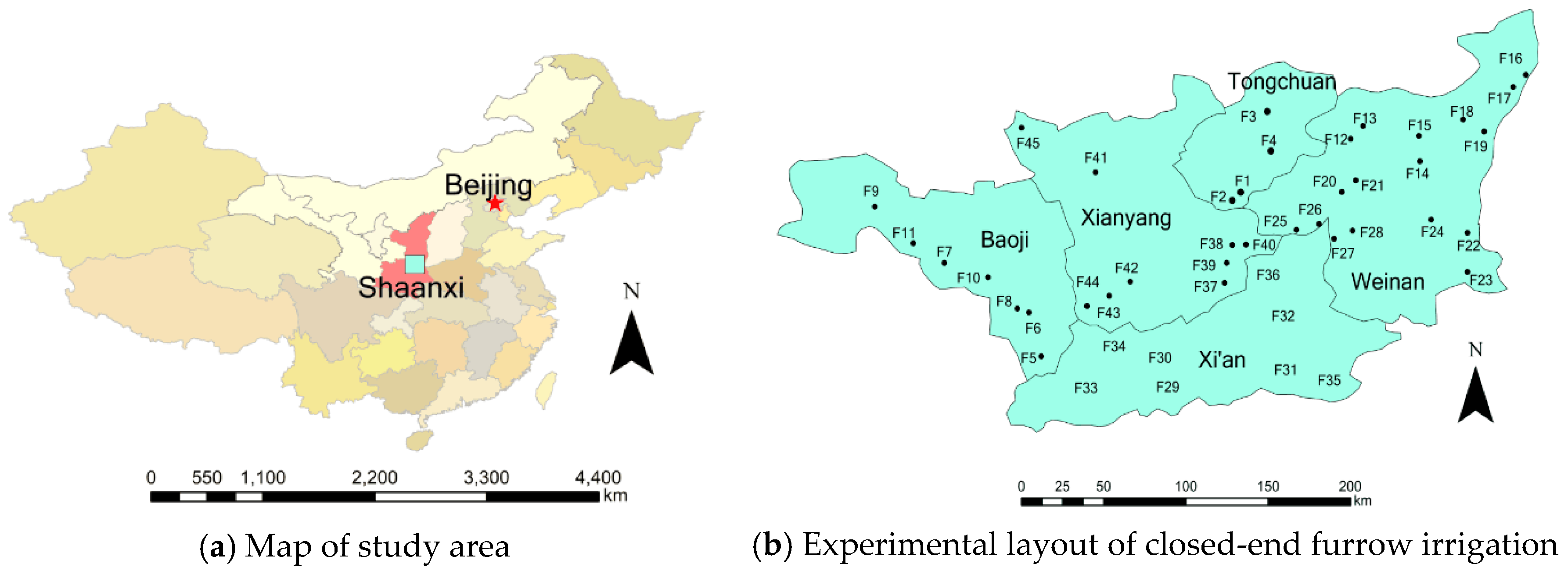
2.1. Experiments with Closed-End Furrow Irrigation

The Guanzhong plain is in the central part of Shaanxi Province, China, and it has an area of approximately 55,000 km2 and an elevation range of approximately 323–800 m. The annual average temperature is 12.8 °C, and the average annual precipitation is 605 mm. Combined with the actual irrigation experience of local farmers, closed-end furrow irrigation experiments were performed in the Guanzhong plain from July to August 2017, using planted crop maize. The study used 45 experimental sites with minimum and maximum longitudes of 106°55′57″ and 110°29′32″ N, and minimum and maximum latitudes of 33°49′26″ and 35°30′02″ E. The layout of the experimental sites is illustrated in Figure 1. At each experimental site, three to five furrows were laid out. The trapezoidal section most commonly used in northern China was adopted for these irrigation experiments. The downstream end of each furrow was closed, and the cutoff time was recorded when water reached the downstream end. The required water depth was 80 mm. The discharge was measured by a triangle weir. The measurement points were set at 10 m intervals along the furrow length (the last observation point was taken as the actual remaining length if the residual distance was within 10 m). The water advance time was recorded, and the water depths were measured every 1–5 min (every 1 min in the first 6 min, every 2 min from the sixth to the 10th min, and then every 5 min). One day before and one day after irrigation, five to eight measuring points were set along the furrow length. Each point was divided into five layers (i.e., 10, 20, 40, 60, and 80 cm) for soil water content collection, and two or three soil samples were selected at each measuring point to determine the bulk density of each layer. The soil was collected at four depth levels, namely 10, 20, 40, and 60 cm (it would have been difficult to collect soil samples at 80 cm; thus, the bulk density of the layer at 80 cm was assumed to be equal to that of the layer at 60 cm). The soil texture was classified according to the international reclassification standard (clay was ≤0.002 mm, silt was 0.002–0.02 mm, and sand was 0.02–2 mm). The detailed measurements of closed-end furrow irrigation at each experimental site are listed in Table 1 (these detailed measurements are the mean values for each experimental site). Because the opportunity time is relatively short for completing furrow irrigation, soil infiltration capacity mainly depends on the upper-layer soil properties. Therefore, the bulk density, initial soil water content, and soil particle proportions for each experimental site were recorded as mean values for soil layers from 0 to 40 cm (Table 1). These provided the basic values for PTF that were used to estimate the normalization factor.

2.2. SIPAR_ID and WinSRFR Descriptions

SIPAR_ID was proposed by Rodríguez and Martos in 2007, and it consists of a hybrid model that combines a volume balance principle with four artificial neural networks. It inverts the infiltration parameters and Manning’s roughness of surface irrigation by using a differential evolution method [35]. Because of the short length of the fields in northern China, which are mostly shorter than 200 m [41]—the maximum length of the furrow irrigation in this study was 130 m, as evident in Table 1—and a fairly short opportunity time (maximum opportunity time was 66 min), it was generally difficult to achieve stable infiltration, while estimation of the basic infiltration rate was challenging. Various studies have demonstrated that the Kostiakov equation achieves a high degree of precision in describing the soil infiltration process of surface irrigation [5,42,43,44,45]. Therefore, the Kostiakov equation was adopted to characterize the infiltration process of furrow irrigation; which can be written as:
Z = k τ α
where Z is the cumulative infiltration per unit area (mm), k is the infiltration coefficient (mm mina), α is the infiltration index, and τ is the opportunity time (min). The basic data concerning field length, bottom slope, cross-sectional parameters, inflow discharge, advance trajectory, and water depth in the upstream (an optional item) obtained through the field experiments were the inputs for SIPAR_ID, and the differences between simulated and measured values of advance trajectory were minimal. Thus, this was used as the objective function for estimating the infiltration parameters and Manning’s roughness. Note that, Furrow irrigation involves a two-dimensional infiltration (in lateral and vertical directions; i.e., simultaneous infiltration of both the width and depth of the furrow); in this study, the infiltration coefficient was obtained by SIPAR_ID as the inversion of the cumulative infiltration per unit length, which was divided by the furrow spacing (to match the infiltration characteristic item in a simulation of furrow irrigation by WinSRFR); that is, the infiltration coefficient k in Equation (1), under the cumulative infiltration per unit area [3,46]. Unlike conventional optimization, SIPAR_ID attempts to avoid most typical violations of the mass conservation principle. For example, volume balance methods use a uniform flow equation such as Manning’s equation to describe the cross-sectional area of flow at the field inlet, and then posit assumptions regarding the shape of the flow profile downstream. Typical volume balance methods generally assume that the cross-sectional area is constant, which is known to introduce substantial errors [35]. As the principle of volume balance is the basis of SIPAR_ID, the data used for estimating infiltration parameters and Manning’s roughness of the furrow irrigation comprise the advance trajectory and water depth, with no need for the data collection of recession trajectory, which is a hard work, and the practicability of the SIPAR_ID is then improved. However, it is difficult to fully account for the interaction between the infiltration parameters and Manning’s roughness during the inversion procedure [47]. Therefore, to verify the reliability of infiltration parameters and Manning’s roughness inversed by SIPAR_ID, the inversed results were input into WinSRFR for furrow irrigation simulation, and then the measured data were compared with the simulated advance trajectory and water depth.
WinSRFR, proposed by the USDA—Agricultural Research Service, is an integrated software package for analyzing surface irrigation systems. It consists of two models: the zero-inertia (ZI) model and the kinematic-wave model [41]. Closed-end furrows were used for maize in the aforementioned experiments; thus, the ZI model was selected to simulate the irrigation performance at each experimental site. The ZI model used in these procedures is as follows:
A t   +   q x   +   I t   = 0
h x   = S 0   S f
where A is the cross-sectional area of flow (m2), q is the discharge (m3 min−1), x is the distance from the field inlet (m), h is the water depth (m), t is time (min), S0 is the bottom slope of the furrow, Sf is the friction slope, and I is the unit length of infiltration volume (m3 m−1). Here, I is calculated from furrow spacing, which is the transverse width when infiltration is independent of the wetted perimeter, in the simulation of furrow irrigation by WinSRFR. Thus, Equation (1) is multiplied by the furrow spacing.

2.3. Influence of Manning’s Roughness on Advance Trajectory and Performance Indicators of Furrow Irrigation

To analyze the effect of Manning’s roughness on the water trajectory and irrigation performance for closed-end furrows, Manning’s roughness was input into WinSRFR in three simulation scenarios (henceforth, Sim.1, Sim.2, and Sim.3). For example, the Manning’s roughness cumulative frequency values were set at 5%, 50%, and 95% in Sim.1, Sim.2, and Sim.3, respectively. In addition, the other input parameters (i.e., furrow length, cross-section of the furrow, discharge, etc.) were the values measured at the experimental sites, as displayed in Table 1. The infiltration parameters and Manning’s roughness were adopted as the inverted results based on the advance trajectory and water depth of each experimental site; calculations were performed using SIPAR _ID.
The advance trajectory and performance of closed-end furrow irrigation were simulated in WinSRFR. The evaluative indicators of furrow irrigation performance usually include the application efficiency (Ea), the storage efficiency (Es) [12], and Christiansen’s uniformity (CU); CU indicates the uniformity distributed along the furrow length. The mathematical expressions for these indices are:
E a = Z s Z f
E s = Z s Z r
C U = 1 m = 1 N | Z m i Z ¯ i | N Z ¯ i
where Zs is the average depth of the infiltrated water stored in the root zone, Zf is the depth of total water applied (mm), Zr is the required water depth (all the Zr were set at 80 mm in this study), Zmi is the infiltrated depth of the m-th measurement point for the i-th furrow, Z ¯ i is the average depth of infiltration, and N is the number of measurement points. Note that Zs, Zmi, and Z ¯ i can be calculated from the soil water content and bulk density measured at multiple points along the length of the furrow one day before and after the irrigation. At least five measurement points (i.e., N) were set for soil water content along the length of each furrow.

2.4. Functional Normalization of the Kostiakov Equation and PTF Development

The scaling technique, which is extensively used to assess the variability of soil infiltration capacity, has been developed from similar theory. One of the theory-based soil infiltration models, the scaling process of the Philip model, was detailed by Machiwal et al. [24]. However, the Kostiakov equation, Equation (1) in this study, is an empirical equation, and parameters k and a do not have physical meanings; thus, the similarity theory method cannot be adopted. Analyzing soil infiltration capacity variability using multiple variables (k and a) is difficult because the two parameters are interactive. Therefore, the method introduced by Tillotson and Nielsen [48] can deal with functional normalization of the Kostiakov equation. Functional normalization aims to incorporate all infiltration relationships in the set into a single reference curve ( Z ¯ ). For each original infiltration curve, the normalization factor (FC) is calculated from the following equation:
F C i = j = 1 M Z i j Z ¯ j M = j = 1 M k i τ j α i k ¯ τ j a ¯ M
where FCi is the calculated normalization factor for the i-th furrow, Zij is the cumulative infiltration from Equation (1) for the i-th furrow, Z ¯ j is the average cumulative infiltration of j-th opportunity time for all furrows, and M is the sequence number of opportunity time. Then, Z ¯ can be written as:
Z ¯ = k ¯ τ a ¯
where k ¯ and α ¯ are the average infiltration parameters for all furrow irrigation experiments. Substituting Equations (7) and (8) into Equation (1), the infiltration property of an arbitrary furrow can be described by:
Z = F C Z ¯ = F C k ¯ τ a ¯
Because the soil infiltration parameters of each experimental site were obtained through the estimation of the advance trajectory, the opportunity time of each experimental site was quite different in the FC calculations. Therefore, the maximum advance time was considered for the furrow irrigation (i.e., F23 with 66 min (Table 1) as a basis) and all opportunity times were adjusted to 70 min in this study. To develop PTF in MATLAB, multiple linear regression analyses were applied to correlate FC with available soil physical parameters (i.e., soil particle proportions, bulk density, and initial soil water content), which were based on the results of a correlation analysis run in SPSS.

2.5. Optimization of Inflow Discharge Based on Manning’s Roughness Representative Values and PTF to Estimate the Mean Infiltration Parameters

To generate an easy-to-use and practical method for the design and management of furrow irrigation systems at regional scales, optimal inflow discharge values were determined through two additional simulation runs of different simulation scenarios (henceforth, Sim.4 and Sim.5) in WinSRFR; these were defined as follows. In Sim.4, field mean infiltration parameters and Manning’s roughness for each furrow were inverted by SPAIR_ID (representing the actual field situation of the furrow irrigation), and in Sim.5, field mean infiltration parameters were determined by the PTF of each furrow and the Manning’s roughness cumulative frequency as 50% (representing the adopted strategy of Manning’s roughness and field mean infiltration parameters in the proposed method).
The other input parameters were adopted from the values measured at the experimental sites, as displayed in Table 1. Considering that the bottom slopes and lengths of the actual furrow fields were variable at a regional scale, to make the research results robust, various combinations of bottom slope and length were selected. The furrow bottom slopes were 0.001, 0.0025, and 0.004; the furrow lengths were 80, 105, and 130 m. The required water depth was 80 mm, the furrow bottom width was 0.23 m, the furrow depth was 0.15 m, the side slope was 0.7, and the furrow spacing was 0.65 m. To determine the optimal discharge, the discharges of each furrow were set at 2.0, 3.0, 4.0, 5.0, and 6.0 L s−1.
An equation similar to that of Wang et al. [49], in which the maximum geometric mean value is adopted as an evaluation indicator for closed-end furrow irrigation performance, can be written as follows:
Y = E a × E s × C U 3
where Y is the comprehensive performance indicator of closed-end furrow irrigation. In numerous studies, the adopted cutoff time in furrow irrigation is the moment of completion of the advance phase [50], and farmers in northern China typically set the cutoff time at the moment that the water reaches the downstream end [41,51]. In furrow irrigation, selecting an appropriate discharge is more robust than the approach of limiting length and cutoff time, particularly when a farmer has poor control over the water [16]. Therefore, for practical purposes, the cutoff time in this study was defined as the time at which the water reached the downstream end; this definition yielded reasonable discharge values.

2.6. Criteria for Evaluation

In this study, the performance of the simulated results was evaluated by comparing the statistical indicator of the simulated values with the measured values. The indicator used was mean absolute percent relative error (MAPRE); it can be calculated as follows [52]:
MAPRE = 1 W f = 1 W ( | X s f X m f | X m f × 100 % )
where f is an integer varying from 1 to W; W is the total number of data sets; Xsf is the f-th simulated value; Xmf is the f-th measured or simulated value (the simulation results of Sim.4 served as a benchmark). Note that, in the PTF estimations, Xsf represents the estimated PTF results and Xmf represents the results of Equation (7). MAPRE enables a quantitative comparison of the simulated values with the measured values for the advance trajectory of furrow irrigation, indicators of irrigation performance, and normalization factor FC. MAPRE is a measure of the accuracy of the models with the simulated and measured values, and low values of MAPRE indicate a favorable simulation accuracy [53].

3. Results and Discussion

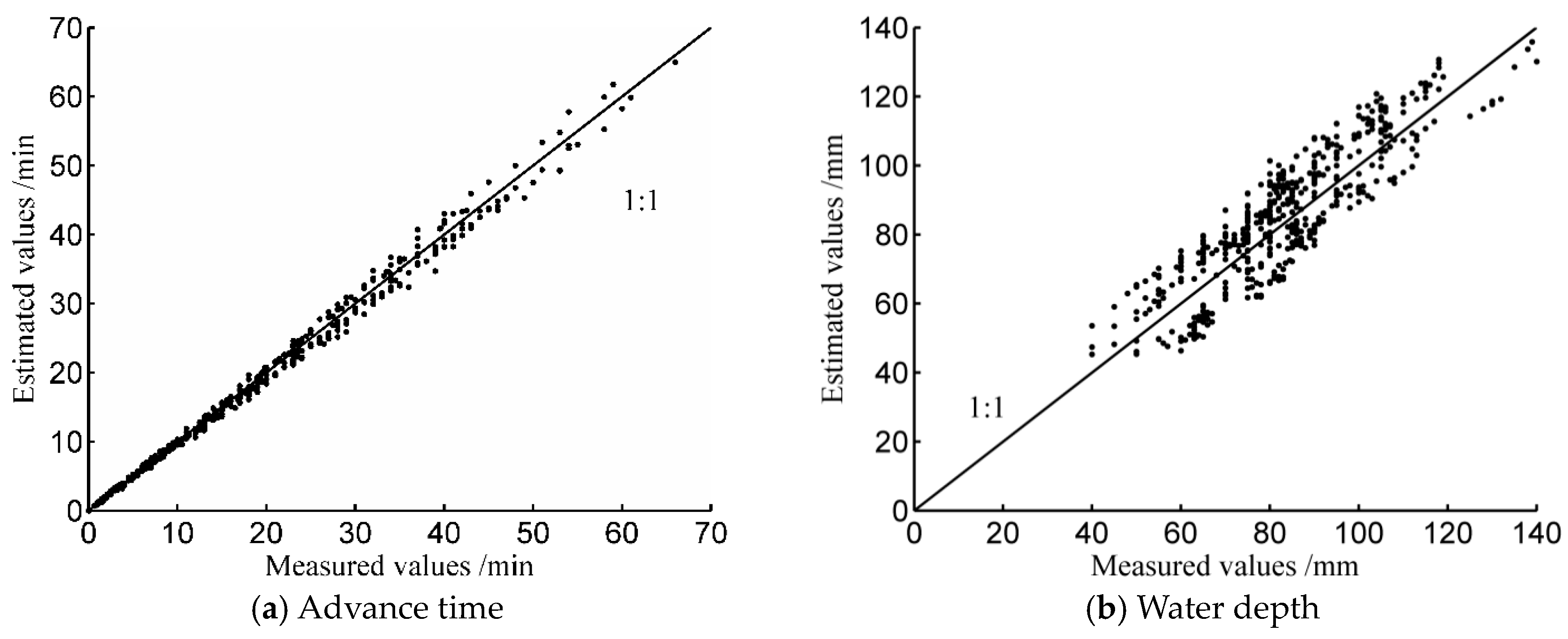
3.1. Reliability Analysis of Field Mean Infiltration Parameters and Manning’s Roughness

Field mean infiltration parameters and Manning’s roughness values were estimated using SIPAR_ID. The results are listed in Table 2, and they prove that field mean infiltration parameters and Manning’s roughness were different for each experimental site. The reasons were that the cross-sectional area (or wetted perimeter) varied with different inflow discharges, and that the variability of soil characteristics at the field scale caused differences in field mean infiltration parameters and Manning’s roughness values for each experimental site.
Here, the accuracy of field mean infiltration parameters and Manning’s roughness values estimated using SIPAR_ID were considered closely. The estimated values (Table 2) were entered into WinSRFR, and the advance trajectory and water depths in the upstream were simulated for each furrow experiment to ensure the reliability of the estimated parameters. Then, the simulated values were compared with the measured values, as presented in Figure 2 and Table 2. The results proved that WinSRFR simulations of water advance trajectories were in good agreement with the measured data. The MAPRE of advance time (between measured and simulated values) was 4.8% for all furrow irrigation experiments. The simulated and measured water depth values in the upstream exhibited acceptable agreements, yielding a MAPRE of 10.8%. Possibly, the water depth was not steady enough in the upstream or during the furrow irrigation. The maximum flow velocity tended to be realized close to the inlet; therefore, soil erosion may be greater at the forehead than at the following segments along the furrow [54], and this tends to promote uncertainty for water depth in the measurement process. However, in the context of actual furrow irrigation projects, the error of water depth between the measured and simulated values was within a reasonable range. Therefore, the field mean infiltration parameters and Manning’s roughness values estimated with SIPAR_ID were reliable.

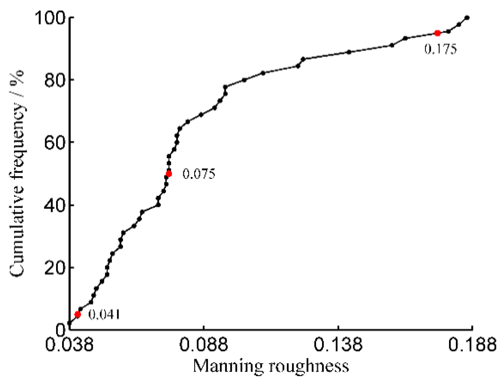
3.2. Evaluation of the Influence of Manning’s Roughness on Advance Trajectory and Irrigation Performance, and the Determination of its Representative Value in a Maize Field

As presented in Figure 3, the Manning’s roughness values of Sim.1, Sim.2, and Sim.3 were 0.041 (cumulative frequency, 5%), 0.075 (cumulative frequency, 50%), and 0.175 (cumulative frequency, 95%), respectively. The advance trajectory and irrigation performance under the first three simulation scenarios (Sim.1, Sim.2, and Sim.3) were simulated using WinSRFR. Then, the simulated advance time and irrigation performance indicators were compared with the measured values, and the results are presented in Figure 4.
The MAPREs of advance time between the measured and simulated values for all furrow irrigation experiments under Sim.1, Sim.2, and Sim.3 were 10.5%, 6.7%, and 10.2%, respectively (Figure 4(a1)–(a3)). The results proved that the simulated advance times were slightly underestimated relative to the measured values under Sim.1 and slightly overestimated under Sim.3; the greatest consistency between the measured and simulated values occurred under Sim.2. The Manning’s roughness of Sim.1 was 0.041, which was less than the roughness values of most furrow irrigation experiments (Figure 3); a small roughness value may increase flow velocity, resulting in an underestimation of advance time. However, the Manning’s roughness of Sim.3 was 0.175, which was much greater than the values of most furrow irrigation experiments (Figure 3), and the excessive values may reduce the flow velocity, resulting in an overestimation of the advance time. Sim.2, with a Manning’s roughness of 0.075, accurately represented the roughness values of most furrow irrigation experiments (close to the average value of 0.085, Table 2); thus, Sim.2 demonstrated the best consistency between simulated values and measured values.
The simulated irrigation performance indicators generated by WinSRFR were in agreement with the measured values (Figure 4(b1)–(b3)). The MAPRE values of Ea, CU, and Es between the measured and simulated values for all furrow irrigation experiments under Sim.1 were 8.3%, 3.9%, and 4.8%, respectively. Only small differences were evident between the simulated and measured values of irrigation performance under Sim.2. Compared with Sim.1, the MAPRE values of Ea, CU, and Es under Sim.2 were decreased by 3.4%, 1.7%, and 3.0%, respectively. For Sim.3, the MAPRE values, between the measured and simulated values, were 9.4%, 4.6%, and 2.5%. The typical Manning’s roughness value for the maize fields in this study was 0.075. In general, the advance trajectory and irrigation performance indicators were not sensitive to variations in Manning’s roughness, which can be used as a representative value (i.e., 0.075) in a maize field to simulate the advance trajectory and irrigation performance of a closed-end furrow.

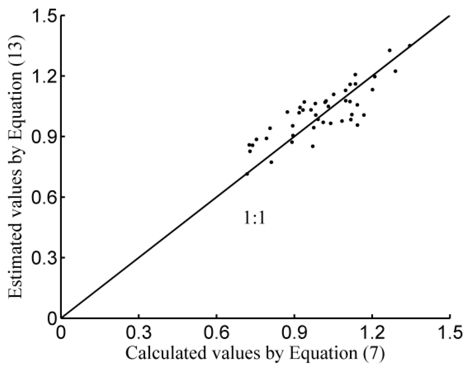
3.3. Establishment of the Normalization Function and PTF and Verification

The mean values of the infiltration parameters (Table 2) were put into Equation (9). The normalization function of the study area can be written as:
Z = 113.68 F C τ 0.485
Here, the accuracy of the infiltrated depth estimated with Equation (12) was emphasized. The values of FC for each experimental site were calculated with Equation (7); the results are listed in Table 2. Then, FC was put into Equation (12) to obtain the estimated infiltration depths, which can be compared with the values calculated from the infiltration parameters in Table 2. The results are presented in Figure 5.
As illustrated in Figure 5, the infiltration depths estimated using Equation (12) were in good agreement with the values calculated from the infiltration parameters in Table 2, and the regression lines were notably close to the 1:1 line. The coefficient of determination (R2) from the regression was 0.95, and the MAPRE was 7.3% for all furrow irrigation experiments. The relatively high R2 and relatively low MAPRE indicated the high accuracy achieved using Equation (12) for estimating the infiltration depth, and the reasonable functional normalization of the Kostiakov equation.
SPSS was applied to analyze the correlations between FC and soil particle proportions, soil bulk density (γd), and initial soil water content (θ0). The results indicated that the variability of FC was related mainly to sand content (Sa), clay content (Cl), soil bulk density, and initial soil water content; the correlation coefficients were 0.79, −0.73, −0.61, and −0.59 in the study area. However, FC was not significantly related to silt content, which had a correlation coefficient of −0.19. To develop PTF, multiple linear regression analyses were conducted in MATLAB on the basis of correlation analysis. In the study area, the PTF can be represented as:
F E = 1.68 0.80 × C l + 1.80 × S a 0.75 × γ d 0.80 × θ 0
where Cl is the clay content (%), Sa is the sand content (%), γd is the soil bulk density (g cm3), and θ0 is the initial soil water content (%). The γd, θ0, Cl, and Sa terms in Equation (13) were set to the mean values of the 0–40 cm soil layers measured at each experimental site. To ensure reliability, the FE estimates from Equation (13) were compared with the values of FC calculated using Equation (7). As illustrated in Figure 6, the estimated FE values were comparatively consistent with the calculated values, and the regression lines were notably close to the 1:1 line (Figure 6). The R2 and the MAPRE values were 0.56 and 7.7% in the study area, respectively. The results demonstrated that using Equation (13) to estimate FC generated reliable results in the study area.

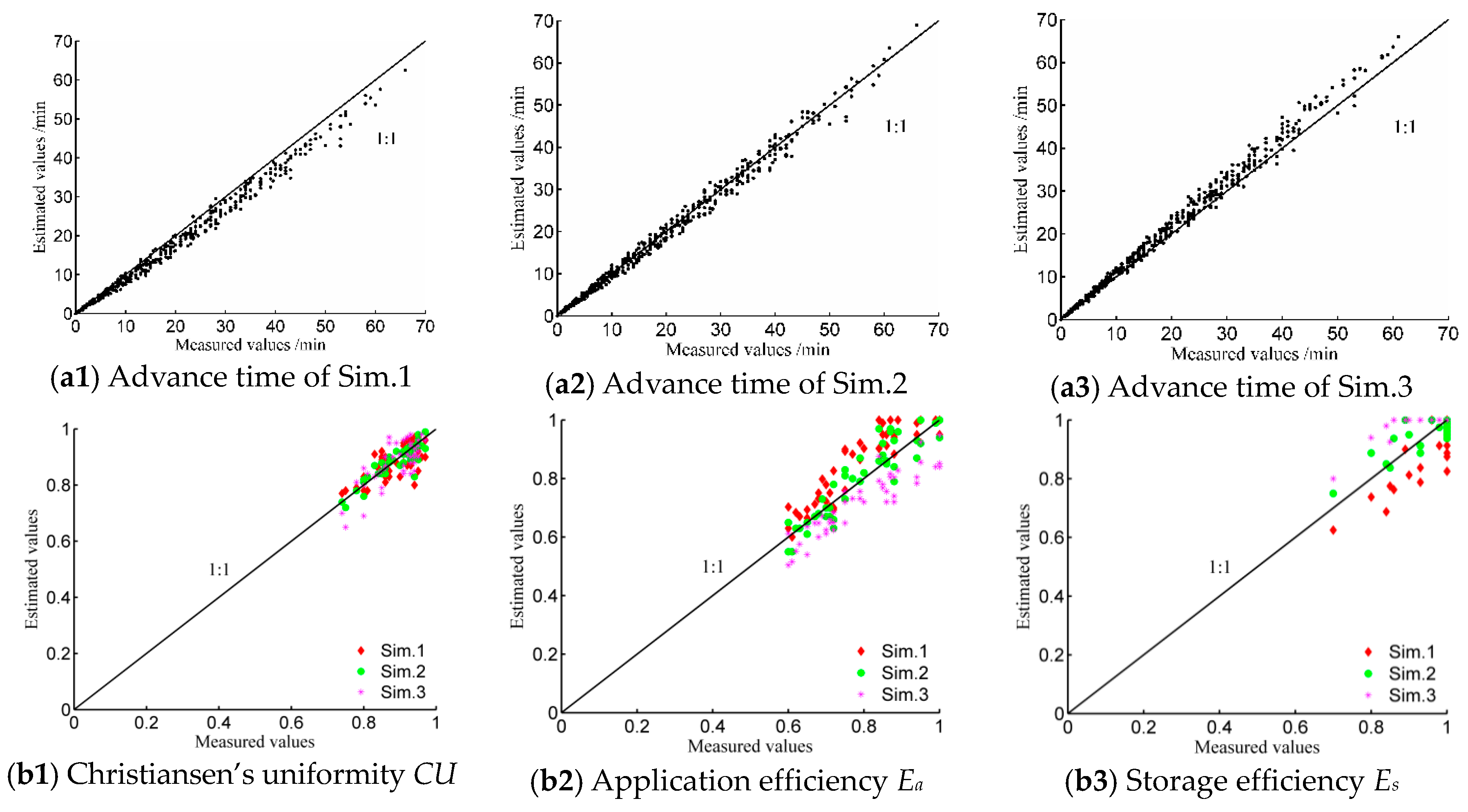
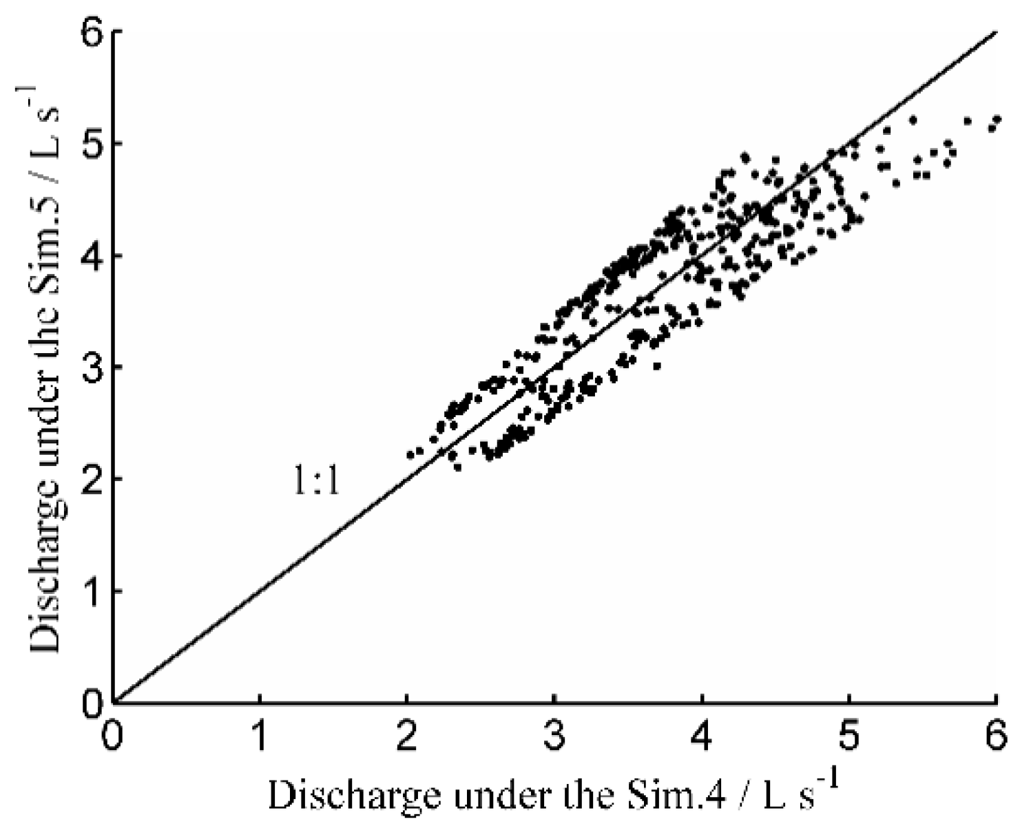
3.4. Reliability Verification of the Proposed Method for Determining the Inflow Discharge at a Regional Scale

The irrigation performance indicators (Ea, CU, and Es) were simulated using WinSRFR under Sim.4 and Sim.5, and then the comprehensive indicator Y was estimated using Equation (10). In the WinSRFR simulations, the furrow bottom slopes were 0.001, 0.0025, and 0.004, the furrow lengths were 80, 105, and 130 m, and the discharges were 2.0, 3.0, 4.0, 5.0, and 6.0 L m−1; a total of 2025 simulations were run for all furrow irrigation sites under Sim.4 and Sim.5.
The comprehensive indicator, Y, of closed-end furrow irrigation performance exhibited an increasing trend, and then a decreasing trend as the discharge increased, which was consistent with a second-order parabolic equation for furrows with the same length and bottom slope. Solving the fitted second-order parabolic equation yielded the optimal discharge for each experimental site in both Sim.4 and Sim.5. The optimal discharges were compared between Sim.4 and Sim.5, and the results are presented in Figure 7.
The optimal discharge of each experimental site was approximately the same in Sim.4 and Sim.5 (Figure 7). The R2 was 0.76 for all experimental sites. The MAPRE of optimal discharge between Sim.4 and Sim.5 for all furrow irrigation experiments was 9.2%; the simulation results of Sim.4 served as a benchmark. From the optimal results of discharge depicted in Figure 7, the irrigation performance indicators were estimated using WinSRFR, and then the comprehensive indicator, Y, was obtained according to Equation (10). The results are displayed in Table 3.
The simulated indicators based on the optimized discharge were different (Table 3), but the differences were relatively small. The minimum, maximum, and mean values of the comprehensive indicator, Y, were basically consistent under various bottom slope and furrow length combinations in Sim.4 and Sim.5. The mean values with small variation coefficients, and the comprehensive indicators of irrigation performance were greater than 0.80. This finding indicated that the irrigation performance levels were not sensitive to variations of Manning’s roughness. In this study, a Manning’s roughness value of 0.075 represented the performance of a closed-end irrigation furrow in maize fields. The results also demonstrated that the PTF were able to estimate the normalization factors FC, and that it could be used for determining the optimized discharge of closed-end furrow irrigation of maize fields in the study areas. A properly optimized design can ensure high irrigation performance.

3.5. General Discussion

The Manning’s roughness values presented in Table 2 had a wide range, 0.038–0.186, and the maximum value (0.186 in F15) was approximately five times that of the minimum value (0.038 in F6). The causes were as follows: first, in some furrows (i.e., F1, F11, F15, F35, F39, and F45), the bottoms were unsmoothed, and many clods in the side slopes had been manually excavated. Second, the accuracy of estimation depended on the accuracy of the data regarding upstream water depth; SIPAR_ID was used to estimate the field mean infiltration parameters and Manning’s roughness. Last, in the inversion procedure for infiltration parameters and Manning’s roughness, it was difficult to fully consider the interactive influence between parameters because of the uncollected data concerning the recession trajectories, which may lead to overestimation/underestimation of Manning’s roughness in some irrigation furrows. The simulated values of the advance time and performance indicators had a slight influence when the various Manning’s roughness values (0.041, 0.075, and 0.175) were adopted (Figure 4), indicating that the advance trajectory and performance indicators of closed-end furrow irrigation were not sensitive to variations of Manning’s roughness. This result was similar to the results of Smith et al. [2], Salahou et al. [5], and Nie et al. [19]. These findings indicate that the Manning roughness of maize field can be used as a representative value (i.e., 0.075, 50% of the cumulative frequency of all experimental sites) to simulate the advance trajectory and irrigation performance of a closed-end furrow.
The soil infiltration capacity variability was represented by variability in k; α was constant in Equation (1), which was normalized by the methods of Jaynes and Clemmens [55], Oyonarte et al. [56], and Nie et al. [18]. A similar method was used to predict the mean infiltration for each furrow and a whole field, based on the volume balance principle of Khatri et al. [57], and a satisfactory result was obtained because the scaled infiltration curves had shapes similar to those of the actual curves. Bai et al. [58] described infiltrations at 66 sites, and determined that the distribution of infiltrated depth was significantly correlated to that of k, but it was not significantly correlated to that of α. Although the coefficient of variation (CV) of k was 0.18 (Table 2), which was smaller than the CV of a (0.36), the method of normalization of the Kostiakov equation was adopted in this study. The infiltrated depths estimated using Equation (12) were in close agreement with the values calculated from the field mean infiltration parameters in Table 2 (Figure 5), which proved that the normalization method was feasible for the Kostiakov equation. Table 2 indicates that the CV of the normalization factor, FC, in this study area was 0.156; however, in 72 double-ring infiltration experiments in the typical fields of the first and third terraces (Yangling, Shaanxi province, China), the values of CV of FC were 0.334 and 0.271 [40]. The results demonstrated that the variability may be overestimated by point infiltration measurement, which obtained results similar to those of Bautista and Wallender [28]. Therefore, it can be inferred that using the field mean infiltration parameters may be helpful for obtaining a more robust design of a furrow irrigation system and managing such an irrigation system.
The proposed method of this study for determining the optimal discharge only required information regarding the soil particle proportions, bulk density, and initial soil water content in 0–40 cm soil layers, which were relatively steady and easy to obtain at a regional scale. Therefore, the system provided a practical and convenient method for optimizing the discharge of closed-end furrow irrigation. Only two soil textures (loamy clay and clay loam) were considered in this study; other soil textures require further verification. The PTF presented in this study might only be suitable and reasonable in the study area, but the research method could provide a reference for optimizing the discharges of closed-end furrow irrigation in other regions.

4. Conclusions

(1) The influences of Manning’s roughness on advance trajectory and irrigation performance were evaluated. The results demonstrated that the advance trajectory and irrigation performance indicators were not sensitive to variations in Manning’s roughness; the Manning’s roughness value in the present study can be used as a representative value (i.e., 0.075) for typical maize fields to simulate closed-end furrow irrigation.
(2) The normalization method was proven to be feasible for the Kostiakov equation. The PTF, which can be used to estimate the normalization factors, were established and verified. The PTF were established on the basis of the results of correlation analysis. The normalization factors estimated by PTF were compared with calculated values, and the MAPRE was 7.7%, which demonstrated that the PTF for estimating the normalization factor were reliable in the study area.
(3) The discharge of closed-end furrow irrigation was determined from representative values of Manning’s roughness and field mean infiltration parameters that were estimated with regional-scale PTF. The results indicated that under various combinations of furrow length and bottom slope, the optimal inflow discharge determined by the proposed method was basically consistent with the discharge that was determined by inverted infiltration parameters and Manning’s roughness using SIPAR_ID, which proved the proposed method was reliable and can be used to obtain superior irrigation performance. It also provided an easy, practical method for evaluating the design and management of closed-end furrow irrigation systems.

Author Contributions

W.-B.N., Y.-B.L., and X.-Y.M. analyzed the data; W.-B.N. and Y.-B.L. wrote the paper; F.Z., S.-X.D., and H.W. conducted the furrow irrigation experiments.

Funding

This research was funded by grants from the National Program on Key Research Projects during the 13th Five-Year Plan Period (2016YFC0400203), National Natural Science Foundation of China (No. 51579205 and No. 51279167), and the Special Fund for Agro-Scientific Research in the Public Interest (No. 201503124).

Conflicts of Interest

The authors declare no conflict of interest.

References

  1. Akbari, M.; Gheysari, M.; Mostafazadeh-Fard, B.; Shayannejad, M. Surface irrigation simulation-optimization model based on meta-heuristic algorithms. Agric. Water Manag. 2018, 201, 46–57. [Google Scholar] [CrossRef]
  2. Smith, R.J.; Uddin, M.J.; Gillies, M.H. Estimating irrigation duration for high performance furrow irrigation on cracking clay soils. Agric. Water Manag. 2018, 206, 78–85. [Google Scholar] [CrossRef]
  3. Bautista, E.; Clemmens, A.J.; Strelkoff, T.S.; Schlegel, J. Modern analysis of surface irrigation systems with WinSRFR. Agric. Water Manag. 2009, 96, 1146–1154. [Google Scholar] [CrossRef]
  4. Gillies, M.H.; Smith, R.J. SISCO—Surface irrigation simulation calibration and optimisation. Irrig. Sci. 2015, 33, 339–355. [Google Scholar] [CrossRef]
  5. Salahou, M.K.; Jiao, X.Y.; Lü, H.S. Border irrigation performance with distance-based cut-off. Agric. Water Manag. 2018, 201, 27–37. [Google Scholar] [CrossRef]
  6. Miao, Q.F.; Shi, H.B.; Goncalves, J.M.; Pereira, L.S. Field assessment of basin irrigation performance and water saving in Hetao, Yellow River basin: Issues to support irrigation systems modernization. Biosyst. Eng. 2015, 136, 102–116. [Google Scholar] [CrossRef]
  7. Strelkoff, T.S.; Clemmens, A.J.; Bautista, E. Estimation of soil and crop hydraulic properties. J. Irrig. Drain. Eng. ASCE 2009, 135, 537–555. [Google Scholar] [CrossRef]
  8. Bautista, E.; Clemmens, A.J.; Strelkoff, T.S. Structured application of the two-point method for the estimation of infiltration parameters in surface irrigation. J. Irrig. Drain. Eng. ASCE 2009, 135, 566–578. [Google Scholar] [CrossRef]
  9. Chow, V.T. Open Channel Hydraulics; McGraw-Hill: New York, NY, USA, 1959. [Google Scholar]
  10. Li, Z.; Zhang, J. Calculation of field Manning’s roughness coefficient. Agric. Water Manag. 2001, 49, 46–57. [Google Scholar] [CrossRef]
  11. Zhang, S.H.; Xu, D.; Li, Y.N.; Cai, L.G. An optimized inverse model used to estimate Kostiakov infiltration parameters and Manning’s roughness coefficient based on SGA and SRFR model: (I) establishment. J. Hydraul. Eng. 2006, 37, 1297–1302. (In Chinese) [Google Scholar]
  12. Bautista, E.; Clemmens, A.J.; Strelkoff, T.S.; Niblack, M. Analysis of surface irrigation systems with WinSRFR—Example application. Agric. Water Manag. 2009, 96, 1162–1169. [Google Scholar] [CrossRef]
  13. Anwar, A.A.; Ahmad, W.; Bhatti, M.T.; Ul Haq, Z. The potential of precision surface irrigation in the Indus basin irrigation system. Irrig. Sci. 2016, 34, 379–396. [Google Scholar] [CrossRef]
  14. Eldeiry, A.; García, L.; Ei-Zaher, A.S.A.; Kiwan, M.E. Furrow irrigation system design for clay soils in arid regions. Appl. Eng. Agric. 2005, 21, 411–420. [Google Scholar] [CrossRef]
  15. Sánchez, C.A.; Zerihun, D.; Farrell-Poe, K.L. Management guidelines for efficient irrigation of vegetables using closed-end level furrows. Agric. Water Manag. 2009, 96, 43–52. [Google Scholar] [CrossRef]
  16. Reddy, M.; Jumaboev, K.; Matyakubov, B.; Eshmuratov, D. Evaluation of furrow irrigation practices in Fergana Valley of Uzbekistan. Agric. Water Manag. 2013, 117, 133–144. [Google Scholar] [CrossRef]
  17. Morris, M.R.; Hussaina, A.; Gillies, M.H.; O’Halloran, N.J. Inflow rate and border irrigation performance. Agric. Water Manag. 2015, 155, 76–86. [Google Scholar] [CrossRef]
  18. Nie, W.B.; Huang, H.; Ma, X.Y.; Fei, L.J. Evaluation of closed-end border irrigation accounting for soil infiltration variability. J. Irrig. Drain. Eng. ASCE 2017, 143. [Google Scholar] [CrossRef]
  19. Nie, W.B.; Fei, L.J.; Ma, X.Y. Impact of infiltration parameters and Manning roughness on the advance trajectory and irrigation performance for closed-end furrows. Span. J. Agric. Res. 2014, 12, 1180–1191. [Google Scholar] [CrossRef]
  20. Gillies, M.H. Managing the Effect of Infiltration Variability on the Performance of Surface Irrigation. Ph.D. Thesis, University of Southern Queensland, Toowoomba, Queensland, Australia, 2008. [Google Scholar]
  21. Duan, R.; Fedler, C.B.; Borrelli, J. Field evaluation of infiltration models in lawn soils. Irrig. Sci. 2011, 29, 379–389. [Google Scholar] [CrossRef]
  22. Tarboton, K.C.; Wallender, W.W. Field-wide furrow infiltration variability. Trans. ASAE 1989, 32, 913–918. [Google Scholar] [CrossRef]
  23. Schwankl, L.J.; Raghuwanshi, N.S.; Wallender, W.W. Furrow irrigation performance under spatially varying conditions. J. Irrig. Drain. Eng. ASCE 2000, 126, 355–361. [Google Scholar] [CrossRef]
  24. Machiwal, D.; Jha, M.K.; Mal, B.C. Modelling infiltration and quantifying spatial soil variability in a wasteland of Kharagpur, India. Biosyst. Eng. 2006, 95, 569–582. [Google Scholar] [CrossRef]
  25. Zapata, N.; Playán, E. Elevation and infiltration in a level basin. I. Characterizing variability. Irrig. Sci. 2018, 19, 155–164. [Google Scholar] [CrossRef]
  26. Zeleke, T.B.; Si, B.C. Characterizing scale-dependent spatial relationships between soil properties using multifractal techniques. Geoderma 2006, 134, 440–452. [Google Scholar] [CrossRef]
  27. Mubarak, I.; Jaramillo, R.A.; Mailhol, J.C.; Ruelle, P.; Khaledian, M.; Vauclin, M. Spatial analysis of soil surface hydraulic properties: Is infiltration method dependent? Agric. Water Manag. 2010, 97, 1517–1526. [Google Scholar] [CrossRef]
  28. Bautista, E.; Wallender, W.W. Spatial variability of infiltration in furrows. Trans. ASAE 1985, 28, 1846–1851. [Google Scholar] [CrossRef]
  29. Playán, E.; Rodriguez, J.A.; García-Navarro, P. Simulation model for level furrows. I: Analysis of field experiments. J. Irrig. Drain. Eng. ASCE 2004, 130, 106–112. [Google Scholar] [CrossRef]
  30. Khatri, K.L.; Smith, R.J. Toward a simple real-time control system for efficient management of furrow irrigation. Irrig. Drain. 2007, 56, 463–475. [Google Scholar] [CrossRef] [Green Version]
  31. Uddin, J.; Smith, R.J.; Gillies, M.H.; Moller, P.; Robson, D. Smart automated furrow irrigation of cotton. J. Irrig. Drain. Eng. ASCE 2018, 144. [Google Scholar] [CrossRef]
  32. Walk, W.R. Multilevel calibration of furrow infiltration and roughness. J. Irrig. Drain. Eng. ASCE 2005, 131, 129–136. [Google Scholar] [CrossRef]
  33. Nie, W.B.; Fei, L.J.; Ma, X.Y. Estimated infiltration parameters and manning roughness in border irrigation. Irrig. Drain. 2012, 61, 231–239. [Google Scholar]
  34. Philip, J.R. The theory of infiltration: 1. The infiltration equation and its solution. Soil Sci. 1957, 83, 345–357. [Google Scholar] [CrossRef]
  35. Rodríguez, J.A.; Martos, J.C. SIPAR_ID: Freeware for surface irrigation parameter identification. Environ. Model. Softw. 2010, 25, 1487–1488. [Google Scholar] [CrossRef]
  36. Etedail, H.R.; Ebrahimian, H.; Abbasi, F.; Liaghat, A. Evaluating models for the estimation of furrow irrigation infiltration and roughness. Span. J. Agric. Res. 2011, 9, 641–649. [Google Scholar] [Green Version]
  37. Kamali, P.; Ebrahimian, H.; Parsinejad, M. Estimation of Manning roughness coefficient for vegetated furrows. Irrig. Sci. 2018. [Google Scholar] [CrossRef]
  38. Wosten, J.H.M.; van Genuchten, M.T. Using texture and other soil properties to predict the unsaturated soil hydraulic functions. Soil Sci. Soc. Am. J. 1988, 52, 1762–1770. [Google Scholar] [CrossRef]
  39. Ghorbani, D.S.H.; Mahdi, H. Estimating soil water infiltration parameters using pedotransfer functions. Int. Assoc. Sci. Hydro. Bull. 2015, 61, 1477–1488. [Google Scholar] [CrossRef]
  40. Nie, W.B.; Ma, X.Y.; Fei, L.J. Evaluation of infiltration models and variability of soil infiltration properties at multiple scales. Irrig. Drain. 2017, 66, 589–599. [Google Scholar] [CrossRef]
  41. Chen, B.; Ouyang, Z.; Sun, Z.; Wu, L.; Li, F. Evaluation on the potential of improving border irrigation performance through border dimensions optimization: A case study on the irrigation districts along the lower Yellow River. Irrig. Sci. 2013, 31, 715–728. [Google Scholar] [CrossRef]
  42. Alvarez, J.A.R. Estimation of advance and infiltration equations in furrow irrigation for untested discharges. Agric. Water Manag. 2003, 60, 227–239. [Google Scholar] [CrossRef]
  43. Amer, A.M. Effects of water infiltration and storage in cultivated soil on surface irrigation. Agric. Water Manag. 2011, 98, 815–822. [Google Scholar] [CrossRef]
  44. Burguete, J.; Zapata, N.; García-Navarro, P.; Maïkaka, M.; Playán, E.; Murillo, J. Fertigation in furrows and level furrow systems. I: Model description and numerical tests. J. Irrig. Drain. Eng. ASCE 2009, 135, 401–412. [Google Scholar] [CrossRef]
  45. Holzapfel, E.A.; Jara, J.; Zuniga, C.; Marino, M.A.; Paredes, J.; Billib, M. Infiltration parameters for furrow irrigation. Agric. Water Manag. 2004, 68, 19–32. [Google Scholar] [CrossRef]
  46. Bautista, E. Effect of infiltration modeling approach on operational solutions for furrow irrigation. J. Irrig. Drain. Eng. ASCE 2016, 142. [Google Scholar] [CrossRef]
  47. Katopodes, N.D.; Tang, J.H.; Clemmens, A.J. Estimation of surface irrigation parameters. J. Irrig. Drain. Eng. ASCE 1990, 116, 676–696. [Google Scholar] [CrossRef]
  48. Tillotson, P.M.; Nielsen, D.R. Scale factors in soil science. Soil Sci. Soc. Am. J. 1984, 48, 953–959. [Google Scholar] [CrossRef]
  49. Wang, W.H.; Jiao, X.Y.; Peng, S.Z.; Chen, X.D. Sensitivity analysis of border irrigation performance using robust design theory. Trans. CSAE 2010, 26, 37–42. (In Chinese) [Google Scholar]
  50. Wattenburger, P.L.; Clyma, W. Level basin design and management in the absence of water control. Part I: Evaluation of completion-of-advance irrigation. Trans. ASAE 1989, 32, 838–843. [Google Scholar] [CrossRef]
  51. Pereira, L.S.; Goncalves, J.M.; Dong, B.; Mao, Z.; Fang, S.X. Assessing basin irrigation and scheduling strategies for saving irrigation water and controlling salinity in the upper Yellow River Basin, China. Agric. Water Manag. 2007, 93, 109–122. [Google Scholar] [CrossRef]
  52. Moriasi, D.; Arnold, J.; Liew, M.W.V.; Veith, T.L. Model evaluation guidelines for systematic quantification of accuracy in watershed simulations. Trans. ASABE 2007, 50, 885–900. [Google Scholar] [CrossRef]
  53. Jacovides, C.P.; Kontoyiannis, H. Statistical procedures for the evaluation of evapotranspiration computing models. Agric. Water Manag. 1995, 27, 365–371. [Google Scholar] [CrossRef]
  54. Trout, T.J. Furrow irrigation erosion and sedimentation: On-field distribution. Trans. ASAE 1996, 39, 1717–1723. [Google Scholar] [CrossRef]
  55. Jaynes, D.B.; Clemmens, A.J. Accounting for spatially variable infiltration in border irrigation models. Water Resour. Res. 1986, 22, 1257–1262. [Google Scholar] [CrossRef]
  56. Oyonarte, N.A.; Mateos, L.; Palomo, M.J. Infiltration variability in furrow irrigation. J. Irrig. Drain. Eng. ASCE 2002, 128, 26–33. [Google Scholar] [CrossRef]
  57. Khatri, K.L.; Smith, R.J. Real-time prediction of soil infiltration characteristics for the management of furrow irrigation. Irrig. Sci. 2006, 25, 33–43. [Google Scholar] [CrossRef]
  58. Bai, M.J.; Xu, D.; Li, Y.N.; Li, J.S. Evaluating spatial and temporal variability of infiltration on field-scale under surface irrigation. J. Soil Water Conserv. 2005, 19, 120–123. (In Chinese) [Google Scholar]
Figure 1. Map of study area and experimental layout of closed-end furrow irrigation. Notes: represents the study area. ● represents an experimental site.
Water 10 01825 g001
Figure 2. Comparisons of measured and simulated advance time and water depth in the upstream using WinSRFR.
Water 10 01825 g002
Figure 3. Cumulative frequency of Manning’s roughness for all closed-end furrow irrigation experiments.
Water 10 01825 g003
Figure 4. Comparisons of measured and simulated advance time and irrigation performance indicators in WinSRFR under the three scenarios. Notes: Sim.1: Manning’s roughness cumulative frequency = 5%; Sim.2: Manning’s roughness cumulative frequency = 50%; Sim.3: Manning’s roughness cumulative frequency = 95%.
Water 10 01825 g004
Figure 5. Comparisons of the estimated infiltration depths determined using Equation (12), and calculated values based on the infiltration parameters in Table 2.
Water 10 01825 g005
Figure 6. Calculated normalization factor from Equation (7) and estimated values from Equation (13).
Water 10 01825 g006
Figure 7. Optimal discharges were compared for Sim.4 and Sim.5. Notes: Sim.4: Inverted field mean infiltration parameters and Manning’s roughness of each furrow; Sim.5: Field mean infiltration parameters by PTF of each furrow and Manning’s roughness cumulative frequency as 50%.
Water 10 01825 g007
Table 1. Details of the closed-end furrow irrigation experiments.
No.q (L s−1)t (min)L (m)BW (m)FD (m)FS (m)S0 (‰)γd (g cm−3)θ0 (%)Soil Particle Proportions (%)Soil Texture
ClSiSa
F12.9542.0900.280.160.682.51.3310.728.6 29.5 41.9 Loamy clay
F22.4234.0820.150.150.601.91.4011.029.7 29.3 41.0 Loamy clay
F32.9531.0880.250.140.701.71.3812.828.0 32.7 39.3 Loamy clay
F42.6959.01150.270.130.652.71.2610.727.8 29.0 43.2 Loamy clay
F52.5140.0860.260.150.651.51.3416.132.8 34.7 32.5 Loamy clay
F62.4629.0880.250.160.632.91.3213.332.7 32.5 34.8 Loamy clay
F73.3138.0970.260.120.671.91.2510.920.7 33.2 46.1 Clay loam
F82.0951.0890.200.150.632.31.2512.125.0 33.4 41.6 Clay loam
F92.3334.0860.240.120.601.81.3515.530.1 33.2 36.7 Loamy clay
F102.2958.0930.290.120.682.41.4013.527.0 34.5 38.5 Loamy clay
F112.7853.0890.210.130.702.31.2614.930.3 31.2 38.5 Loamy clay
F122.1235.0870.280.200.704.31.4916.035.6 33.4 31.0 Loamy clay
F134.4317.01360.270.130.783.01.3513.729.8 31.6 38.6 Loamy clay
F143.5353.01280.200.190.623.31.239.120.5 33.8 45.7 Clay loam
F153.1040.01040.250.120.652.31.3613.930.2 34.8 35.0 Loamy clay
F162.9853.01130.250.170.752.31.2816.228.2 32.8 39.0 Loamy clay
F173.4039.01270.270.100.623.31.3417.028.0 31.8 40.2 Loamy clay
F183.9829.01340.210.130.653.41.4114.830.9 35.8 33.3 Loamy clay
F192.0940.0840.150.150.652.11.4616.729.6 32.2 38.2 Loamy clay
F202.1634.0920.230.130.632.01.3814.028.0 32.0 40.0 Loamy clay
F212.7043.01060.230.120.602.11.2615.425.4 33.0 41.6 Loamy clay
F222.9549.01140.260.130.620.91.4011.427.4 30.6 42.0 Loamy clay
F232.1766.01070.260.120.702.61.3911.422.3 33.8 43.9 Clay loam
F242.4360.01060.190.150.701.21.3811.327.4 29.8 42.8 Loamy clay
F252.8543.0930.250.170.653.61.2713.328.2 30.9 40.9 Loamy clay
F262.2047.0820.280.150.684.11.3012.330.5 31.3 38.2 Loamy clay
F272.7842.0860.230.150.681.81.3314.330.9 33.1 36.0 Loamy clay
F282.9725.0870.190.120.652.61.3314.230.0 31.7 38.3 Loamy clay
F292.8148.0960.230.120.653.11.3012.522.0 34.0 44.0 Clay loam
F302.4053.0990.250.130.652.01.4214.930.1 31.3 38.6 Loamy clay
F313.5317.0970.200.150.621.91.3716.732.8 32.2 35.0 Loamy clay
F322.5344.0930.230.150.652.11.2716.031.5 32.1 36.4 Loamy clay
F334.4321.01180.220.120.601.81.4017.730.1 36.3 33.6 Loamy clay
F343.2128.01090.200.140.602.91.3814.128.0 34.6 37.4 Loamy clay
F353.5135.01070.160.120.602.41.4314.934.6 31.4 34.0 Loamy clay
F362.3135.0930.180.150.631.81.3714.135.2 30.2 34.6 Loamy clay
F373.2442.01160.180.130.642.51.3412.027.3 33.4 39.3 Loamy clay
F382.3358.01040.200.130.630.81.3015.631.6 32.9 35.5 Loamy clay
F392.6139.5860.200.150.621.71.3116.332.0 33.0 35.0 Loamy clay
F402.5039.0940.150.160.611.31.3315.331.3 31.3 37.4 Loamy clay
F412.5135.5830.250.150.681.91.4211.623.2 36.0 40.8 Clay loam
F422.2051.0960.190.120.602.71.3511.930.4 32.1 37.5 Loamy clay
F432.2435.0920.200.150.600.81.4616.432.7 35.2 32.1 Loamy clay
F442.9027.0890.200.150.654.51.4316.432.2 32.8 35.0 Loamy clay
F452.5442.0840.230.150.642.61.3911.427.8 31.3 40.9 Loamy clay
Mean value 98.80.230.140.652.41.3513.9
Notes: q: discharge; t: cutoff time; L: furrow length; BW: furrow bottom width; FD: furrow depth; FS: furrow spacing; S0: furrow bottom slope; γd: bulk density; θ0: initial soil water content; Cl: clay content; Si: silt content; Sa: sand content; the γd, θ0, and soil particle proportions were the mean values of soil layers from 0 to 40 cm.
Table 2. Parameter estimation and error analysis.
No.Field Mean Infiltration ParametersnFcMAPRE (%)
Ak (mm hα)Advance TimeWater Depth
F10.756147.370.1421.105.17.2
F20.642129.670.0961.0310.35.9
F30.434102.390.0750.935.46.2
F40.443125.260.1031.134.013.9
F50.521103.750.1230.894.18.2
F60.43598.060.0380.895.117.7
F70.417137.340.0421.274.510.3
F80.464135.560.0791.213.27.0
F90.735138.070.0741.044.47.5
F100.438128.510.0781.172.914.5
F110.605137.040.1581.114.68.1
F120.22366.830.0570.726.015.3
F130.673117.650.1100.925.615.1
F140.561160.790.0481.346.19.4
F150.55095.710.1860.816.510.7
F160.415101.500.0870.945.816.0
F170.37596.810.0520.926.416.1
F180.61389.710.0710.737.110.3
F190.20982.290.0820.896.07.9
F200.452107.120.0640.964.63.0
F210.374117.060.0741.124.610.0
F220.275106.680.0411.106.323.6
F230.254108.470.0531.144.013.2
F240.468118.160.0621.052.29.2
F250.258115.090.0751.203.78.7
F260.211105.290.0651.144.614.8
F270.308108.100.0961.083.717.9
F280.562104.440.0770.877.28.3
F290.584156.450.0711.293.311.3
F300.225106.570.0471.146.013.2
F310.701103.190.0500.797.67.8
F320.806135.570.1250.983.75.3
F330.59290.090.0570.745.515.1
F340.677127.310.0580.995.710.4
F350.64591.850.1830.734.28.1
F360.41281.360.0940.754.43.5
F370.632127.320.0921.025.410.2
F380.700131.580.0781.013.89.0
F390.673124.890.1790.983.58.0
F400.513129.490.0461.123.68.3
F410.330103.770.0751.023.09.4
F420.299111.130.0731.122.89.2
F430.20774.470.0520.813.610.1
F440.861137.810.0540.976.118.0
F450.31198.070.1630.982.013.1
Mean value0.485113.680.0851.004.810.8
Notes: n: Manning’s roughness; Fc: normalization factor; MAPRE: mean absolute percent relative error; α and k: infiltration parameters in Kostiakov equation. The infiltration coefficient of furrow irrigation inverted by SIPAR_ID is divided by the wetted perimeter to obtain the infiltration coefficient per unit area; that is, the infiltration coefficient k in Equation (1).
Table 3. Simulated comprehensive indicator of irrigation performance determined using WinSRFR and according to the optimal results of discharge yielded under Sim.4 and Sim.5.
S0 (‰)L (m)Simulated Values of Y under Sim.4Simulated Values of Y under Sim.5
Min.Max.MeanMin.Max.Mean
1.0800.870.980.93 (0.03)0.830.980.90 (0.05)
1050.830.970.89 (0.03)0.800.980.88 (0.05)
1300.800.930.86 (0.03)0.800.960.86 (0.06)
2.5800.870.980.93 (0.03)0.820.970.89 (0.05)
1050.850.960.90 (0.03)0.810.960.88 (0.05)
1300.800.950.88 (0.03)0.810.970.87 (0.05)
4.0800.820.960.93 (0.03)0.840.970.90 (0.05)
1050.850.950.90 (0.03)0.820.960.88 (0.05)
1300.820.930.88 (0.03)0.800.940.87 (0.05)
Notes: S0: furrow bottom slope; L: furrow length; Y: comprehensive performance indicator of closed-end furrow irrigation; Sim.4: Inverted field mean infiltration parameters and Manning’s roughness of each furrow; Sim.5: Field mean infiltration parameters by PTF of each furrow and Manning’s roughness cumulative frequency as 50%. Values in parentheses are the variance coefficients of comprehensive performance indicator Y.

