1. Introduction
Understanding the role of storage is critical for deterministic and operational hydrologic modeling of streamflow. At the catchment scale, dynamic storage refers to the process of water being held in soil and near the subsurface pore space, which serves as a physical buffer between the input event water and the outflow. This study improves the understanding of dynamic storage processes at the catchment scale, through a novel and translatable method for quantification and classification of the role of dynamic and long-term storage. This method is subsequently applied in two prototype catchments in snowmelt-dominated hydrologic regimes. This objective method for the comparison of catchment storage behavior will be useful for the improvement of hydrologic forecasting and modeling skills.
Seasonal snowpack is a key component of water resources for the western United States [
1,
2,
3], and climate change in high-elevation ecosystems will change the timing, duration, and magnitude of seasonal snowmelt and streamflow [
3,
4,
5,
6]. Snowmelt-dominated headwater catchments provide a robust setting to study the hydrologic responses of a catchment to a single, prolonged hydrologic event [
7,
8]. Understanding and quantifying physical processes such as subsurface storage, which provide physical buffering capacity to snowmelt variability is critical for better forecast water supply [
9,
10,
11,
12]. A comparison of the relative magnitude and timing of a given hydrologic event and response can be used to infer the physical routing of water through the catchment subsurface storage [
7,
13,
14,
15,
16]. Hillslope-scale studies have shown hysteresis between precipitation or soil moisture and streamflow to describe physical connectivity in these systems [
17,
18]. Larger-scale regional studies have also described hysteresis patterns between storage and streamflow using National Aeronautics and Space Administration (NASA)’s Gravity Recovery and Climate Experiment (GRACE) [
19]. While greater differences between hydrologic event and response fluxes have been related to a larger role of subsurface storage [
7,
15,
20], previous studies have not specifically quantified the role of short-term (dynamic) storage at the catchment scale.
Dynamic storage is difficult to directly measure [
21,
22]. Many previous studies have focused on the complexities of calculating the role of storage at the catchment scale [
7,
23,
24]. A variety of methods that use chemical data have been developed to measure components of flow, including stored waters [
7,
13,
15,
20,
25,
26,
27]; however, these methods generally rely on chemical datasets that are often not ubiquitously available nor comparable across sites, limiting the application of these techniques. This study presents a parsimonious method to quantify and compare dynamic storage at the event and catchment scales.
The scalable event-response ellipse method is based on the description of hydrologic events and responses as parametric functions that represent hydrologic fluxes over a given time period. The event and response functions are then related for each timestep to create Lissajous curves [
28], called event-response ellipses. The eccentricity and angle of the event-response ellipse provides measurable characteristics to quantify and relate dynamic and long-term storage processes between years and between catchments.
The event-response ellipse method is first described in an idealized system, and then translated and tested in two well-studied catchments. The two test catchments that were selected for application were chosen because of their snowmelt-dominated hydrology, providing a single, long hydrologic event to test the method, access to an 11-year daily data record (including application of the same snowmelt model), and many previous studies on storage capacity to allow for the comparison of results. Modelled daily snowmelt volumes provide daily hydrologic input to the catchment, while measured streamflow volumes provide daily hydrologic output from the catchment. From these values, we have the simplest relation of hydrologic event and response at the catchment scale through the water balance equation (Equation (1)):
This equation describes the catchment hydrologic system in terms of input (e.g., infiltration from snowmelt) minus output (e.g., streamflow at the catchment outlet) as being equal to the change in storage (which can be positive or negative). The application of this equation requires an assumption of the temporal scale of the components, despite our knowledge that the timing of these processes is not generally consistent [
29,
30].
The water balance equation does not explicitly indicate a time period over which these values are assessed, though it is most often applied at an annual scale. To clarify this temporal component of the water balance, a single, long-term event such as snowmelt provides the experimental setting for the development of a methodology to measure the role of intermediate storage processes during the response to this hydrologic event. In these single hydrologic flux-dominated headwater systems, components of input and output other than snowmelt and streamflow are negligible, providing a relatively simple hydrologic setting for testing the event-response ellipse method.
Application of the water balance at a sub-event scale (e.g., daily) shows the differences between input and output values over the course of the event-response time period. These intra-event differences can be attributed to the transmissivity and capacities of dynamic and long-term subsurface storage. For the purposes of this paper, we distinguish between long-term and short-term (dynamic) storage: long-term storage is defined as water being stored in the system from before the current event period; short-term (dynamic) storage is defined as the water being stored in the system within the event and response period.
2. Methods
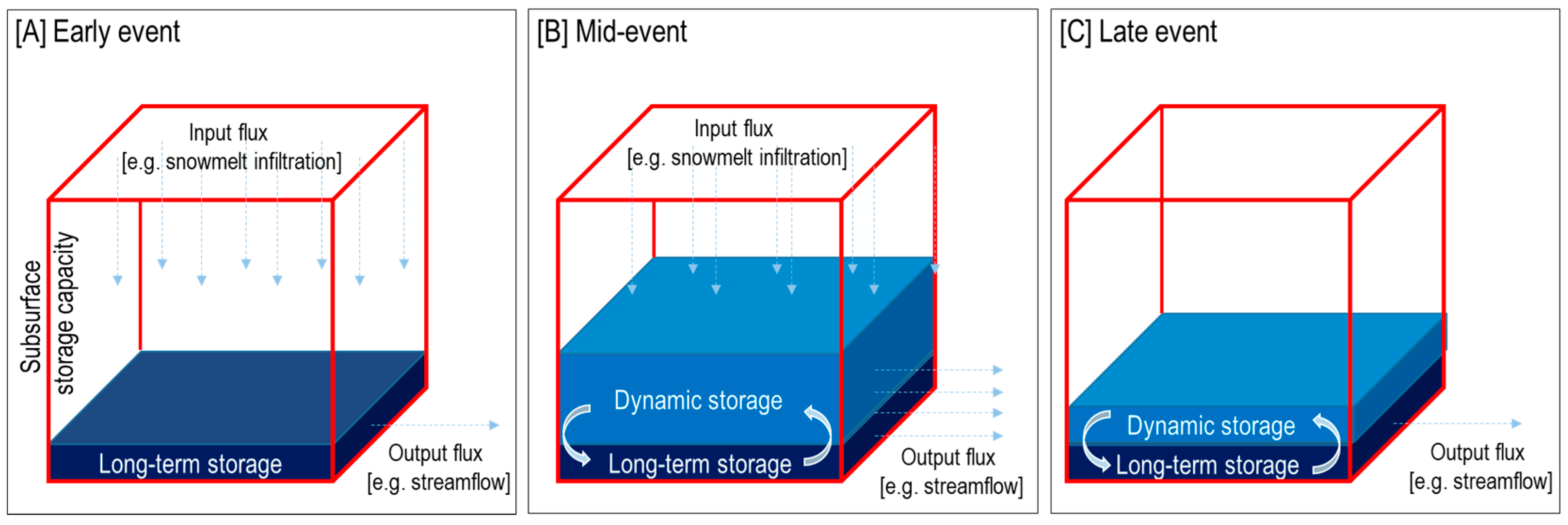
A conceptual model of these sub-event scale differences along a time series for a hydrologic event (
Figure 1) shows that as the hydrologic input event occurs, a given volume of water infiltrates into the subsurface, resulting in sub-event scale changes in mass-balance and dynamic storage. This example shows a snowmelt event for which the storage capacity of the catchment is not reached, and the long-term storage is consistent from year to year. Event-response ellipses quantify intra-event water balance differences using simple, scalable methods to measure the role of dynamic storage, which can then be compared across space and time.
The method to produce event-response ellipses is first presented in terms of an idealized system, then applied to two heavily instrumented study sites. The results from the study sites are then compared to the results from the idealized system. Departure from the idealized system results may show limitations of the event-response ellipse model, or full accounting of components of the water balance. We expect that if there are missing components of the water balance, such as long-term storage or glacial melt, the event-response ellipse will show more scatter or deviation from the idealized system. These instances do not mean that the event-response ellipse approach does not work, but rather, it provides insight regarding the closure of the water balance, identifying where data collection and validation may be required, or where processes are occurring on a substantially different time scale.
2.1. Event-Response Ellipses in an Idealized System
Parametric sinusoidal functions were chosen to represent the hydrologic event and response magnitude time series (
Figure 2 and
Figure 3). The seasonal periodicity of snowmelt (each cycle including a winter freeze up, snowpack accumulation, and melt) make snowmelt-dominated systems ideal as hydrologic events for testing this method; however, we believe that the concept could hold to more generalized time series water balance data in systems where sufficient intermediate timesteps and complete input and output flux values are available, though more experimentation is needed. In this idealized system, a parametric sinusoidal function was used to simulate a hydrologic event over time, then this original ‘event function’ was modified to create a ‘response function’ through phase shift (δ) and magnitude (α) variables to represent an idealized system output hydrograph.
In this idealized response system, the event function of hydrologic flux over time
f(
t) was represented as half of a period of a sine wave (Equation (2)). Response functions,
g(
t) and
h(
t), were then generated using incremental changes in function modifiers δ and α (Equations (3) and (4)).
Event-response ellipses are generated when the event function, f(t), is plotted against a response function after either a phase change, g(t) or a magnitude change, h(t).
2.1.1. Event-Response Ellipse Characteristics Relations
The modifiers of the response functions (phase shift and magnitude) are related to the resulting event-response ellipse characteristics of eccentricity and angle, respectively. The relations of these measurable ellipse characteristics to the difference between the event and response functions allow for the translation of values that are generated in this idealized system, to later be compared to the observed catchment data.
Phase shift, δ, is the amount by which the idealized response function is shifted in time (
t) relative to the event function (Equation (2),
Figure 3). The relative shift, σ, of the response function is calculated as a ratio of the phase shift to the flux period (π) (Equation (5)).
Eccentricity ranges from zero, a circle, to one, a straight line. The formula for eccentricity includes the semi-major axis length (
a) and semi-minor axis length (
b) (Equation (6)). There is a statistically significant, linear relation (r-squared = 0.99,
p-value < 0.00001) between relative phase shift (
) and the semi-minor axis length (
b) (Equation (7)). The formula for the calculation of eccentricity was adapted using the relationship in Equation (7) to directly relate eccentricity to phase shift (Equation (8)).
The area under an idealized system function,
A, is the cumulative flux over the time period. It is directly related to the amplitude (α), which is the measure of the maximum value of the simulated flux (
Figure 3). The area under
f(
t) is equal to the integral of the sine function from 0 to π, or 2. The area under
h(
t) is the amplitude multiplied by 2 (Equation (9)).
To describe the relation between area, amplitude, and angle, a relative change in magnitude between the event and response functions was calculated. This change in magnitude is described as the ratio of the area under the response function over the area under the event function. This measure relates back to the real system as the cumulative flux of the event and response, respectively. The ratio of area is directly related to the ratio of amplitude (Equation (10)):
The angle of the ellipse is measured between the x-axis to the semi-major axis of the event-response ellipse. The semi-major axis of an event-response ellipse that originates at the origin can be overlapped by a line drawn from the origin to the maximum value of the x- and y-axes. These maximum x- and y-axes values are then legs of a right triangle, and the ratio of these values can be used to calculate the angle of the semi-major axis through a trigonometric relation between the change in magnitude and conversion from radians to degrees (Equation (11)):
2.1.2. Event-Response Ellipses in an Idealized System
The influence of idealized response function modifiers to the shape of the resulting event-response ellipses were independently measured by plotting the initial function,
f(
t) (Equation (2)), versus
g(
t) (Equation (3)) and then versus
h(
t) (Equation (4)) to create Lissajous curves [
28], which were then used to calculate the ellipse characteristics, eccentricity, and angle, and develop relations between them and relative phase shift percent (δ) and change in magnitude (
) (
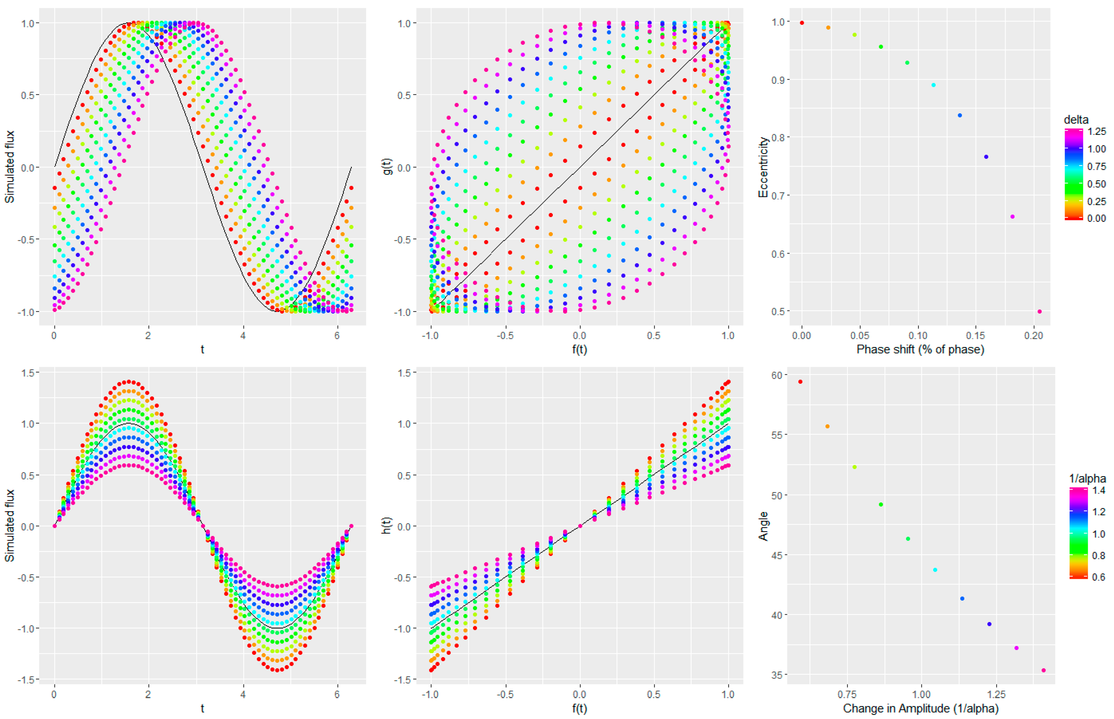
Figure 4).
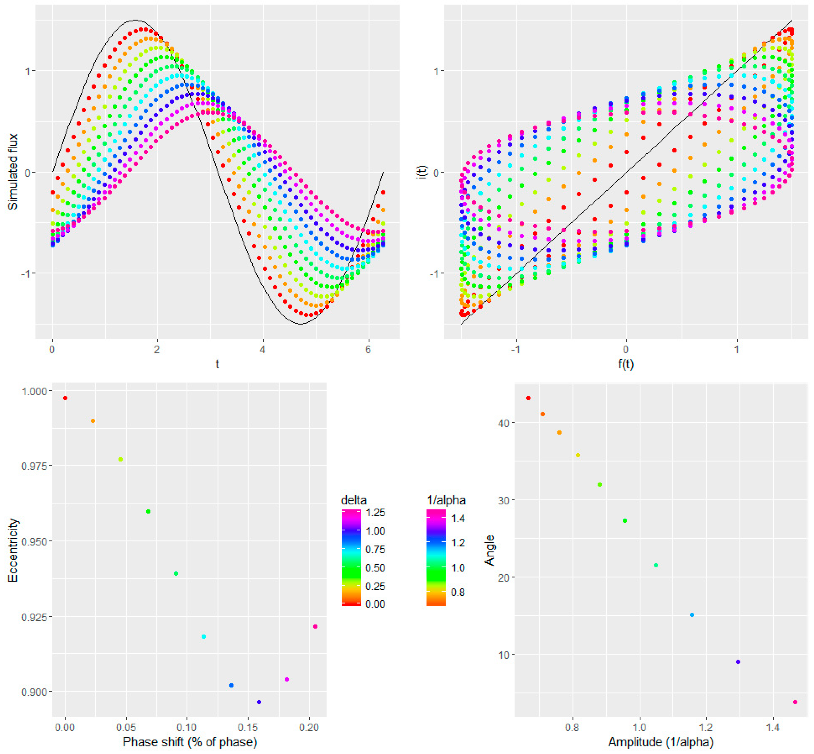
In
Figure 4, event and response functions (left), event-response ellipses (center), and relation to event-response ellipse characteristics (right) are shown using incremental changes to δ and
(color), change in δ (upper), change in α (lower) (
Figure 4). The black line shows the unmodified event function,
f(
t) (left), or when
f(
t) is equal to
g(
t) and
h(
t) (center). The relations between the event-response ellipse characteristics and the function modifiers’ eccentricity, δ (upper) and angle, α (lower) are each nonlinear.
2.2. Conceptual Model Translation from Idealized to Real Data
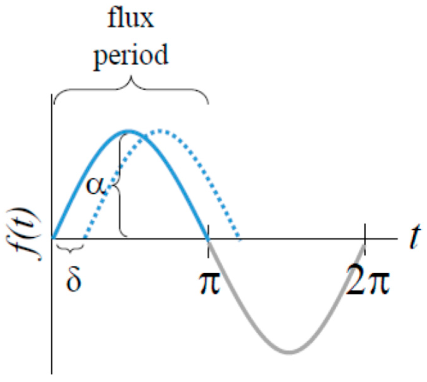
Relating these idealized system functions to real-world data requires a translation to a conceptual model of a hydrologic event and response in a catchment. The phase shift of the idealized functions can be thought of as the time lag of the hydrologic response relative to the hydrologic event, which could be caused by the physical routing of water through the catchment via overland or subsurface flowpaths. The change in magnitude between the idealized functions can be thought of as the change in the peak values of the event and response, due to the contribution or loss of stored water. Conceptually, the area under the event or response function is equal to the volume of water entering or leaving the catchment, respectively. A change in magnitude (amplitude) would therefore be related to a change in volume, or a non-zero catchment water balance; a decrease from snowmelt to discharge would mean a contribution to long-term storage, whereas an increase from event to response would mean a contribution from long-term subsurface storage to discharge. A zero magnitude difference results in an event-response ellipse angle of 45 degrees, and the greater the magnitude difference, the greater the difference of angle from 45 degrees (
Figure 3). An angle greater than 45 degrees has a response magnitude that is greater than the event magnitude, while an angle of less than 45 degrees has an event magnitude greater than the response magnitude.
The consistency of event-response ellipse metrics (eccentricity and angle) reflects the consistency of the catchment response, while conversely, if event-response ellipses are variable, the catchment response is also variable. The event-response ellipse synthesizes the catchment response by integrating and relating the event and response data over time. Event-response ellipse metrics are relative: when the event and response fluxes vary asynchronously, the event-response ellipse metrics are variable; but if event and response vary in concert, event-response ellipse metrics are consistent.
2.3. Event-Response Ellipse Assumptions, Limitations, and Potential Uses
This conceptual, idealized system was used to find the relations between changes in phase shift, and magnitudes between event and response functions. The application of this method to generate event-response ellipses with real data is expected to be limited to specific systems and conditions: this method is not expected to perform well (i.e., a poor fit to a modeled ellipse based on a qualitative visual assessment) in environments where all components of the water balance are not accounted for, where there is no infiltration to storage reservoirs with a residence time that is less than the event period, and where the timespan of the event and response is not long enough for adequate measurements to describe the system during the event and response. Examples include incongruent data-to-process temporal resolution (i.e., when there is not an adequate intermediate temporal resolution to describe the processes, or a system for which not all major components of the water balance are measured).
An application of the event-response ellipse method that results in a scattered fit (poor performance) provides insight to the hydrology of the system, because of the relation to a controlled, idealized system. The location and magnitude of the scatter in the event-response ellipse relative to the idealized system could be used to define where the data is, to describe the components of the water balance that are poorly understood or poorly measured. The increased scatter of annual applications relative to the averaged application of the event-response ellipse method also shows that while single-day flux values may vary more, averages over several events (snowmelt seasons) may provide a better understanding of the role of dynamic storage in the catchment, for comparison across catchments.
A scattered fit could show the dominance of an otherwise unaccounted-for contribution to streamflow, such as other precipitation events, glacial melt, or long-term storage. For example, where data show that a more than expected flux in or out could be an indication that during this time, within the event-response there is another process that has a more dominant than expected role in the hydrology of the system. Thus, an application with a result that shows scatter compared to the idealized system could still be quite useful as an indicator of where additional instrumentation and data collection to better characterize components of the water balance are needed. Alternatively, catchments that show a similar response to the idealized system (minimal scatter) are likely to have all components of the water balance accounted for, and dynamic storage as a dominant hydrologic process.
Real-world systems are also likely to be modified by both phase shift and magnitude within a given event period (Equation (12)):
The relation between the function modifiers (δ and α) and response ellipse characteristics (eccentricity and angle) are non-linear (
Figure 5).
3. Application to Study Area Catchments
Two study catchments were selected for this study because of their (a) snowmelt-dominated hydrology, which allows us to examine a single prolonged hydrologic event and response; and (b) existing robust and comprehensive data, including modelled daily snowmelt and measured daily streamflow; and (c) known difference in storage capacity. The following section further describes these catchments, the snowmelt model, previous studies of storage capacity, and application of the event-response ellipse method.
3.1. Study Area and Data Descriptions
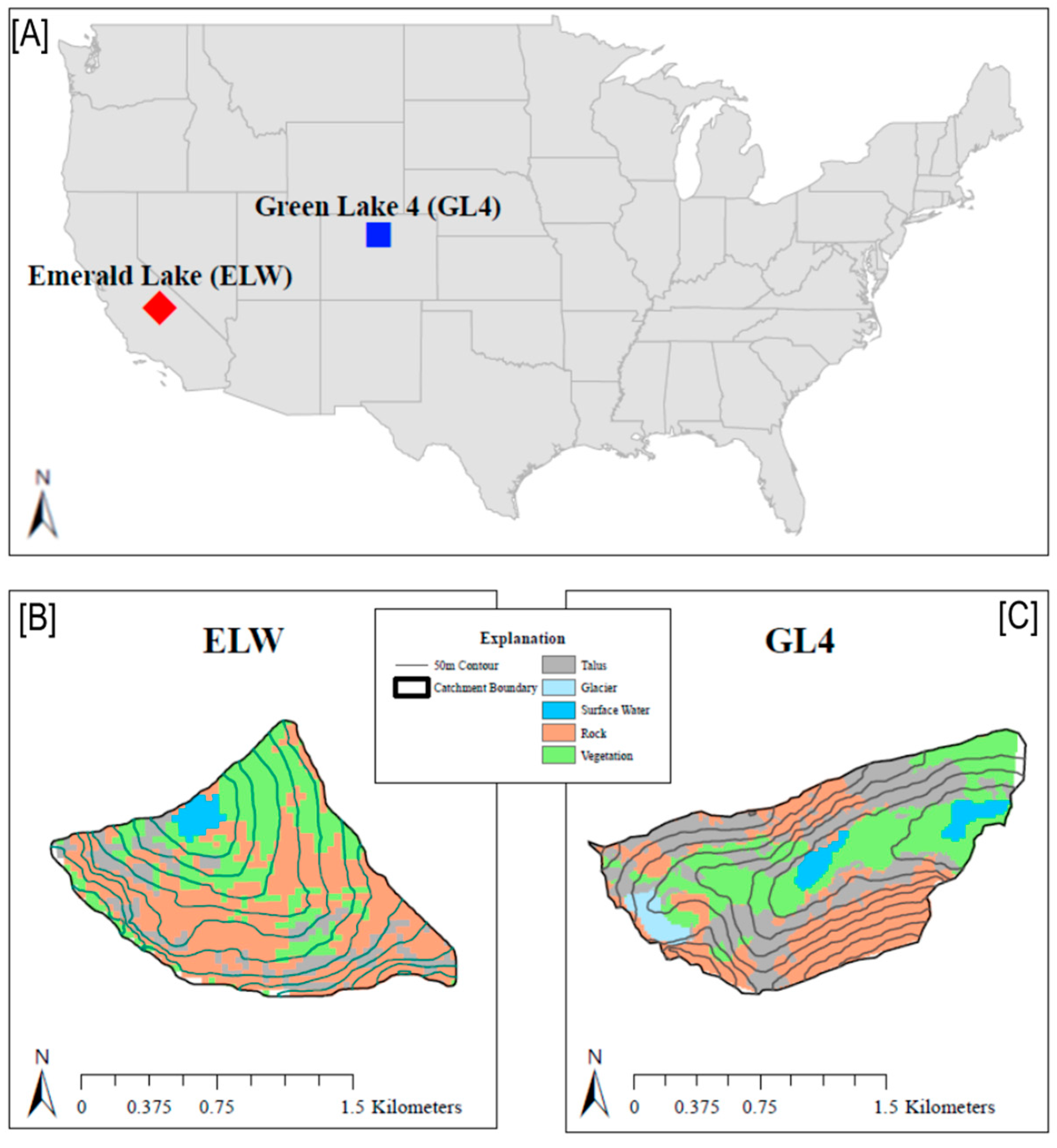
The two catchments selected for this study are located in alpine (above tree-line) headwaters. The Emerald Lake Watershed (ELW) is located in the Tokopah Valley within the Southern Sierra Nevada in California, USA, and Green Lake 4 (GL4) is located in the Green Lakes Valley within the eastern slope of the Front Range in Colorado, USA (
Figure 6). ELW is located at 36°35’ N, 118°40’ W, has an area of 1.20 km
2, and spans from 2800 m to 3416 m above sea level from Emerald Lake to Alta Peak, respectively. GL4 is located at 40°03’ N, 105°35’ W, has an area of 2.25 km
2, and spans from 3560 m to 4024 m above sea level from the GL4 outlet to Navajo Peak, respectively. Both catchments receive greater than 75% of the total annual precipitation as snow [
31,
32], which melts between April and August each year. ELW and GL4 catchments have been the subjects of a variety of catchment-scale studies, many of which have focused on hydrochemistry through tracer and hydrograph separation techniques [
32,
33,
34,
35,
36,
37]. Hydrologic residence time has been estimated in ELW to be on the order of hours to days [
33], and just over a year in GL4 [
37]. Previous studies have shown these two catchments have different storage capacities: GL4 has substantially greater storage capacity than ELW [
32,
34,
35,
38,
39,
40].
Energy balance snowmelt model results were used as the daily hydrologic event data for the application to the study areas. This study uses the modelled hourly, spatially-distributed (gridded) snowmelt output that pre-processes sublimation loss from the snowpack [
38] to provide hydrologic input data for analysis, and it thereby inherits the assumptions of this model. Those assumptions and errors include: possible overestimation of early season snowmelt (due to resetting snowpack cold content to zero each midnight), and exceeding of the timing of end-of-season snowmelt (due to cloud coverage and satellite over-pass schedule). These model overestimates may not be consistent between years or catchments; however, snowmelt model results provide the best available daily snowmelt flux values derived from the same methodology for both study catchments. The use of eleven years of snowmelt model data should help to minimize any overestimates for any given year from these sources of error.
Spatially distributed snowmelt model results [
38,
41] provide an important quantitative improvements over the extrapolation of point-measured precipitation [
42,
43]. Input data for the snowmelt models included geospatial and atmospheric measurements from in situ climate data stations to model hourly snowmelt for each 30 m grid cell within the model domains [
38,
41]. These snowmelt models have been shown to explain 61–84% of inter-annual variability of snow water equivalent (SWE) based on snow survey data. This energy balance snowmelt model accounts for the removal of water through sublimation processes (Equation (1)) during the snowmelt season in these catchments. The snowmelt output of these models provided a robust spatially distributed estimate of hydrologic event input for event-response ellipse calculations.
Spatiotemporal normalization of data was required to allow for comparison between years and catchments. Hourly modelled snowmelt volumes were aggregated to daily data, and the gridded output was clipped to the spatial boundary of the catchment area and aggregated to provide the daily snowmelt input to the catchment in meters. Measured daily streamflow volumes were normalized by catchment area to provide daily streamflow values.
3.2. Event-Response Ellipse Generation
Catchment-area normalized average daily snowmelt and streamflow were fit with an ellipse using the hysteresis package in R [
44]. These time-averaged event-response ellipses allowed for cross-site comparison. Event-response ellipses were also generated for each snowmelt season using the same method, which allowed for inter-annual comparisons.
The temporal scale for the application of event-response ellipses to real data was statically defined as day-of-year 60 to 243 (calendar dates 1 March to 31 August for non-leap years) for each year in the study period. This restriction follows the idealized system methodology of defining the period of the event and response functions. In the real world, streamflow may continue to flow past day-of-year 243; however, these data were not included in these calculations. Removing these data from the analysis may result in an incomplete response ellipse if the hydrologic processes (e.g., subsurface flowpaths) have a longer residence time than this restricted response period; however, the consistent time period allows for direct comparison of event-response ellipse metrics.
To compare real data with the expected response in an idealized system, the phase shift and magnitude change between snowmelt and streamflow were converted to relative terms. To calculate the phase shift of real data, first, the centroid of annual hydrologic fluxes (
Flux50) was calculated for each year of the study period (Equation (13)):
where
j is the Julian day of year, and
Flux50 was calculated for snowmelt (
Melt50) and streamflow (
Q50) fluxes. The
Flux50 values
Q50 and
Melt50 were then used to calculate the timing difference for each year of the study [
5] (Equation (14)):
The timing difference, in days, describes the lag between Melt50 and Q50 in each catchment for each year. The timing difference in days was transformed to a percentage of the total length of the snowmelt season (e.g., the phase) as a percentage, and was used as σ to relate these real data to the response in an idealized system. Daily hydrologic fluxes over each snowmelt season were used to calculate a change in area under the hydrograph time series ‘curve’, which is directly related to the change in magnitude, by dividing the catchment area-normalized annual streamflow by the catchment area-normalized annual snowmelt flux.
3.3. Study Area Results
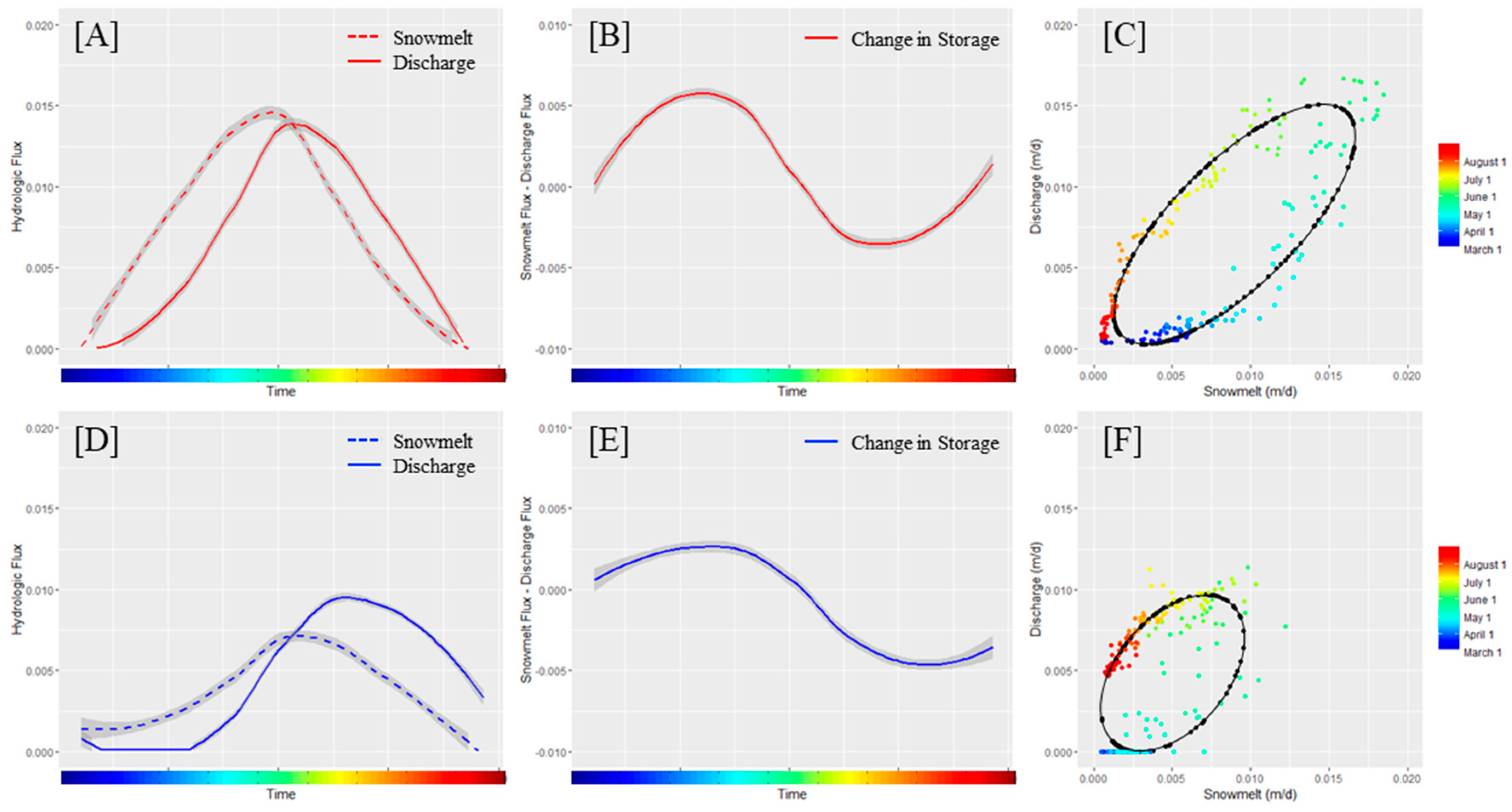
Eleven seasons (1996–2006) were evaluated for event-response ellipses in GL4 and ELW, providing a robust evaluation of the extent to which storage capacity plays a role in catchment response. The daily mean values over the study period were also used to create catchment-specific event-response ellipses to compare across sites (
Figure 7). Individual year event-response ellipse characteristics (e.g., eccentricity and angle) and summary statistics of these values are shown in
Table 1.
The results presented in
Figure 7 show average daily values for ELW and GL4 produce different, distinct event-response ellipses. The magnitudes of daily fluxes (snowmelt, discharge, and change in storage) are greater in GL4 than ELW. Both catchments have a counterclockwise event-response ellipse, which shows the evolution over the season from higher snowmelt at the beginning of the season, leading to higher discharge later in the season. The event-response ellipse characteristics (eccentricity and angle) are different for ELW and GL4. Event-response ellipse eccentricity values are: 0.92 at ELW and 0.79 at GL4. Event-response ellipse angle values are: 43.5 degrees at ELW and 49.3 degrees at GL4.
The results presented in
Table 1 show similar standard deviations (sd) of timing difference (12 days for ELW, 11 days for GL4), and higher sd of residual flux in ELW (0.28 m) relative to GL4 (0.13 m). The event-response ellipse characteristic values are different for the two study areas. The annual eccentricity is more consistent in ELW (sd: 0.04) relative to GL4 (sd: 0.14). The annual ellipse angle values are more consistent in ELW (sd: 12 degrees) relative to GL4 (sd: 54 degrees).
4. Discussion
This study presents the methodology and site-specific application of event-response ellipses. Event-response ellipses were generated for daily data averaged over 11 snowmelt seasons, from 1996 to 2006, for a storage-limited catchment (ELW) and a non-storage limited catchment (GL4). These daily averaged values produced two different event-response ellipses that were used to measure the difference in dynamic and long-term storage in these catchments.
Results show that the event-response ellipse eccentricity is greater (less round) in ELW (0.92) relative to GL4 (0.79). Using the relations developed in the idealized system (
Figure 4), this indicates a smaller phase shift (timing difference) between snowmelt and streamflow. The event-response ellipse angles are both near 45 degrees; 43.5 degrees in ELW and 49.3 degrees in GL4. If there was no difference in magnitude, this angle is expected to be 45 degrees. In ELW, the 1.5 degree difference is less than the 4.3 degree difference at GL4, showing that the change in magnitude between snowmelt and streamflow is larger in GL4. In addition, the angle is less than 45 degrees in ELW, and greater than 45 degrees in GL4. This indicates that the magnitude of streamflow is less than the magnitude of snowmelt in ELW, whereas the magnitude of streamflow is more than the magnitude of snowmelt in GL4. The increase in magnitude at GL4 is likely to be due to the contribution from other sources of stored water that were not considered in the snowmelt values for this study.
In addition to other sources of water from long-term storage in GL4, the fixed time period of analysis has also impacted results through truncating the output streamflow. The time period remained static for all data in part to facilitate comparison between years and catchments, but also because beyond this date precipitation as rainfall, which does not have an adequate spatially distributed dataset to add as an input. Further analysis where improved spatially distributed rainfall and snowmelt data have been collected will contribute to testing the event-response ellipse framework presented in this study. This may be an additional limitation of this method; the response period length needs to be within the time frame before the next input event occurs.
These event-response ellipse results add to the understanding that is gained from previous hydrochemical investigations: ELW is likely to be more vulnerable in shorter, quicker snowmelt seasons, due to limited subsurface hydrologic storage and the lack of contribution from other long-term storage reservoirs to mitigate snowmelt variability. Previous studies have used hydrochemical and isotopic analyses to measure the relative storage capacities of ELW and GL4 [
33,
45,
39]. The contribution in GL4 from permafrost and glacial melt, a surficial long-term storage reservoir, has been shown to play an important role in the hydrochemistry of the catchment [
45,
46]. The combination of these contributions from long-term storage with larger dynamic storage capacity could be the reason for why GL4 exhibits a disconnection between snowmelt and streamflow (greater distance from fit ellipse) in the annual event-response ellipses. These long-term reservoirs are not present in ELW, where event-response ellipses have more consistent characteristics. The reduced role of dynamic storage relative to long-term storage in GL4 increases the resiliency of hydrologic processes to changing snowmelt conditions, at least within the time frame of this study. There may be a limit to the resilience that long-term storage can provide to snowmelt variability, which has not yet been reached in these study catchments.
A broader application of event-response ellipses could be used to provide characterization and evaluation metrics for snowmelt-dominated hydrologic systems. Reduced snowpack and slower snowmelt [
3,
5,
47] under future climate scenarios [
48,
49] may reduce the water availability in the western United States [
49]. The role of subsurface storage as a physical buffer between the seasonal snowmelt and streamflow is critical to quantifying the extent that snowmelt-dominated water resources in the western United States will be impacted by climate change [
32,
4,
5]. Less variability in event-response ellipse values in ELW relative to GL4 show a limited role in mitigating earlier-onset snowmelt seasons where storage capacity is limited. Without contribution to the long-term storage or glacial melt (which are important in GL4), ELW relies more on dynamic storage to mitigate the impacts of climate change on the timing of streamflow at the catchment outlet. The quantification of these catchment-scale dynamic storage processes that mitigate the interannual variability of snowmelt could lead to the characterization of the vulnerability of headwater ecosystems to continued climate change. Without dynamic subsurface storage to mitigate the snowmelt variability, storage-limited aquatic ecosystems are more likely to be vulnerable to changes in snowmelt timing.
The event-response ellipse is a novel approach to the evaluation of our understanding of the volumetric and temporal components of the water balance. While applications in this study were limited to two highly instrumented snowmelt-dominated headwater catchments, this approach could be used to measure and compare the change in storage component, and the timing of water balance on a broad scale. The application of this method to assess the water balance using remotely-sensed or modelled water balance components could provide a framework for a comparison of the processes that are occurring at different spatial and temporal scales.
A departure from the idealized response system, resulting in a scattered fit to the expected event-response ellipse, is expected in an application of this method. This scatter can be indicative of (a) inadequate temporal resolution of data relative to the length of the event and response; (b) inadequate representation of the hydrologic input and output fluxes to the catchment; (c) or dynamic storage does not play a dominant role at the catchment and event scales. Results that show a scattered fit for applications of this method could also be used to identify areas where components of water balance are not adequately measured or represented in hydrologic models. For example, we know that at GL4, glacial melt exists, but it was not included in the input flux component. This allowed for a test of the response-ellipse method, which shows more scatter in every year of the GL4 ellipses than the application without glacial melt input (ELW).
5. Conclusions
The event-response ellipse method was introduced using idealized parametric functions to provide a mathematical framework before its application in two snowmelt-dominated study catchments. This approach to measuring the dynamic storage processes provides a quantitative evaluation of the water balance closure between the hydrologic event input and the catchment streamflow output within an event-response time frame. This method also allows for a comparison across space and time of the role of the dynamic storage of a catchment system through event-response ellipse characteristics, providing an ability to assess resilience to event variability. Areas where dynamic storage plays a large role in buffering the physical variability of snowmelt timing en route to streamflow, such as ELW, could be more resilient to snowmelt variability in future climate conditions. Areas where long-term storage contributes to the physical buffering capacity of the catchment, such as GL4, may be more vulnerable to change in timing of streamflow (and therefore water availability for ecosystems) if these long-term storage reservoirs are reliant on limited supply, such as melting glaciers or permafrost.
Author Contributions
J.M.D. conceived and directed the study, as well as wrote the paper. T.M., N.P.M., and T.P.A.F. further improved the concept and writing of the manuscript. N.P.M., M.W.W., and J.O.S. contributed data and model output for analysis. T.M., N.P.M., and J.M.D. secured funding.
Funding
U.S. Geological Survey National Water Census and National Science Foundation EAR 0738748.
Acknowledgments
GL4 streamflow data were collected and managed by Mark Williams through the Mountain Research Station of the University of Colorado at Boulder and Niwot Ridge Long-Term Ecological Research (LTER), with funding from the National Science Foundation (NSF). ELW streamflow data collection was managed and provided by James Sickman through the University of California, Riverside. The snowmelt model output data used in this analysis were provided by Steven Jepsen. These daily data are included as supplemental information. This research was a part of the NSF grant EAR0738748. Any use of trade, firm, or product names is for descriptive purposes only and does not imply endorsement by the U.S. Government.
Conflicts of Interest
The authors declare no conflicts of interest.
References
- Barnett, T.P.; Adam, J.C.; Lettenmaier, D.P. Potential impacts of a warming climate on water availability in snow-dominated regions. Nature 2005, 438, 303–309. [Google Scholar] [CrossRef] [PubMed]
- Carroll, S.S.; Cressie, N. Spatial modeling of snow water equivalent using covariances estimated from spatial and geomorphic attributes. J. Hydrol. 1997, 190, 42–59. [Google Scholar] [CrossRef]
- Mote, P.W.; Hamlet, A.F.; Clark, M.P.; Lettenmaier, D.P. Declining mountain snowpack in western North America. Bull. Am. Meteorol. Soc. 2005, 86, 39–50. [Google Scholar] [CrossRef]
- Christensen, N.S.; Wood, A.W.; Voisin, N.; Lettenmaier, D.P.; Palmer, R.N. The Effects of Climate Change on the Hydrology and Water Resources of the Colorado River Basin. Clim. Chang. 2004, 62, 337–363. [Google Scholar] [CrossRef] [Green Version]
- Clow, D.W. Changes in the Timing of Snowmelt and Streamflow in Colorado: A Response to Recent Warming. J. Clim. 2010, 23, 2293–2306. [Google Scholar] [CrossRef]
- Barnhart, T.B.; Molotch, N.P.; Livneh, B.; Harpold, A.A.; Knowles, J.F.; Schneider, D. Snowmelt rate dictates streamflow. Geophys. Res. Lett. 2016. [Google Scholar] [CrossRef]
- Soulsby, C.; Piegat, K.; Seibert, J.; Tetzlaff, D. Catchment-scale estimates of flow path partitioning and water storage based on transit time and runoff modelling. Hydrol. Process. 2011, 25, 3960–3976. [Google Scholar] [CrossRef]
- Kendall, K.A.; Shanley, J.B.; McDonnell, J.J. A hydrometric and geochemical approach to test the transmissivity feedback hypothesis during snowmelt. J. Hydrol. 1999, 219, 188–205. [Google Scholar] [CrossRef]
- Adam, J.C.; Hamlet, A.F.; Lettenmaier, D.P. Implications of global climate change for snowmelt hydrology in the twenty-first century. Hydrol. Process. 2009, 23, 962–972. [Google Scholar] [CrossRef]
- Ajami, N.K.; Hornberger, G.M.; Sunding, D.L. Sustainable water resource management under hydrological uncertainty. Water Resour. Res. 2008, 44, W11406. [Google Scholar] [CrossRef]
- Frei, A.; Armstrong, R.L.; Clark, M.P.; Serreze, M.C. Catskill Mountain Water Resources: Vulnerability, Hydroclimatology, and Climate-Change Sensitivity. Ann. Assoc. Am. Geogr. 2002, 92, 203–224. [Google Scholar] [CrossRef]
- Matonse, A.H.; Pierson, D.C.; Frei, A.; Zion, M.S.; Anandhi, A.; Schneiderman, E.; Wright, B. Investigating the impact of climate change on New York City’s primary water supply. Clim. Chang. 2012, 116, 437–456. [Google Scholar] [CrossRef]
- Williams, M.W.; Seibold, C.; Chowanski, K. Storage and release of solutes from a subalpine seasonal snowpack: Soil and stream water response, Niwot Ridge, Colorado. Biogeochemistry 2009, 95, 77–94. [Google Scholar] [CrossRef]
- Ajami, H.; Troch, P.A.; Maddock, T.; Meixner, T.; Eastoe, C. Quantifying mountain block recharge by means of catchment-scale storage-discharge relationships. Water Resour. Res. 2011, 47, W04504. [Google Scholar] [CrossRef]
- Heidbüchel, I.; Troch, P.A.; Lyon, S.W.; Weiler, M. The master transit time distribution of variable flow systems. Water Resour. Res. 2012, 48, W06520. [Google Scholar] [CrossRef]
- Andermann, C.; Longuevergne, L.; Bonnet, S.; Crave, A.; Davy, P.; Gloaguen, R. Impact of transient groundwater storage on the discharge of Himalayan rivers. Nat. Geosci. 2012. [Google Scholar] [CrossRef]
- McGuire, K.J.; McDonnell, J.J. Hydrological connectivity of hillslopes and streams: Characteristic time scales and nonlinearities. Water Resour. Res. 2010, 46, W10543. [Google Scholar] [CrossRef]
- Penna, D.; Tromp-van Meerveld, H.J.; Gobbi, A.; Borga, M.; Dalla Fontana, G. The influence of soil moisture on threshold runoff generation processes in an alpine headwater catchment. Hydrol. Earth Syst. Sci. 2011, 15, 689–702. [Google Scholar] [CrossRef] [Green Version]
- Sproles, E.A.; Leibowitz, S.G.; Reager, J.T.; Al, E. GRACE storage-streamflow hystereses reveal the dynamics of regional watersheds. Hydrol. Earth Syst. Sci. Discuss. 2014, 11, 12027–12062. [Google Scholar] [CrossRef]
- McGuire, K.J.; McDonnell, J.J. A review and evaluation of catchment transit time modeling. J. Hydrol. 2006, 330, 543–563. [Google Scholar] [CrossRef]
- Bishop, K.; Seibert, J.; Köhler, S.; Laudon, H. Resolving the Double Paradox of rapidly mobilized old water with highly variable responses in runoff chemistry. Hydrol. Process. 2004, 18, 185–189. [Google Scholar] [CrossRef]
- Frisbee, M.D.; Phillips, F.M.; Weissmann, G.S.; Brooks, P.D.; Wilson, J.L.; Campbell, A.R.; Liu, F. Unraveling the mysteries of the large watershed black box: Implications for the streamflow response to climate and landscape perturbations. Geophys. Res. Lett. 2012, 39. [Google Scholar] [CrossRef] [Green Version]
- Birkel, C.; Soulsby, C.; Tetzlaff, D. Modelling catchment-scale water storage dynamics: Reconciling dynamic storage with tracer-inferred passive storage. Hydrol. Process. 2011, 25, 3924–3936. [Google Scholar] [CrossRef]
- Tetzlaff, D.; McNamara, J.P.; Carey, S.K. Measurements and modelling of storage dynamics across scales. Hydrol. Process. 2011, 25, 3831–3835. [Google Scholar] [CrossRef]
- Christophersen, N.; Hooper, R.P. Multivariate analysis of stream water chemical data: The use of principal components analysis for the end-member mixing problem. Water Resour. Res. 1992, 28, 99–107. [Google Scholar] [CrossRef]
- Weiler, M.; McGlynn, B.L.; McGuire, K.J.; McDonnell, J.J. How does rainfall become runoff? A combined tracer and runoff transfer function approach. Water Resour. Res. 2003, 39. [Google Scholar] [CrossRef] [Green Version]
- Huth, A.K.; Leydecker, A.; Sickman, J.O.; Bales, R.C. A two-component hydrograph separation for three high-elevation catchments in the Sierra Nevada, California. Hydrol. Process. 2004, 18, 1721–1733. [Google Scholar] [CrossRef]
- Lissajous, J. Memoire sur l’etude optique des mouvements vibratoires. Ann. Chim. Phys. 1849, 3, 140–231. [Google Scholar]
- Skøien, J.O.; Blöschl, G.; Western, A.W. Characteristic space scales and timescales in hydrology. Water Resour. Res. 2003, 39. [Google Scholar] [CrossRef] [Green Version]
- Blöschl, G.; Sivapalan, M. Scale issues in hydrological modelling: A review. Hydrol. Process. 1995, 9, 251–290. [Google Scholar] [CrossRef]
- Sickman, J.O.; Leydecker, A.; Melack, J.M. Nitrogen mass balances and abiotic controls on N retention and yield in high-elevation catchments of the Sierra Nevada, California, United States. Water Resources Research 2001, 37, 1445–1461. [Google Scholar] [CrossRef] [Green Version]
- Williams, M.W.; Losleben, M.; Caine, N.; Greenland, D. Changes in Climate and Hydrochemical Responses in a High-Elevation Catchment in the Rocky Mountains, USA. Limnol. Oceanogr. 1996, 41, 939–946. [Google Scholar] [CrossRef]
- Williams, M.W.; Brown, A.D.; Melack, J.M. Geochemical and Hydrologic Controls on the Composition of Surface Water in a High-Elevation Basin, Sierra Nevada, California. Limnol. Oceanogr. 1993, 38, 775–797. [Google Scholar] [CrossRef]
- Wolford, R.A.; Bales, R.C.; Sorooshian, S. Development of a Hydrochemical Model for Seasonally Snow-Covered Alpine Watersheds: Application to Emerald Lake Watershed, Sierra Nevada, California. Water Resour. Res. 1996, 32, 1061–1074. [Google Scholar] [CrossRef]
- Meixner, T.; Bales, R.C.; Williams, M.W.; Campbell, D.H.; Baron, J.S. Stream chemistry modeling of two watersheds in the Front Range, Colorado. Water Resour. Res. 2000, 36, 77–87. [Google Scholar] [CrossRef] [Green Version]
- Liu, F.J.; Williams, M.W.; Caine, N. Source waters and flow paths in an alpine catchment, Colorado Front Range, United States. Water Resour. Res. 2004, 40. [Google Scholar] [CrossRef] [Green Version]
- Cowie, R.; Williams, M.W.; Caine, N.; Michel, R. Estimated residence time of two snowmelt dominated catchments, Boulder Creek Watershed, Colorado. In Proceedings of the 78th Annual Meeting, Western Snow Conference, Logan, UT, USA, 19–22 April 2010. [Google Scholar]
- Jepsen, S.M.; Molotch, N.P.; Williams, M.W.; Rittger, K.E.; Sickman, J.O. Interannual variability of snowmelt in the Sierra Nevada and Rocky Mountains, United States: Examples from two alpine watersheds. Water Resour. Res. 2012, 48. [Google Scholar] [CrossRef] [Green Version]
- Perrott, D.; Molotch, N.P.; Williams, M.W.; Jepsen, S.M.; Sickman, J.O. Relationships between stream nitrate concentration and spatially distributed snowmelt in high-elevation catchments of the western United States. Water Resour. Res. 2014, 50, 8694–8713. [Google Scholar] [CrossRef]
- Tonnessen, K.A. The Emerald Lake Watershed Study: Introduction and site description. Water Resour. Res. 1991, 27, 1537–1539. [Google Scholar] [CrossRef]
- Molotch, N.P.; Meixner, T.; Williams, M.W. Estimating stream chemistry during the snowmelt pulse using a spatially distributed, coupled snowmelt and hydrochemical modeling approach. Water Resour. Res. 2008, 44, W11429. [Google Scholar] [CrossRef]
- Beven, K.J.; Hornberger, G.M. Assessing the Effect of Spatial Pattern of Precipitation in Modeling Stream Flow Hydrographs. J. Am. Water Resour. Assoc. 1982, 18, 823–829. [Google Scholar] [CrossRef]
- Tetzlaff, D.; Uhlenbrook, S. Significance of spatial variability in precipitation for process-oriented modelling: Results from two nested catchments using radar and ground station data. Hydrol. Earth Syst. Sci. Discuss. 2005, 9, 29–41. [Google Scholar] [CrossRef]
- Maynes, S.; Yang, F.; Parkhurst, A. hysteresis: Tools for Modeling Rate-Dependent Hysteretic Processes and Ellipses. 2015. Available online: https://cran.r-project.org/web/packages/hysteresis/index.html (accessed on 11 December 2018).
- Williams, M.W.; Knauf, M.; Caine, N.; Liu, F.; Verplanck, P.L. Geochemistry and source waters of rock glacier outflow, Colorado Front Range. Permafr. Periglac. Process. 2006, 17, 13–33. [Google Scholar] [CrossRef] [Green Version]
- Barnes, R.T.; Williams, M.W.; Parman, J.N.; Hill, K.; Caine, N. Thawing glacial and permafrost features contribute to nitrogen export from Green Lakes Valley, Colorado Front Range, USA. Biogeochemistry 2014, 117, 413–430. [Google Scholar] [CrossRef]
- Musselman, K.N.; Clark, M.P.; Liu, C.; Ikeda, K.; Rasmussen, R. Slower snowmelt in a warmer world. Nat. Clim. Chang. 2017, 7, 214–219. [Google Scholar] [CrossRef]
- Solomon, S.; Qin, D.; Manning, M.; Marquis, M.; Averyt, K.; Tignor, M.M.B.; Miller, H.L., Jr.; Chen, Z. Climate Change 2007—The Physical Science Basis: Working Group I; Cambridge University Press: Cambridge, UK, 2007; p. 996. [Google Scholar]
- Dettinger, M.; Udall, B.; Georgakakos, A. Western water and climate change. Ecol. Appl. 2015, 25, 2069–2093. [Google Scholar] [CrossRef] [PubMed]
Figure 1.
Conceptual model from the frame of reference of the subsurface storage capacity over the course of the hydrological event in three stages. (A) Early event shows a maximum snowpack beginning to infiltrate into the subsurface to add to the existing pre-event (long-term storage) water; (B) Mid-event shows snowpack continuing to infiltrate to contribute to the mix of dynamic and long-term storage waters; (C) Late event shows the depletion of the aggregation of mixed dynamic and stored waters after the end of snowmelt.
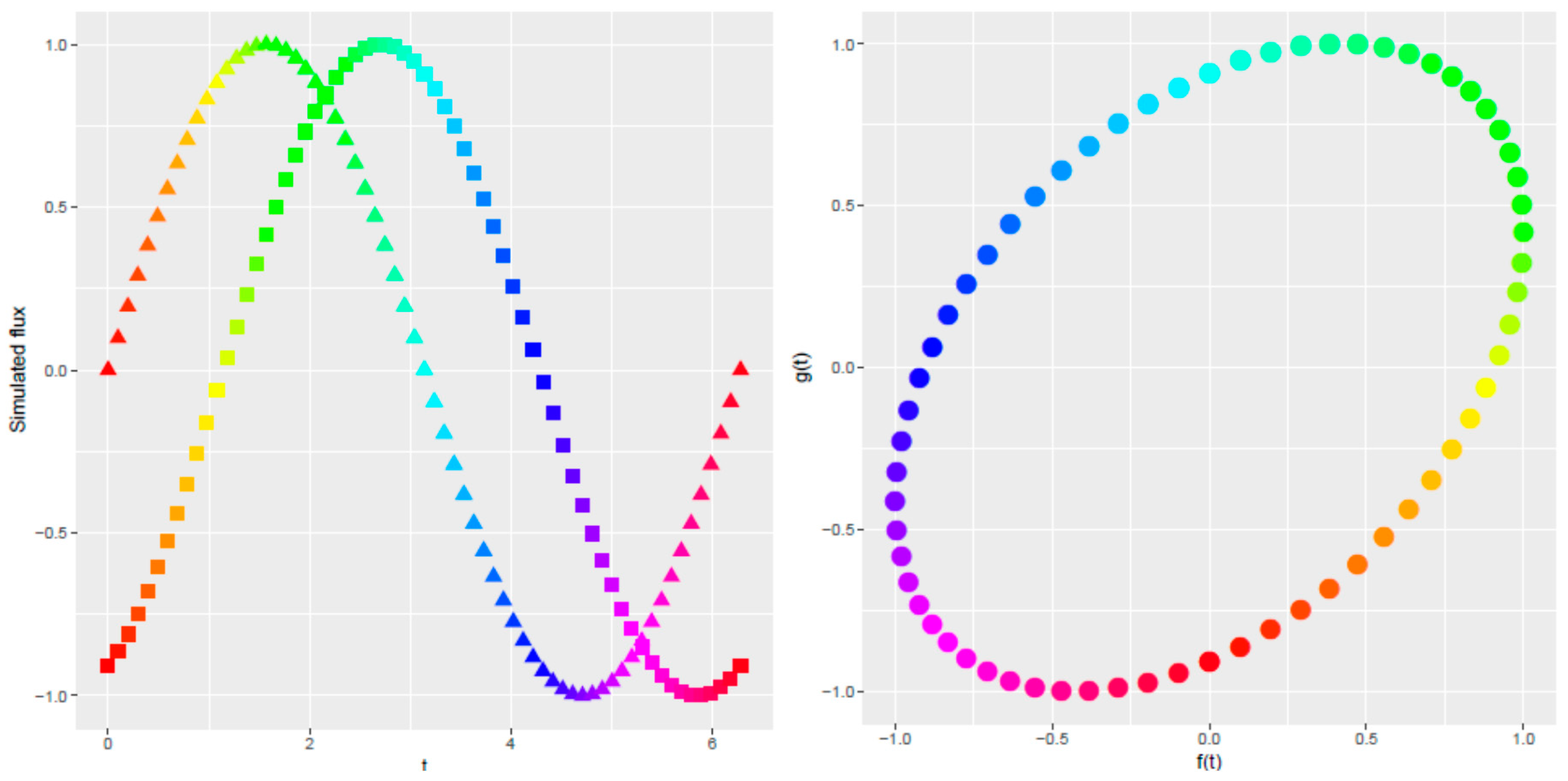
Figure 2.
Idealized catchment flux system (left, input shown with triangles, output shown with squares) over time (color), and corresponding idealized response ellipse (right).
Figure 2.
Idealized catchment flux system (left, input shown with triangles, output shown with squares) over time (color), and corresponding idealized response ellipse (right).
Figure 3.
A sine wave, f(t) = sin(t), 0 ≤ t ≤ 2t, was used to represent the hydrologic flux over time. Conceptually only half of a full period, 0 to t (solid line) was used to represent the snowmelt season, and the discharge was then described relative to the snowmelt season.
Figure 3.
A sine wave, f(t) = sin(t), 0 ≤ t ≤ 2t, was used to represent the hydrologic flux over time. Conceptually only half of a full period, 0 to t (solid line) was used to represent the snowmelt season, and the discharge was then described relative to the snowmelt season.
Figure 4.
Idealized system parametric functions and incremental changes in modified response functions are shown for phase shift (upper) and magnitude (lower). Left: The input function is shown in black, with incremental changes in the response functions shown in colors. Center: The original, unmodified function is plotted against the modified response function. Right: The phase shift is related to eccentricity, and magnitude is related to angle.
Figure 5.
Idealized system response when both phase shift and magnitude modifiers are applied. Upper: parametric functions and incremental changes in modified response functions are shown left, and event-response ellipses are shown right. Lower: relations of eccentricity to phase shift are shown left and angle to amplitude are shown right.
Figure 6.
General location in the Conterminous United States (A) and land coverage of the two study catchments: Emerald Lake Watershed (ELW), a 1.2 km2 catchment in the Sierra Nevada of California (B) and Green Lake 4 (GL4), a 2.25 km2 catchment in the Rocky Mountains of Colorado (C).
Figure 6.
General location in the Conterminous United States (A) and land coverage of the two study catchments: Emerald Lake Watershed (ELW), a 1.2 km2 catchment in the Sierra Nevada of California (B) and Green Lake 4 (GL4), a 2.25 km2 catchment in the Rocky Mountains of Colorado (C).
Figure 7.
Study catchment data using average daily data for the study period for ELW (A–C) and GL4 (D–F). Plots A and D show the smoothed time series of the mean daily snowmelt and the mean daily discharge flux data with a 95% confidence interval shown in dark grey. Plots B and E show the mean daily snowmelt flux minus the mean daily discharge flux, or the change in storage over time. Plots C and F show mean daily snowmelt versus mean daily discharge over time, and the fitted event-response ellipse.
Table 1.
Individual snowmelt event and response values for Emerald Lake Watershed (upper) and Green Lake 4 (lower), including event-response ellipse metrics of angle and eccentricity.
Table 1.
Individual snowmelt event and response values for Emerald Lake Watershed (upper) and Green Lake 4 (lower), including event-response ellipse metrics of angle and eccentricity.
| Emerald Lake Watershed |
|---|
| Year | Melt50 (DOY) | Q50 (DOY) | Cumulative Melt (m) | Cumulative Discharge (m) | Timing Difference (days) | Residual Flux (m) | Amplitude Change * | Phase Shift | Angle | Eccentricity * |
|---|
| 1996 | 140 | 149 | 1.08 | −1.32 | 9 | −0.24 | 1.67 | 9% | 52.91 | 0.86 |
| 1997 | 135 | 141 | 1.24 | −1.31 | 6 | −0.07 | 1.06 | 9% | 54.13 | 0.86 |
| 1998 | 166 | 167 | 1.43 | −1.79 | 1 | −0.35 | 0.92 | 3% | 48.70 | 0.90 |
| 1999 | 135 | 149 | 0.87 | −0.85 | 14 | 0.02 | 2.06 | 7% | 38.83 | 0.84 |
| 2000 | 142 | 147 | 1.03 | −0.89 | 5 | 0.14 | 0.82 | 3% | 46.68 | 0.90 |
| 2001 | 134 | 148 | 0.74 | −0.67 | 14 | 0.08 | 1.20 | 3% | 39.98 | 0.90 |
| 2002 | 130 | 151 | 1.26 | −0.77 | 21 | 0.50 | 0.53 | 14% | 27.04 | 0.82 |
| 2003 | 146 | 168 | 0.91 | −0.69 | 22 | 0.22 | 0.84 | 5% | 43.93 | 0.94 |
| 2004 | 115 | 155 | 1.24 | −0.61 | 40 | 0.63 | 0.56 | 15% | 14.69 | 0.81 |
| 2005 | 150 | 153 | 1.72 | −1.56 | 3 | 0.17 | 0.35 | 9% | 37.98 | 0.86 |
| 2006 | 149 | 148 | 1.79 | −1.62 | −1 | 0.17 | 0.87 | 8% | 44.88 | 0.90 |
| Green Lake 4 |
| Year | Melt50 (DOY) | Q50 (DOY) | Cumulative Melt (m) | Cumulative Discharge (m) | Timing Difference (days) | Residual Flux (m) | Amplitude Change * | Phase Shift | Angle (degrees) | Eccentricity * |
| 1996 | 155 | 199 | 0.64 | −0.80 | 44 | −0.16 | 1.24 | 17% | 1.11 | 0.77 |
| 1997 | 158 | 203 | 0.97 | −0.87 | 45 | 0.10 | 0.90 | 18% | 19.77 | 0.95 |
| 1998 | 153 | 198 | 0.72 | −0.81 | 45 | −0.08 | 1.12 | 9% | 35.73 | 0.77 |
| 1999 | 170 | 195 | 0.55 | −0.84 | 25 | −0.29 | 1.53 | 10% | 25.28 | 0.77 |
| 2000 | 153 | 194 | 0.58 | −0.71 | 41 | −0.13 | 1.23 | 17% | 0.22 | 0.92 |
| 2001 | 152 | 195 | 0.45 | −0.76 | 43 | −0.32 | 1.71 | 19% | 1.71 | 0.63 |
| 2002 | 139 | 199 | 0.33 | −0.53 | 60 | −0.21 | 1.63 | 31% | 36.63 | 0.81 |
| 2003 | 148 | 192 | 0.63 | −0.90 | 44 | −0.27 | 1.42 | 21% | 36.58 | 0.87 |
| 2004 | 128 | 197 | 0.52 | −0.69 | 69 | −0.17 | 1.32 | 36% | 151.84 | 0.54 |
| 2005 | 143 | 192 | 0.94 | −0.90 | 49 | 0.04 | 0.96 | 21% | 12.90 | 0.88 |
| 2006 | 145 | 190 | 0.53 | −0.76 | 45 | −0.24 | 1.45 | 22% | 142.54 | 0.58 |
© 2018 by the authors. Licensee MDPI, Basel, Switzerland. This article is an open access article distributed under the terms and conditions of the Creative Commons Attribution (CC BY) license (http://creativecommons.org/licenses/by/4.0/).

 ,
, 


