The Four Patterns of the East Branch of the Kuroshio Bifurcation in the Luzon Strait

Abstract

Based on the self-organizing map (SOM) method, a suite of satellite measurement data, and Hybrid Coordinate Ocean Model (HYCOM) reanalysis data, the east branch of the Kuroshio bifurcation is found to have four coherent patterns associated with mesoscale eddies in the Pacific Ocean: anomalous southward, anomalous eastward, anomalous northward, and anomalous westward. The robust clockwise cycle of the four patterns causes significant intraseasonal variation of 62.2 days for the east branch. Furthermore, the study shows that the four patterns of the east branch of the Kuroshio bifurcation can influence the horizontal and vertical distribution of local sea temperature.

1. Introduction

The Kuroshio, which is the strongest western boundary current in the Northwest Pacific (NWP), originates from the North Equatorial Current (NEC). Encountering Luzon Island, the NEC bifurcates into the northward Kuroshio Current and the southward Mindanao Current. Then the Kuroshio passes to the east of the Luzon Strait (LS), flows northward along the Taiwan Island into the East China Sea, and returns to the Pacific Ocean through the Tokara Strait. Because the Kuroshio transports a lot of heat and matter from low latitudes to mid-latitudes, it plays an important role in regional and global climate, and the marine ecosystem [1,2,3,4,5]. Meanwhile, the Kuroshio carries enormous amounts of momentum and kinetic energy, so it strongly interacts with mesoscale eddies and influences regional circulation such as the one in the LS [6,7,8,9,10,11].

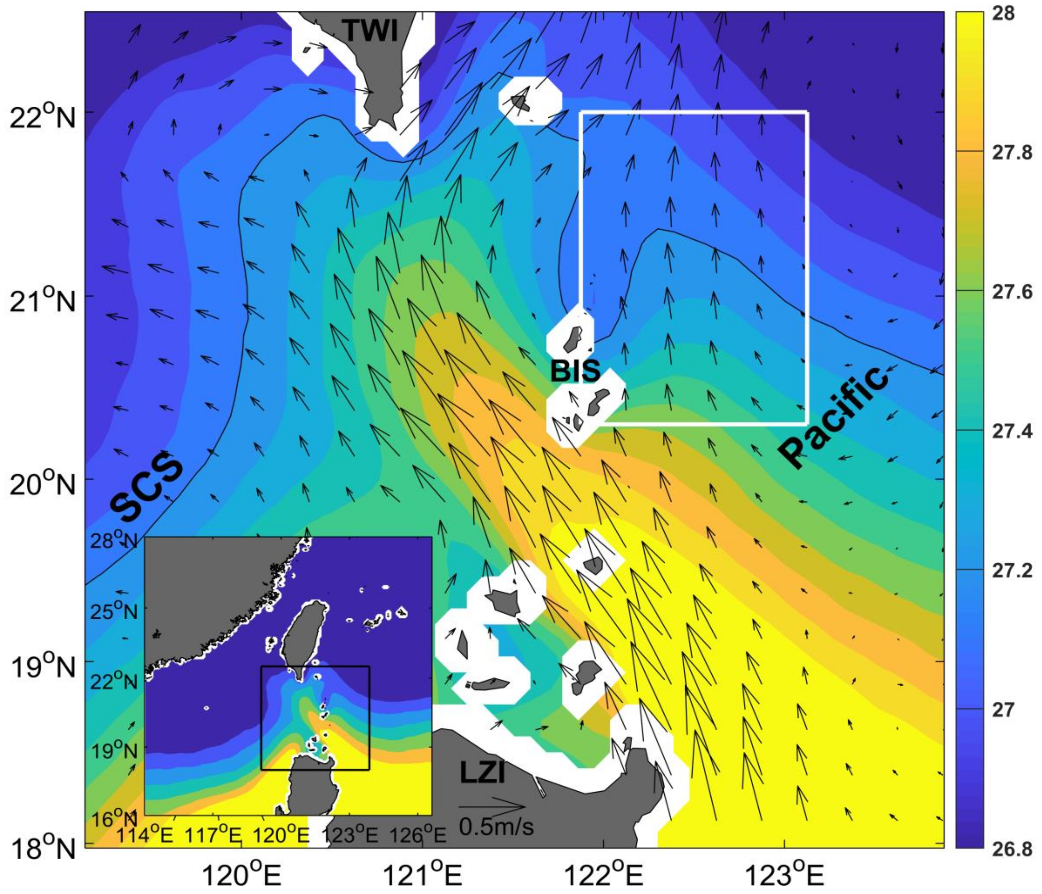
The LS, located between Taiwan Island and Luzon Island, is an important gap in the NWP (as shown in Figure 1). Affected by the Kuroshio, monsoon, mesoscale eddies, and topography, the circulation in the LS is very complicated, and has been studied extensively in previous literatures [8,9,12]. These studies have specifically discussed the interaction between the Kuroshio and mesoscale eddies: (1) the Kuroshio can generate mesoscale eddies by its own variation [11,13]; (2) the Kuroshio can affect mesoscale eddies in the NWP into the South China Sea [7,9]; (3) mesoscale eddies can alter the Kuroshio current field [8,10,14]; (4) interaction between the Kuroshio and mesoscale eddies can influence the local marine environment [14,15]. Although there are many related studies, some questions involving small and moderate ocean phenomena in the LS remain unclear.

The accumulation of high-resolution satellite remote sensing data enables us to better study small and moderate ocean phenomena. Based on high-resolution satellite remote sensing data and hydrological data along with numerical model simulations, the Kuroshio bifurcation phenomena in the LS has been put forward: The Kuroshio in the LS bifurcates into two branches located on the western and eastern sides of the Batanes Islands, and produces two warm tongues east of the LS [14]. The western branch is the main part of the Kuroshio, and its temporal and spatial variability has been widely studied [16,17,18,19]. However, the temporal and spatial variability of the eastern branch has hardly been studied and remains unclear, although its intensity is related to mesoscale eddies in the NWP [14]. The Kuroshio transports warm water from low latitudes to middle latitudes, so it can cause temporal and spatial variability of local sea temperature in most cases [14,16]. The east branch of the Kuroshio bifurcation, as a part of the Kuroshio, can produce a warm tongue [1] (Figure 1). However, it is unclear whether and how local sea temperature patterns are related to the patterns of the east branch. The purpose of the present study is to assess the variability of the east branch of the Kuroshio bifurcation and its effect on the local sea temperature. The rest of the paper is organized as follows: Section 2 briefly introduces the data and methods. Section 3 shows the temporal and spatial variability of the four patterns of the east branch and their effect on local sea temperature. Section 4 is a summary of this paper.

2. Data and Method

2.1. Data

Absolute dynamic topography (ADT) data and geostrophic current anomalies data were processed by Ssalto multimission ground segment (SSALTO)/Data unification and Altimeter combination system (DUACS) (AVISO, Ramonville Saint-Agne, France) and distributed by Archiving Validation and Interpretation of Satellite Data in Oceanography (AVISO) with support from CNES (Centre National d’Etudes Spatiales). The product is merged from Jason-1/2, Topex/Poseidon, Envisat, Geosat, and other altimeter missions. The raw satellite measurements have applied atmospheric corrections and a sea‒land transition. The product is computed on a Cartesian 1/4° × 1/4° spatial resolution and provides daily data from 1 January 1993 to the present [20,21].

Sea surface temperature (SST) is provided by Remote Sensing Systems (RSS, Santa Rosa, CA, USA). The product combines the through-cloud capabilities of the microwave SST data with the high spatial resolution and near-coastal capability of the infrared SST data. The microwave SST data is merged from Advanced Microwave Scanning Radiometer for Earth Observing System, WindSat, Tropical Rainfall Measuring Mission Microwave Images and Giant magnetoimpedance. The infrared SST data is merged from Moderate Resolution Imaging Spectroradiometer and Visible Infrared Imaging Radiometer Suite. The product has applied atmospheric corrections. It provides daily data from 1 July 2002 to present and its spatial resolution is 9 km × 9 km.

Hybrid Coordinate Ocean Model (HYCOM) reanalysis data is provided by HYCOM organization, which provides access to near-real-time global data-based ocean prediction system output. The HYCOM organization provides four HYCOM data-assimilation product, and we choose the product with the longest time span, which is from 2 October 1992 to 31 December 2012. The product has uniform 0.08 degree latitude/longitude grid between 80.48 °S and 80.48 °N and is interpolated to 40 standard z-levels. It provides sea surface height (SSH), temperature, salinity, meridional flow, and zonal flow.

2.2. Method

SOM can be classified as a type of clustering technique [22], and is an effective method for feature extraction and pattern classification [22,23]. A best-matching unit (SST), which records the category of each pattern and can reflect the evolution of each pattern, is obtained based on the minimum Euclidean distance from the input data. Previous studies have demonstrated that the SOM is more useful than conventional EOF (Empirical Orthogonal Function) to extract nonlinear information [24,25,26,27], and showed that the SOM has been applied in oceanography and atmosphere science [15,26,28,29,30,31]. It needs to be pointed out that the SOM can give the occurrence time of the patterns, which can be used to calculate the period of the patterns [15,32].

Tunable parameters need to be specified in the process of SOM training. The parameters such as training method, lattice, initialized weights, and map shape are chosen according to Liu et al. [27], who gave a practical method for choosing parameters. The parameter of map size defines the number of patterns and should be specified subjectively according to the variability of the shift and strength of the east branch in the LS. The shift of the east branch can generally be classified into two types: westerly or easterly, and the strength of the east branch can also be classified into two types: strong or weak. Thus, a map size of 2 × 2 is chosen. The method we use to choose the map size is similar to the one described in Jin et al. [22]. We run a series of tests with different map sizes such as 2 × 3, 3 × 3, 3 × 4 and 4 × 4. The east branch patterns with these larger map sizes are very similar to the ones with the map size of 2 × 2 although the patterns in the larger SOM provide more details about the east branch variability.

3. Results

3.1. The Four Patterns of the East Branch of the Kuroshio Bifurcation

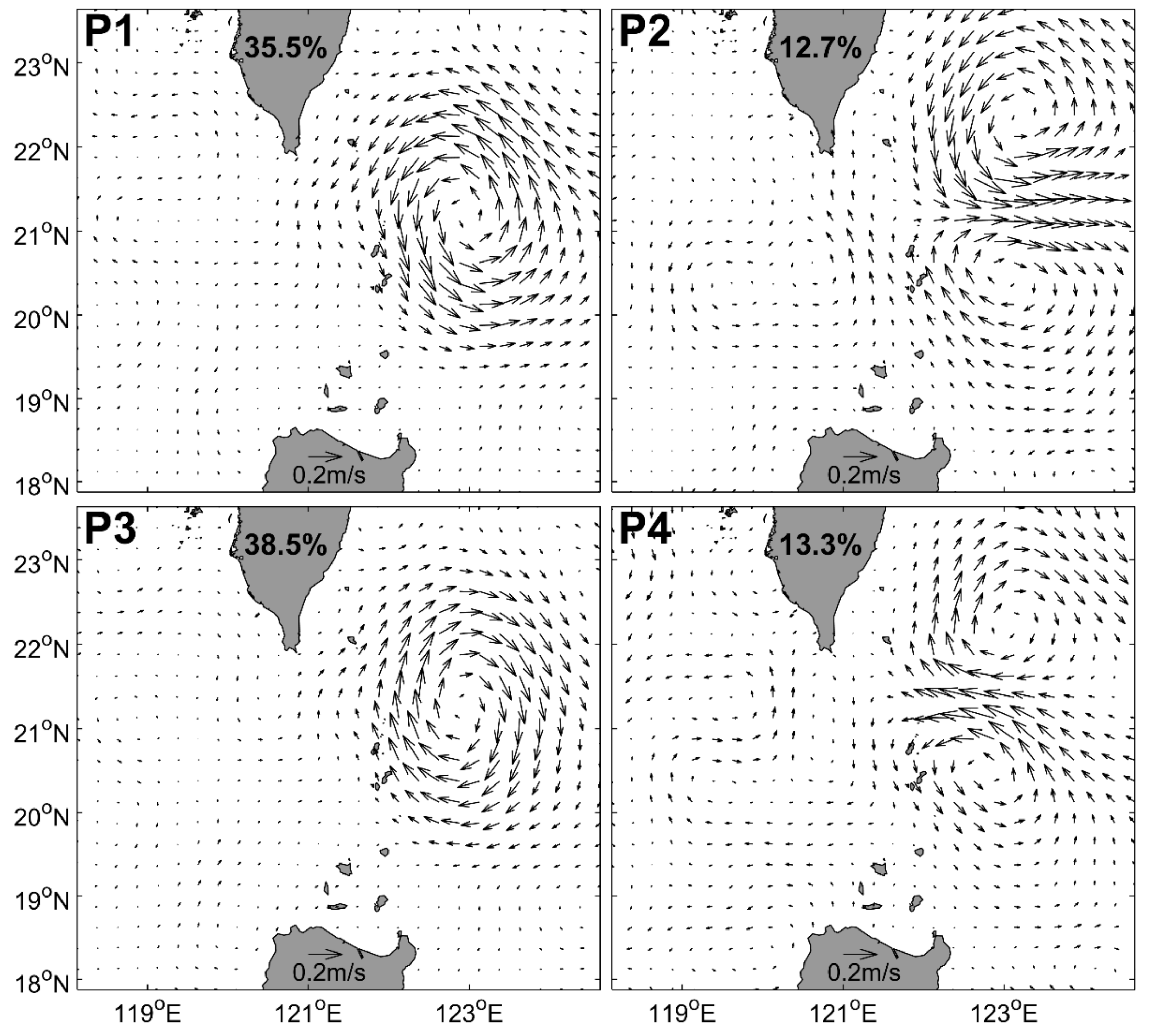
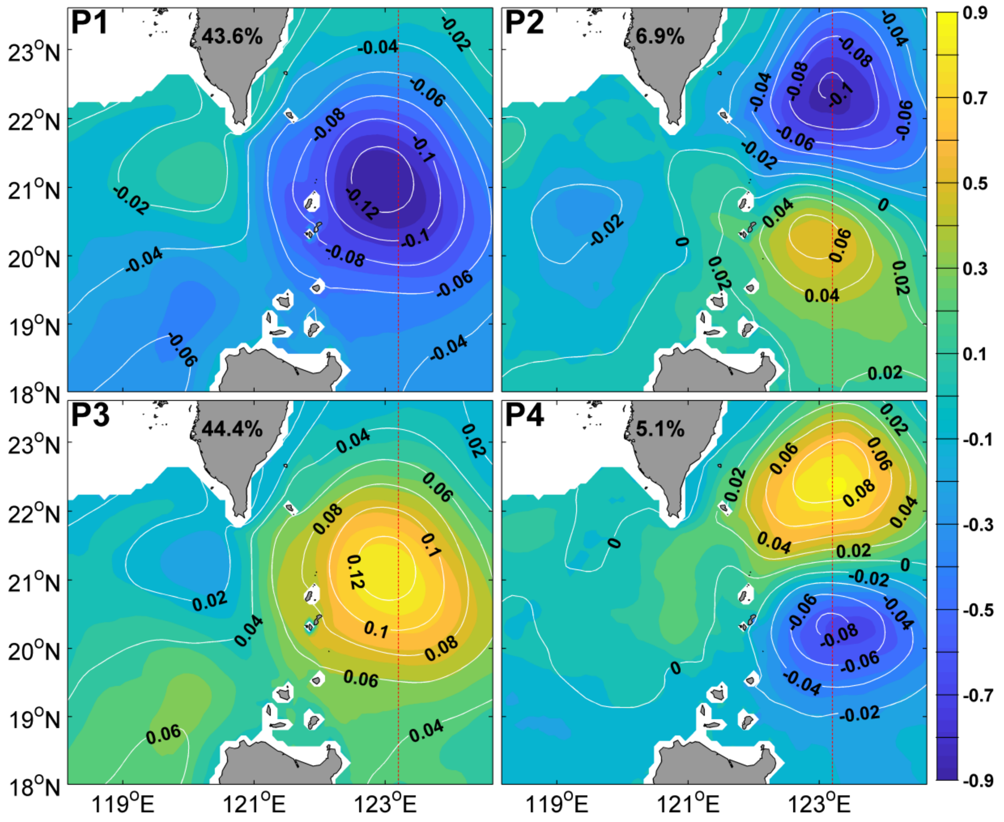
Applying the SOM method to the corresponding AVISO ADT data in the white box of Figure 1, we can obtain the dominant variation patterns of the east branch. Figure 2 shows that the east branch has four coherent patterns: anomalous southward (P1), anomalous eastward (P2), anomalous northward (P3), and anomalous westward (P4), which correspond to a cyclonic eddy (CE), CE-anticyclonic eddy (AE), an AE, and AE-CE to the east of the LS, respectively. Briefly, the four patterns of the east branch are dominated by single and dipole eddy structure, which is very similar to the SSH variability east of the Taiwan Island [33,34]. To the authors’ knowledge, the four patterns of the east branch in the LS have not been previously reported. P1 shows significantly southward velocity anomaly, which is caused by a CE to the east of LS. P2 shows significantly eastward velocity anomaly, which is accompanied by an eddy pair consisting of a CE on the north side of 21.2 °N and an AE on the south side of 21.2 °N. P3 is the opposite of P1, and is caused by an AE to the east of the LS. P4 is the opposite of P2, and is accompanied by an AE on the north side of 21.2 °N and a CE on the south side of 21.2 °N. The four patterns of the east branch also are identified in the HYCOM SSH data. Figure 3 shows that, P1 (P3) corresponds to a CE (an AE), and P2 (P4) corresponds to a CE (an AE) on the north side of 21.2 °N and an AE (a CE) on the south side of 21.2 °N, which corresponds well to the ones in Figure 2, although the occurrence rate of corresponding pattern of Figure 2 and Figure 3 is not exactly the same, which may be related to HYCOM model bias.

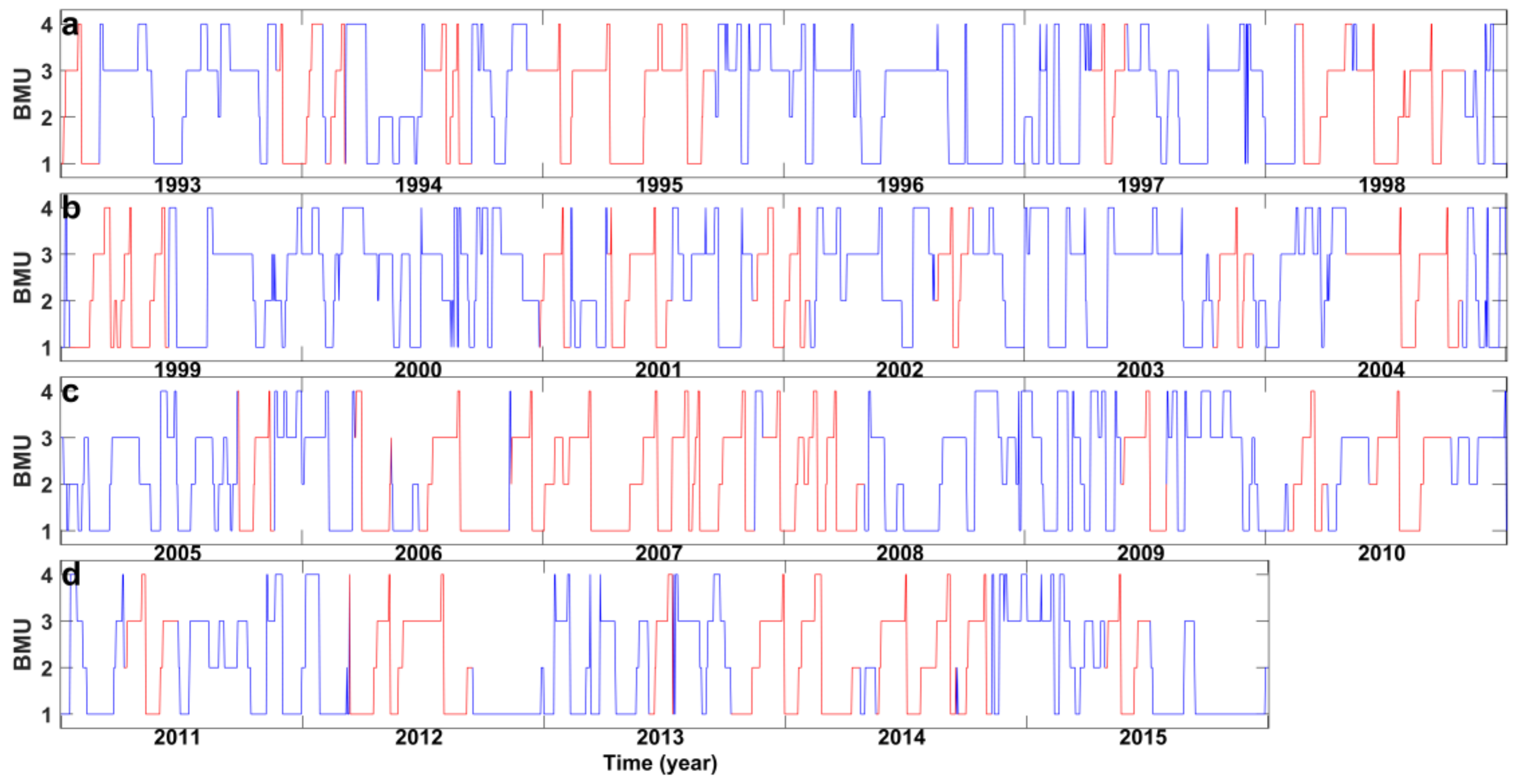
The temporal evolution of the four patterns can be seen from the time series of the BMU (Figure 4). The cycle characterized as a clockwise trajectory in the SOM space is very noteworthy, which has been marked by red lines in Figure 4. We take the cycle of P1, P2, P3, P4 and P1 as an example. First, a CE approaches from the east and weakens the east branch (P1). Second, as the CE flows northward and gradually weakens, an AE begins to form in the south (P2). Third, with the AE eddy strengthening, it approaches and enhances the east branch (P3). Finally, as the AE moves northward and gradually weakens, a CE in the south begins to form (P4). Note P1 as the initial pattern in the sequence is arbitrary. We define the occurrence of the preferred cycle by counting occurrences of clockwise trajectories that pass through all four patterns at least once. The percentage of time that follows the preferred cycle (red lines) to the total time analyzed is 39.2%.

Power spectrum analysis shows that the most significant cycle of the BMU is 62.2 days (Figure 5), which is consistent with the significant cycle of upper-layer and intermediate-layer transports based on observation data in the LS [35], and Zhang et al. pointed out that the ~60 days of variability might be attributed to the impinging mesoscale eddies from the Pacific [35]. The average consecutive days are 19.2, 6.0, 18.8, and 6.5 for P1, P2, P3, and P4, respectively, causing the total time length of a cycle of P1, P2, P3, and P4 to be between 56.5 days and 69.7 days, which is very close to 62.2 days. Therefore, we think that the cycle of the 62.2 days of the BMU is mainly caused by the cycle of P1, P2, P3, and P4.

3.2. The Effect of the Four Patterns on the Local Sea Temperature

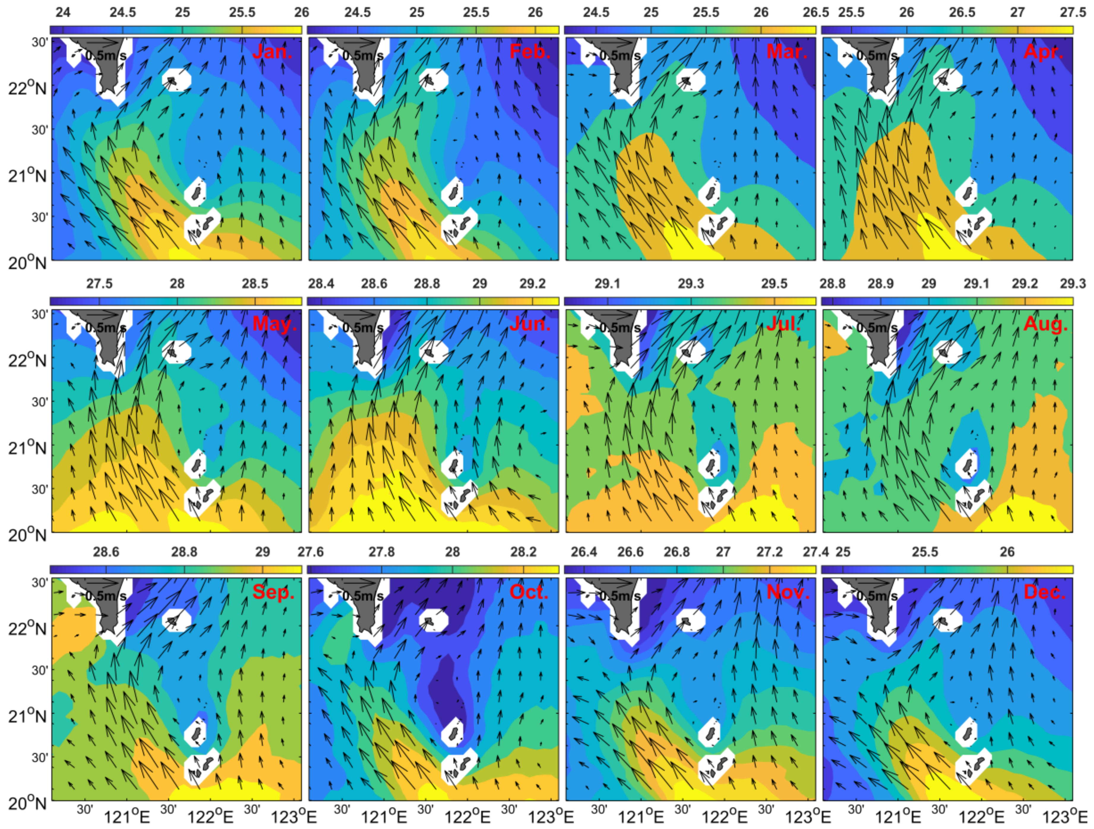
SST around the LS has obvious seasonal variability. Figure 6 shows that there is a good correspondence between the Kuroshio and warm tongues in most months, especially in winter, However, the Kuroshio fails to correspond well with warm tongues in some months such as in June and August. The high temperature in June and August is not conducive to the formation of warm tongue around the LS [32].

We apply a 4° moving average for RSS SST field for the purpose of removing the background state to highlight the effect of mesoscale process. Figure 7 shows that the four patterns of the east branch have a significant effect on SST around the LS. Sun et al. used a mixed-layer model based on temperature equation to demonstrate that the Kuroshio affects SST mainly through geostrophic thermal advection in the LS [14]. Through thermal advection, the east branch of the anomalous southward causes SST reduction in the location of the east branch (P1); the east branch of the anomalous eastward causes an eastward warm tongue (P2); P3 is the opposite of the P1, and SST increases in the location of the east branch (P3); P4 shows that the east branch of the anomalous westward causes a westward cold tongue. Figure 7 embodies that mesoscale eddies can influence sea temperature distribution by modulating the east branch of the Kuroshio of the western boundary current.

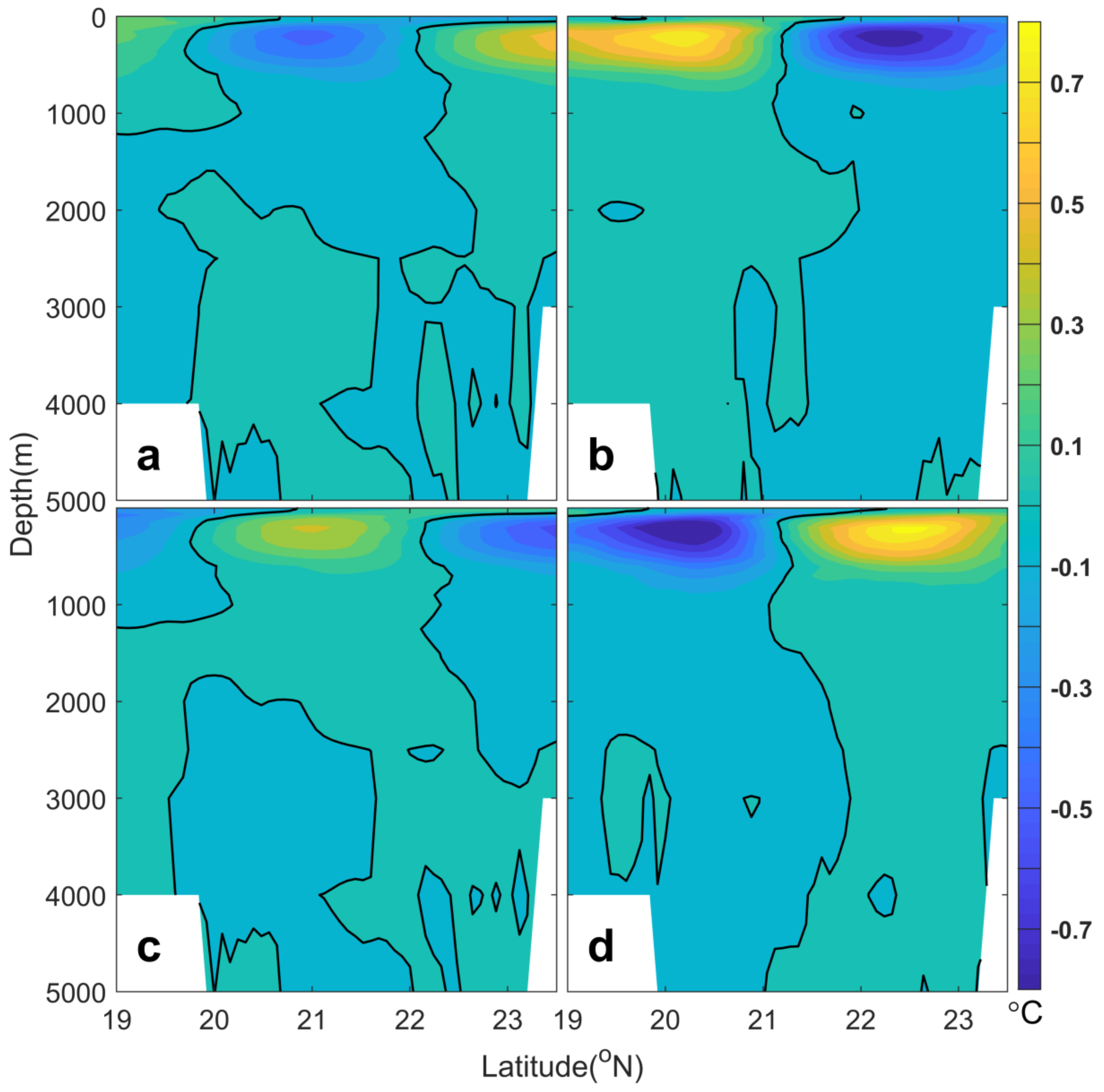
Besides affecting SST, the four patterns of the east branch can also affect deep sea temperature. Figure 3 shows that there is a good correspondence between sea temperature in 300 meters depth and the four patterns of the east branch: the CE (AE) corresponds to a cold (warm) center of sea temperature anomaly because of the following reasons. When the CE (AE) exists, SSHA is negative (positive) and upwelling (downwelling) occurs, and then the temperature in the deep ocean correspondingly decreases (increases) [36], which indicates that the four patterns of the east branch can affect the vertical distribution of sea temperature. Figure 8 gives vertical profile of sea temperature anomaly along the 123.2°E, which is marked as a red dotted line in Figure 3, and shows negative (positive) temperature anomaly corresponding to a CE (an AE) can reach 5000 meters deep. Based on Conductivity Temperature Depth (CTD) data, Zhang et al. found that mesoscale eddies can affect sea temperature in 2530 meters depth [36], and the conclusion in this paper is consistent with it in magnitude. However, based on HYCOM data in this paper, we found that the effect of the four patterns of the east branch on sea temperature can reach 5000 meters in depth, or even deeper [37].

4. Summary

Spatial patterns of the east branch of the Kuroshio bifurcation in the LS are extracted from the AVISO data and HYCOM data using the method of SOM. Four coherent patterns are used to summarize the variation of the east branch: anomalous southward, anomalous eastward, anomalous northward, and anomalous westward, which corresponds to a CE, CE-AE, an AE, and AE-CE to the east of the LS, respectively. The robust clockwise cycle of the four patterns causes a 62.2 days cycle of the east branch.

The four patterns of the east branch modulated by mesoscale eddies can influence horizontal and vertical distribution of local sea temperature. East branch of anomalous southward (northward) causes SST reduction (increase) in the location of east branch. East branch of anomalous eastward causes an eastward warm tongue while east branch of anomalous westward causes a westward cold tongue. The effect of the four patterns of the east branch on sea temperature can reach 5000 meters deep.

The patterns of the east branch of the Kuroshio bifurcation and their temporal evolution, as revealed by the SOM, provide new insights into the variability of the Kuroshio and their effect on the local sea temperature. Detailed dynamic mechanism studies with numerical models and more in situ observations are warranted as part of future work.

References

- Tokinaga, H.; Tanimoto, Y.; Xie, S.; Sampe, T.; Tomita, H.; Ichikawa, H. Ocean frontal effects on the vertical development of clouds over the Western North Pacific: In situ and satellite observations. J. Clim. 2009, 22, 4241–4260. [Google Scholar] [CrossRef]
- Kelly, K.A.; Small, R.J.; Samelson, R.M.; Qiu, B.; Joyce, T.M.; Kwon, Y.-O.; Meghan, F.C. Western boundary currents and frontal air-sea interaction: Gulf stream and Kuroshio extension. J. Clim. 2010, 23, 5644–5667. [Google Scholar] [CrossRef]
- Qiu, B.; Chen, S.; Schneider, N.; Taguchi, B. A coupled decadal prediction of the dynamic state of the Kuroshio extension system. J. Clim. 2014, 27, 1751–1764. [Google Scholar] [CrossRef]
- Guo, L.; Xiu, P.; Chai, F.; Xue, H.; Wang, D.; Sun, J. Enhanced chlorophyll concentrations induced by Kuroshio intrusion fronts in the northern South China Sea. Geophys. Res. Lett. 2017, 44, 11565–11572. [Google Scholar] [CrossRef]
- Zhou, P.; Song, X.; Yuan, Y.; Wang, W.; Cao, X.; Yu, Z. Intrusion pattern of the Kuroshio Subsurface Water onto the East China Sea continental shelf traced by dissolved inorganic iodine species during the spring and autumn of 2014. Mar. Chem. 2017, 196, 24–34. [Google Scholar] [CrossRef]
- Waseda, T. On the Eddy-Kuroshio interaction: Meander formation process. J. Geophys. Res. 2003, 108, 3220. [Google Scholar] [CrossRef]
- Sheu, W.; Wu, C.; Oey, L. Blocking and westward passage of eddies in the Luzon Strait. Deep. Sea. Res. 2010, 57, 1783–1791. [Google Scholar] [CrossRef]
- Zheng, Q.; Tai, C.; Hu, J.; Lin, H.; Zhang, R.-H.; Su, F.-C.; Yang, X. Satellite altimeter observations of nonlinear Rossby Eddy-Kuroshio interaction at the Luzon Strait. J. Oceanogr. 2011, 67, 365–376. [Google Scholar] [CrossRef]
- Lu, J.; Liu, Q. Gap-leaping Kuroshio and blocking westward-propagating Rossby wave and eddy in the Luzon Strait. J. Geophys. Res. 2013, 118, 1170–1181. [Google Scholar] [CrossRef] [Green Version]
- Cheng, Y.; Ho, C.; Zheng, Q.; Qiu, B.; Hu, J.; Kuo, N.-J. Statistical features of eddies approaching the Kuroshio east of Taiwan Island and Luzon Island. J. Oceanogr. 2017, 73, 1–12. [Google Scholar] [CrossRef]
- Zhang, Z.; Zhao, W.; Qiu, B.; Tian, J. Anticyclonic eddy sheddings from Kuroshio Loop and the accompanying cyclonic eddy in the northeastern South China Sea. J. Phys. Oceanogr. 2017, 47, 1243–1259. [Google Scholar] [CrossRef]
- Wang, G.; Wang, D.; Zhou, T. Upper layer circulation in the Luzon Strait. Aquat. Ecosyst. Health 2012, 15, 39–45. [Google Scholar] [CrossRef] [Green Version]
- Jia, Y.; Liu, Q. Eddy shedding from the Kuroshio Bend at Luzon Strait. J. Oceanogr. 2004, 60, 1063–1069. [Google Scholar] [CrossRef]
- Sun, R.; Wang, G.; Chen, C. The Kuroshio bifurcation associated with islands at the Luzon Strait. Geophys. Res. Lett. 2016, 43, 5768–5774. [Google Scholar] [CrossRef]
- Sun, R.; Gu, Y.; Li, P.; Li, L.; Zhai, F.; Gao, G. Statistical characteristics and formation mechanism of the Lanyu cold eddy. J. Oceanogr. 2016, 72, 641–649. [Google Scholar] [CrossRef]
- Ho, C.-R.; Zheng, Q.; Kuo, N.-J.; Tsai, C.-H.; Huang, N.E. Observation of the Kuroshio intrusion region in the South China Sea from AVHRR data. Int. J Remote. Sens. 2004, 25, 4583–4591. [Google Scholar] [CrossRef]
- Caruso, M.J.; Gawarkiewicz, G.G.; Beardsley, R.C. Interannual variability of the Kuroshio intrusion in the South China Sea. J. Oceanogr. 2006, 62, 559–575. [Google Scholar] [CrossRef]
- Nan, F.; Xue, H.; Chai, F.; Shi, L.; Shi, M.; Guo, P. Indentification of different types of Kuroshio intrusion into the South China Sea. Ocean. Dynam. 2011, 61, 1291–1304. [Google Scholar] [CrossRef]
- Nan, F.; Xue, H.; Yu, F. Kuroshio intrusion into the South China Sea: A review. Prog. Oceanogr. 2015, 137, 314–333. [Google Scholar] [CrossRef]
- Ducet, N.; Traon, P.Y.; Reverdin, G. Global high-resolution mapping of ocean circulation from TOPEX/Poseidon and ERS-1 and-2. J. Geophys Res. 2000, 105, 19477–19498. [Google Scholar] [CrossRef]
- Duacs. A New Version of SSALTO/Duacs Products Available in April 2014; Duacs: Toulouse, France, 2014. [Google Scholar]
- Jin, B.; Wang, G.; Liu, Y.; Zhang, R. Interaction between the East China Sea Kuroshio and the Ryukyu Current as revealed by the self-organizing map. J. Geophys. Res. 2010, 115. [Google Scholar] [CrossRef] [Green Version]
- Kohonen, T. Self-Organizing Maps; Vol. of 30 Springer Series in Information Sciences, 3rd ed. Springer: Berlin, Germany, 2001; p. 501. [Google Scholar]
- Hsieh, W.W. Non-linear principal component analysis by neural networks. Tellus A 2001, 53, 599–615. [Google Scholar] [CrossRef]
- Hsieh, W.W. Nonlinear multivariate and time series analysis by neural network methods. Rev. Geophys. 2004, 42. [Google Scholar] [CrossRef] [Green Version]
- Liu, Y.; Weisberg, R.H. Patterns of ocean current variability on the West Florida Shelf using the self-organizing map. J. Geophys. Res. 2005, 110. [Google Scholar] [CrossRef] [Green Version]
- Liu, Y.; Weisberg, R.H.; Mooers, C.N. Performance evaluation of the self-organizing map for feature extraction. J. Geophys. Res. 2006, 111, 1–14. [Google Scholar] [CrossRef]
- Cavazos, T. Using self-organizing maps to investigate extreme climate events: An application to wintertime precipitation in the Balkans. J. Clim. 2000, 13, 1718–1732. [Google Scholar] [CrossRef]
- Iskandar, I.; Tozuka, T.; Masumoto, Y.; Yamagata, T. Impact of Indian Ocean Dipole on intraseasonal zonal currents at 90° E on the equator as revealed by self-organizing map. Geophys. Res. Lett. 2008, 35. [Google Scholar] [CrossRef]
- Johnson, N.C. How many ENSO flavors can we distinguish? J. Clim. 2013, 26, 4816–4827. [Google Scholar] [CrossRef]
- Yin, Y.; Lin, X.; Li, Y. Seasonal variability of Kuroshio intrusion northeast of Taiwan Island as revealed by self-organizing map. Chin. J. Oceanol. Limnol. 2014. [Google Scholar] [CrossRef]
- Sun, R. The Ocean Dynamics and Its effect on the sea temperature near the Luzon Strait. Ph.D. Thesis, Ocean University of China, Qingdao, China, December 2015. (In Chinese). [Google Scholar]
- Hsin, Y.; Qiu, B.; Chiang, T.; Wu, C.-R. Seasonal to interannual variations in the intensity and central position of the surface Kuroshio east of Taiwan. J. Geophys. Res. 2013, 118, 4305–4316. [Google Scholar] [CrossRef] [Green Version]
- Yan, X.; Zhu, X.; Pang, C.; Zhang, L. Effects of mesoscale eddies on the volume transport and branch pattern of the Kuroshio east of Taiwan. J. Geophys. Res. 2016, 121, 7683–7700. [Google Scholar] [CrossRef]
- Zhang, Z.; Zhao, W.; Tian, J.; Yang, Q.; Qu, T. Spatial structure and temporal variability of the zonal flow in the Luzon Strait. J. Geophys. Res. 2015, 120, 759–776. [Google Scholar] [CrossRef] [Green Version]
- Zhang, Z.; Zhao, W.; Tian, J.; Liang, X. A mesoscale eddy pair southwest of Taiwan and its influence on deep circulation. J. Geophys. Res. 2013, 118, 6479–6494. [Google Scholar] [CrossRef] [Green Version]
- Zhang, Z.; Tian, J.; Qiu, B.; Zhao, W. Observed 3D structure, generation, and dissipation of oceanic mesoscale eddies in the South China Sea. Sci. Rep. 2016, 6, 24349. [Google Scholar] [CrossRef] [PubMed]
Figure 1.
Climatology of geostrophic current and sea surface temperature (SST) around the LS. The black line represents 27.2 °C, in order to emphasize the spatial patterns of two warm tongues. The white box covers 20.3° N–22° N, 121.875 °E–123.125 °E. Geostrophic current (m/s, in vector); SST (°C, in color); TWI: Taiwan Island; BIS: Batanes Islands; LZI: Luzon Island; SCS: South China Sea. The extent of the main map is shown as a black box in the inset.
Figure 2.
The 2 × 2 SOM patterns derived from the AVISO ADT fields for the east branch. Geostrophic current anomaly (m/s, in vector). The number on each panel represents the occurrence rate of corresponding pattern.
Figure 3.
The 2 × 2 SOM patterns derived from the HYCOM SSH fields for the east branch, and corresponding sea temperature anomaly in 300 meters deep. Sea Surface Height Anomaly (SSHA) (m, in contour); Sea temperature (°C, in color). The number on each panel represents the occurrence rate of corresponding pattern. The red dotted line represents meridional section of sea temperature, and its longitude is 123.2 °E.
Figure 4.
Time series of the BMU for the four patterns, as shown in Figure 2. On the y axis, 1, 2, 3 and 4 correspond to P1, P2, P3, and P4, respectively. The subgraphs (a), (b), (c), and (d) correspond to the period from 1993 to 1998, from 1999 to 2004, from 2005 to 2010, and from 2011 to 2015, respectively.
Figure 5.
Power spectrum analysis of time series of the BMU for the four patterns. The red dotted line represents the 95% significant level.
Figure 6.
Seasonal variability of SST and geostrophic current around the LS. SST (°C, in color); Geostrophic current (m/s, in vector).
Figure 7.
The spatial pattern of high-pass-filtered RSS SST corresponding to 2 × 2 SOM patterns derived from the AVISO ADT fields for the east branch. Geostrophic current anomaly (m/s, in vector); SST (°C, in color). The spatial filtering is done by subtracting a 4° moving average from the original RSS SST data to remove the large-scale background state. The black line represents a zero contour line.
Figure 8.
The profile of HYCOM temperature anomaly corresponding to the four patterns of the east branch. Subgraphs (a), (b), (c), and (d) correspond to P1, P2, P3 and P4 of the east branch patterns, respectively. The black line represents the zero contour line. It is noted that the zonal mean has been removed. Sea temperature (°C, in color).
© 2018 by the authors. Licensee MDPI, Basel, Switzerland. This article is an open access article distributed under the terms and conditions of the Creative Commons Attribution (CC BY) license (http://creativecommons.org/licenses/by/4.0/).
Share and Cite
MDPI and ACS Style
Sun, R.; Zhai, F.; Gu, Y. The Four Patterns of the East Branch of the Kuroshio Bifurcation in the Luzon Strait. Water 2018, 10, 1822. https://doi.org/10.3390/w10121822
AMA Style
Sun R, Zhai F, Gu Y. The Four Patterns of the East Branch of the Kuroshio Bifurcation in the Luzon Strait. Water. 2018; 10(12):1822. https://doi.org/10.3390/w10121822
Chicago/Turabian StyleSun, Ruili, Fangguo Zhai, and Yanzhen Gu. 2018. "The Four Patterns of the East Branch of the Kuroshio Bifurcation in the Luzon Strait" Water 10, no. 12: 1822. https://doi.org/10.3390/w10121822
Note that from the first issue of 2016, this journal uses article numbers instead of page numbers. See further details here.