Numerical Study of the Influence of Tidal Current on Submarine Pipeline Based on the SIFOM–FVCOM Coupling Model

Abstract

The interaction between coastal ocean flows and the submarine pipeline involved with distinct physical phenomena occurring at a vast range of spatial and temporal scales has always been an important research subject. In this article, the hydrodynamic forces on the submarine pipeline and the characteristics of tidal flows around the pipeline are studied depending on a high-fidelity multi-physics modeling system (SIFOM–FVCOM), which is an integration of the Solver for Incompressible Flow on the Overset Meshes (SIFOM) and the Finite Volume Coastal Ocean Model (FVCOM). The interactions between coastal ocean flows and the submarine pipeline are numerically simulated in a channel flume, the results of which show that the hydrodynamic forces on the pipeline increase with the increase of tidal amplitude and the decrease of water depth. Additionally, when scour happens under the pipeline, the numerical simulation of the suspended pipeline is also carried out, showing that the maximum horizontal hydrodynamic forces on the pipeline reduce and the vertical hydrodynamic forces grow with the increase of the scour depth. According to the results of the simulations in this study, an empirical formula for estimating the hydrodynamic forces on the submarine pipeline caused by coastal ocean flows is given, which might be useful in engineering problems. The results of the study also reveal the basic features of flow structures around the submarine pipeline and its hydrodynamic forces caused by tidal flows, which contributes to the design of submarine pipelines.

1. Introduction

For decades, much crude oil and natural gas have been found in the ocean, which are constantly mined and utilized with the development of marine science and technology. The exploited oil and gas are usually transported by submarine pipelines. Most of submarine pipelines are laid on the seabed and exposed to the various marine environments directly. The pipelines are strongly affected by forces from the complex marine environments such as unpredictable waves and currents. For example, due to the influence of the water flows, pipelines are prone to vibration damage or stress destruction in the deep sea, while pipelines are easily affected by coastal waves in shallow water. Pipeline accidents lead to not only huge economic losses but also serious marine environmental pollution because of crude oil leakage. In order to reduce accidents on submarine pipelines, it is necessary to carry out deep investigations on the interaction between tide-induced flows and submarine pipelines [1,2].

In the past, a series of studies about the submarine pipelines have been carried out experimentally and numerically. Through physical experiments, Kok [3] examined the locations of front stagnation and separation points on the pipeline as well as the magnitudes and directions of drag and lift forces, which gave a better understanding of various flow phenomena at the pipeline. Li et al. [4] experimentally studied the hydrodynamic force on a pipeline subjected to vertical seabed movement using an underwater shaking table, the results of which showed that the Reynolds number (Re) and Keulegan–Carpenter number (KC) are the two main parameters influencing the hydrodynamic force coefficients, known as the drag coefficient (C_D), added mass coefficient (C_A) and horizontal hydrodynamic force coefficient (C_V). Besides, the investigation of the influence of close proximity of a submarine pipeline to the seabed on the vortex-induced vibrations (VIV) of the pipeline was conducted by Yang et al. [5]. In the experiment, visualization of the flow field with hydrogen bubbles indicated that the wake vortexes became much more irregular with the decrease of the gap between the pipe and boundary. Mattioli et al. [6,7] investigated the near-bed dynamics around a submarine pipeline laying on different types of seabed under currents and waves, which revealed the mechanics of flow–sediment–pipeline interactions based on dedicated laboratory experiments.

Except for the experimental research, numerical simulations were also conducted to study the submarine pipeline. Pierro et al. [8] researched on the influence of boundary layer viscous dynamics on the lift and drag forces acting on a near-bed pipeline analytically and numerically. Investigation of high Reynolds number flows around a circular cylinder close to a flat seabed was conducted by Ong et al. [9] using a two-dimensional standard high Reynolds number κ-ε model. It was found that the time-averaged drag coefficient (C_D) of the cylinder increased as the gap between pipeline and a seabed flat to pipeline diameter ratio (G/D) increased for small G/D. Cheng and Chew [10] studied the effect of a spoiler on flow around the pipeline and the seabed. An additional spoiler on top of a pipe would substantially increase the pressure on the upstream of the pipe and decrease the base pressure at the back of the pipe. Reviews of this subject also can be found in many published papers [11,12,13,14,15,16,17,18,19,20]. In these studies, hydrodynamic forces on pipelines were induced by viscosity, inertia, flow asymmetry and vortex shedding, while analytical expressions were proposed for the evaluation in some cases.

Although many investigations have been conducted experimentally and numerically on hydrodynamics at submarine pipelines, the research focuses on the unidirectional steady flow in small scale flow field rather than realistic ocean environment. The past studies ignored the strong interaction between small- and large-scale phenomena. Spatially, the real sea area is much larger than the area near the submarine pipeline, indicating that the simulation accuracy of the large-scale model can hardly satisfy the simulation of a small-scale structure. In the meanwhile, although the simulation accuracy of small-scale models might meet with the simulation requirement of the submarine pipeline, they are not able to calculate the large-scale ocean model due to the limitation of calculation conditions. Temporally, the period of regular semi-diurnal tide is usually 12 h, leading to a large ratio of the time scale of ocean model against the small-scale model; therefore, the small-scale model cannot be used to simulate tidal flows accurately which oscillate in a much longer period. Since one of the major tasks in the design of submarine pipelines is the analysis of hydrodynamic stability, it is crucial to ensuring that during construction and operation stages, the pipelines are able to remain stable under the action of hydrodynamic forces induced by tidal currents and waves [21].

Due to the drawbacks of the existing references and the deficiency of hydrodynamic simulation for submarine pipelines, a multi-physics/multi-scale approach is indispensable for the accurate simulation of the interaction between flows and pipelines, which has become an important subject in the prediction of coastal ocean flows in recent years [22]. In this research, the Solver for Incompressible Flow on Overset Meshes (SIFOM) and the Unstructured Grid Finite Volume Coastal Ocean Model (FVCOM) [23] are interactively combined as one system to carry out numerical simulations of the interaction between flows and pipelines and study the hydrodynamic forces acting on pipelines, in which the SIFOM is used to calculate small-scale local hydrodynamics around the submarine pipeline, and the FVCOM is employed to capture large-scale coastal ocean tidal currents. SIFOM–FVCOM can solve the incompatibility problems of different scale models according to the domain decomposition method. Besides, the data between SIFOM and FVCOM exchange in the nested meshes directly and march in time simultaneously, which omits the steps of data storage and readout between different models. The calculation time of the coupling model is shortened greatly which can provide predictive results quickly for the engineering practice. Besides, FVCOM as a marine prediction model has been used popularly to forecast the marine environment. So, this model also can predict the realistic coastal flow around the ocean and coastal engineering depending on the present marine conditions to achieve the purpose of the disaster prevention.

The structure of this paper is organized as follows. Firstly, the modeling system is briefly introduced in Section 2, while validations of the system are given in Section 3. Secondly, systematic simulations of the interaction between flows and pipelines are carried out in a numerical channel, the results of which are analyzed with regard to flow structures and hydrodynamic forces in Section 4. Meaningful conclusions of the study and some discussions are listed in Section 5.

2. Solver for Incompressible Flow on Overset Meshes–Unstructured Grid Finite Volume Coastal Ocean Model (SIFOM–FVCOM) Modeling System

In order to simulate the realistic multi-physics/multi-scale ocean phenomena, the domain decomposition approach is adopted in SIFOM–FVCOM, and the solution data exchange among different overset grids.

2.1. SIFOM Modeling

In the SIFOM modeling, the Cartesian coordinate is used as a reference system and the mesh in this model is divided into rectangular grids for the calculation. The I-, J- and K-directions of the rectangular grids are corresponding to the x-, y- and z-directions of the Cartesian coordinate, respectively. The mass and momentum conservation equations are employed to govern three-dimensional flow motion, and Chimera grids and the Schwarz alternative iteration are used in the modeling. The governing equations are as follows:

$$\nabla ·\mathbf{u}=0$$

(1)

where ∇ is the gradient operator; u is the velocity vector.

$${\mathbf{u}}_t+\nabla ·\mathbf{uu}=-\frac{1}{{\rho }_0}\nabla p_d+\nabla ·((\nu +{\nu }_t)\nabla \mathbf{u})-g{\nabla }_H\zeta +g(\alpha (T-T_0)-\beta (C-C_0))\mathbf{k}$$

(2)

where t is time; ρ₀ is the reference density; p_d is the dynamic pressure; ν is the fluid viscosity; ν_t is the turbulence viscosity; g is the gravity; ∇_H is the horizontal gradient operator; ζ is the water surface elevation; α is the thermal expansion coefficient; T is the temperature; T₀ is a reference temperature; β is a coefficient reflecting the expansion; C is the tracer concentration; C₀ is a reference concentration; k is the unit vector in the vertical direction.

A second-order accurate, implicit, finite-difference method is used on non-staggered, curvilinear grids. The QUICK scheme [24] is used to discretize convective terms. The odd-even decoupling of the pressure field is eliminated by a third-order, fourth-order difference artificial dissipation method [25].

2.2. FVCOM Modeling

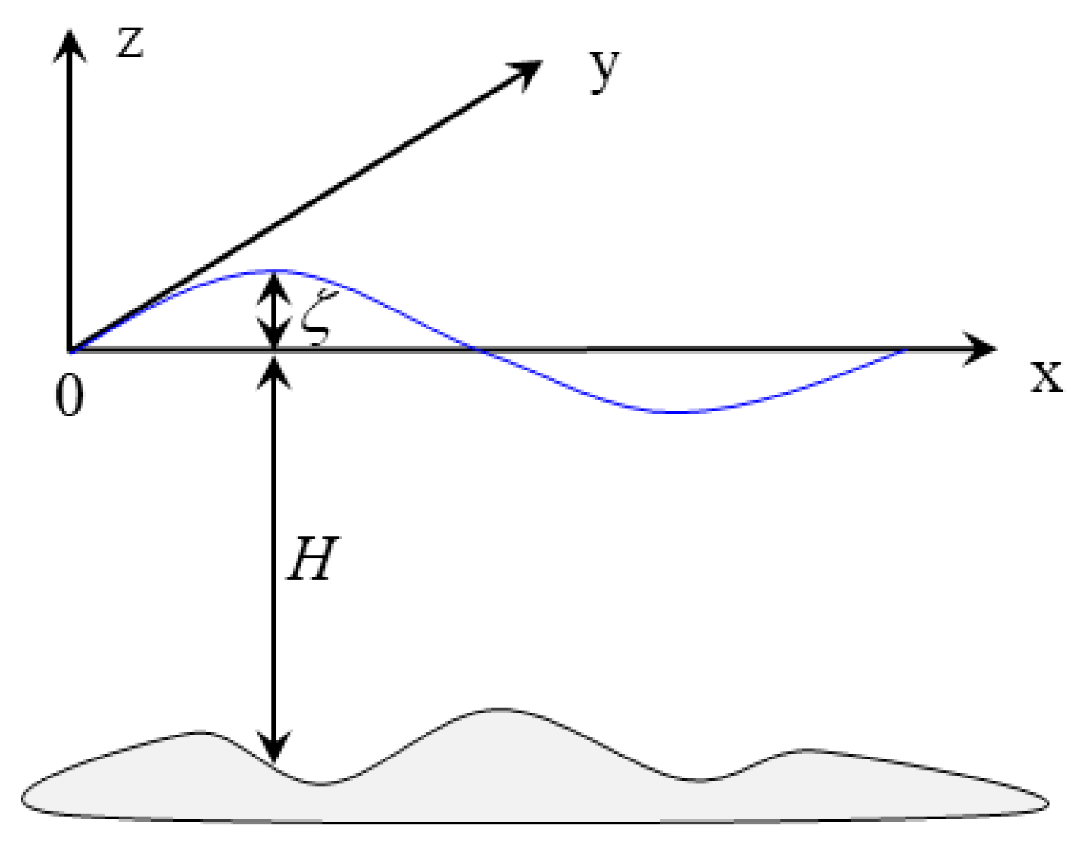
FVCOM is a geophysical fluid dynamics model. The unstructured/triangle mesh is used in the horizontal plane to deal with complicate coastlines. In the vertical direction, in order to obtain a smooth representation of irregular bottom topography in the ocean, all equations are transformed into σ coordinate from z coordinate of the Cartesian coordinate. The coordinate transformation expression is written as follows:

$$\sigma =\frac{z-\zeta }{H+\zeta }=\frac{z-\zeta }{D}$$

(3)

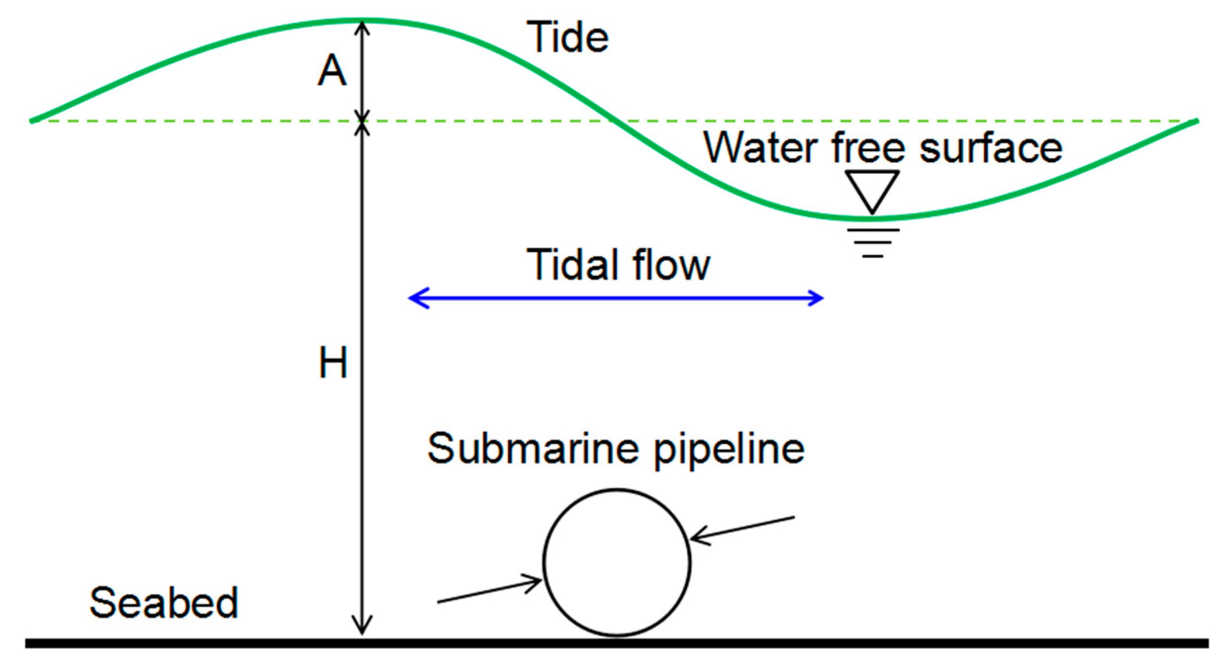
where z is the vertical position of a certain water level, ζ is the water surface elevation, H is the bottom depth and D is the total water column depth (Figure 1). The initial water surface is located at the z = 0 m and σ varies from −1 at the bottom to 0 at the surface. In the vertical direction of σ coordinate, the calculation domain is divided by many layers, which is referred to as σ-grids.

FVCOM consists of an external mode and an internal mode. Every mode includes continuity and momentum equations as the governing equations. A second-order accurate finite volume method is used in the model, which is able to preserve conservation of mass and momentum accurately. The governing equations of external mode are averaged governing equations in the σ-coordinate:

$${(\zeta )}_t+{\nabla }_H·(\mathbf{V}D)=0$$

(4)

$${\left(\mathbf{V}D\right)}_t+{\nabla }_H\cdot \left(\mathbf{VV}D\right)=-gD{\nabla }_H\zeta +\frac{{\mathbf{\tau }}_s-{\mathbf{\tau }}_b}{{\rho }_0}+\mathbf{G}$$

(5)

where V is the depth-averaged velocity vector; τ_b is the shear stress on the seabed; τ_s is the shear stress on the water surface; G includes Coriolis force and water friction force.

In the internal mode, the three dimensional governing equations are used based on the hydrostatic assumption:

$${(\zeta )}_t+{\nabla }_H·(\mathrm{V}D)+{(\omega )}_{\sigma }=0$$

(6)

$$\begin{array}{ll}{\left(\mathrm{V}D\right)}_t+{\nabla }_H·\left(\mathrm{VV}D\right)+{\left(V\omega \right)}_{\sigma }=& -gD{\nabla }_H\zeta +{\nabla }_H·\left(\kappa \mathbf{e}\right)+{\left(\lambda {\mathbf{V}}_{\sigma }\right)}_{\sigma }/D+H\\ & -\frac{gD}{{\rho }_o}\left({\nabla }_H\left(D{\displaystyle {\int }_{\sigma }^0\rho d{\sigma }^{\prime }}\right)+\sigma \rho {\nabla }_{H}D\right)\end{array}$$

(7)

where V is the horizontal velocity; ω is the vertical velocity in σ coordinate; e is the strain rate; H stands for the residual terms; κ and λ are coefficients.

In the two modes of FVCOM, the time derivative terms are discretized by the Runge–Kutta method, and the convection terms are discretized using upwind schemes [26].

2.3. Coupling Strategy of SIFOM–FVCOM Modeling

From the above discussion of the SIFOM and FVCOM, it demonstrates that two models are different in computational meshes, governing equations and numerical algorithms. In order to simulate the multi-physics/multi-scale ocean flow, the SIFOM and FVCOM must be integrated using a coupling strategy, which is presented in this section.

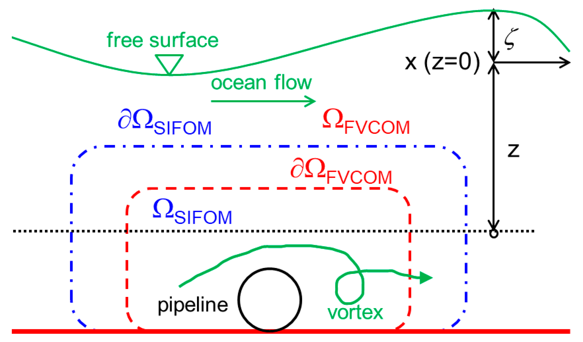
The sketch of the devised domains around the submarine pipeline is shown in Figure 2. The models of SIFOM and FVCOM overlap around the submarine pipeline. Ω_SIFOM and Ω_FVCOM are the calculation domains of SIFOM and FVCOM, respectively. The boundaries of ∂Ω_SIFOM and ∂Ω_FVCOM are the interfaces of SIFOM and FVCOM, respectively. Ω_SIFOM-FVCOM is the zone of SIFOM enclosed between the seabed and the red dashed line of ∂Ω_FVCOM. In the overlap domain, SIFOM and FVCOM exchange solutions at the interfaces of ∂Ω_SIFOM and ∂Ω_FVCOM.

The velocity u of SIFOM are the same as the velocity u(V, ω) of FVCOM. The velocity values are exchanged from FVCOM to SIFOM at the interfaces.

$${\mathbf{u}}_{SIFOM}={\mathbf{u}}_{FVCOM},on\partial {\Omega }_{SIFOM}$$

(8)

Due to the change of water level and velocity, the pressures in a domain of SIFOM includes the static pressure and hydrodynamic pressure.

$$p={\rho }_{0}g(\zeta -z)+p_d$$

(9)

where z is vertical position of a certain water level.

When the solutions of SIFOM exchange to FVCOM, similar conditions are adopted:

$${\mathbf{u}}_{FVCOM}={\mathbf{u}}_{SIFOM},on\partial {\Omega }_{FVCOM}$$

(10)

In these conditions, the solution exchange from the SIFOM to FVCOM is also conducted in the domain of Ω_SIFOM-FVCOM which is called the blanket zone. In this way, the structure of FVCOM does not need to be modified around the submarine pipeline. In the blanked zone, the solution values are redistributed and interpolated on the domain of FVCOM.

$${\mathbf{u}}_{FVCOM}={\mathbf{u}}_{SIFOM},on\partial {\Omega }_{SIFOM-FVCOM}$$

(11)

The coupling solving process between SIFOM and FVCOM can be seen in the Appendix.

3. Modeling System Validation

Depending on the investigation data of DF1-1 submarine pipeline off the west coast of Dongfang, Hainan Island, the measured maximum near-bed current velocity varies between 0.40 m/s and 0.91 m/s and the submarine pipeline diameter changes from 0.30 m to 1.60 m [27]. It is noted that when the submarine pipeline lays on the seabed, due to the influence of the seabed boundary layer on the tidal flow, the velocity around the pipeline is not so much that the Reynolds numbers are in the supercritical flow regime. Based on this prototype conditions, in order to ensure the SIFOM–FVCOM modeling system works appropriately, three flows are simulated and the results are compared with existing experimental data.

3.1. Validation on Flow Velocity and Vortex

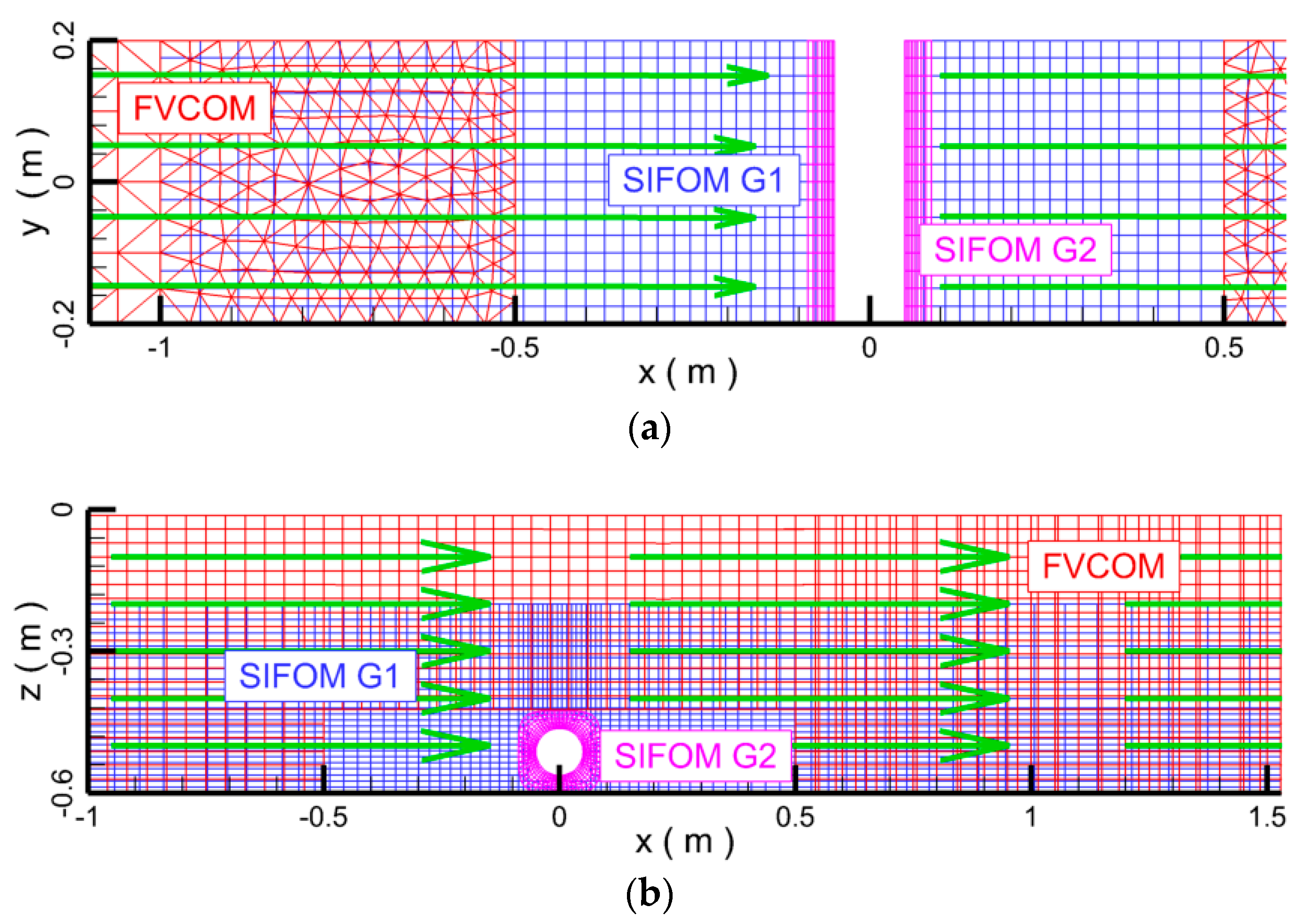
The first test is that a steady current passes a cylinder which is suspended above the ground. The flow parameters employed in the computation are the same as those in the experiments by Jensen [28]. The total water depth is 0.6 m and Reynolds number is 7000 which is based on the incoming velocity of 0.07 m/s and pipeline diameter of 0.1 m. The ratio of the gap between the bottom and pipeline to the pipeline diameter is 0.37. The cylinder center was placed at (x, y) = (0 m, −0.513 m). In the simulation, a rectangular flow domain is considered. The length and width of the calculation domain are 10 m and 5 m, respectively. SIFOM encloses the region near the pipeline, while FVCOM covers the region away from it. There are two sets of meshes (G1 and G2) in SIFOM and one set of meshes in FVCOM (Figure 3). The grid layer is nested, and the density of the grid is increasing from the far field to the pipeline and seabed.

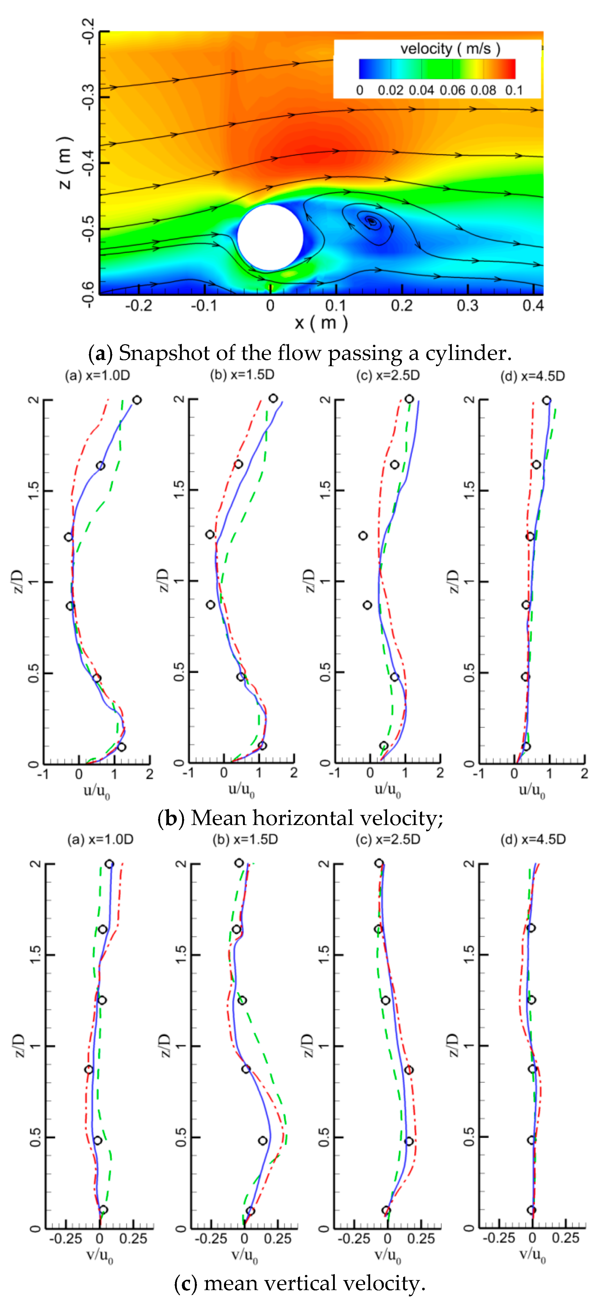
Due to the disturbance of the cylinder, the flow behind the cylinder is unsteady (Figure 4). The mean horizontal and vertical velocities of instantaneous solutions are presented in Figure 4b,c, respectively. It is seen that there is little difference between the results modeled by SIFOM alone and SIFOM–FVCOM, which is attributed to the fact that the top boundary of the computational domain is considered a rigid plane using SIFOM alone, whereas the one using SIFOM–FVCOM is treated as a free surface. Besides, the coupling strategy between SIFOM and FVCOM might leads to small errors. In short, the results obtained with SIFOM–FVCOM system agree reasonably with computational and experimental results in the literature.

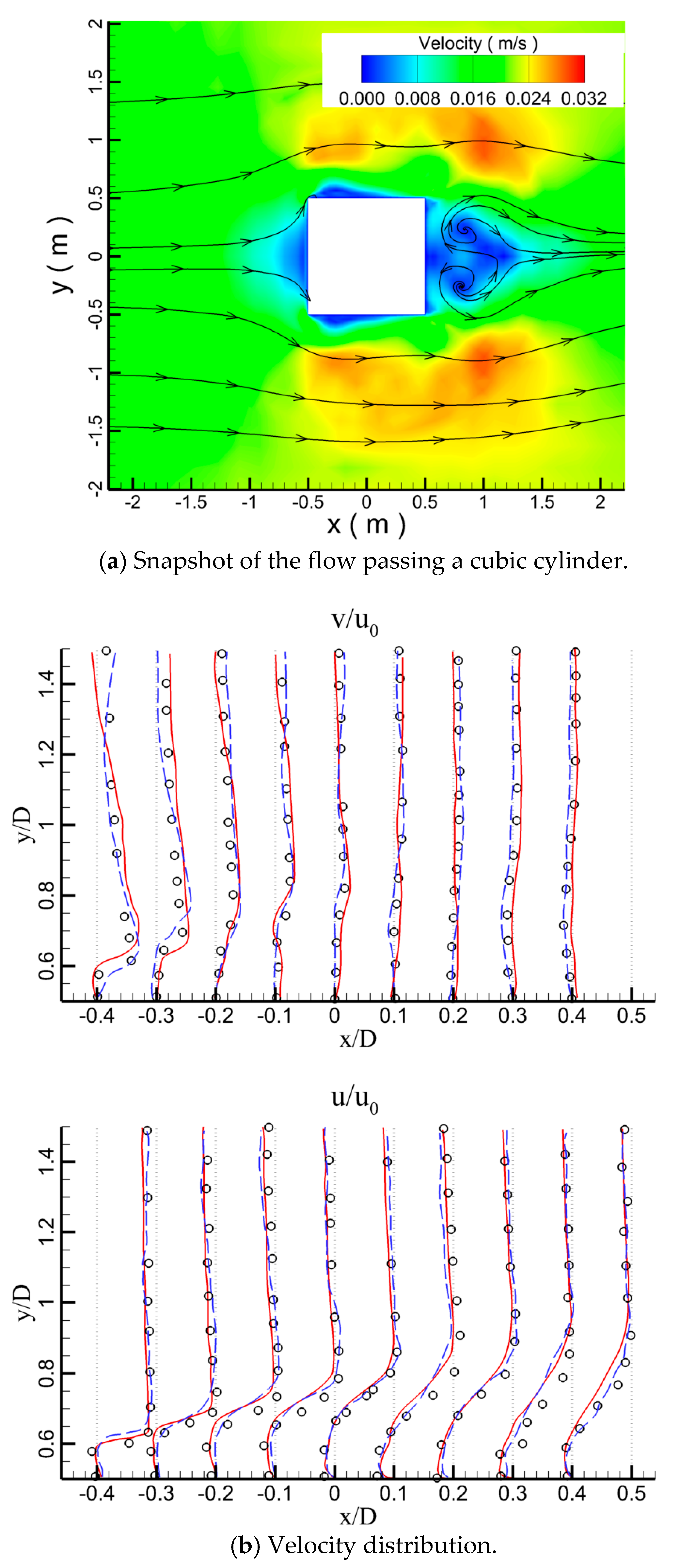
The second test is a 3D flow passes a square cylinder at bottom of a channel. The length and width of the channel are 54 m and 30 m, respectively. The water depth is 3.14 m and Reynolds number is 21,400 which is based on the incoming velocity of 0.02 m/s and the square length of 1 m. The flow field around the square cylinder is shown in Figure 5a, which is simulated by the SIFOM–FVCOM system. The result of SIFOM–FVCOM in Figure 5b is an average of instantaneous solution over time. The comparison of the velocity distribution also shows that the SIFOM–FVCOM system produces results that agree well with existing data in the literature.

3.2. Validation on Force

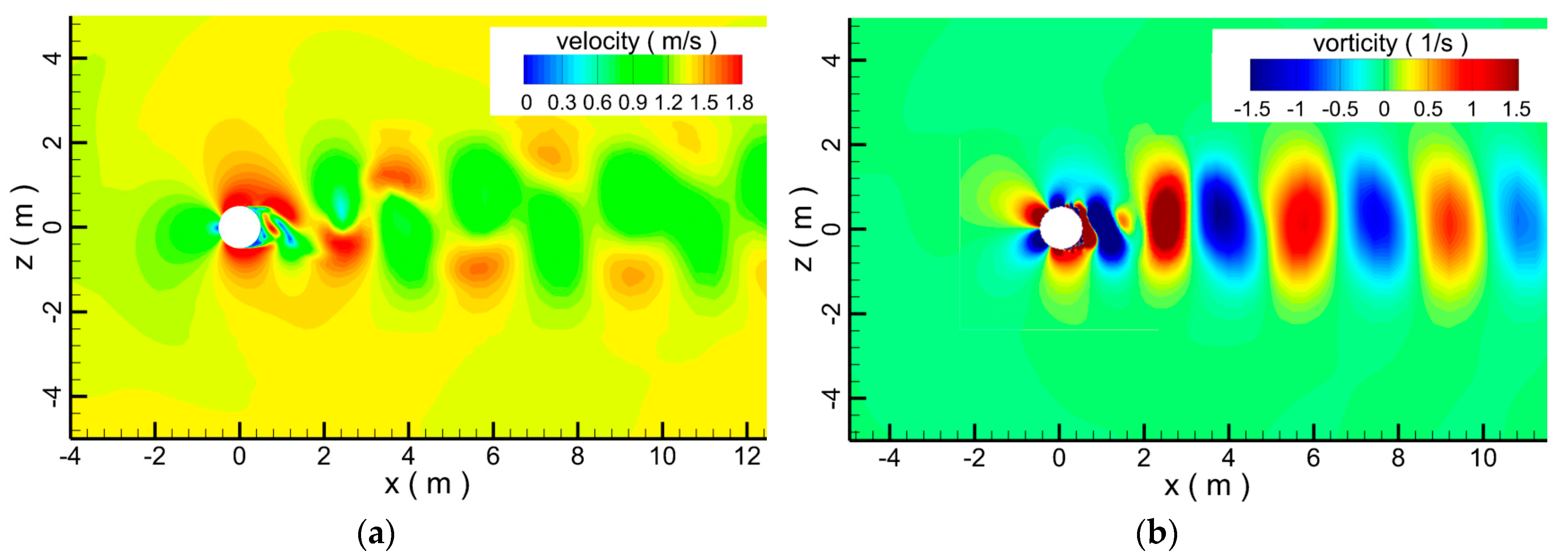
In order to ensure the accuracy of the simulation, validation on force is also necessary, which is the case of the flow crossing a circular cylinder with the Re = 1.2 × 10⁶. The velocity of incoming steady current is about 1.2 m/s. The water depth is about 10 m. The pipeline diameter is 1.0 m. The flow field and vorticity field around the pipeline simulated by SIFOM–FVCOM system are drawn in Figure 6, indicating that the vortex behind the pipeline is shedding periodically.

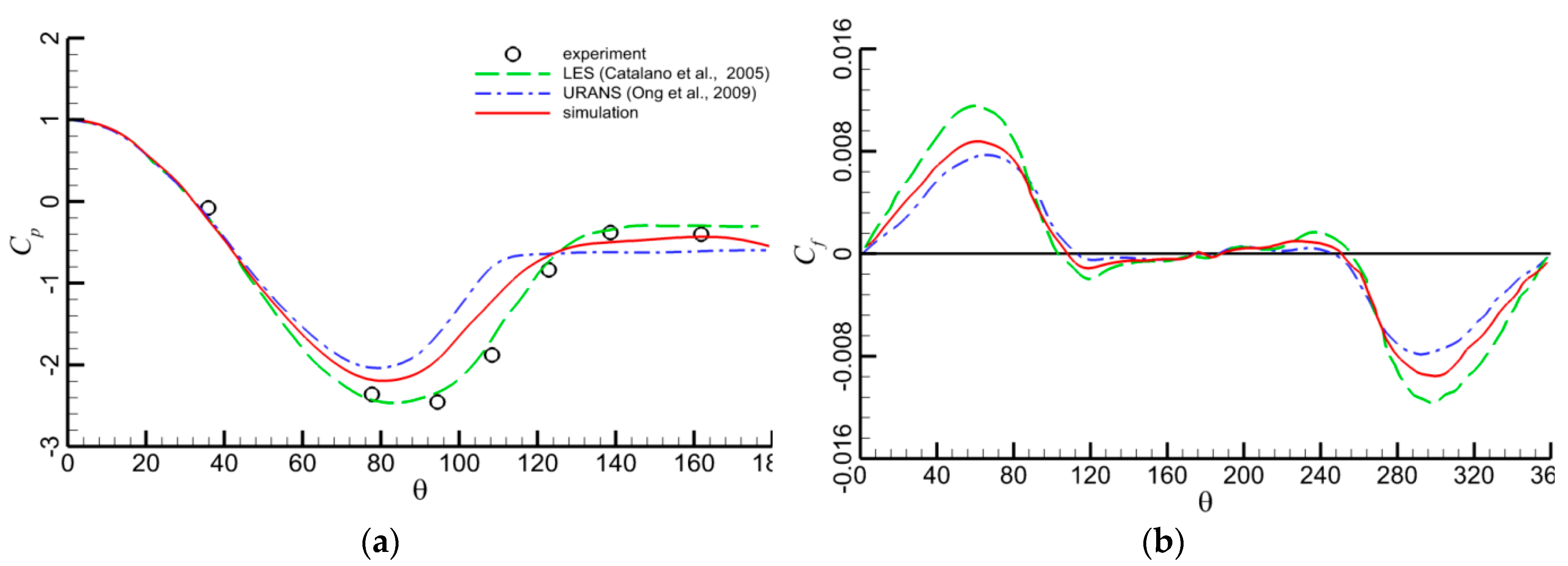
Figure 7a displays the predicted mean pressure distribution (C_p = (p_c − p_c∞)/(0.5ρU²_∞)), compared with the experimental data and simulation results. Here, p_c is the static pressure at the peripheral angle θ of the cylinder, and θ is clockwise angle from the stagnation point. p_c∞ is the static pressure of the flow at infinity. The predictions of the skin friction coefficient (C_f = τ/(0.5ρU²_∞)) are shown in Figure 7b. Here, τ is the tangential wall shear stress. In the figures, the simulation data are collected by the SIFOM–FVCOM system. The 3D LES and URANS results [9,31] are plotted for comparison. It is well known that the flow in the separation point region has a strong pressure gradient, and there is little difference between simulation and experimental results. In short, the simulation results agree well with the measurements around the cylinder.

4. Results and Discussions

4.1. Hydrodynamics around Submarine Pipeline with No Scour

In this section, the hydrodynamics around the submarine pipeline with no scour is studied based on the SIFOM–FVCOM coupling model. The influence of different pipeline diameters, tidal amplitudes and water depths on the flow structure and hydrodynamic forces on the pipeline is also researched. According to the research results, empirical formulas of hydrodynamic forces under tidal flows are proposed.

4.1.1. The Mesh and Calculation Setting

In order to understand the hydrodynamics at submarine pipelines in tidal flows, a modeling study has been made for a problem depicted in Figure 8.

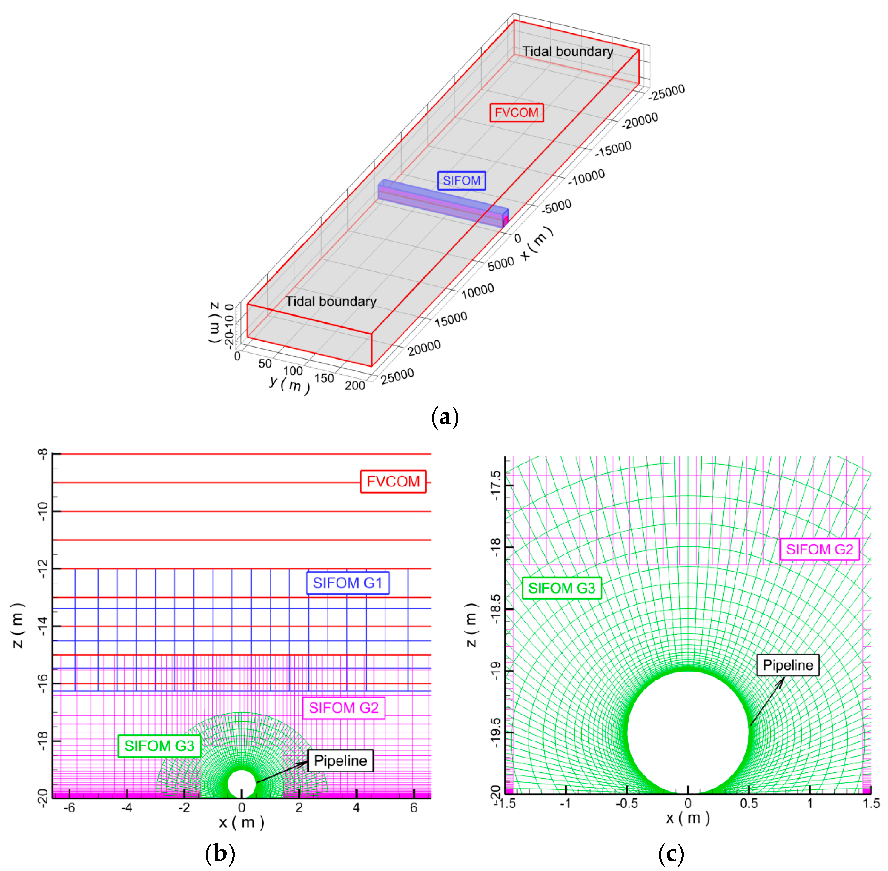
The influence factors include pipeline diameter, tide amplitude and water depth. The computational domain is 50 km in length, 200 m in width, with a pipeline laid on the seabed. The boundaries of the computational domain are controlled by the tidal elevation. The mesh of FVCOM covers the entire flow domain, and SIFOM contains three sets of grids, one (G3) of which wraps the pipeline, with the other two sets of grids (G1 and G2) enclosing the rest of the near-field region, as shown in Figure 9

The surface elevation at the boundaries of the flow domain is prescribed as Asin(kx − ωt), in which A is the amplitude of the tide, k the wave number, and ω the frequency. Considering the regular semi-diurnal tide, the period of the tide is set to be 12 h, which corresponds to astronomical tides.

The meshes include 1360 elements in the horizontal plane and 21 layers of grids in the vertical direction in the FVCOM. As for the SIFOM, the pipeline diameter has some effects on the mesh which closes to the pipeline (namely, grid G3 in Figure 9), because there is a fluid boundary layer around the pipeline. If the mesh is so rough that the boundary layer is ignored, the detailed flow characteristics around the pipeline are hard to be captured and the accuracy of the results may be lower by 20% to 40% than the actual results. In order to ensure the accuracy of the simulation, the Y-plus theory [32] is adopted when the mesh is set around the pipeline. When the pipeline diameter is 0.3 m, the layer thickness of mesh next to the pipeline is the minimum of 0.001 m which is also satisfied for the simulations of the larger pipelines. Then, the layer thickness of mesh increases from the first boundary layer of 0.001 m based on the increasing ratio of 1.12. It can not only ensure the calculation accuracy, but also reduce the number of grids resulting in the reduction of the computing time.

With the expansion of the calculation range in SIFOM, compared with the flow field, the pipeline is rather smaller and the effect of the pipeline on the whole field flow is weak. Besides, with the increase of the mesh layer based on the increasing ratio of 1.12, the effect of the pipeline diameter on the scale of grids also can be ignored in the far flow field. So, the lengths in x-direction of the grids (G1 and G2) are the similar in all cases in this section. In summary, the total number of grids in SIFOM is 39,996, with grid spacing refined as 0.001 m at the wall of the pipe and the seabed.

4.1.2. Effect of Pipeline Diameter

In this simulation, the influence of pipeline diameter on hydrodynamic forces acting on the pipeline is studied. The meshes and calculation settings are represented in the Section 4.1.1. The tidal amplitude A is 1 m and water depth H is 20 m. The pipeline diameter D is designed to 0.3 m, 0.7 m, 1.0 m, 1.3 m and 1.7 m, respectively.

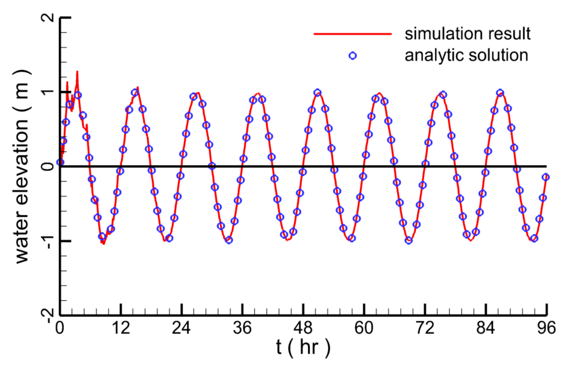
In the calculation domain, a gauge is set above the pipeline to monitor the free surface elevations, which indicates that the numerical result satisfies the analytical result well (Figure 10). Therefore, the target tide can be simulated accurately in the study.

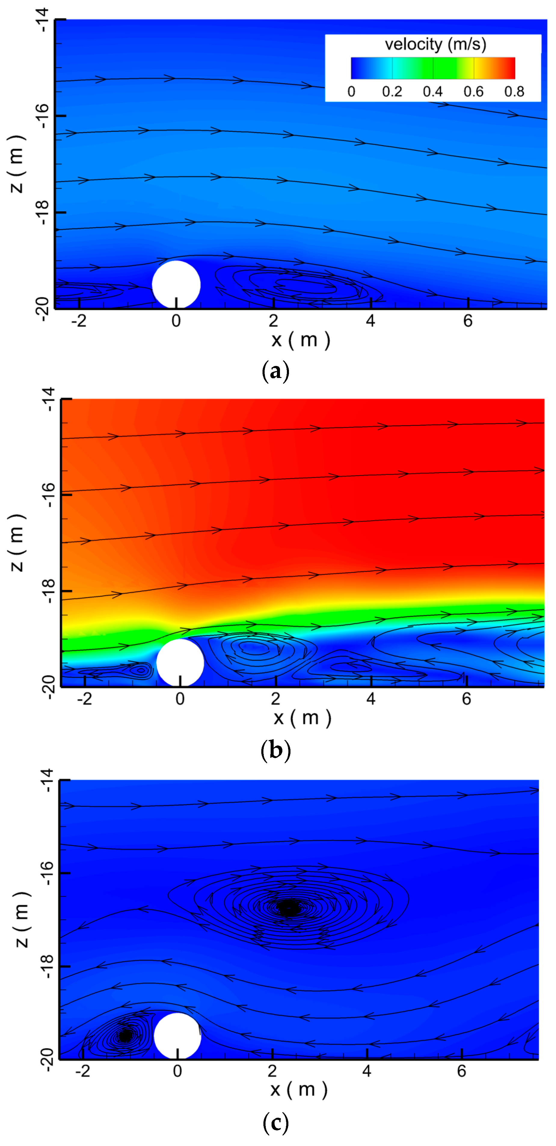
When the pipeline diameter is 1 m, the instantaneous flow structures at time instant t₁, t₂ and t₃ are depicted in Figure 11. At time t₁, the flow velocity of the whole flow field is quite low (Figure 10a) since the flood tide has just begun. It is seen that there is one vortex behind the pipeline at the beginning of the development of flow field. The length of vortex is about 4 m and the shape of the vortex is flat. The vortex under tidal flow is much more than that under the wave, because the vortex formation is subject to several influence factors that the period of the tide is very long and the velocity changes slowly. Correspondingly, the period of vortex shedding is also relatively long and the swirl evolves slowly. Meanwhile, the seabed also affects the formation of the whirlpool to some extent. Then, the tide flow moves towards the right gradually, leading to a number of vortices behind or at the right side of the pipe at time t₂ (Figure 11b). At this time, both the velocity of the flow field and the forces on the pipeline reach the maximum. When the tide has reversed its direction afterwards at time t₃, there are still some vortices at the left side of the pipe (Figure 11c). Interestingly, at this moment, the reversed current takes place underneath the top current, which remains flowing towards the right; while the middle and bottom layers of water move in opposite directions. The flow is very weak at this time and there is a larger whirlpool appearing at the intersection of the flow field.

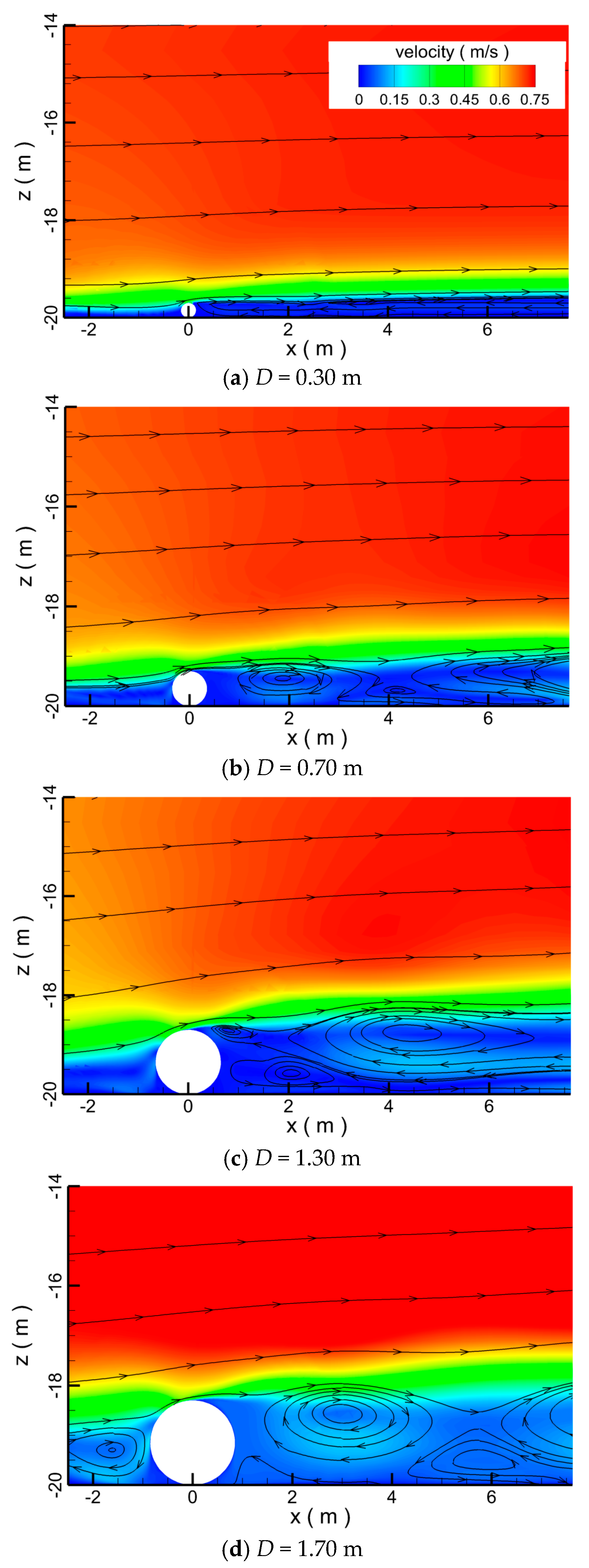
When the pipeline diameter changes and the tidal free surface elevation above the pipeline reaches the maximum, the flow fields are shown in Figure 12. With the increase of pipeline diameter, the velocity above the pipeline increases and the swirls behind the pipeline become bigger and bigger, while the vortices fall off the pipeline constantly with a flat and long shape.

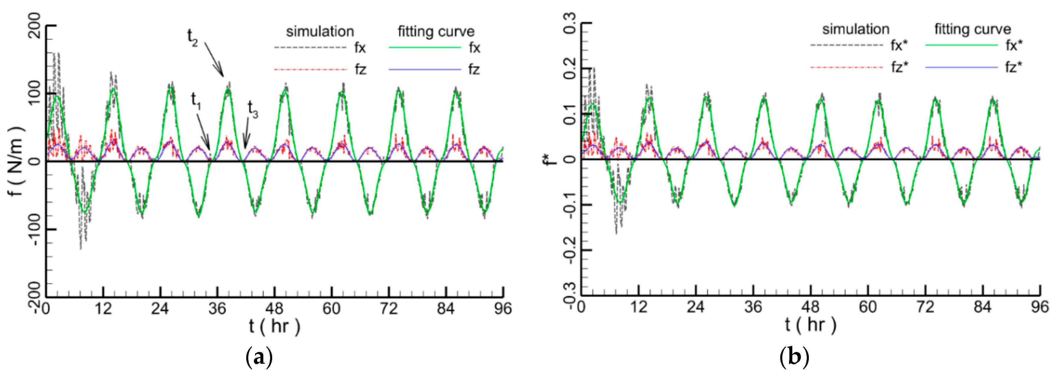
When the pipeline diameter is 1 m, the hydrodynamic forces on the pipeline are displayed in the Figure 13. The time instants t₁, t₂ and t₃ correspond to three moments of flow files in Figure 11a–c, respectively. The simulation time of tidal flow is four days, namely 96 h. f_x and f_z are the horizontal and vertical hydrodynamic forces on unit length of pipeline, respectively. The maximum horizontal and vertical hydrodynamic forces are 108.96 N/m and 29.42 N/m, respectively. The dotted line represents the simulation results of SIFOM–FVCOM, while the solid line is the filtering curve which is an average curve made with a filtering frequency of 0.30 Hz depending on the simulation results. There are two reasons for the addition of the filtering curve in every figure. Firstly, due to the turbulence of local flow around the pipeline, the simulation forces on the pipeline fluctuate to a certain extent in a short time. With the fluctuation of the tide, the forces on the pipeline also fluctuate regularly in a long time. In order to show the fluctuation regularity of the force in the long period, the smooth fitting filtering line is calculated. Secondly, due to the filtering curves are smooth and match the simulation results well, when the effects of different influence factors on the forces are analyzed, the filtering curves can be as the reference lines which can obviously demonstrate the force changes in different conditions. In order to compare the forces in the different cases conveniently, the predicted horizontal and vertical hydrodynamic forces are normalized with the hydrostatic force in this basic case. The formula of the hydrostatic force is written as: F_s = ρgHS where ρ is water density, g is the gravity, H is the water depth, S is the section area of the pipeline (S = πD²/4). (In the rest of the paper, the predicted hydrodynamic forces are also normalized using this force). The non-dimensional horizontal and vertical forces are represented by fx* and fz*. Due to the oscillatory flow of the tide, the forces on the pipeline change periodically and symmetrically with a period of 12 h. At the beginning of the simulation, the unstable flow causes the force to fluctuate severely. When the flow field becomes stable after about 20 h, the change of force tends to become gentle gradually. However, because of the turbulence of flow, there is still little fluctuation of forces. Furthermore, the hydrodynamic forces on the pipeline at the flood tide are larger than that at the ebb tide. Because in the process of tide propagation, the higher the tidal elevates, the larger the bottom horizontal velocity grows. The difference of velocity leads to the change of the hydrodynamic forces. From the figure, it is seen that the horizontal force has two peaks that are about the same in magnitude but opposite in direction, while the vertical force is always in the upward direction. The peak values in the horizontal and vertical directions occur at the same time.

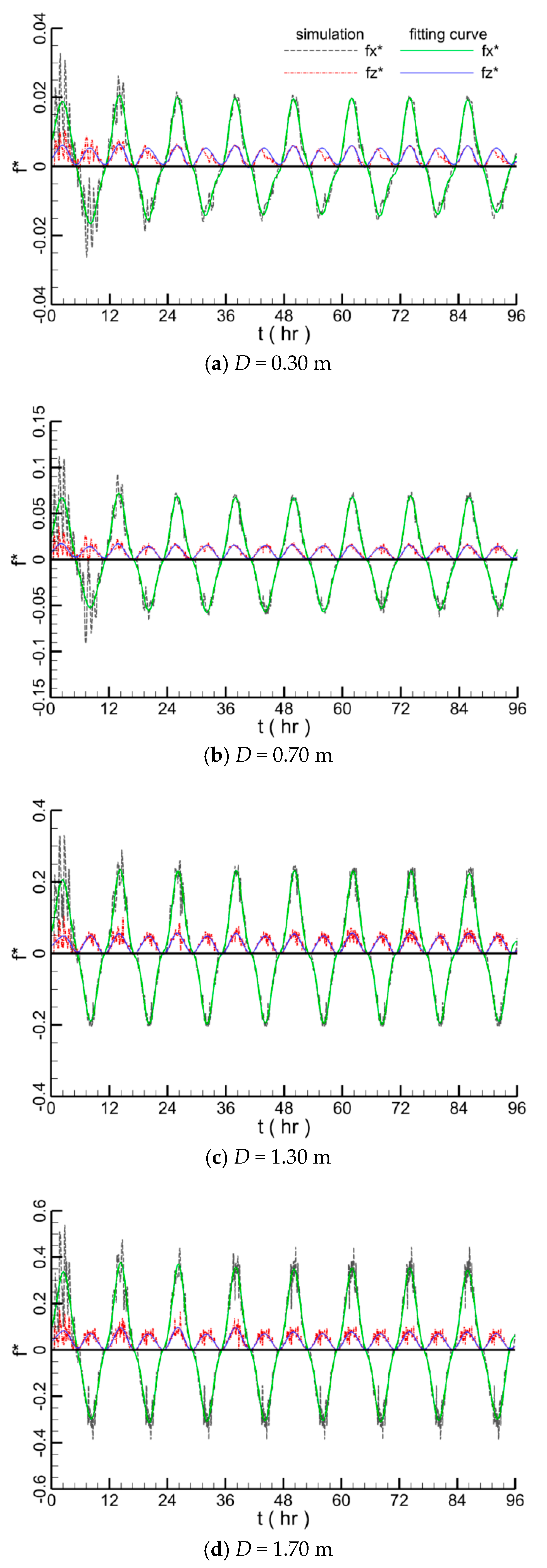
The simulation results and filtering curve of hydrodynamic forces with different pipeline diameters are shown in Figure 14. All the hydrodynamic forces on the submarine pipeline oscillate intensely at the beginning of simulation due to the unsteady tidal flow. When the tidal flow becomes stable, with the increase of pipeline diameter, the projection area in the force direction also enlarges, leading to a larger force on the pipeline.

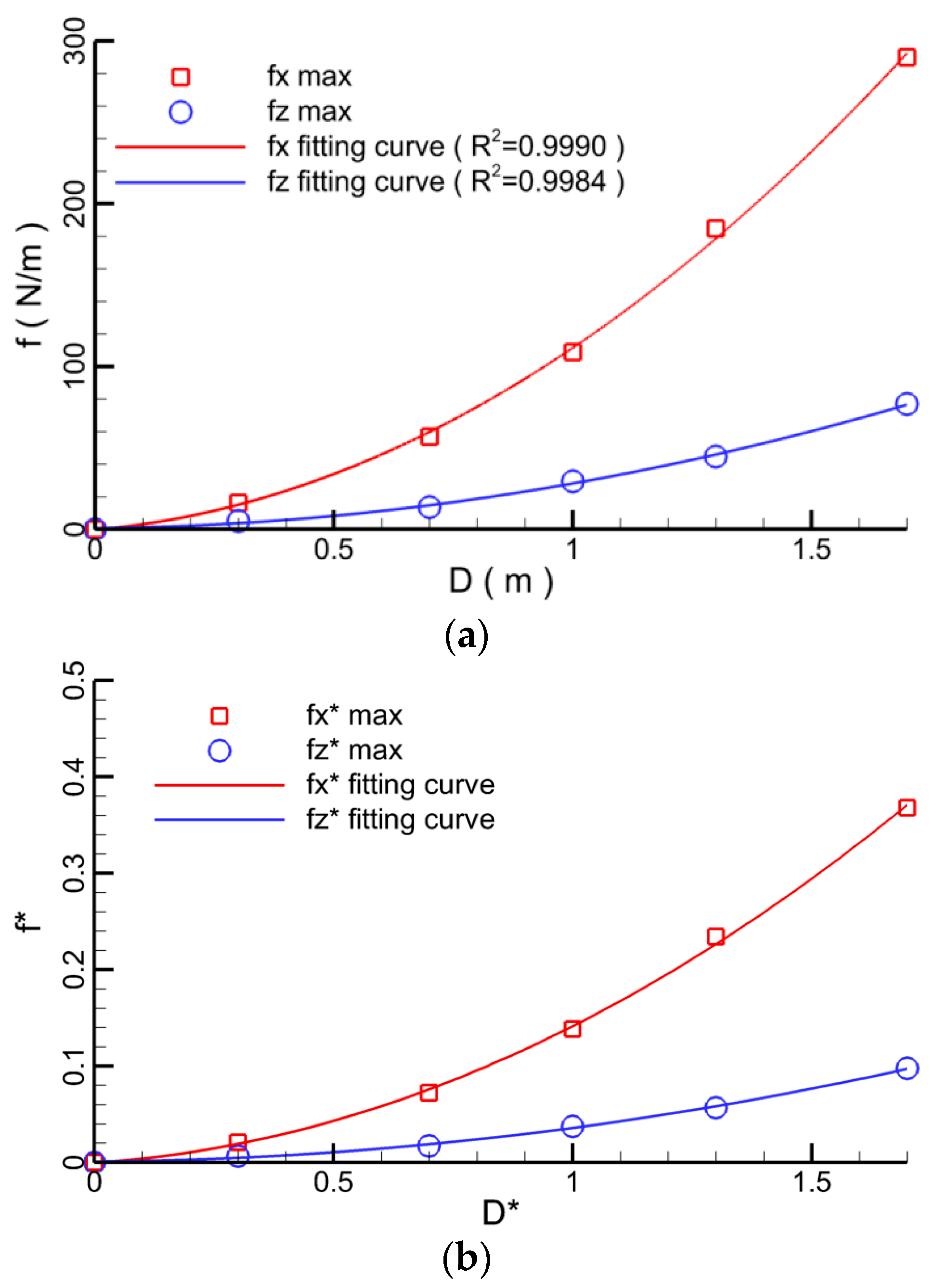
Depending on the simulation results, the maximum force values at different pipelines are drawn in Figure 15, where the red and blue lines are the fitting curves. It can be seen more clearly that the maximum force value increases as the pipe diameter increases.

4.1.3. Effect of Tidal Amplitude

In this section, the influence of tidal amplitude on the hydrodynamic forces acting on the pipeline is analyzed. The meshes and calculation settings are represented in the Section 4.1.1. The pipeline diameter D is 1 m and water depth H is 20 m. The tidal amplitude is set to 0.25 m, 0.5 m, 1.0 m, 1.5 m and 2.5 m, respectively.

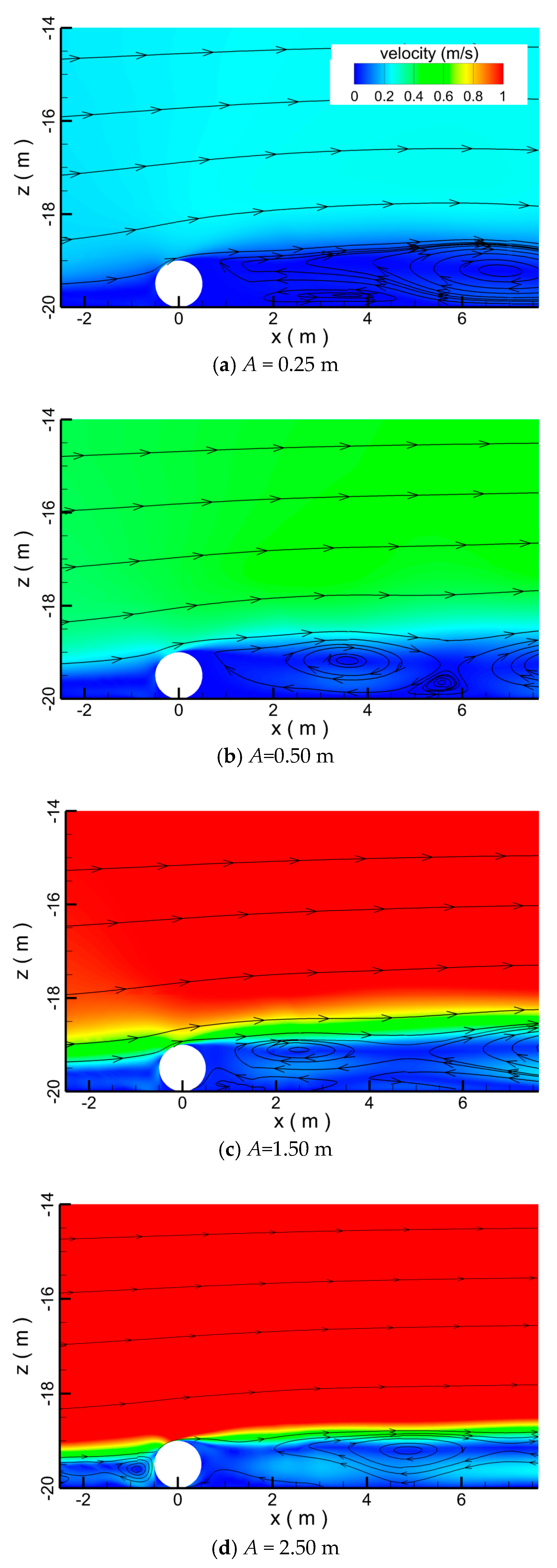
Figure 16 shows the flow fields around the pipeline when the crest of the tide is at the top of the pipeline. When the tidal amplitude is 0.25 m, the maximum velocity around the pipeline is 0.35 m/s. As the tidal amplitude reaches 2.5 m, the maximum velocity around the pipeline increases to about 1 m/s. The higher the tidal water elevation is, the larger the velocity grows. Additionally, there are whirlpools formed and shed behind the pipeline at all flow velocities.

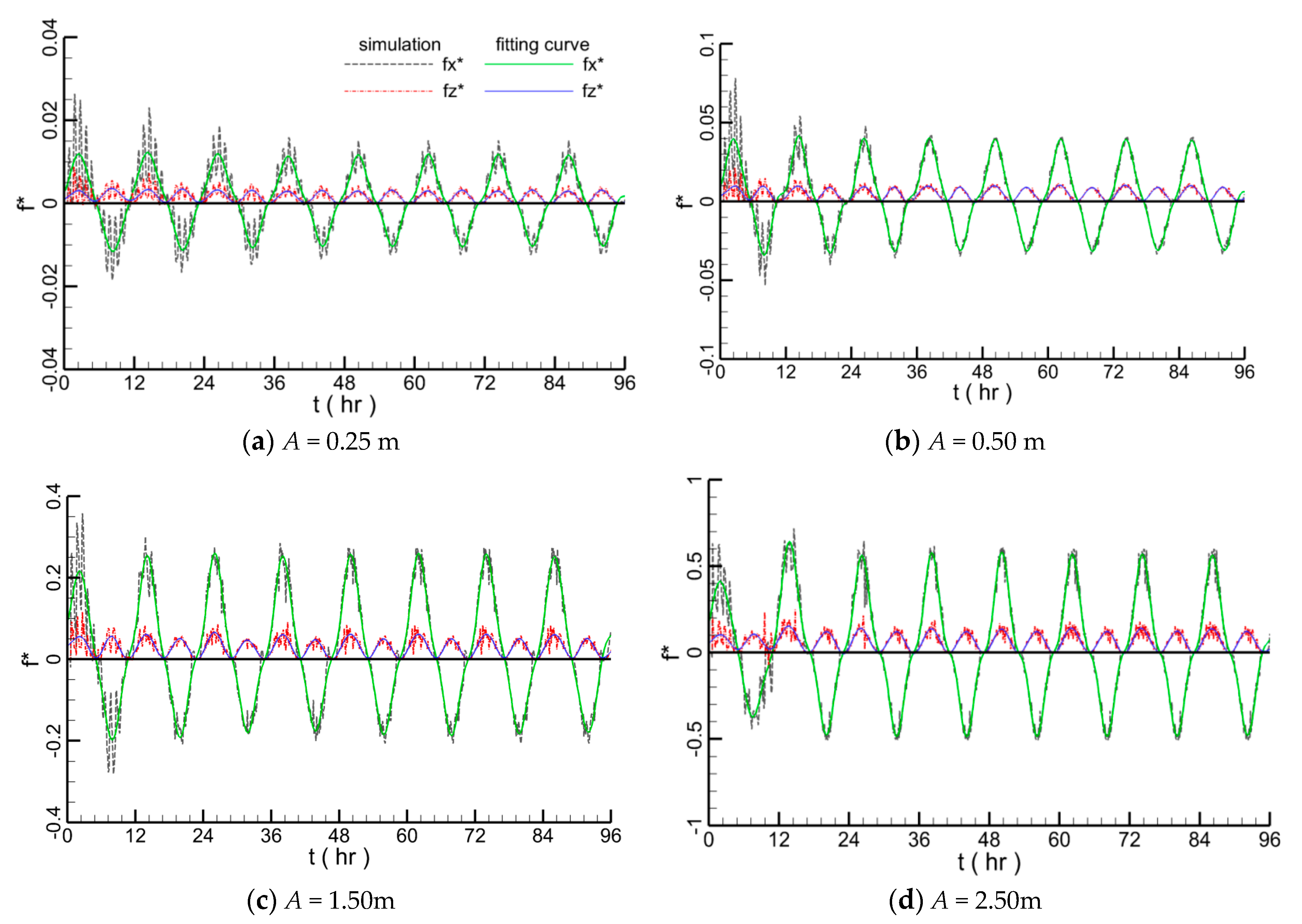
The simulation results of hydrodynamic forces are depicted in Figure 17. It is seen that the oscillation of force curves is severer with the tidal amplitude of 0.25 m than that of other curves because larger tidal amplitude leads to larger velocity around the pipeline, thus a larger force. When the hydrodynamic forces are more than the forces caused by flow turbulence, the influence of turbulence on the pipeline appears weak. In addition, the performance of the hydrodynamic forces on the pipeline is more obvious with the increase of tidal amplitude.

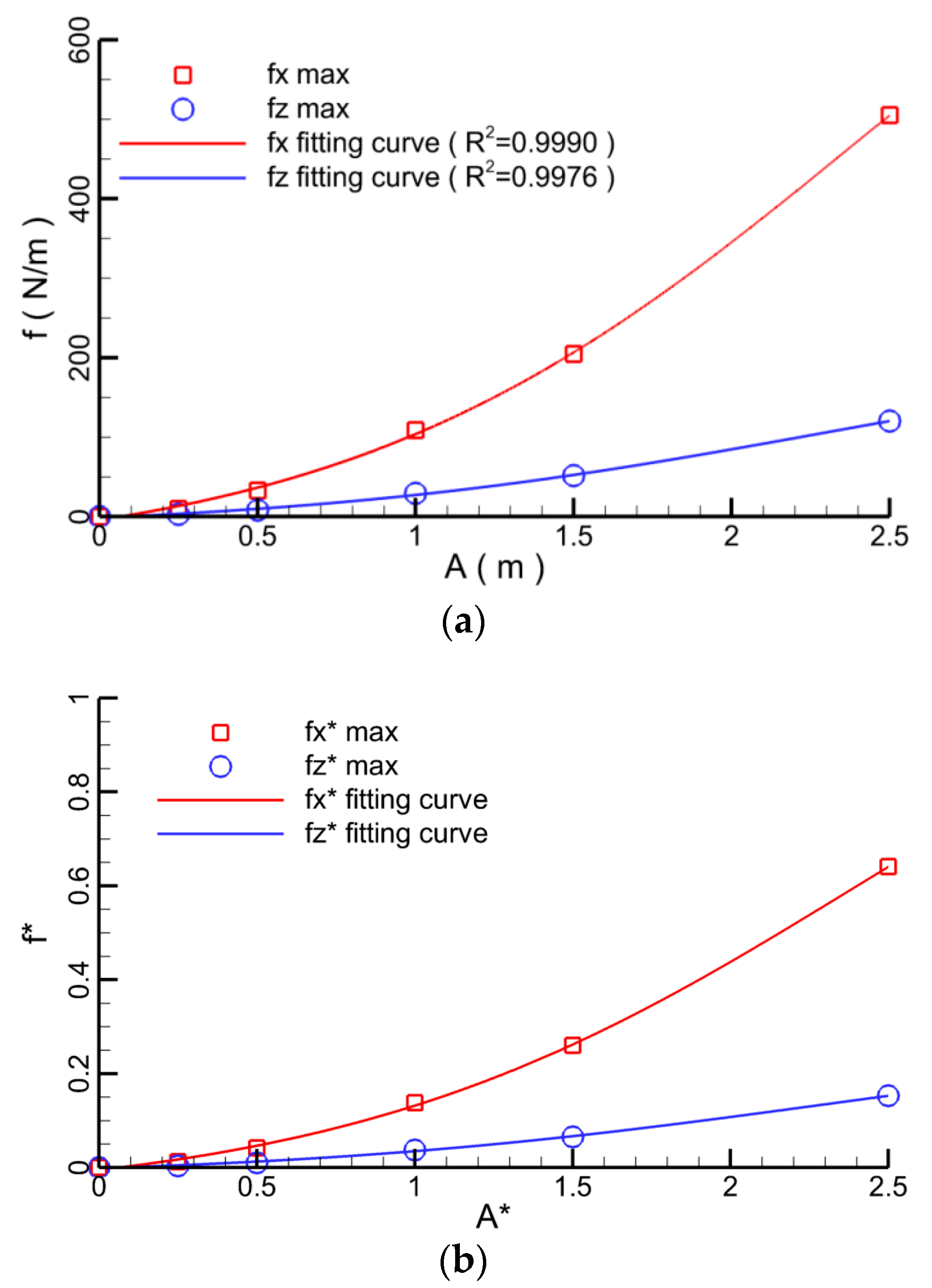
In Figure 18, the maximum force values at different tidal amplitudes are displayed. As the tidal amplitude changes from 0.5 m to 1.5 m, the slope of the fitting curve reaches the largest and the increase rate of the pipeline force reaches its fastest level.

4.1.4. Effect of Water Depth

In this section, the influence of water depth on the hydrodynamic forces acting on the pipeline is researched. The meshes and calculation settings are represented in Section 4.1.1. The tidal amplitude A is 1.0 m and pipeline diameter D is 1.0 m. The water depth H is designed to be 10 m, 15 m, 20 m, 30 m and 50 m, respectively.

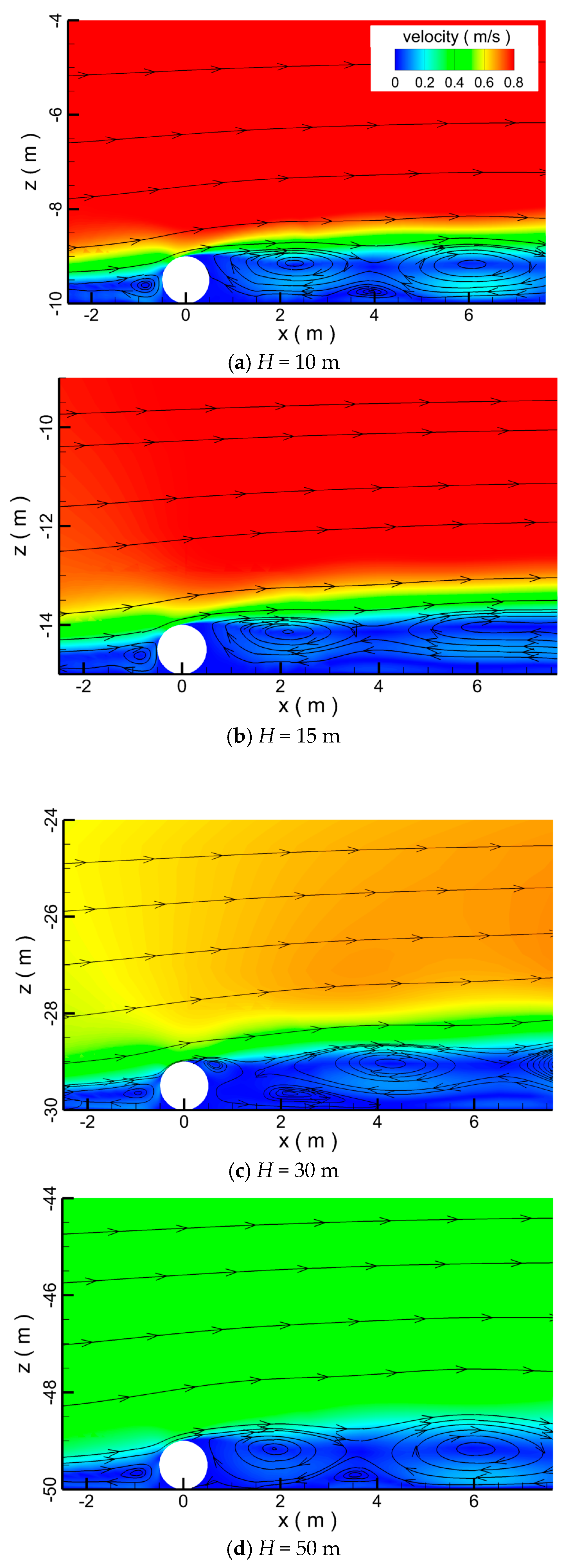
As can be seen in Figure 19, with the increase of water depth, the velocity of the flow field around the pipeline decreases. Due to the obstruction of the pipeline, the backflow in the front of the pipeline leads to the formation of the whirlpool, and there are also some vortexes behind the pipeline.

The simulation results of hydrodynamic forces on the submarine pipeline at different water depth are displayed in Figure 20. Due to the turbulence around the pipeline, the simulation curve of force is not smooth. With the increase of water depth, the hydrodynamic forces on the submarine pipeline continue to decrease; however, the static pressure on the pipeline increases. Therefore, for pipelines laid on the deep sea, static pressure is the main factor which leads to damage of the pipelines.

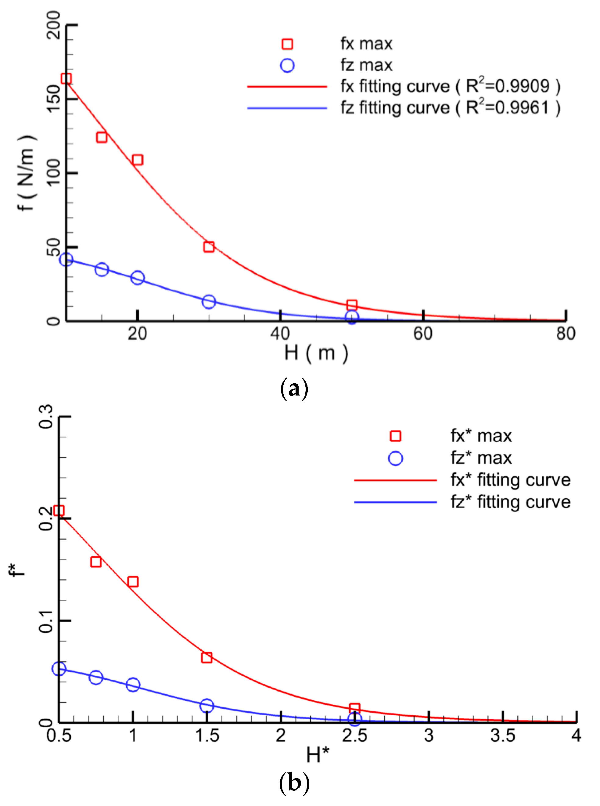
The maximum values of hydrodynamic forces at different water depth are shown in Figure 21. As can be seen, the influence of the water depth on the hydrodynamic forces is quite weak for cases of water depth exceeding 25 m.

4.1.5. Hydrodynamic Forces on the Submarine Pipeline

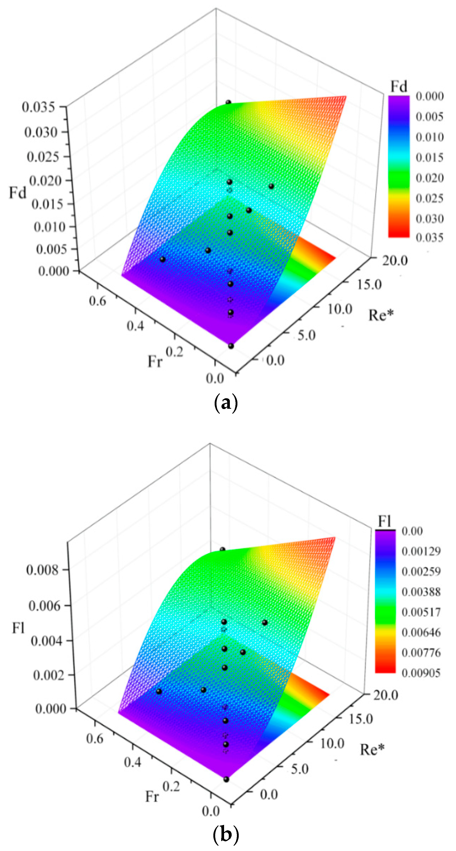
The computed hydrodynamic forces on the pipe consist of the pressure and the shear stress, which are affected by the flow characteristics. All the influence factors (pipeline diameter, tidal amplitude and water depth) induce the change of flow characteristics which can be reflected by the characteristic coefficients of Froude number and Reynolds number. For example, Reynolds number can be used to distinguish the laminar and turbulent flow. Besides, the hydrodynamic forces are also related to the characteristic coefficients, for instance, the resistance of the body in flow can be characterized by Reynolds number and the relative magnitude of inertia force to the gravity can be characterized by Froude number. So, the maximum hydrodynamic forces are considered to be a function of the Froude and Reynolds numbers. Depending on the method of the polynomial fitting and the discrete data of the maximum forces in previous research, the two fitting curves are determined. The maximum horizontal and vertical forces (F_x,max and F_z,max) in every case are normalized by F_D = F_x,max/(ρgDA) and F_L = F_z,max/(ρgDA), respectively. In order to eliminate the effect of the constant value of the kinematic viscosity coefficient on the empirical coefficients of the formulas, the Reynolds number is redefined by the Re* = Re|ν|, where |ν| is the value of the kinematic viscosity coefficient. The formulas for the maximums of hydrodynamic forces are written as:

$$F_D=-3.88\times {10}^{-2}{\mathrm{Re}}^{*2}Fr+1.11\times {10}^{-2}{\mathrm{Re}}^{*2}+5.39\times {10}^{-2}{\mathrm{Re}}^{*}Fr$$

(12)

$$F_L=-1.07\times {10}^{-2}{\mathrm{Re}}^{*2}Fr+2.9\times {10}^{-3}{\mathrm{Re}}^{*2}+1.45\times {10}^{-2}{\mathrm{Re}}^{*}Fr$$

(13)

The regression statistics index numbers R² of F_D and F_L are 0.881 and 0.860, respectively. The Froude number and Reynolds number are calculated based on the water depth H, pipe diameter D, and velocity v*. The velocity is evaluated by v* = A(g/H)^1/2. The modeling results and the extracted formulas are plotted in Figure 22.

4.2. Hydrodynamics around Submarine Pipeline with Scour

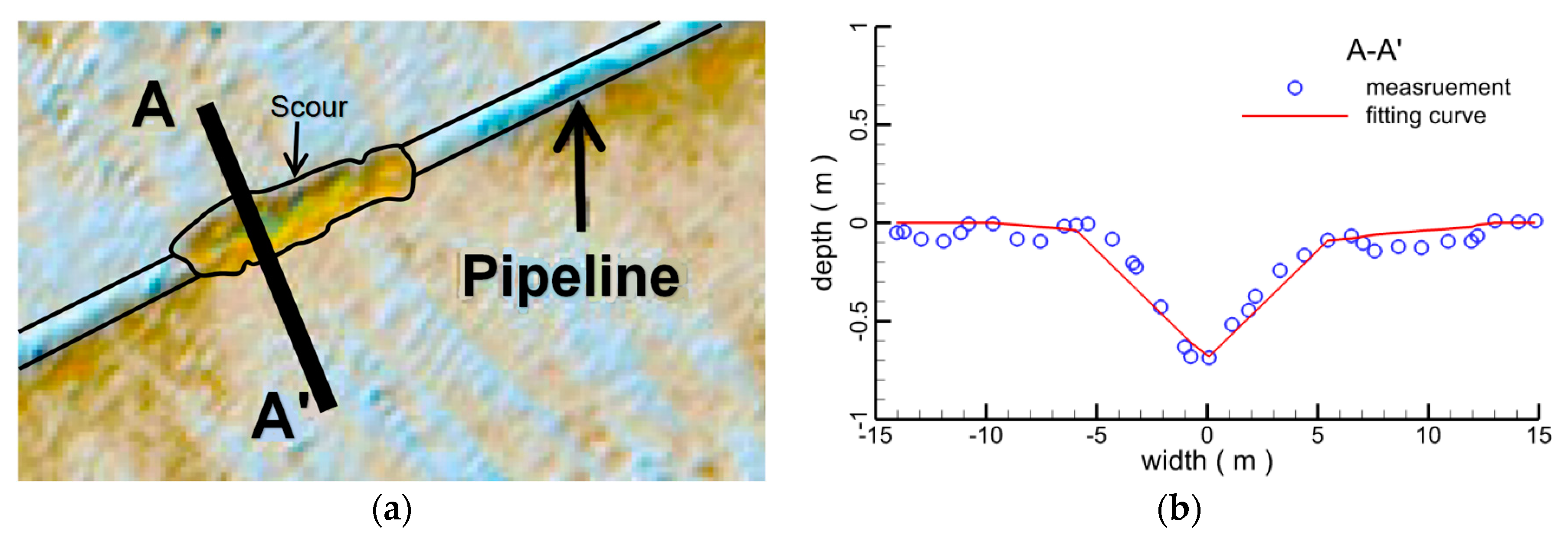
Due to the influence of flows on the sediment of seabed, the scour around the pipeline on the seabed occurs easily which may induce suspension of the pipeline. The Figure 23a shows the scour morphology around the DF1-1 submarine pipeline which lies off the west coast of Dongfang, Hainan Island. The data of scour hole in Figure 23b are measured using a dual-frequency side-scan sonar and a swath sounder system [27].

Depending on the measurement, the formula of fitting curve of scour hole is evaluated as:

$$z=\{\begin{array}{c}0.11\left|x\right|-h\\ 0\end{array}\begin{array}{c}\\ \end{array}\begin{array}{c}0.11\left|x\right|\le h\\ 0.11\left|x\right|>h\end{array}$$

(14)

in which the deepest point of the scour hole is defined as the original point, namely x = 0; h is the depth of the scour hole.

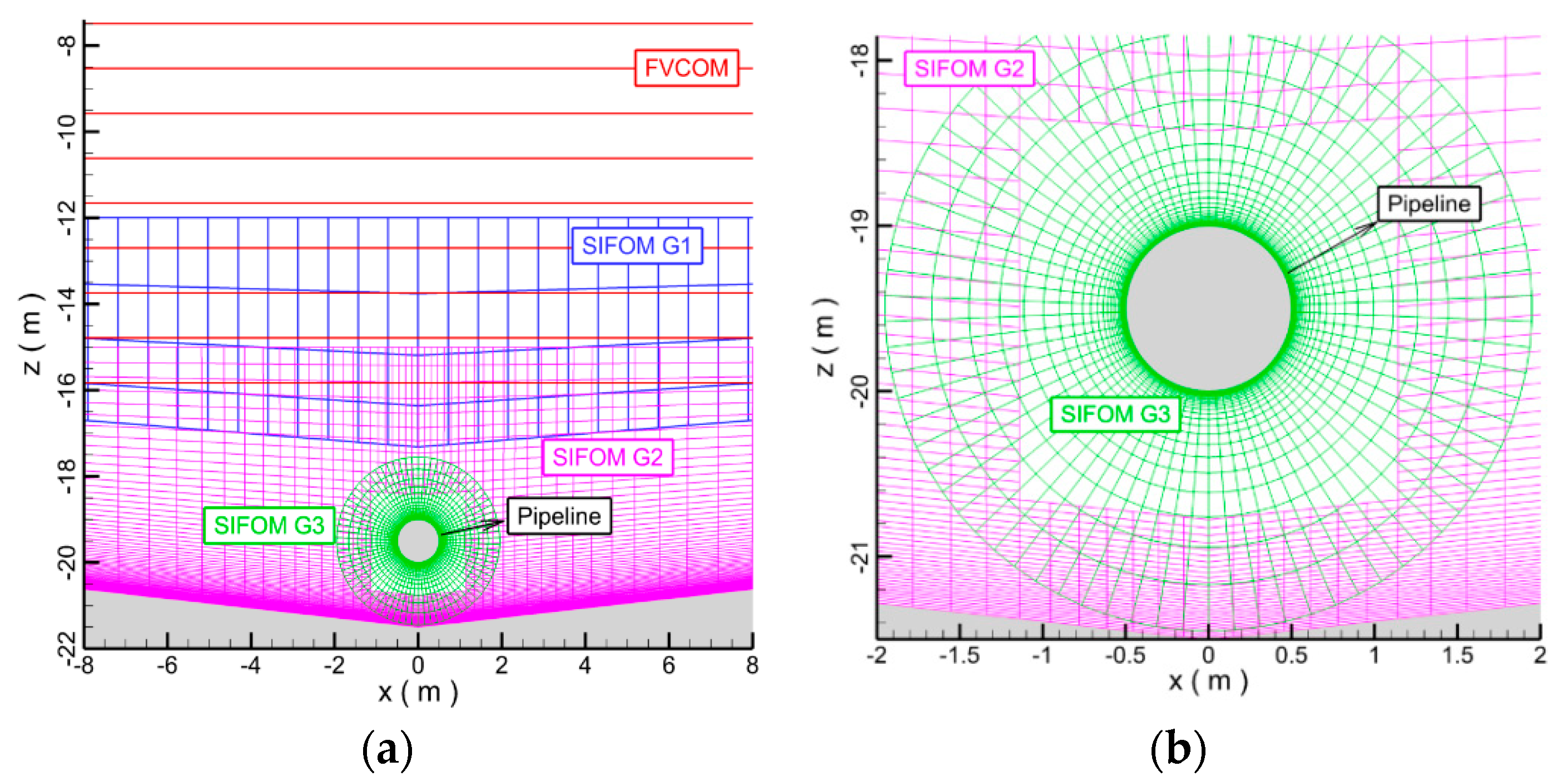
In this section, three different cases are simulated and analyzed. Based on the fitting Equation (14) of scour hole, the scour hole of simulation model is established. The depth of scour hole is 0.25 m, 0.875 m and 1.5 m, respectively, and the width of the scour hole is 4.56 m, 15.91 m and 27.27 m, respectively. The water depth is 20 m. The tidal wave amplitude is 1 m and the pipeline diameter is 1 m. The coordinate of the pipeline center is (x, z) = (0 m, 0.5 m). The pipeline is taken as a rigid body and the scour hole maintains a steadily evolving topography. In the model, there are three structure grids (G1, G2 and G3) of SIFOM and one unstructured grid of FVCOM. The meshes of SIFOM–FVCOM are shown in the Figure 24, in which the pipeline is constructed by O-mesh (G3) and the mesh of FVCOM is similar to that in Section 4.1. The resolution of mesh closing to the pipeline and seabed is 0.001 m.

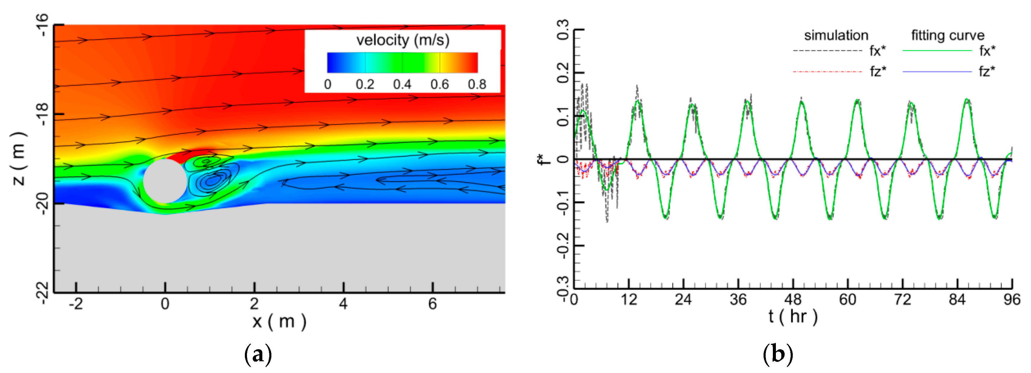
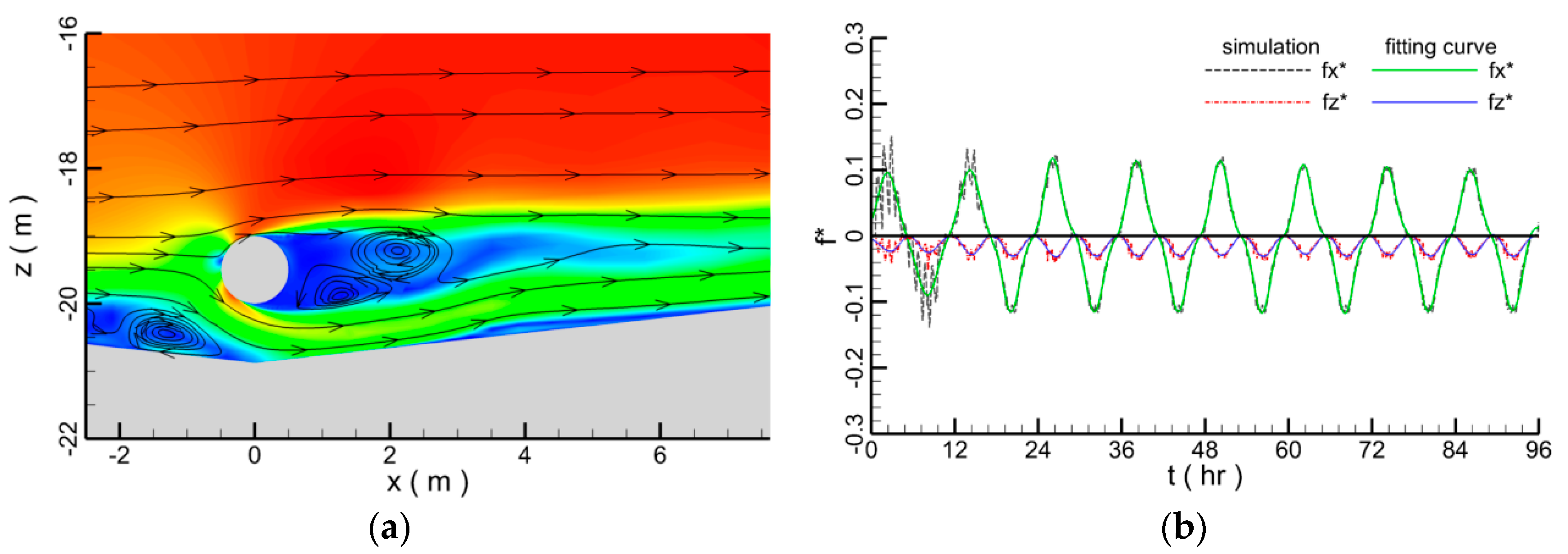
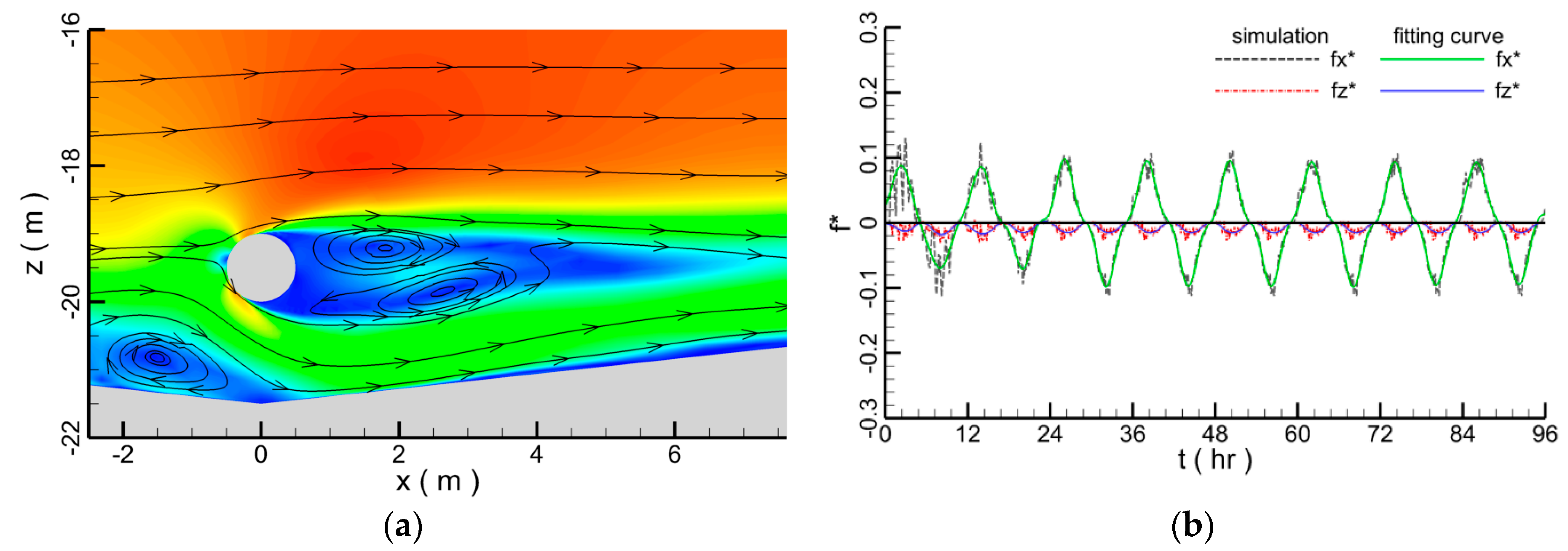
When the wave crest of tide is at the top of the pipeline, the velocity of flow field reaches the maximum and the flow fields are shown in Figure 25a, Figure 26a and Figure 27a. The flow velocity above the pipeline decreases with the increase of the scour depth, since when the depth of scour hole increases, more water passes the scour hole below the pipeline which induces the volume of water above the pipeline to decrease. Besides, vortex shedding can be found behind the pipeline in every case. In Figure 26a and Figure 27a, it is seen that the backflow leads to the formation of whirlpools at the upward slope of scour hole as a result of the obstruction of the pipeline.

Under the effect of the tidal flow, hydrodynamic forces on the pipeline change cyclically (Figure 25b, Figure 26b and Figure 27b). The vertical forces stay negative since the average velocity above the pipeline is smaller than that under the pipeline, while the vertical downward force on the pipeline greater than the upward force according to the Bernoulli equation.

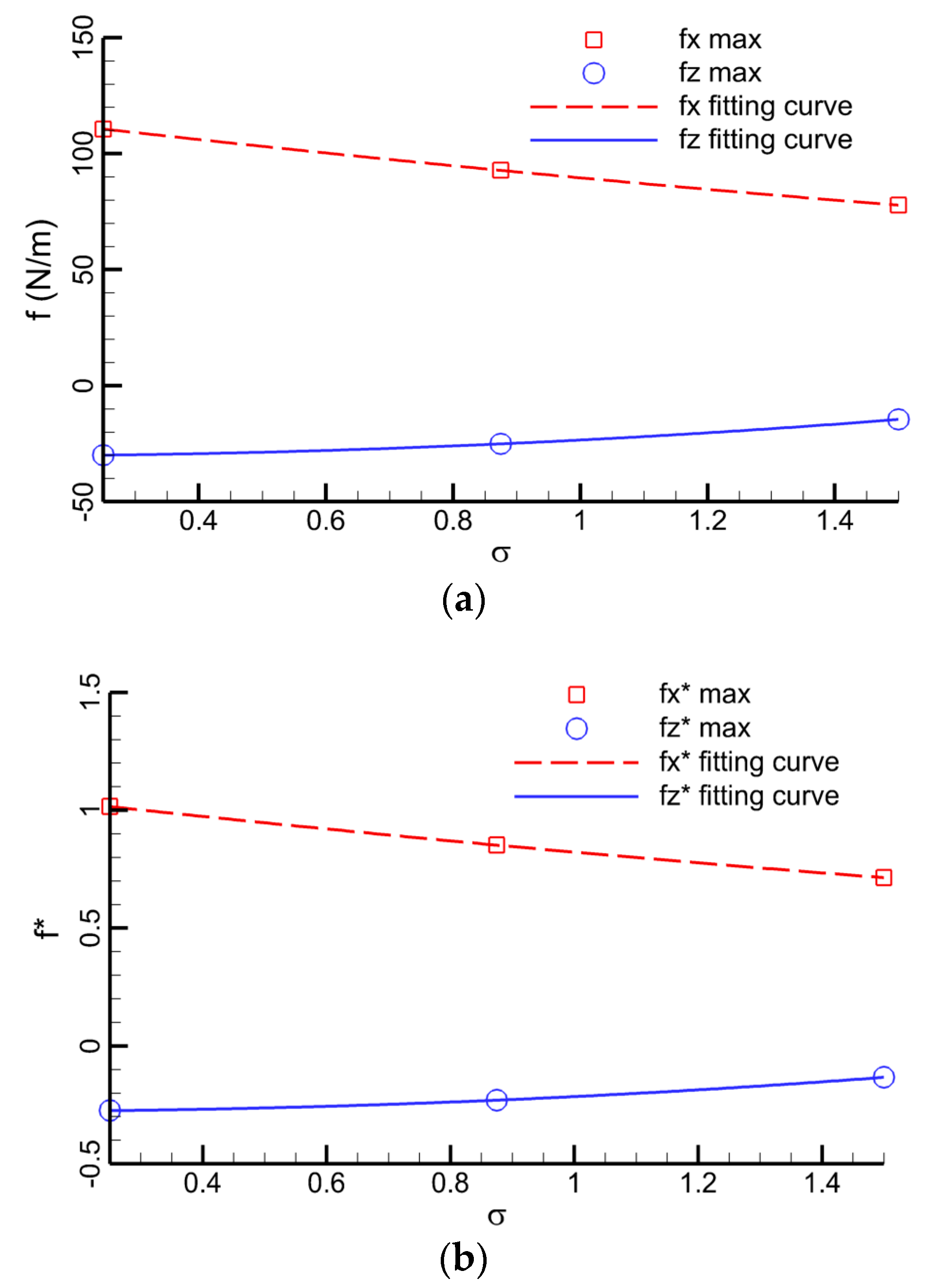
With the increase of scour depth, the maximum horizontal hydrodynamic forces reduce and the vertical hydrodynamic forces grow. The trend of hydrodynamic forces at different scour depths is illustrated in Figure 28.

5. Conclusions

Using the SIFOM–FVCOM system, a modeling study is carried out on hydrodynamics at submarine pipelines under the force of tidal currents. The main conclusions are summarized below. Through the comparison between the numerical results and experimental measurements, the simulation accuracy of SIFOM–FVCOM modeling is verified. Depending on this modeling, the influence of pipeline diameter, tidal amplitude and water depth on the hydrodynamic forces acting on the pipeline is investigated. It is concluded that with the increase of pipeline diameter and tidal amplitude, the hydrodynamic forces on the pipeline increase. However, the hydrodynamic force decreases with the water depth increasing. Besides, flow structures around the pipelines are also revealed under different conditions. Since the period of tide is very long and the velocity changes slowly, the falling vortex behind the pipeline appears flat and long, while the period of vortex shedding is relatively long and the swirl evolves slowly as well. In the meantime, the seabed also affects the formation of the whirlpool to some extent. Furthermore, the maximum corresponding hydrodynamic forces on the pipeline are empirically formulated as a function of the Froude and Reynolds numbers. According to the real cases in the submarine pipeline engineering, the hydrodynamics around the suspended submarine pipeline is researched. When the seabed scour appears around the pipeline, the pipeline is in the suspended state. The results show that with the increase of scour depth, the hydrodynamic forces on the submarine pipeline decrease.

This paper demonstrates the capability of the SIFOM–FVCOM system in direct numerical simulations of high-fidelity multi-physics phenomena at vastly distinct scales, which is more advantageous than existing models in some extent. The results presented in this paper might be useful and advisable in the mechanism of the flows and the research of pipeline in the real marine environment from an engineering point of view.

References

- Shankar, N.J.; Cheong, H.F.; Subbiah, K. Forces on a smooth submarine pipeline in random waves—A comparative-study. Coast. Eng. 1987, 11, 189–218. [Google Scholar] [CrossRef]
- Al-Dakkan, K.; Alsaif, K. On the design of a suspension system for oil and gas transporting pipelines below ocean surface. Arab. J. Sci. Eng. 2012, 37, 2017–2033. [Google Scholar] [CrossRef]
- Kok, N.J. Lift and Drag Forces on a Submarine Pipeline in Steady Flow. Ph.D. Thesis, University of Cape Town, Cape Town, South Africa, 1988. [Google Scholar]
- Li, X.; Li, M.G.; Zhou, J. Experimental study of the hydrodynamic force on a pipeline subjected to vertical seabed movement. Ocean Eng. 2013, 72, 66–76. [Google Scholar] [CrossRef]
- Yang, B.; Gao, F.P.; Wu, Y.X.; Li, D.H. Experimental study on vortex-induced vibrations of submarine pipeline near seabed boundary in ocean currents. China Ocean Eng. 2006, 20, 113–121. [Google Scholar]
- Mattioli, M.; Alsina, J.M.; Mancinelli, A.; Miozzi, M.; Brocchini, M. Experimental investigation of the nearbed dynamics around a submarine pipeline laying on different types of seabed: The interaction between turbulent structures and particles. Adv. Water Res. 2012, 48, 31–46. [Google Scholar] [CrossRef]
- Mattioli, M.; Mancinelli, A.; Brocchini, M. Experimental investigation of the wave-induced flow around a surface-touching cylinder. J. Fluid Struct. 2013, 37, 62–87. [Google Scholar] [CrossRef]
- Pierro, A.; Tinti, E.; Lenci, S.; Brocchini, M.; Colicchio, G. Investigation of the dynamic loads on a vertically-oscillating circular cylinder close to the sea bed: The role of viscosity. J. Offshore Mech. Arct. Eng. 2017, 139, 061101. [Google Scholar] [CrossRef]
- Ong, M.C.; Utnes, T.; Holmedal, L.E.; Myrhaug, D.; Pettersen, B. Numerical simulation of flow around a smooth circular cylinder at very high Reynolds numbers. Mar. Struct. 2009, 22, 142–153. [Google Scholar] [CrossRef]
- Cheng, L.; Chew, L.W. Modelling of flow around a near-bed pipeline with a spoiler. Ocean. Eng. 2003, 30, 1595–1611. [Google Scholar] [CrossRef]
- Chiew, Y.M. Mechanics of local scour around submarine pipelines. J. Hydraul. Eng. 1990, 116, 515–529. [Google Scholar] [CrossRef]
- Brors, B. Numerical modeling of flow and scour at pipelines. J. Hydraul. Eng. 1999, 125, 511–523. [Google Scholar] [CrossRef]
- Sumer, B.M.; Fredsoe, J. Wave scour around a large vertical circular cylinder. J. Waterw. Port Coast. Ocean Eng. 2001, 127, 125–134. [Google Scholar] [CrossRef]
- Myrhaug, D.; Ong, M.C.; Føien, H.; Gjengedal, C.; Leira, B.J. Scour below pipelines and around vertical piles due to second-order random waves plus a current. Ocean Eng. 2009, 36, 605–616. [Google Scholar] [CrossRef]
- Zhou, X.L.; Wang, J.H.; Zhang, J.; Jeng, D.S. Wave and current induced seabed response around a submarine pipeline in an anisotropic seabed. Ocean Eng. 2014, 75, 112–127. [Google Scholar] [CrossRef]
- Postacchini, M.; Brocchini, M. Scour depth under pipelines placed on weakly cohesive soils. Appl. Ocean Res. 2015, 52, 73–79. [Google Scholar] [CrossRef]
- Zhao, M.; Vaidya, S.; Zhang, Q.; Cheng, L. Local scour around two pipelines in tandem in steady current. Coast. Eng. 2015, 98, 1–15. [Google Scholar] [CrossRef]
- Lam, K.Y.; Wang, Q.X.; Zong, Z.A. Nonlinear fluid-structure interaction analysis of a near-bed submarine pipeline in a current. J. Fluid Struct. 2002, 16, 1177–1191. [Google Scholar] [CrossRef]
- Lin, Z.B.; Guo, Y.K.; Jeng, D.S.; Liao, C.C.; Rey, N. An integrated numerical model for wave-soil-pipeline interactions. Coast. Eng. 2016, 108, 25–35. [Google Scholar] [CrossRef]
- Zhao, E.J.; Shi, B.; Qu, K.; Dong, W.B.; Zhang, J. Experimental and Numerical Investigation of Local Scour around Submarine Piggyback Pipeline under Steady Currents. J. Ocean Univ. China 2018, 17, 244–256. [Google Scholar] [CrossRef]
- Sabag, S.R.; Edge, B.L.; Soedigdo, I. Wake II model for hydrodynamic forces on marine pipelines including waves and currents. Ocean Eng. 2000, 27, 1295–1319. [Google Scholar] [CrossRef]
- Fringer, O.B.; Gerritsen, M.; Street, R.L. An unstructured-grid, finite-volume, nonhydrostatic, parallel coastal ocean simulator. Ocean Model. 2006, 14, 139–173. [Google Scholar] [CrossRef]
- Tang, H.S.; Qu, K.; Wu, X.G. An overset grid method for integration of fully 3D fluid dynamics and geophysics fluid dynamics models to simulate multiphysics coastal ocean flows. J. Comput. Phys. 2014, 273, 548–571. [Google Scholar] [CrossRef]
- Leonard, B.P. A stable and accurate convective modelling procedure based on quadratic upstream interpolation. Comput. Methods Appl. Mech. Eng. 1979, 19, 59–98. [Google Scholar] [CrossRef]
- Tang, H.S.; Keen, T.R.; Khanbilvardi, R. A model-coupling framework for nearshore waves, currents, sediment transport, and seabed morphology. Commun. Nonlinear Sci. Numer. Simul. 2009, 14, 2935–2947. [Google Scholar] [CrossRef] [Green Version]
- Chen, C.S.; Liu, H.D.; Beardsley, R.C. An unstructured, finite-volume, three-dimensional, primitive equation ocean model: Application to coastal ocean and estuaries. J. Atmos. Ocean. Technol. 2003, 20, 159–186. [Google Scholar] [CrossRef]
- Xu, J.S.; Pu, J.J.; Li, G.X. Field Observations of Seabed Scours around a Submarine Pipeline on Cohesive Bed. In Advances in Computational Environment Science; Lee, G., Ed.; Springer: Berlin, Germany, 2012; Volume 142, pp. 23–33. [Google Scholar]
- Jensen, B.L. Large-scale vortices in the wake of a cylinder placed near a wall. In Proceedings of the 2nd International Conference on Laser Anemometry-Advances and Applications, Strathclyde, UK, 21–23 September 1987; pp. 153–163. [Google Scholar]
- Liang, D.F.; Cheng, L. Numerical modeling of flow and scour below a pipeline in currents. Part I. Flow simulation. Coast. Eng. 2005, 52, 25–42. [Google Scholar] [CrossRef]
- Lyn, D.; Rodi, W. The flapping shear layer formed by flow separation from the forward corner of a square cylinder. J. Fluid Mech. 1994, 267, 353–376. [Google Scholar] [CrossRef]
- Catalano, P.; Wang, M.; Iaccarino, G.; Moin, P. Numerical simulation of the flow around a circular cylinder at high Reynolds number. Int. J. Heat Fluid Flow 2003, 24, 463–469. [Google Scholar] [CrossRef]
- White, F.M. Fluid Mechanics, 7th ed.; McGraw Hill Press: New York, NY, USA, 2009. [Google Scholar]
Figure 1.
Illustration of the orthogonal Cartesian coordinate system.
Figure 2.
The decomposition domains of Solver for Incompressible Flow on the Overset Meshes–Finite Volume Coastal Ocean Model (SIFOM–FVCOM) modeling around the submarine pipeline.
Figure 3.
The calculation meshes. (a) The horizontal plane mesh at z = −0.513 m. (b) The vertical plane mesh.
Figure 4.
Simulation of the flow passing a cylinder. (a) Computed flow field near the cylinder. (b) Comparison of the horizontal velocity distribution. (c) Comparison of the vertical velocity distribution. Circle-measurement [28], green dash line, modeling with ĸ-ε turbulence closure [29], blue solid line, SIFOM, red dash-dot line, SIFOM–FVCOM.
Figure 5.
Flow passes a cubic cylinder at bottom of channel. (a) Computed flow field near the square cylinder. (b) Comparison of the velocity distribution. Circle-Measurement [30], dash-dot line, DNS modeling, solid line, SIFOM–FVCOM.
Figure 6.
Flow field. (a) Velocity. (b) Vorticity.
Figure 7.
Comparison between simulation results and measurement data. (a) Mean pressure distribution. (b) Skin friction distribution.
Figure 8.
The numerical experimental sketch of flow passing a submarine pipeline.
Figure 9.
The model setup. (a) Computational domain. (b) Grids. (c) The mesh closing to pipeline.
Figure 10.
The free surface elevation comparison between numerical result and analytical solution.
Figure 11.
Simulated 2D flow field at the pipe. The flow in (a–c) are in order of time t1, t2 and t3.
Figure 12.
The flow fields around different diameter pipelines in time of t = 39 h.
Figure 13.
The hydrodynamic force of submarine pipeline. (a) Maximum force. (b) Non-dimensional maximum force.
Figure 14.
The hydrodynamic forces on the pipeline with different pipeline diameters.
Figure 15.
The maximum hydrodynamic forces at different pipelines. (a) Maximum force. (b) Non-dimensional maximum force.
Figure 16.
The flow fields around the pipeline under different tidal amplitudes in the time of t = 39 h.
Figure 17.
The hydrodynamic force on pipeline with different tidal amplitudes.
Figure 18.
The hydrodynamic force on pipeline with different tidal amplitudes. (a) Maximum force. (b) Non-dimensional maximum force.
Figure 19.
The flow fields around the pipeline in different water depths in the time of t = 39 h.
Figure 20.
The hydrodynamic force on pipeline with different water depths.
Figure 21.
The hydrodynamic force on pipeline with different water depths. (a) Maximum force. (b) Non-dimensional maximum force.
Figure 22.
Computed hydrodynamic force. (a) The coefficient of drag force. (b) The coefficient of lift force. Spheres-computed hydrodynamic forces, surfaces, Equations (12) and (13).
Figure 23.
Scour morphology around the submarine pipeline. (a) Surface map of scour pit. (b) The measurement data of scour hole.
Figure 24.
The meshes and scour shape of SIFOM–FVCOM. (a) Grids. (b) The mesh closing of the pipeline.
Figure 25.
The simulation results with h = 0.25 m in time of t = 39 h. (a) Flow field. (b) Hydrodynamic force.
Figure 26.
The simulation results with h = 0.875 m in time of t = 39 h. (a) Flow field. (b) Hydrodynamic force.
Figure 27.
The simulation results with h = 1.5 m in time of t = 39 h. (a) Flow field. (b) Hydrodynamic force.
Figure 28.
The hydrodynamic forces on pipeline with different scour depths. (a) Maximum force. (b) Non-dimensional maximum force.
© 2018 by the authors. Licensee MDPI, Basel, Switzerland. This article is an open access article distributed under the terms and conditions of the Creative Commons Attribution (CC BY) license (http://creativecommons.org/licenses/by/4.0/).
Share and Cite
MDPI and ACS Style
Zhao, E.; Mu, L.; Shi, B. Numerical Study of the Influence of Tidal Current on Submarine Pipeline Based on the SIFOM–FVCOM Coupling Model. Water 2018, 10, 1814. https://doi.org/10.3390/w10121814
AMA Style
Zhao E, Mu L, Shi B. Numerical Study of the Influence of Tidal Current on Submarine Pipeline Based on the SIFOM–FVCOM Coupling Model. Water. 2018; 10(12):1814. https://doi.org/10.3390/w10121814
Chicago/Turabian StyleZhao, Enjin, Lin Mu, and Bing Shi. 2018. "Numerical Study of the Influence of Tidal Current on Submarine Pipeline Based on the SIFOM–FVCOM Coupling Model" Water 10, no. 12: 1814. https://doi.org/10.3390/w10121814
Note that from the first issue of 2016, this journal uses article numbers instead of page numbers. See further details here.