A New Tool to Estimate Inundation Depths by Spatial Interpolation (RAPIDE): Design, Application and Impact on Quantitative Assessment of Flood Damages

Abstract

Rapid tools for the prediction of the spatial distribution of flood depths within inundated areas are necessary when the implementation of complex hydrodynamic models is not possible due to time constraints or lack of data. For example, similar tools may be extremely useful to obtain first estimates of flood losses in the aftermath of an event, or for large-scale river basin planning. This paper presents RAPIDE, a new GIS-based tool for the estimation of the water depth distribution that relies only on the perimeter of the inundation and a digital terrain model. RAPIDE is based on a spatial interpolation of water levels, starting from the hypothesis that the perimeter of the flooded area is the locus of points having null water depth. The interpolation is improved by (i) the use of auxiliary lines, perpendicular to the river reach, along which additional control points are placed and (ii) the possibility to introduce a mask for filtering interpolation points near critical areas. The reliability of RAPIDE is tested for the 2002 flood in Lodi (northern Italy), by comparing the inundation depth maps obtained by the rapid tool to those from 2D hydraulic modelling. The change of the results, related to the use of either method, affects the quantitative estimation of direct damages very limitedly. The results, therefore, show that RAPIDE can provide accurate flood depth predictions, with errors that are fully compatible with its use for river-basin scale flood risk assessments and civil protection purposes.

1. Introduction

In recent years, as stimulated by the European Floods Directive 2007/60, flood management policies have been the object of a conceptual shift, from hazard control to holistic flood risk management. As a consequence, quantitative risk assessments, involving the estimation of the potential negative effects of floods, are receiving increasing attention in both emergency and river basin planning, in order to overcome the traditional management approach based on established safety thresholds [1,2].

According to the general definition [2,3,4], flood risk assessment is determined by the combination of expected damage values and their probability of occurrence. Therefore, risk analysis consists essentially of two phases that can be performed using different approaches and levels of complexity: hazard assessment, aimed at determining flood scenarios with different return periods, and potential damage quantification, focusing on the estimation of the expected damage associated with each flood scenario.

The assessment of direct flood damage is traditionally carried out by means of flood damage (or vulnerability) functions, which relate the hazard parameters of a certain flood scenario (usually represented by the water depth) to the expected economic damage (absolute damage functions) or to a percentage of the maximum asset value (relative damage functions), taking into account the exposure and the vulnerability of the flood prone area [2].

Hazard assessment consists instead in the determination of the degree of inundation, described not only by the spatial extent of the flooded area but also, and more importantly, by the water depth (and velocity) distribution within it, as key variable(s) to assess flood damage and risk. Despite continuous improvements in hydraulic modelling, which have led to the availability of several hydrodynamic models with different complexity [5,6,7,8,9,10,11], high resolution flood hazard maps, including information of interest, are generally available only for small portions of flood prone areas [12,13,14]. As a matter of fact, running complex hydrodynamic models is largely demanding in terms of high requirements for input data quality, computational time and long-lasting calibration processes. These requirements may render hydrodynamic modelling unfeasible with limited resources. For example, in the largest river basin of Italy, i.e., the Po River basin, the Flood Risk Management Plan (FRMP) classifies flood hazard areas based only on the results of 1D numerical modelling and geomorphological considerations [15], without providing water depth distributions within the inundated areas. The lack or poor availability of detailed hazard information currently limits flood risk assessment to qualitative analyses, which may provide insufficiently reliable results for decision-making processes [16].

On the other hand, for some applications, a lower level of detail might be acceptable in the characterization of spatial distributions for hazard variables, particularly if the alternative is to have no information about them. This may be the case, for example, when reconstructing a flood scenario to be used for a rapid flood damage assessment in the aftermath of an event, or for large-scale river basin planning purposes. Consequently, a new group of flood hazard estimating procedures has emerged in recent years as a viable substitute for more complex hydraulic simulations, when a rapid determination of flood depths in large-scale and/or data-sparse areas is needed. These methods, referred as “zero-dimensional (0D) models” or “simplified conceptual models” [8,10,14], do not involve the solution of physically based equations and rely on simplified hydraulic assumptions and/or considerations on the characteristics of the terrain. Some of these models are suitable for scenario modelling in ex-ante quantitative flood risk assessments within FRMPs: the Planar method (or TVD model) [17], Rapid Flood Spreading Method (RFSM) [18] and Height Above Nearest Drainage network method (HAND) [19,20] are examples of 0D models that supply a rapid prediction of the extent of inundation and the flood depth distribution within the flooded area. The TVD model derives the inundation extent by intersecting a LiDAR DTM with a series of planes representing the river stage at discrete intervals; RFSM propagates water volume discharging from the main channel by means of a filling-spilling process in topographic depressions over the floodplain; HAND identifies the flooded area by calculating the differences in elevation between the terrain and the drainage network. Other 0D tools are instead suitable in those situations that require a rapid flood depth determination within an inundated zone for civil protection purposes (as, for instance, in the aftermath of an event), when the only available information is represented by the extent of the inundated area (e.g., based on satellite/aerial remote sensing). Examples of such models are the FloodWater Depth Estimation Tool (FwDET) [21] and the Surface Water Analysis Method (SWAM) [22,23], which have been recently developed for evaluating flood depth distributions within (non-urban or peri-urban) flooded areas, based only on the flood extent and DTM data.

In this context, the aim of the present study is to introduce a new 0D rapid tool, called RAPIDE (RAPid GIS tool for Inundation Depth Estimation), for flood depth estimation based on limited input data. Furthermore, in order to explore the possible application of this tool for flood damage assessment, we test how a quantitative estimation of damage changes using this simplified method or a spatial distribution of water depths obtained from two-dimensional hydrodynamic modelling. The Adda River flood occurred in the 2002 in the city of Lodi (northern Italy) has been selected as a validation case study.

The paper is organized as follows: RAPIDE is first described in the following section, while the considered case study is introduced in Section 3. Section 4 presents the hazard characterization for the Adda flood event, by means of 2D hydrodynamic modelling and the application of RAPIDE. Corresponding expected damages are calculated for both methods of computing hazard variables with an expert-based synthetic model (i.e., INSYDE [24]), and then compared to each other in Section 5. Finally, discussion and recommendations are given in Section 6. The workflow scheme followed in this paper is briefly summarized in Figure 1.

2. RAPIDE: RAPid GIS Tool for Inundation Depth Estimation

RAPIDE calculates, in a GIS environment (the tool is available as an Esri ArcGIS toolbox in the supplementary material), the water depth distribution within an inundated area based on minimum data requirements, including a high resolution DTM and a flood footprint. As SWAM [22,23], the proposed method relies on a spatial interpolation procedure assuming that the flood perimeter is the locus of points having null water depth. The procedure consists of the following steps (Figure 2).

The shapefile of the flood perimeter is first discretized into a series of points where the water elevation is set as equal to that of the terrain based on the above assumption (Figure 2a). In order to improve the accuracy of the spatial interpolation, the latter proceeds in two sub-steps. First, the user must preselect several auxiliary lines based on an expected flood path (i.e., transverse to a possible flood path and not identifying storage areas). These lines should be perpendicular to the river axis and must intersect the flood perimeter at two symmetrical points of the external boundary, while not intersecting each other (Figure 2b). Along these lines, discrete additional points are considered, determining the water elevation at them by means of inverse distance weighted interpolation starting from the extreme points of each auxiliary line. In the second sub-step, a water surface elevation map is obtained by spatial interpolation over the entire area of interest, using a natural neighbor interpolation (Figure 2d). A water depth map can be easily obtained from the difference of the water surface and terrain elevations.

Remarkably, in an urban environment the assumption of null water depth over the boundary of the inundated area may not be always satisfied. For example, the flood perimeter may be determined by the presence of a bounding anthropic structure, like a wall or a road embankment. In this case, the model would underestimate the water depth because, according to the RAPIDE’s hypothesis, a null value would be assigned in the proximity of the structure while the water depth could be higher, up to an elevation corresponding to the top of the bounding structure. In order to account for this, the model user can introduce a mask for filtering, thus excluding from the interpolation procedure, the boundary points located near urban areas or manmade structures, i.e., which do not fulfill the model’s hypothesis (Figure 2c).

3. Case Study: 2002 Adda River Flood Event

On 26–27 November 2002, the town of Lodi (Lombardy Region) was hit by a flood caused by the overflow of the Adda River, as a result of two weeks of heavy rainfalls over North-West of Italy (more than 500 mm over the upstream basin), with a concentrated peak (240 mm) on 25–26 November [25]. On 27th November, at around 2 a.m., the flood wave generated on the main Adda River reached the record discharge of 1840 m³/s, corresponding to a 100-year return period flood [25]. The river then overflowed, causing severe damages to residential buildings and commercial activities. This case study was considered as a validation test case for RAPIDE, as it was well documented in terms of both hazard and damage characteristics.

Beyond the recorded hydrograph [25] (Figure 3b), different ancillary information was available (Figure 3), including:

• Observed flood footprint (Figure 3a), derived from descriptions in [25] and from aerial photographs (Figure 3c);
• Measured water levels at the ancient bridge of the town of Lodi;
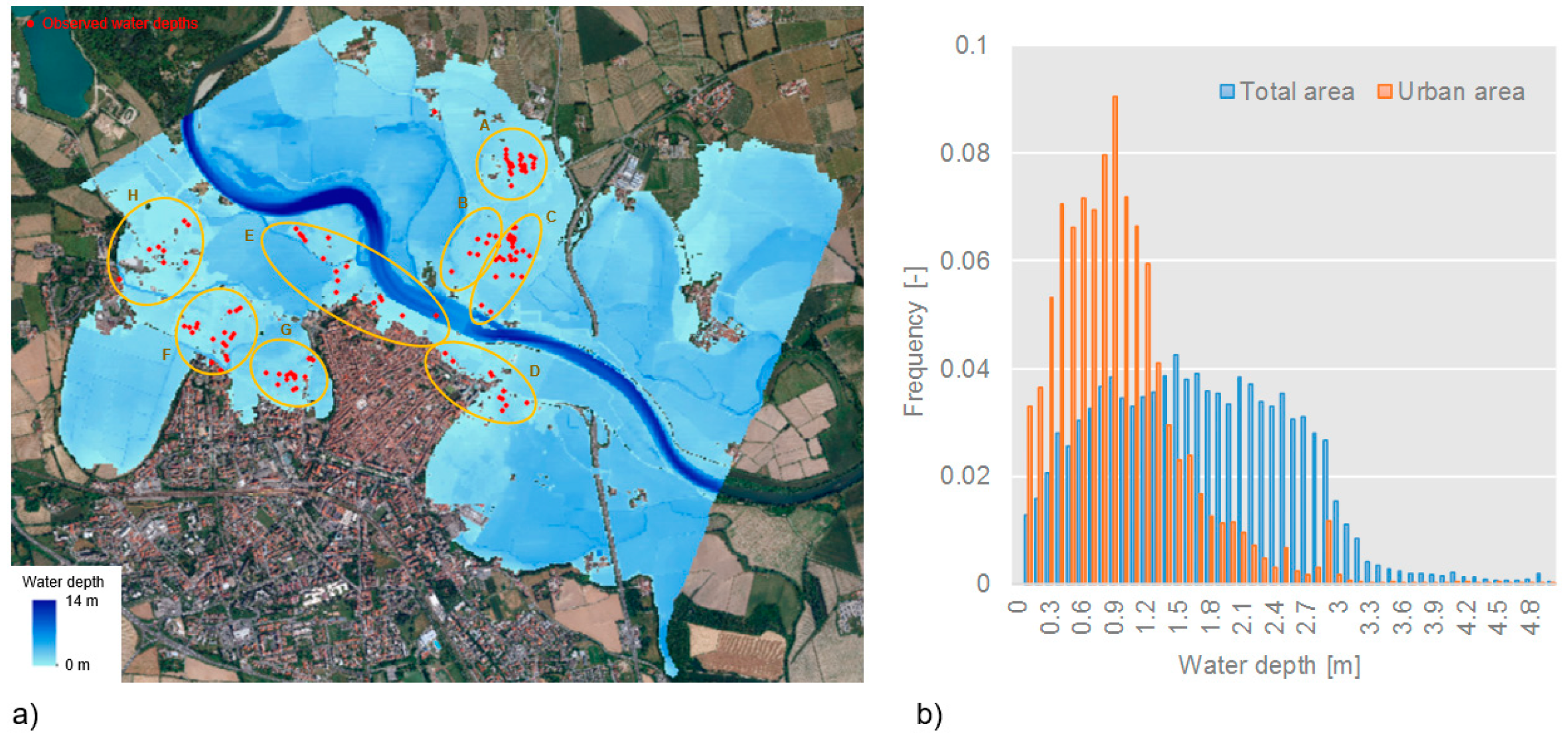
• Observed water depths in more than 260 georeferenced points within the inundated area (Figure 3a), deriving from indications provided by municipal technicians and by citizens in the damage compensation forms, as well as from interpretation of photographs taken during or immediately after the event (these water depth measurements could be affected by average errors of about 20–30 cm, given the type and quality of the observations);
• Documented oil spills in some zones of the inundated area (Figure 3d);
• Observed losses for 271 residential buildings, deriving from damage compensation forms compiled by citizens, for a total of 3.77 M€ (as of year 2002).

4. Hazard Modelling of the 2002 Adda Flood

4.1. 2D Hydraulic Model

A 2D hydraulic model was setup to reproduce the 2002 flood event and obtain a corresponding spatial distribution of water depths in the study area. The shallow-water equations were numerically integrated using the finite element method and the solver embedded in River2D [26]. The results of this model served as a benchmark for evaluating the reliability of RAPIDE.

River2D is based on the 2D, vertically averaged Saint-Venant equations expressed in conservative form, which result in a system of three equations representing the conservation of water mass and momentum in the x and y directions. The finite element method implemented in the model is based on the Streamline Upwind Petrov-Galerkin weighted residual formulation, which uses upstream biased test functions to ensure the stability of the solution under the full range of flow conditions [26].

We considered a 5.2 km long reach of the Adda River flowing by the town of Lodi. Both steady and unsteady simulations were performed, considering the peak flow of 1840 m³/s and the entire hydrograph of the event [25], respectively.

The bathymetry of the main channel was reconstructed from topographic surveys executed by the Po River Basin Authority on 14 cross-sections of the Adda River, including two bridges, while high-resolution LiDAR data from the same Authority were used for the geometry of the floodplains, extending over 13.5 km². A computational grid with a resolution of 10 m was used in the model in order to reach a satisfactory compromise between computational time, model stability and accuracy.

The model calibration was supported by the observations of water depth in the flooded area during the event, as well as by the availability of the inundation footprint (Figure 3a). The model was calibrated following a recursive procedure involving the change of the roughness coefficients attributed to channel, agricultural and urban areas (buildings were not resolved but parameterized in terms of increased roughness coefficients). The choice of the best calibration run was based on four objective functions that evaluate the effectiveness of the model in predicting water depths (the first three indicators) and the extent of the inundated area (the last one):

• the average of the differences between simulated and observed water depths (AD);
• the absolute average of the differences between simulated and observed water depths (AAD);
• the Nash-Sutcliffe Efficiency (NSE) [27], defined as:

  $$NSE=1-\frac{{\displaystyle \sum _{i=1}^n{(W{D}_{O_i}-W{D}_{S_i})}^2}}{{\displaystyle \sum _{i=1}^n{(W{D}_{O_i}-\overline{W{D}_{Oi}})}^2}}$$

  (1)

  where WD_Oi and WD_Si are, respectively, the observed and simulated water depth at location i, while $\overline{W{D}_{Oi}}$ is the mean observed water depth. The NSE may range between −∞ and 1 (goal value);
• the flood area index (FAI) [28], defined as:

  $$FAI=\frac{A^{11}}{A^{11}+A^{01}+A^{10}}$$

  (2)

  where A¹¹, A⁰¹ and A¹⁰ respectively represent the numbers of pixels for which both simulation and observation indicate “wet”, simulation indicates “wet” and observation indicates “dry”, and simulation indicates “dry” and observation indicates “wet”. The FAI may range between 0 and 1 (goal value).

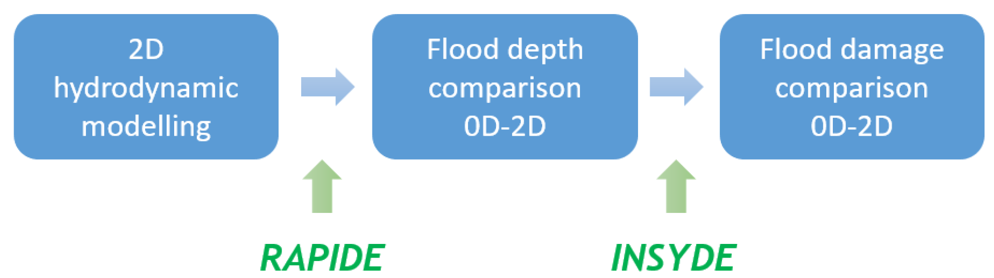
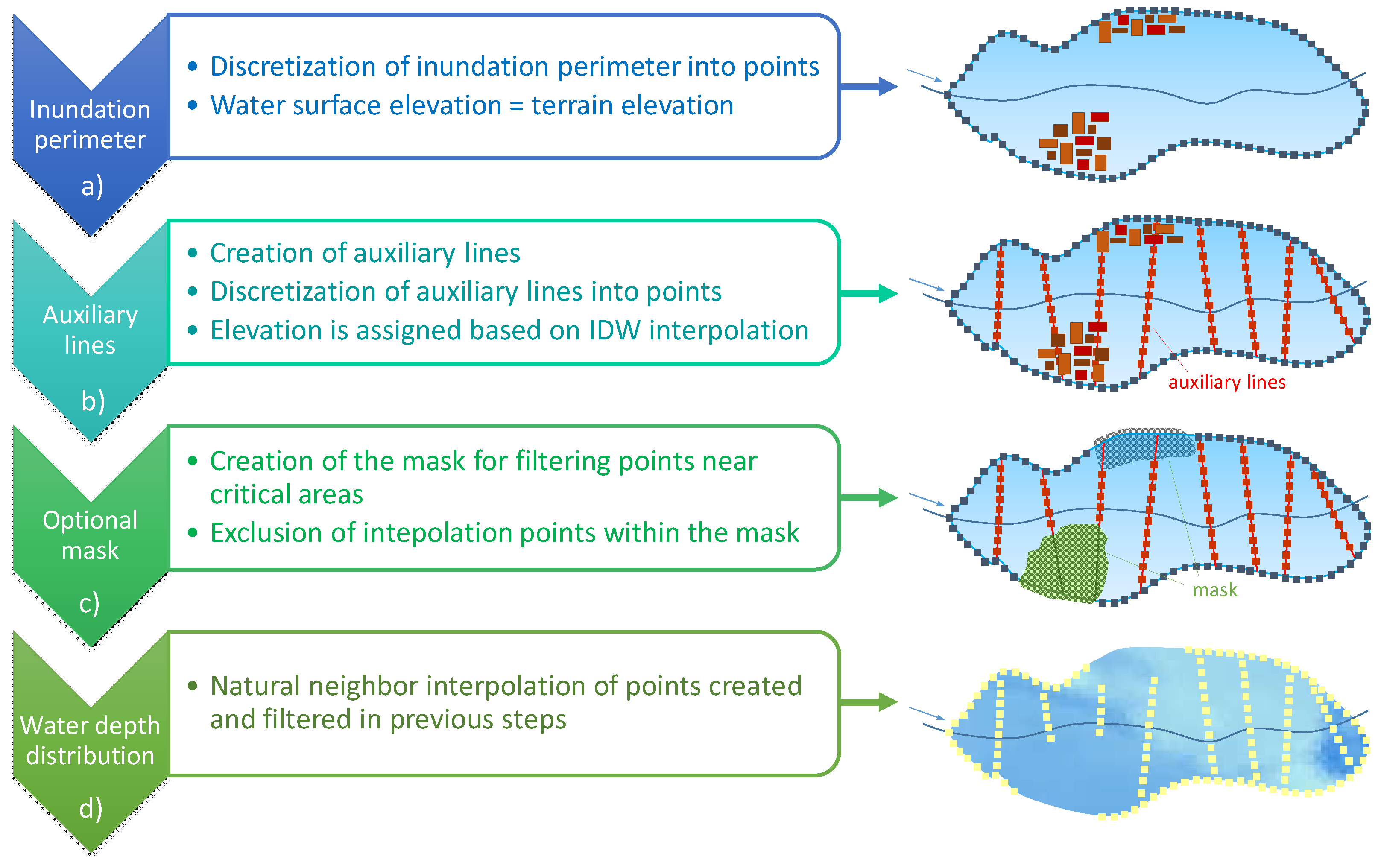
The best calibration run, optimizing a compensation of the four objective functions, was selected as the final scenario to be used as a benchmark for RAPIDE. The performance indicators for the final simulation are summarized in

Table 1. Performance indicators for the best 2D calibration run.

Indicator	Cluster
	A	B	C	D	E	F	G	H	Average
AD (m)	0.09	−0.01	0.34	0.17	−0.39	−0.18	−0.16	−0.23	−0.04
AAD (m)	0.21	0.29	0.42	0.33	0.57	0.36	0.37	0.41	0.37
NSE	0.24	0.42	−1.03	0.39	−0.04	−0.19	−0.11	−0.31	−0.18

.

The water depth-related indicators (NSE, AD, AAD) were calculated for 8 different clusters within the inundated area (as shown in Figure 4a) and then averaged; this choice was driven by the fact that registered flood depths were not evenly distributed over the flooded area, but were mainly concentrated in urban zones, as derived from observations at buildings’ locations. The clustering was performed taking into account the spatial distribution of data and the presence of discontinuities in the terrain (for example, clusters B and C are separated by a street). The AAD in the clusters ranged from 0.2 to 0.4 m, which can be considered acceptable, as observations could be affected by errors of the same magnitude. Similar considerations can be applied to the FAI (equal to 0.87), given that the inundation extent was reconstructed from interpretation of aerial photographs and descriptions of the event provided in reports. The inundation map and the histograms shown in Figure 4 denote shallow to medium water depths, with mean values of about 1.6 m, if considering the whole inundated area, and 0.9 m if selecting urban areas only. The flow velocity map (not shown) indicates a typical riverine flood, with values generally below 0.5 m/s.

4.2. RAPIDE Model

RAPIDE was applied to the 2002 Adda flood scenario and the results were compared to those provided by the 2D simulation. As shown in Section 2, the tool requires the DTM, the perimeter of the inundated area, the selection of auxiliary lines enhancing the accuracy of the spatial interpolation, and a mask for filtering points near critical urban areas or manmade structures. Therefore, in order to test the influence of the user’s choices on the results, different conditions were tested regarding:

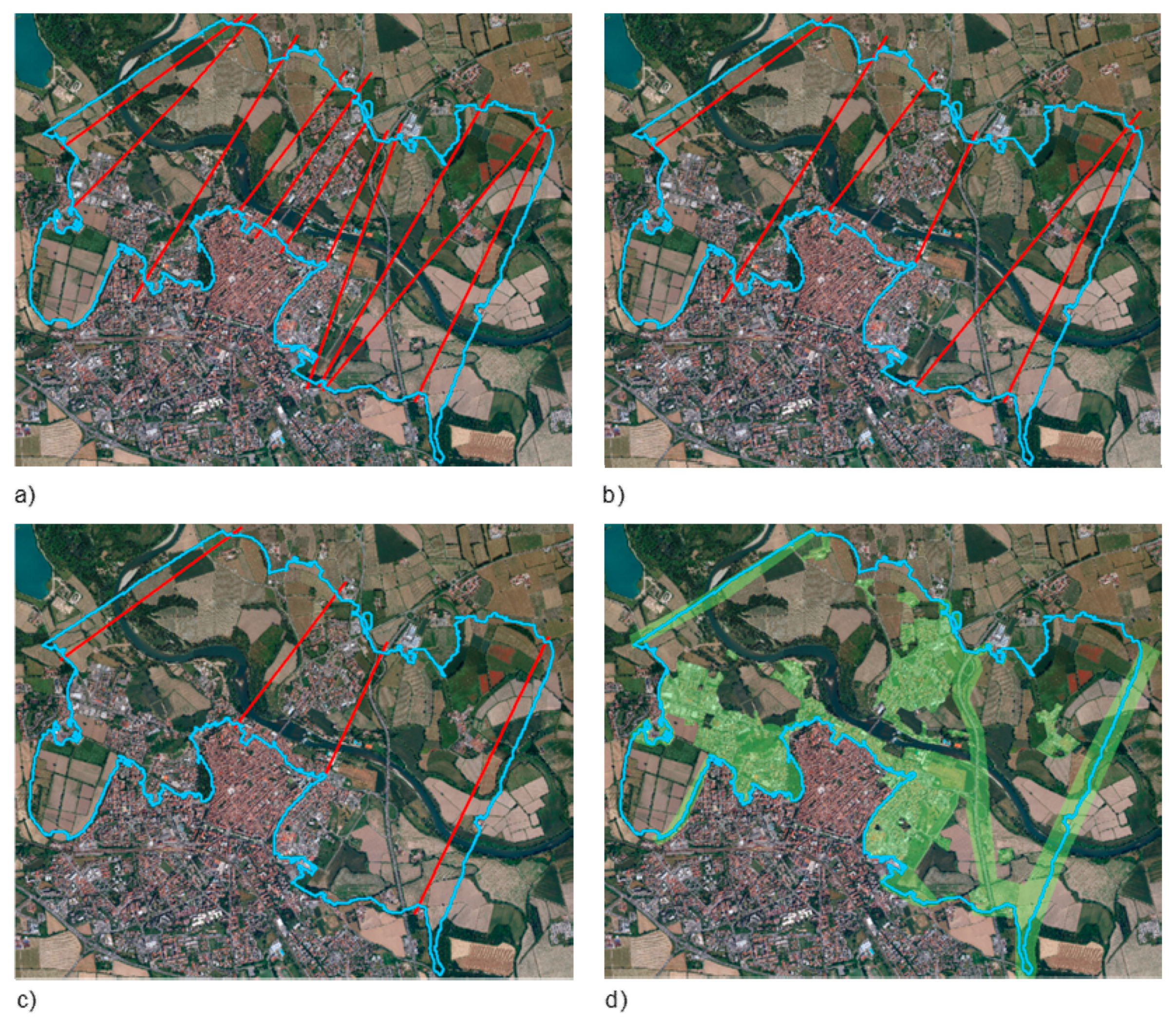
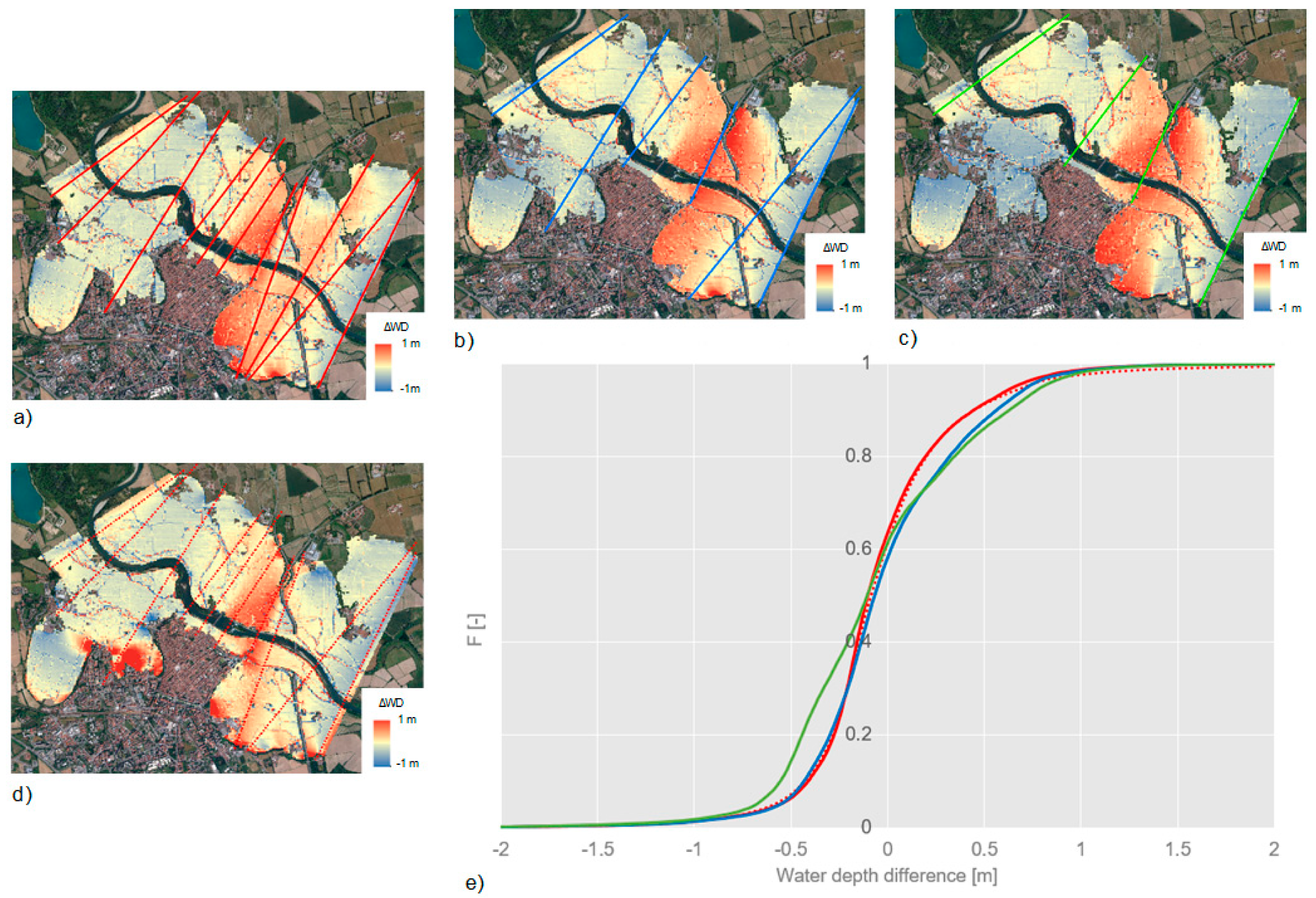
• the number of selected auxiliary lines (that is inversely proportional to the spacing between these lines): three scenarios with increasing mean spacing (from 450 m to 1.3 km, corresponding approximately to 3 and 10 times the Adda’s main channel width) were considered (i.e., ‘narrow’, ‘large’ and ‘very large spacing’ cases (Figure 5)); the last two configurations were obtained by deleting lines from the ‘narrow spacing’ case and without changing their positions;
• the use of a mask: the default condition for all the tested scenarios included the use of a polygon mask derived from the regional land-use map filtered for built-up areas (Figure 5d); the upstream and downstream boundaries of the inundated area (where it was known that water depth was not null) were masked as well; the ‘narrow spacing’ case was then tested also without the use of this mask;
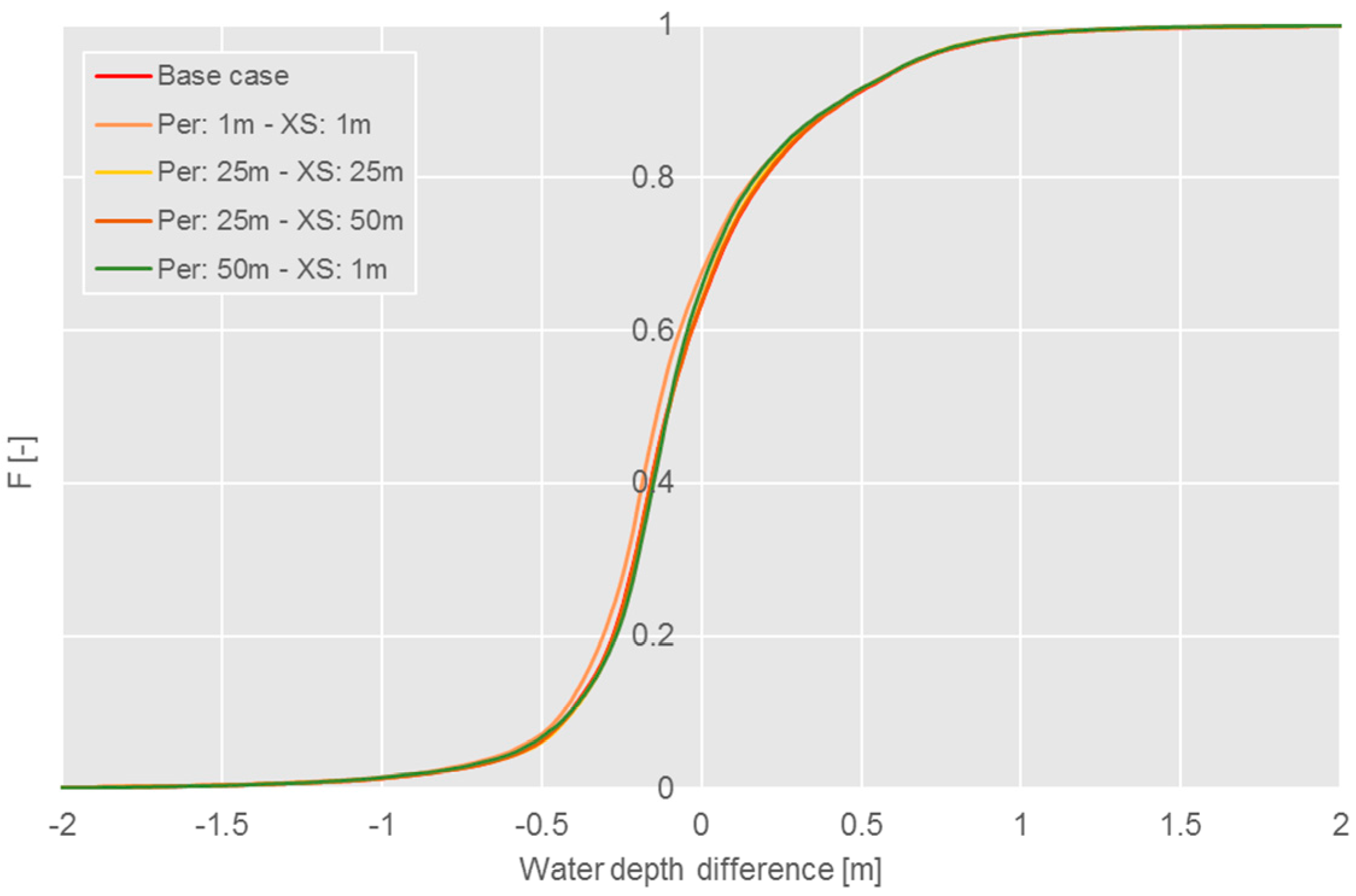
• the resolution used for the discretization of the flood perimeter and auxiliary lines: in the RAPIDE toolbox the user can change the default values for the resolution of the discretization, equal to 25 m and 1 m for flood the perimeter and auxiliary lines, respectively; based on the ‘narrow spacing’ case, different conditions were tested, varying the resolution between 1 m and 50 m for the perimeter and up to 50 m for the lines;
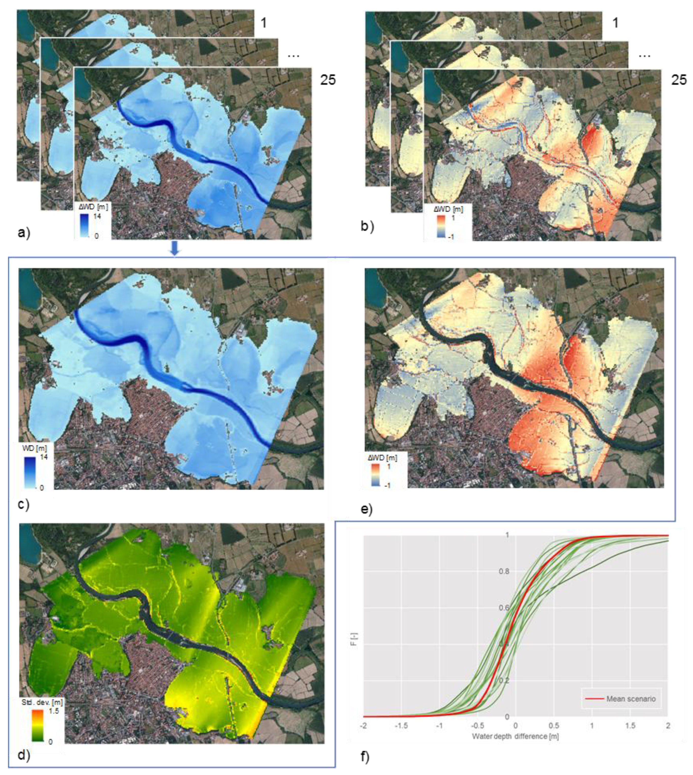
• the location of the auxiliary lines: a total of 25 configurations were generated and tested; the number of possible configurations was mainly limited by the requirements of perpendicularity to the channel axis, non-intersection with other drawn lines, intersection with the flood perimeter in two points over the external boundary and physical meaning of the lines.

The water depth maps obtained for each condition (WD_RAPIDE) were compared to the benchmark one (WD_2D) resulting from the 2D hydraulic model, by making a raster difference and then computing the cumulative density function of the differences (ΔWD = WD_RAPIDE − WD_2D). For each configuration of the sensitivity analysis, results are thus presented as maps depicting the differences between the water depths returned by RAPIDE and those simulated by the 2D model (ΔWD), and corresponding mean values and/or cumulative distribution functions of ΔWD. The mean absolute error (MAE) and the root mean squared error (RMSE) were also used as synthetic performance indicators.

Figure 6 shows the results for the base case (i.e., narrow spaced sections and mask applied) and for the other tested configurations in the sensitivity analysis related to the spacing of auxiliary lines.

Figure 6a,e reveal a median error for the base case of about −0.10 m (90th and 10th percentiles of the distribution: 0.44 m and −0.41 m, respectively), with WD_RAPIDE generally lower than WD_2D in the upstream part of the domain and opposite relationship in the second half of the reach. The results do not change drastically when using in RAPIDE less auxiliary lines for the interpolation (Figure 6b,c), even though a general worsening of the performance is observed (Figure 6e, with median ΔWD of −0.07 m and −0.10 m; 90th percentile of the distributions: 0.56 m and 0.63 m; 10th percentile of the distributions: −0.43 m and −0.55 m for the ‘large’ and ‘very large spacing’ case, respectively). Calculated MAE and RMSE values increase from 0.28 m and 0.38 m (for the base case) to 0.38 m and 0.49 m (for the ‘very large spacing’ case).

The use of the mask for filtering interpolation points does not have a substantial influence on the model’s output for the investigated case study, as highlighted by the red dotted cumulative density function almost overlapping the one obtained for the base case (MAE: 0.29 m; RMSE: 0.44 m); larger errors are identified only near a small portion of the external inundation perimeter adjacent to a built-up area, where RAPIDE produced a local water depth overestimation (Figure 6d) due to the expected problems in interpolation near urban areas when a mask is not applied.

The spatial resolution used to discretize the inundation perimeter and the auxiliary lines was also changed in the sensitivity analysis. Figure 7 demonstrates a negligible influence of this resolution, as the distributions of ΔWD for different resolutions (ranging from 1 m to 50 m for the flood perimeter and up to 50 m for the auxiliary lines) are practically identical to the one observed in the base case.

More complex results appear instead in the sensitivity analysis for the auxiliary lines’ location. As mentioned above, RAPIDE was applied to 25 configurations where the location of six lines (the line number used in the ‘large spacing’ case) was repeatedly changed. The choice of using this fixed (and relatively low) number of lines was driven by the limited sensitivity of the model to the spacing (Figure 6e). In addition, a larger spacing gives the possibility to create more test configurations while, if a higher number of lines is used, the number of possible configurations is limited by the requirements of RAPIDE (basically, the need of non-intersecting auxiliary lines). Maps of water depths (Figure 8a) and water depth differences (ΔWD) (Figure 8b) were calculated for each test case and the corresponding cumulative distribution functions were extracted as well (Figure 8f). Figure 8f clearly denotes that the lines’ location is the main influencing factor for RAPIDE’s output, with the median ΔWD values ranging from −0.20 m to 0.21 m (90th percentiles of the distributions ranging from 0.35 m to 1.40 m; 10th percentiles ranging from −0.24 m to −0.80 m). The MAE and RMSE for the configuration providing the best (worst) fit with observed water depths are equal to 0.28 m and 0.40 m (0.56 m and 0.79 m), respectively. Similarly to what is already shown in Figure 6, the analysis of the individual flood depth maps has revealed lower and more uniform ΔWD values in the upstream part of the computational domain, where maximum errors do not generally exceed ±0.5 m, as opposed to the downstream part which exhibits, for few configurations, localized overestimations (greater than 1.5 m) in the southern downstream area near a highway embankment crossing the entire domain. A final water depth map was then derived by averaging the individual rasters obtained for the different configurations (Figure 8a), thus obtaining a ‘mean scenario’ (Figure 8c). The underlying idea was that a mean scenario would compensate the possible errors introduced in the single configurations. The standard deviation map was calculated as well in order to have spatial information on the dispersion of the results (Figure 8d).

Figure 8f demonstrates that the mean scenario (red line) provides a reasonable estimate of the water elevations and depths, with tails that are wider than those for few cases but narrower than those for most cases. The 90th and 10th percentiles of the cumulative distribution of ΔWD for the ‘mean scenario’ (red line in Figure 8f) were equal to 0.54 m and −0.44 m, with MAE and RMSE values of 0.31 m and 0.41 m.

In conclusion, this sensitivity analysis demonstrates that a multiple application of RAPIDE with different locations of the auxiliary lines may lead to a reliable estimation of flood depths within an inundated area in mixed rural-urban environments, like the one investigated in this study. In addition, the use of this multirun approach can help the user in detecting possible causes of errors in the output, by comparing the water depth maps obtained from the different simulations: for instance, the reasons for possible significant differences in the results from a specific run may be attributable to an improper location of the input auxiliary lines (e.g., intersecting storage or ineffective flow areas) or local irregularities in the DTM that still need to be masked (e.g., presence in the DTM of isolated trees that may bias the interpolation).

Natural neighbor is currently the only method for spatial interpolation of flood depths implemented in the toolbox, because during the development of the method, it was observed to produce smoother surfaces that represented well the inundation features (especially if compared to spatial IDW, in line with previous literature [22,23,29]) and to lead to the smallest differences from the 2D modelled flood maps. Ordinary kriging was tested as well, and it was found to perform very similarly to natural neighbor, providing, for example, a RMSE of 0.40 m and 0.53 m in the application to the base case and the ‘very large spacing’ case of Figure 5 (0.38 m and 0.49 m obtained with natural neighbor). In general, the sensitivity analysis indicated that the location of the auxiliary lines has a much greater influence on the results than the selection of the interpolation method, although this still needs to be confirmed with additional applications to different test cases.

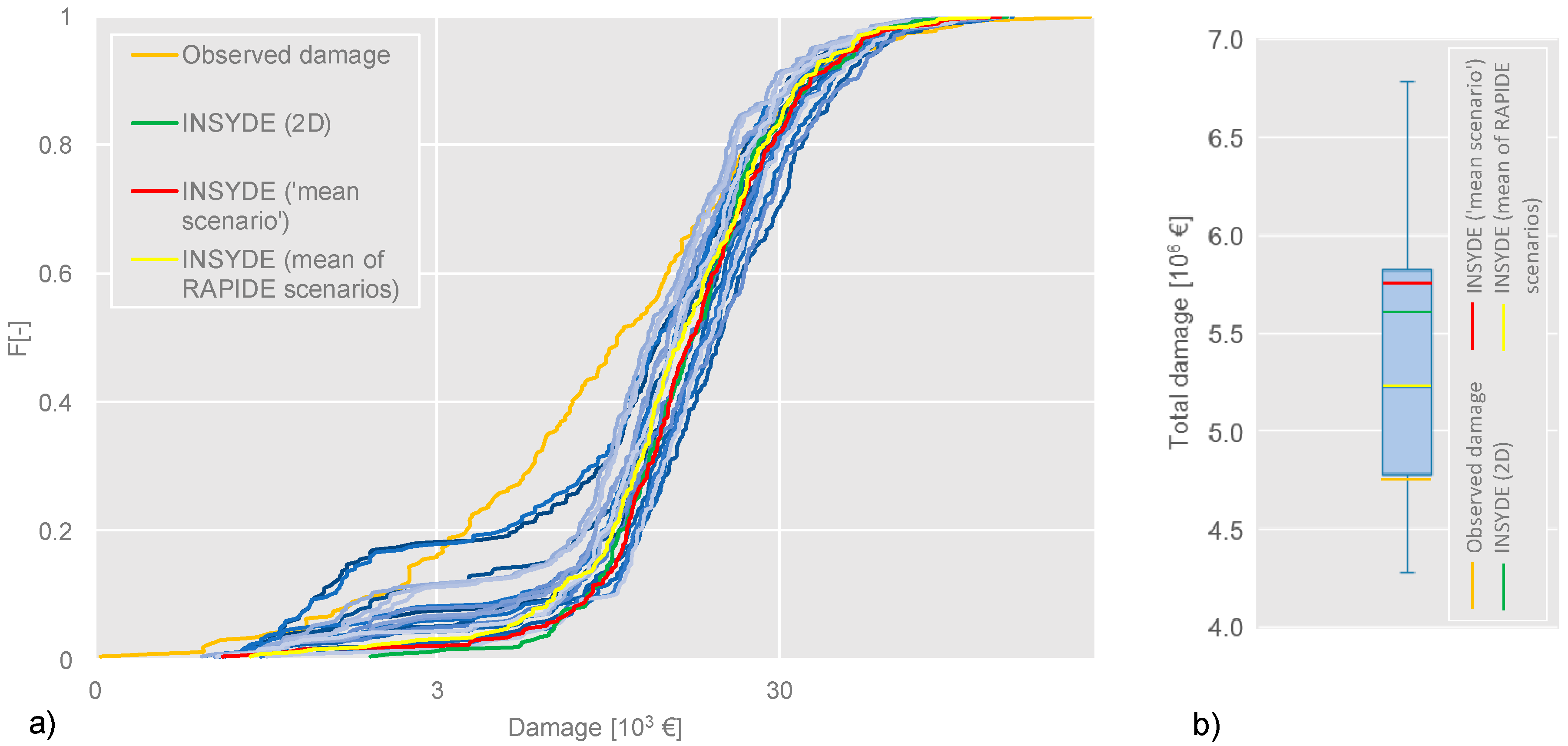
5. Damage Modelling of the 2002 Adda Flood

The inundation scenarios obtained from the application of the 2D model and RAPIDE were considered as the input hazard data for the estimation of direct damage to residential buildings consequent to the 2002 Adda flood. The main aim of the exercise was analyzing whether the variation of the hazard quantities (using a 2D hydraulic model or a 0D interpolation method) can affect damage assessment to an extent making the use of a 0D method unjustifiable.

The damage modelling was performed using INSYDE, a synthetic micro-scale multi-variable model based on an explicit component-by-component analysis of physical damage to residential buildings [24]. A previous study [30] has shown INSYDE to provide minimum errors in the calculation of expected losses for the Adda case study compared to those obtained with other existing models in the literature. In INYSDE, the flood damage is modelled by means of analytical functions that account for the damage mechanisms for each building component. The associated repair/replacement costs are also considered as a function of hazard and building characteristics. An expert-based “what-if” approach is used to develop the damage functions [24]. Despite the large number of input variables (for a total of 23 input data), the model can be also applied when the available knowledge of the flood event and building characteristics is incomplete, given the possibility of automatically considering default values for unknown parameters and of expressing some of the variables as functions of other ones, thus decreasing the number of required inputs [31].

In the present study, different data sources were used for a micro-scale characterization of residential buildings, in terms of exposure and vulnerability:

• the geometric characteristics (i.e., footprint area, external perimeter, basement area, number of floors) and finishing level of the buildings were derived from cadastral data;
• the building type (i.e., apartment, semi-detached or detached house), level of maintenance and year of construction were assigned to different buildings, based on the urban development plan of the town of Lodi;
• the building material (i.e., reinforced concrete or masonry) was assigned considering the most frequent type observed in each census zone of Lodi, based on ISTAT data, as shown in [31].

Table 2. Hazard parameters considered in INSYDE, in the case of application of the results deriving from the 2D model and RAPIDE.

Hazard Parameter	2D Model	RAPIDE
Water depth (h)	Water depth distribution as of output from 2D model	Water depth distribution as of output from RAPIDE
Flow velocity (v)	Flow velocity distribution as of output from 2D model	Default value in INSYDE (0.5 m/s)
Flood duration (d)	Default value in INSYDE (24 h)
Water quality (q)	As from documented observations during the event
Presence of sediment (s)	Default value in INSYDE (fine-grained sediment)

summarizes the hazard parameters considered as input data for INSYDE. For the characterization of water depths at building locations, we examined two different scenarios, one based on the results of the 2D hydraulic model of the flood event and one deriving from the application of RAPIDE. In the latter case, all the inundation maps resulting from the sensitivity analysis described in the previous section were tested, in order to analyze whether the user’s choices in RAPIDE implementation may significantly impact the loss prediction. As regards flow velocity, the default value implemented in INSYDE (0.5 m/s) was used in damage calculations with RAPIDE’s output since, differently from the 2D model, the tool does not provide flow velocity distribution maps; this choice is coherent with simulated flow velocities obtained by River2D, which were generally found lower than 0.5 m/s (Section 4.1). Moreover, it is worth noting that INSYDE is not significantly influenced by this parameter in case of riverine floods characterized by low velocity values [24]; this implies that all the investigated variability in the prediction of flood losses can be fully attributed to the method for the water depth estimation. Concerning the flood duration, the default value in INSYDE (24 h) was used in both scenarios because, despite the availability of the 2D unsteady run, it was not possible to simulate the full duration of the recession limb of the hydrograph, due to high computational times. The adopted value for flood duration can be regarded as representative for the event, as confirmed by testimonies given by affected citizens and considering the duration of the peak phase of the registered hydrograph (Figure 3b).

Based on INSYDE’s output (consisting of building by building loss estimates), the cumulative distribution functions of the damages as well as the total damage figures were obtained for all the hazard scenarios and compared to the observations for the 2002 Adda flood. The observed loss data were updated to year 2013 in order to make them comparable to INSYDE’s output, as the model uses 2013 price lists.

The results of the application of INSYDE to the tested hazard scenarios are presented in Figure 9a, which displays the cumulative distribution functions of observed building damages (orange line) compared to those obtained for the different simulated hazard conditions (in green for the 2D model and in shades of blue for RAPIDE). Furthermore, Figure 9b summarizes the maximum and minimum values and the interquartile range of the total damage calculated for the different configurations generated in the sensitivity analysis of RAPIDE.

The results of Figure 9 are also presented in terms of a “mean damage”, which can be obtained in two ways. In fact, since the combination of hazard and building characteristics into damage models is not linear, mean results are affected by the averaging strategy, i.e., averaging hazard or damage. The red lines in Figure 9 are obtained using the water depths extracted from the ‘mean scenario’ of RAPIDE (Figure 8c) as input data for INSYDE (thus requiring only one run of INSYDE for the mean flood scenario). The yellow lines are instead obtained by calculating damages for each single inundation scenario considered in the sensitivity analysis of RAPIDE (this approach obviously requires 25 runs of INSYDE, one for each flood scenario) and then averaging them. The corresponding total damages in Figure 9b differ by a little more than 10% (5.3 M€ and 5.7 M€), with larger total damage when INSYDE is applied to the mean scenario from RAPIDE. Expectedly, the total damage from the latter scenario is more similar than the other one to the total damage estimated using the results of the 2D model (about 5.6 M€).

Figure 9a shows that damages are generally overestimated (especially the smallest values), the same tendency being found also in the application of other damage models to the same case study [30]. The largest damage values are sometimes underestimated, even if this is partly masked in the plot by the log scale used for the horizontal axis. However, all the computed damage distribution functions fall in a quite narrow band, indicating that the loss estimates are weakly sensitive to using different hazard inputs. The variability associated to individual applications of RAPIDE (Figure 8f), depending on the choice of location and, to a lesser extent, spacing of the auxiliary lines introduced in the model, is not further enhanced by the following application of INSYDE. This means that the magnitude of the errors in flood depth prediction (<0.5 m, over mean registered water depths of about 1.5 m) produced by the application of the proposed tool does not significantly affect damage calculations.

The distributions for the two mean damages defined above are quite close to each other and similar to the one for INSYDE following the 2D hydraulic model. Furthermore, the boxplot in Figure 9b confirms that the damage estimated with the 2D hazard input falls within the resulting error range (minimum-maximum) for simulated total damage with the different runs of RAPIDE and is close to the damage estimated from the mean RAPIDE scenario. It is, therefore, argued that the water depth predictions by RAPIDE are consistent with the needs of flood damage and risk analyses.

6. Discussion and Recommendations

This paper analyzed the capabilities of a new GIS simplified model, RAPIDE, relying only on DTM and inundation perimeter, for predicting water depths over a flooded area. This rapid method (with efficient computational times, i.e., few minutes) is based on the spatial interpolation of water levels starting from the basic hypothesis that the boundary of the flooded area is characterized by null water depths. Compared to other similar 0D tools, in RAPIDE the quality of the interpolation is improved by the use of control points within the domain, which need to be located over user-determined auxiliary lines perpendicular to the river’s channel, not intersecting each other and not pertaining to ineffective or storage areas in the floodplains. Another improvement is given by the possibility of using a polygon mask for filtering interpolation points near critical zones, as built-up areas and isolated structures.

With reference to the flood event of 2002 in Lodi, that was considered as a validation case study, the availability of a detailed 2D hydraulic model and of observed loss data allowed us, on the one hand, to test the reliability of the water depth maps produced by RAPIDE and, on the other hand, to analyze whether the variability of the hazard results, due to modelling choices and simplifications in RAPIDE, may influence the assessment of direct damage to residential buildings.

The sensitivity analysis of flood depth predictions to the user’s choices has shown that the most important factor in the application of RAPIDE is the location of the auxiliary lines and, to a lesser extent, their spacing, while the resolution of the discretization of the inundated perimeter and the auxiliary lines has negligible influence on the model’s output. The method used for the spatial interpolation (natural neighbor, inverse distance weighted, or kriging) also has limited impact on the result, with the natural neighbor performing slightly better than the others. The differences between the flood depths simulated by RAPIDE and those provided by the 2D hydraulic model were generally smaller than 0.5 m, with MAE and RMSE values ranging, respectively, from 0.28 m and 0.38 m (best case) to 0.56 m and 0.79 m (worst case). These results show that RAPIDE’s performances are in line (or even better) with those demonstrated in other test cases by similar simplified tools available in the literature, as SWAM [22,23] and FwDET [21], which share the common idea of determining water levels by means of interpolation starting from the inundation perimeter and the DTM. In particular, Gatti [22] compared the results of SWAM and a 2D hydraulic model in a validation test for the 2013 flood in Olbia (Sardinia, Italy), finding a MAE ranging from 0.42 m to 0.73 m and a RMSE ranging between 0.65 m and 0.86 m (depending on modelling choices), with local large (i.e., greater than 1.5 m) overestimations in urban areas. Similarly, Cohen et al. [21], in an application of FwDET for two flood events in Texas and Colorado with average flood depths of 1.9 m and 1.3 m, reported in both cases differences of about 0.5 m between the average depths estimated by their tool and by a 2D hydraulic model, and a RMSE of 0.37–0.38 m; furthermore, they noted that even though the differences in predictions were small (<0.5 m) for a large part of the inundated area, there were some zones, especially near the boundaries of the reach, that were characterized by considerable errors (greater than 5 m). RAPIDE demonstrated comparable or better performances, limiting the observed problems of extreme overestimation in urban areas (in [22]) and underestimation near the boundaries of the flood extent (in [21]). Furthermore, the multirun application of RAPIDE with different locations of the input sections, thus defining a ‘mean scenario’, can be a feasible solution for reducing the uncertainty in flood depth estimation as well as for identifying possible causes of errors, especially in complex rural-urban environments.

The results of the application of flood inundation maps generated by RAPIDE as input data for the assessment of direct flood damage have proven that the proposed tool is appropriate for the needs of risk-based analyses for civil protection or river basin planning purposes, especially in data-scarce regions. In particular, it was found that the uncertainty due to the representation of inundation scenarios is far smaller than that related to damage modelling. Indeed, the study carried out by Galliani et al. [30] applying some damage models existing in the literature for the same case study under investigation in this work revealed that the uncertainty band inherent to the choice of the damage model is extremely large (in the order of two- to four-fold overestimation of observed building losses). Thus, damage estimation is far more sensitive to the damage model than to the model used for hazard quantification. The results of the present study and of reference [30] jointly confirm, in line with findings of previous studies [16,17,32,33], that hazard modelling is not the most important contributor to the uncertainty in the assessment of direct flood damages and risk and, therefore, that the use of rapid and simplified tools can be considered suitable in river basin and emergency planning (where, in other words, errors of the same magnitude of those registered in the use of RAPIDE are tolerable).

However, a possible limiting factor to the practical applicability of RAPIDE in the context of flood risk assessment is the need for the inundation perimeter as main input data. Indeed, as opposed to scenario reconstruction in the aftermath of an event, where information on the inundation footprint is usually available, the determination of the flood extent is one of the main outputs of flood hazard modelling towards Flood Risk Management Plans (FRMPs). In such situations, RAPIDE can be combined with the application of a 1D model, which can provide the starting interpolation points for water elevation over a series of discrete cross-sections.

In conclusion, RAPIDE is a viable tool for simplified estimates of flood hazard and risk. However, it should be remembered that RAPIDE, being a 0D model and thus not relying on the solution of physical based equations, cannot reproduce the water propagation in the floodplains (especially if characterized by a complex morphology), nor derive flow velocity or flood duration maps (which can be useful for risk assessments in the case of flash floods or for particular exposed assets, as agriculture [24,34]). In all of these cases, the classical 2D hydraulic modelling still remains the most appropriate solution.

References

1. Plate, E.J. Flood risk management for setting priorities in decision making. In Extreme Hydrological Events: New Concepts for Security; Vasiliev, O.F., van Gelder, P.H.A.J.M., Plate, E.J., Bolgov, M.V., Eds.; Springer: Dordrecht, The Netherlands, 2007; pp. 21–44. ISBN 978-1-4020-5739-7. [Google Scholar]
2. Merz, B.; Kreibich, H.; Schwarze, R.; Thieken, A. Assessment of economic flood damage. Nat. Hazards Earth Syst. Sci. 2010, 10, 1697–1724. [Google Scholar] [CrossRef]
3. Armenakis, C.; Du, E.X.; Natesan, S.; Persad, R.A.; Zhang, Y. Flood risk assessment in urban areas based on spatial analytics and social factors. Geosciences 2017, 7, 123. [Google Scholar] [CrossRef]
4. Lugeri, N.; Kundezewicz, Z.W.; Genovese, E.; Hochrainer, S.; Radziejewski, M. River flood risk and adaption in Europe—Assessment of the present status. Mitig. Adapt. Strateg. Glob. Chang. 2010, 15, 621–639. [Google Scholar] [CrossRef]
5. Horrit, M.S.; Bates, P.D. Predicting floodplain inundation: Raster-based modelling versus the finite-element approach. Hydrol. Process. 2001, 15, 825–842. [Google Scholar] [CrossRef]
6. Horrit, M.S.; Bates, P.D. Evaluation of 1D and 2D numerical models for predicting river flood inundation. J. Hydrol. 2002, 268, 87–99. [Google Scholar] [CrossRef]
7. Büchele, B.; Kreibich, H.; Kron, A.; Thieken, A.; Ihringer, J.; Oberle, P.; Merz, B.; Nestmann, F. Flood-risk mapping: Contribution towards an enhanced assessment of extreme events and associated risks. Nat. Hazards Earth Syst. Sci. 2006, 6, 485–503. [Google Scholar] [CrossRef]
8. Pender, G. Briefing: Introducing the flood risk management research consortium. In Proceedings of the Institution of Civil Engineers—Water Management; Thomas Telford Ltd.: London, UK, 2006; Volume 159, pp. 3–8. [Google Scholar]
9. Woodhead, S.; Asselman, N.; Zech, Y.; Soares-Frazão, S.; Bates, P.; Kortenhaus, A. Evaluation of Inundation Models-Limits and Capabilities of Models. FLOODSite Report T08-07-01. 2007. Available online: http://www.floodsite.net/html/partner_area/project_docs/T08_07_01_Inundation_Model_Evaluation_M8_1_V1_7_P15.pdf (accessed on 7 December 2018).
10. Teng, J.; Jakeman, A.J.; Vaze, J.; Croke, B.F.; Dutta, D.; Kim, S. Flood inundation modelling: A review of methods, recent advances and uncertainty analysis. Environ. Modell. Softw. 2017, 90, 201–216. [Google Scholar] [CrossRef]
11. Vojinovic, Z.; Tutulic, D. On the use of 1D and coupled 1D-2D modelling approaches for assessment of flood damage in urban areas. Urban Water J. 2009, 6, 183–199. [Google Scholar] [CrossRef]
12. de Moel, H.; van Alphen, J.; Aerts, J.C.J.H. Flood maps in Europe—Methods, availability and use. Nat. Hazards Earth Syst. Sci. 2009, 9, 289–301. [Google Scholar] [CrossRef]
13. Ward, P.J.; Jongman, B.; Weiland, F.S.; Bouwman, A.; van Beek, R.; Bierkens, M.F.; Ligtvoet, W.; Winsemius, H.C. Assessing flood risk at the global scale: Model setup, results, and sensitivity. Environ. Res. Lett. 2013, 8, 044019. [Google Scholar] [CrossRef]
14. McGrath, H.; Bourgon, J.F.; Proulx-Bourque, J.S.; Nastev, M.; El Ezz, A.A. A comparison of simplified conceptual models for rapid web-based flood inundation mapping. Nat. Hazards 2018, 93, 905–920. [Google Scholar] [CrossRef]
15. Autoritàdi Bacino del Fiume, P. Piano per la Valutazione e la Gestione del Rischio di Alluvioni. Mappatura della Pericolosità e Valutazione del Rischio; Report II.A; Autorità di Bacino del Fiume Po: Parma, Italy, 2016; 29p. [Google Scholar]
16. Scorzini, A.R.; Leopardi, M. River basin planning: From qualitative to quantitative flood risk assessment: The case of Abruzzo Region (central Italy). Nat. Hazards 2017, 88, 71–93. [Google Scholar] [CrossRef]
17. Teng, J.; Vaze, J.; Dutta, D.; Marvanek, S. Rapid inundation modelling in large floodplains using LiDAR DEM. Water Resour. Manag. 2015, 29, 2619–2636. [Google Scholar] [CrossRef]
18. Lhomme, J.; Sayers, P.; Gouldby, B.; Samuels, P.; Wills, M.; Mulet-Marti, J. Recent development and application of a rapid flood spreading method. In Flood Risk Management: Research and Practice; Samuels, P., Huntington, S., Allsop, W., Harrop, J., Eds.; Taylor & Francis Group: London, UK, 2008. [Google Scholar]
19. Nobre, A.D.; Cuartas, L.A.; Hodnett, M.; Rennó, C.D.; Rodrigues, G.; Silveira, A.; Waterloo, M.; Saleska, S. Height Above the Nearest Drainage—A hydrologically relevant new terrain model. J. Hydrol. 2011, 404, 13–29. [Google Scholar] [CrossRef]
20. Zhang, J.; Huang, Y.F.; Munasinghe, D.; Fang, Z.; Tsang, Y.P.; Cohen, S. Comparative analysis of inundation mapping approaches for the 2016 flood in the Brazos River, Texas. J. Am. Water Resour. Assoc. 2018, 54, 820–833. [Google Scholar] [CrossRef]
21. Cohen, S.; Brakenridge, G.R.; Kettner, A.; Bates, B.; Nelson, J.; McDonald, R.; Huang, Y.F.; Munasinghe, D.; Zhang, J. Estimating floodwater depths from flood inundation maps and topography. J. Am. Water Resour. Assoc. 2017, 54, 847–858. [Google Scholar] [CrossRef]
22. Gatti, F. Stima del Rischio Alluvionale per le Attività Economiche: Il Caso Studio di Olbia (OT). Master’s Thesis, Università degli Studi di Milano, Milan, Italy, 2016; p. 91. [Google Scholar]
23. Pastormerlo, M. SWAM (Surface Water Analysis Method): Un Metodo Speditivo per la Modellazione di un Evento Alluvionale. Master’s Thesis, Università degli Studi di Milano, Milan, Italy, 2016; p. 112. [Google Scholar]
24. Dottori, F.; Figueiredo, R.; Martina, M.L.V.; Molinari, D.; Scorzini, A.R. INSYDE: A synthetic, probabilistic flood damage model based on explicit cost analysis. Nat. Hazards Earth Syst. Sci. 2016, 16, 2577–2591. [Google Scholar] [CrossRef]
25. Rossetti, S.; Cella, O.W.; Lodigiani, V. Studio idrologico-idraulico del tratto del f. adda inserito nel territorio comunale. In Relazione Idrologico-Idraulica; Atti del P.G.T. del comune di Lodi: Lodi, Italy, 2010; p. 101. [Google Scholar]
26. Steffler, P.M.; Blackburn, J. River2D—Two-Dimensional Depth Averaged Model of River Hydrodynamics and Fish Habitat; University of Alberta: Edmonton, AB, Canada, 2002. [Google Scholar]
27. Nash, J.E.; Sutcliffe, J.V. River flow forecasting through conceptual models part I—A discussion of principles. J. Hydrol. 1970, 10, 282–290. [Google Scholar] [CrossRef]
28. Dung, N.V.; Merz, B.; Bárdossy, A.; Thang, T.D.; Apel, H. Multi-objective automatic calibration of hydrodynamic models utilizing inundation maps and gauge data. Hydrol. Earth Syst. Sci. 2011, 15, 1339–1354. [Google Scholar] [CrossRef] [Green Version]
29. Dressler, M. Art of Surface Interpolation; Technical University of Liberec Faculty of Mechatronics and Interdisciplinary Engineering Studies: Liberec, Czech Republic, 2009. [Google Scholar]
30. Galliani, M.; Scorzini, A.R.; Molinari, D.; Minucci, G. Flood damage model validation and the level of detail of input data quality: The case of the 2002 flood in Lodi (northern Italy). In Proceedings of the 5th IAHR Europe Congress, Trento, Italy, 12–14 June 2018. [Google Scholar]
31. Molinari, D.; Scorzini, A.R. On the influence of input data quality to flood damage estimation: The performance of the INSYDE model. Water 2017, 9, 688. [Google Scholar] [CrossRef]
32. Freni, G.; La Loggia, G.; Notaro, V. Uncertainty in urban flood damage assessment due to urban drainage modelling and depth–damage curve estimation. Water Sci. Technol. 2010, 61, 2979–2993. [Google Scholar] [CrossRef]
33. de Moel, H.; Aerts, J.C.J.H. Effect of uncertainty in land use, damage models and inundation depth on flood damage estimates. Nat. Hazards 2011, 58, 407–425. [Google Scholar] [CrossRef]
34. Brémond, P.; Grelot, F.; Agenais, A.L. Review Article: Economic evaluation of flood damage to agriculture—Review and analysis of existing methods. Nat. Hazards Earth Syst. Sci. 2013, 13, 2493–2512. [Google Scholar] [CrossRef]
Figure 1. Workflow scheme of the paper.
Water 10 01805 g001
Figure 2. Schematization of the GIS processes in RAPIDE.
Water 10 01805 g002
Figure 3. 2002 Adda river flood in the town of Lodi: (a) Observed flood footprint and location of observed water depths; (b) Observed flood hydrograph at the ancient bridge (the hydrometer is depicted by the green point in panel a); (c) Example of available aerial photographs taken during the event; (d) Observed oil spill in a part of the inundated area.
Water 10 01805 g003
Figure 4. Results of the 2D model for the 2002 Adda flood: (a) Flood depth map, with indication of clusters considered in the calibration of the model; (b) Distributions of water depths in the total inundated area and urban areas only.
Water 10 01805 g004
Figure 5. Cases considered in a sensitivity analysis of RAPIDE results to the spacing between auxiliary lines and the use of a mask: (a) ‘Narrow spacing’ case; (b) ‘Large spacing’ case; (c) ‘Very large spacing’ case; (d) Mask for filtering interpolation points in urban areas.
Water 10 01805 g005
Figure 6. Results for the sensitivity of RAPIDE results to line spacing and use of the mask. Maps of ΔWD for: (a) ‘Narrow spacing’ (red); (b) ‘Large spacing’ (blue); (c) ‘Very large spacing’ (green); (d) ‘Narrow spacing’ without a mask (red dotted); (e) Cumulative density functions of ΔWD for the four cases.
Water 10 01805 g006
Figure 7. Sensitivity of RAPIDE results to the discretization resolution of the flood perimeter and the auxiliary lines (‘Per’ and ‘XS’ in the legend, respectively). Cumulative density functions of ΔWD for the different resolutions considered.
Water 10 01805 g007
Figure 8. Sensitivity analysis of RAPIDE results to the location of auxiliary lines: (a) Water depth maps for the 25 tested configurations; (b) ΔWD maps for 25 tested configurations; (c) Water depth map for the ‘mean scenario’; (d) Map of standard deviations of water depth for the ‘mean scenario’; (e) ΔWD maps for the ‘mean scenario’; (f) Cumulative density functions of ΔWD for the 25 considered configurations (green lines) and the ‘mean scenario’ (red line).
Water 10 01805 g008
Figure 9. Results of damage modelling (loss data updated to year 2013). (a) Cumulative density functions of simulated (green: 2D model; shades of blue: RAPIDE; red: ‘mean scenario’ of RAPIDE; yellow: mean damage calculated from RAPIDE scenarios) versus observed losses for the different tested hazard configurations. (b) Boxplot of total damage calculated for the different configurations generated in the sensitivity analysis of RAPIDE (blue with yellow mean), together with the total damages for the other estimates.
Water 10 01805 g009