Effect of Density and Total Weight on Flow Depth, Velocity, and Stresses in Loess Debris Flows
by
 ,
,
Heping Shu
1,2, 
Jinzhu Ma
1,*,
Haichao Yu
1,
Marcel Hürlimann
2,
Peng Zhang
3,
Fei Liu
1 and
Shi Qi
1 1
Key Laboratory of Western China’s Environmental Systems (Ministry of Education), College of Earth and Environmental Sciences, Lanzhou University, 222 South Tianshui Road, Lanzhou 730000, China
2
Division of Geotechnical Engineering and Geosciences, Department of Civil and Environmental Engineering, UPC BarcelonaTECH, 08034 Barcelona, Spain
3
Hubei Key Laboratory of Disaster Prevention and Mitigation, China Three Gorges University, Yichang 443002, China
*
Author to whom correspondence should be addressed.
Water 2018, 10(12), 1784; https://doi.org/10.3390/w10121784
Submission received: 5 November 2018
/
Revised: 18 November 2018
/
Accepted: 3 December 2018
/
Published: 5 December 2018
(This article belongs to the Special Issue Flood Risk Analysis and Management from a System's Approach)
Abstract
:Debris flows that involve loess material produce important damage around the world. However, the kinematics of such processes are poorly understood. To better understand these kinematics, we used a flume to measure the kinematics of debris flows with different mixture densities and weights. We used sensors to measure pore fluid pressure and total normal stress. We measured flow patterns, velocities, and depths using a high-speed camera and laser range finder to identify the temporal evolution of the flow behavior and the corresponding peaks. We constructed fitting functions for the relationships between the maximum values of the experimental parameters. The hydrographs of the debris flows could be divided into four phases: increase to a first minor peak, a subsequent smooth increase to a second peak, fluctuation until a third major peak, and a final continuous decrease. The flow depth, velocity, total normal stress, and pore fluid pressure were strongly related to the mixture density and total mixture weight. We defined the corresponding relationships between the flow parameters and mixture kinematics. Linear and exponential relationships described the maximum flow depth and the mixture weight and density, respectively. The flow velocity was linearly related to the weight and density. The pore fluid pressure and total normal stress were linearly related to the weight, but logarithmically related to the density. The regression goodness of fit for all functions was >0.93. Therefore, these functions are accurate and could be used to predict the consequences of loess debris flows. Our results provide an improved understanding of the effects of mixture density and weight on the kinematics of debris flows in loess areas, and can help landscape managers prevent and design improved engineering solutions.
1. Introduction
Debris flows are common in mountainous areas [1,2,3,4,5]. They occur when masses of sediment on a slope become saturated with water and are then agitated (e.g., by heavy runoff or an earthquake), causing them to rush down the slope under the influence of gravity [6,7,8]. Debris flows can denude soil and rock, and are deposited in floodplains and alluvial fans at the base of the slope, where people and infrastructure are often concentrated [9,10,11,12]. Recently, with the ongoing increase in land exploitation required to support growing populations and an increasing frequency of extreme precipitation events due to global warming, debris flow disasters have become increasingly frequent in many regions of the world [13,14,15,16]. These events threaten residents and their societal infrastructures [17,18,19,20]. This is especially true for residents of China’s northwestern loess region [21,22], an area with widely distributed steep slopes where surface runoff occurs very rapidly. These slopes have become a serious problem for managers of soil erosion [23], and debris flow hazards have proliferated in recent decades throughout China’s loess areas [16,24]. Therefore, as the risks posed by debris flows have increased, it has become increasingly urgent to understand the kinematics of these debris flows to guide the design of preventative engineering measures [5,25].
Mitigating or preventing losses of life and disruption of societal development are critical [26]. To prevent the dam age associated with debris flows, numerous types of preventative approaches have been developed [5,27]. These can be divided into two main categories: structural and non-structural measures. The former category includes check dams [28,29,30], drainage channels [31,32], flexible net dams [33,34], and debris-flow basins [35]; the latter include warning and evacuation systems and safer land use policies, as well as retrofitting buildings to improve their resistance to flows [36,37]. However, to enhance the effectiveness of preventative structural measures, it’s important to understand the kinematics of debris flows [38,39].
To understand these kinematics, a variety of field observations have been carried out. Suwa et al. built an observation system to detect the dynamic pressure created by debris flows in Japan [40]. Hu et al. studied the peak impact of debris flows from 1973 to 2004 in the Jiangjia Ravine of China [41]. Wendeler et al. studied debris flow events in 2006 that acted on the barrier system at the Illgraben torrent observation station in Switzerland using different measurement facilities [42]. Hürlimann et al. detected six debris flows and 11 floods between 2009 and 2012 at a field station in the Pyrenees (Spain) [43]. In recent years, multi-temporal LiDAR datasets have been used to monitor debris flows [44,45,46]. However, although field monitoring is an efficient method for studying the kinematics of debris flows, there are limits to its ability to monitor and model flow behaviors [25,47,48]; debris flows are characterized by a rapid onset, a short duration, an infrequent and unpredictable occurrence, and high destructive potential [49]. Moreover, natural debris flows have been monitored only in a few high-frequency debris flows [50,51,52,53]. In contrast, controlled experiments using devices such as flumes can be repeated many times, using easily controlled variables such as the flow velocity, flow depth, and pore pressure. This makes it easy to replicate the experimental results [54,55].
For these reasons, flume experiments have become a popular tool for studying the kinematics of debris flows and their underlying mechanisms [56,57,58]. Egashira et al. studied the relationship between the particle size distribution of bed sediments and the erosion rate caused by debris flows by using flume tests [59]. Haas et al. used flume tests to investigate the effects of clay content on runout of the debris flow, and found a positive relationship between the clay content and runout, but also found that too much clay produced a viscous flow that reduced the runout [49]. Wang et al. studied the characteristics of viscous debris flows in drainage channels in a flume experiment, and found that the velocity of the viscous debris flow increased with increasing slope of the channel [5]. In addition, some tests have been conducted to study debris flow processes in loess areas, where the strongly sorted, fine-grained sediments are highly vulnerable to erosion and the creation of debris flows. Acharya et al. analyzed post-failure sediment yields during laboratory-scale soil erosion and shallow landslide experiments with a silty loess in New Zealand and found that the peak sediment yields were related to landslide occurrence [60]. Yuan et al. studied the motion characteristics (velocity and intermittent debris flows) and deposition parameters (length, width, and area) of mud flows using a flume model in the loess area of China [23]. Peng et al. simulated submersion in a typical debris flow in the Loess Plateau based on the Hydrologic Engineering Center’s River Analysis System (HEC-RAS), Geospatial Extension on Hydrologic Engineering Center’s River Analysis System (HEC-GeoRAS), and Soil and Water Assessment Tool (SWAT) results, and used a hydrological model to determine the critical rainfall threshold for initiation of a debris flow [61]. These achievements focused on deposition and entrainment, and did not comprehensively study the kinematics of the debris flows, especially in the flow zone. China’s Loess Plateau is the country’s most typical loess region [24], but despite the unique characteristics of this loess, few studies have been performed to describe the kinematics of the debris flows that occur in this region [62]. Thus, research on debris flows in the Loess Plateau is still in an elementary stage [62,63,64].
The main goal of this study was to improve our understanding of the kinematics of debris flows by analyzing data from flume experiments performed with Chinese loess material. We hypothesized that the key parameters that describe loess debris flows (flow depth, flow velocity, total normal pressure, and pore fluid pressure) would show strong and statistically significant relationships to the weight and density of each debris flow mixture. First, we describe the experimental flume, sample preparation, and the measurement techniques. Next, we used the abovementioned experimental parameters to evaluate the flow kinematics of the experimental debris flows. Finally, we discuss the relationships between the experimental results and experimental factors and develop equations to simulate the results of our flume studies so that the equations can be applied to natural debris flows. The results of our research improve understanding of the effects of sediment density and weight on the movement and deposition of debris flows in China’s loess area, and provide parameter values that can improve engineering design to prevent or mitigate debris flows.
2. Experimental Materials and Sample Preparation
To understand the kinematics of debris flows, the dynamic conditions used in data collection should be carefully controlled during the experiment. In this section, we describe our use of the similarity principle (i.e., ensuring that our laboratory-scale system behaves similarly to the real-world system being modeled) to ensure that the parameter values are realistic. We then describe the experimental apparatus and sample preparation used to control the experimental conditions.
2.1. Similarity Principle
Dimensional analysis is an important way to understand the physical links and relationships among the factors involved in a natural phenomenon or an engineering problem [58,65]. Dimensional analysis can clearly reveal the relationships between experimental results and experimental factors [7,58,66]. In the flume tests that we used in the present study, we accounted for the following experimental factors that describe the distribution of the flow density: the spatial coordinates (x, y), where x and y represent the distances parallel to the flume and perpendicular to the flow direction, respectively; volume of the debris flow (V0); characteristic depth of the fluid (h); characteristic diameter of the particles (d); channel length (L); channel width (W); slope angle (α); fluid density (ρf); density of solid material (ρs); dynamic viscosity coefficient (μ); gravitational acceleration (g); elastic modulus of grain (Es); coefficient of friction (c); initial flow velocity (v0). The distribution of the flow velocity can be expressed as follows:
We selected ρf, v0, and L as a unit system:
It is necessary to define some additional functions that describe the flow kinematics [58,67]:
where Re is the Reynolds number, which represents the ratio of inertial forces to viscosity; Fr is the Froude number, which represents the ratio of inertial forces to gravitational forces; and ε represents the ratio of the fluid depth to channel length. The dimensionless function format of flow velocity can then be obtained by using similarity theory:
These two equations represent the similarity equations for the flow field for a two-phase debris flow (here, sediment and water) that is driven by gravity. In the model and in practice, it is necessary to satisfy the dimensionless is equal.
In addition, Re and Fr appear in the distribution function for the dynamic characteristics, and must be equal in the model being developed and the actual process it represents. To achieve this goal, it’s necessary to build a model of the study system that has the same scale as the system, and this is unrealistic in practice [58]. To achieve accurate experimental results, similarity methods are used [58]. To meet this goal for the geometric similarity and kinematic similarity, Re and Fr are often used [25,58]. Because the gravitational force is one of the most important driving forces in flume experiments [58], we adopted Fr as the research object.
2.1.1. Geometric Similarity
We used the following equation to achieve geometric similarity:
where γl is the length ratio, la is the length of the actual, and lf is the length of the flume.
2.1.2. Material Similarity
We used the following equation to achieve material similarity:
where is the ratio of the density of the solid material to the fluid density for the model, is the ratio of the density of the solid material to the fluid density for the actual. We changed the fluid density during the flume experiment to measure the consequences.
2.1.3. Velocity Similarity
We used the following equation to achieve similarity for the flow velocity:
Therefore, we can achieve velocity similarity:
In addition,
Hence, we can also obtain the V0 similarity ratio.
2.2. Experimental Apparatus
The experimental flume apparatus consists of three components (Figure 1). The first is a hopper that was 1.2 m wide at the top with a side length of 0.2 m. The bottom of the hopper is a square hole equipped with a gate composed of a steel plate, which was installed so that it could be pulled away rapidly to ensure that all of the material rushed downward simultaneously. The second component is a rectangular flume with an inclination of 15° from the horizontal that is 0.4 m wide, 0.5 m deep, and 5 m long. The sides of the flume are made of smooth 10-mm-thick glass, and the bottom is a steel plate, while relatively coarse red bricks were placed along the flume bottom to resemble a natural channel. This section of the apparatus is monitored by three total normal stress sensors (FBG Load Cell, Surrey, UK) installed in the flume at upstream (S1), midstream (S2), and downstream (S3) positions to monitor the total normal stress during the debris flow. Three pore fluid-pressure sensors (FBG Load Cell, Surrey, UK) are installed at the same positions, and were labeled P1, P2, and P3, respectively. In addition, a laser range finder (LDM 41A, Rostock, Germany) was used to record the debris flow depths in the middle part of the channel at 30 cm downstream from monitoring point S2. All these sensors were connected to a datalogger, and their outputs were recorded at a frequency of 5 Hz. The third component of the apparatus is the accumulation section, which was a horizontal plate 3 m long and 2 m wide. A 20 cm × 20 cm square grid was drawn on the plate, and two digital cameras (one positioned to record motion in the flume and the other positioned to record motion on the accumulation section) were used to record videos of the experiments. These videos were used to determine the mean debris flow frontal velocity, which was calculated as follows:
where V (m/s) is the debris flow velocity, Δl (m) is the length of the flume, and Δt is the elapsed time (s).
2.3. Sample Preparation
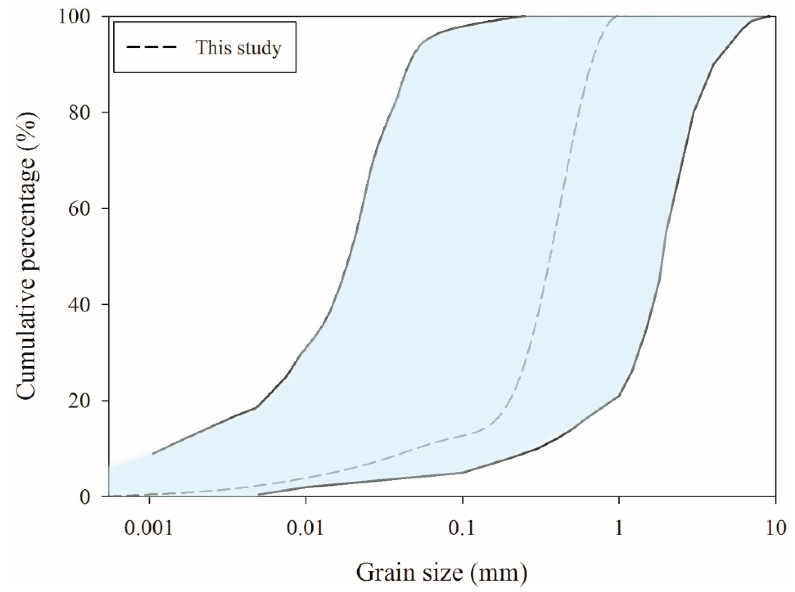
The soil materials were obtained from the Dasha Gully, Lanzhou City (103°49′ E, 36°03′ N), Gansu Province, China. To ensure that all particles could flow smoothly out of the hopper and through the flume, where the sensors were installed, we passed the samples through a 20 mm × 20 mm steel mesh to exclude particles with diameters exceeding 20 mm. The grain size distribution of the experimental sample was measured at the Key Laboratory of Western China’s Environmental Systems at Lanzhou University, using a Mastersizer 2000 (Malvern Instruments, Malvern, UK) laser diffractometer (Figure 2). The clay, silt, fine sand, medium sand, and coarse sand [68] contents were 1.0%, 9.1%, 22.2%, 47.1%, and 20.6%, respectively. The median diameter (d5) was 0.36 mm. Prior to conducting the experiment, the mixtures were prepared according to the required densities (including 1500 kg/m3, 1650 kg/m3, 1800 kg/m3, 1900 kg/m3, 2050 kg/m3, 2100 kg/m3, and 2300 kg/m3) and total weights (including 200 kg, 300 kg, 400 kg, and 500 kg).
We performed 28 experiments with different combinations of density and weight. To confirm that the equipment worked well and to improve the accuracy of the acquired data, we rinsed the apparatus with clean water to remove any remaining sediments before the start of each experiment. We then prepared the mixture and placed it in the hopper. Next, we checked the monitoring equipment to ensure that it was operating properly, and then began the experiment. After each test, we cleaned the experimental area again and analyzed the experimental data to confirm that there were no problems.
3. Results and Discussion
3.1. General Flow Patterns
Figure 3 shows the typical flow patterns in two representative experiments. Once the gate of the hopper was opened, the surface of the debris flow fluctuated considerably at the inlet section of the channel, but remained relatively stable throughout the flume. At the outlet, the cross-sectional area of the debris flow fluctuated, because the flow moved quickly into the accumulation plate. The samples with a lower density flowed faster than the samples with higher densities (Figure 3).
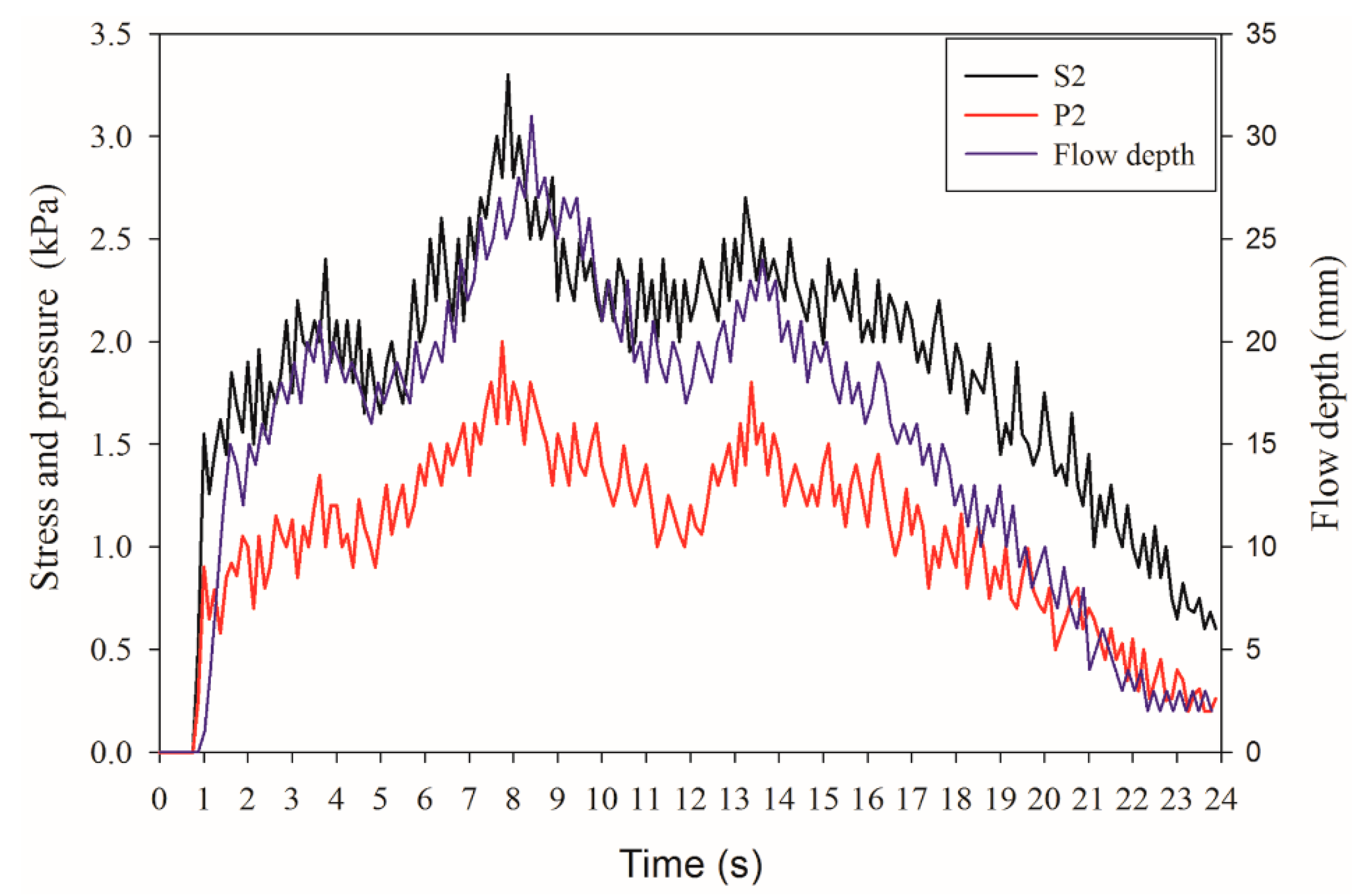
The flow depth, total normal stress, and pore fluid pressure were measured during each test, and showed that the hydrograph could be divided into four phases (Figure 4). These resemble the phases described in previous papers [6,68,72], and agree with the results of field observations [50,73,74]. The first phase represented increasing flow that rapidly reached a first peak as the mixture rushed into the flume, and the discharge quickly increased. The second phase represented fluctuation, but with an overall smooth increase until a second peak that represented the maximum flow, with the pattern affected by the intermittent debris flow and its discharge rate and weight [23]. During the third phase, the flow decreased initially and then rose to a third peak as the debris flow became longer and thinner. The final stage represents a steady decrease until the debris stopped flowing.
3.2. Flow Depth
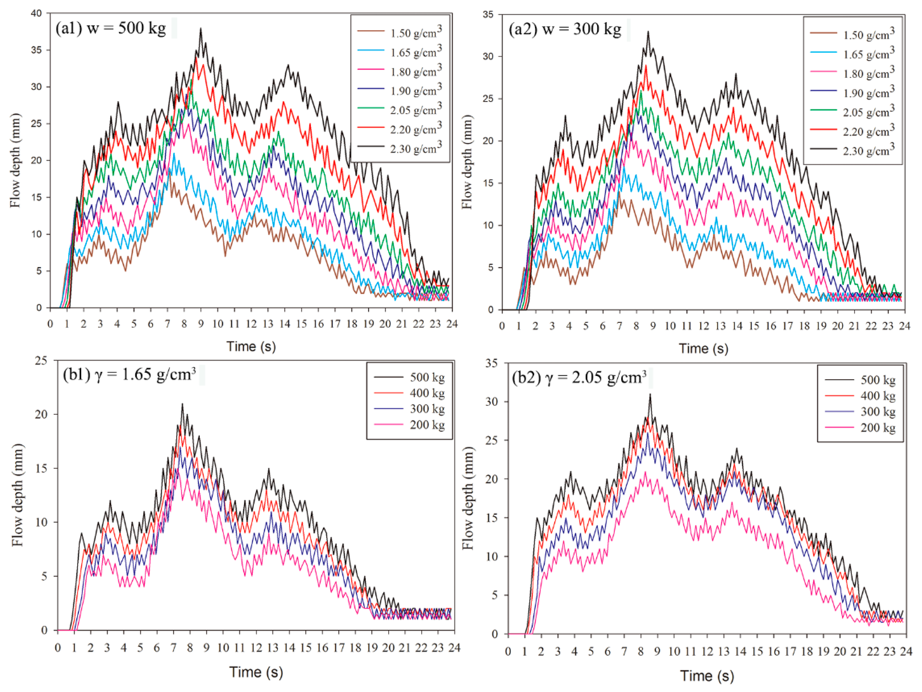
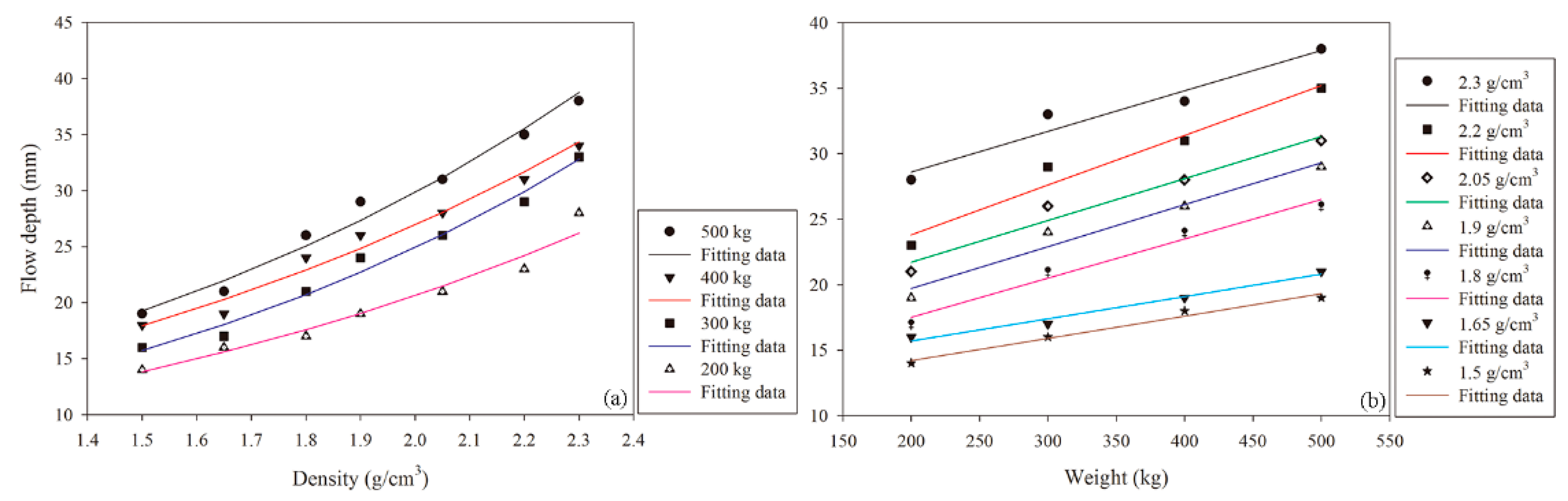
The flow depth was strongly correlated with the mixture density and the total weight for all combinations of these parameters, and the flow depths increased with increasing density (Figure 5). The inertial force was greater than the gravitational force for the low-density mixtures, so the depth remained relatively small; however, the viscosity force increased with increasing density, so the depth gradually increased [58]. In addition, the maximum flow depth increased with increasing density for a given flow weight, indicating a strong relationship between the density and flow depth. The maximum flow depth increased to as much as 2 times the minimum depth as the density increased from 1.5 g/cm3 to 2.3 g/cm3. The flow depths increased to approximately 1.3 times and 1.5 times the minimum depth when the density increased from 1.5 g/cm3 to 1.8 g/cm3 and from 1.8 to 2.3 g/cm3, respectively.
For a given mixture density, the flow depth changed greatly when the weight ranged from 500 kg to 200 kg, especially at high density, which indicates that the peak discharge is influenced by the weight (thus, the volume) of the flow (Figure 5b). As the weight of the mixture decreased over time, the inertial force also decreased and the flow depth decreased [67].
3.3. Flow Velocity
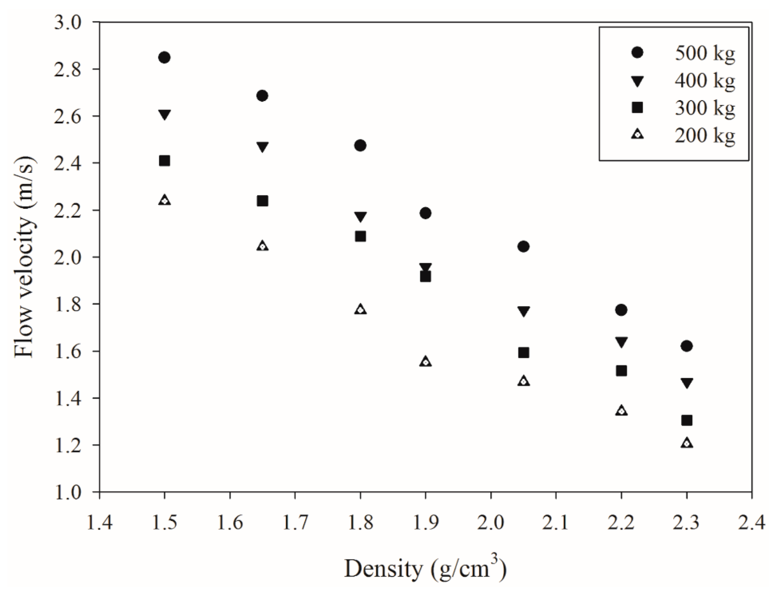
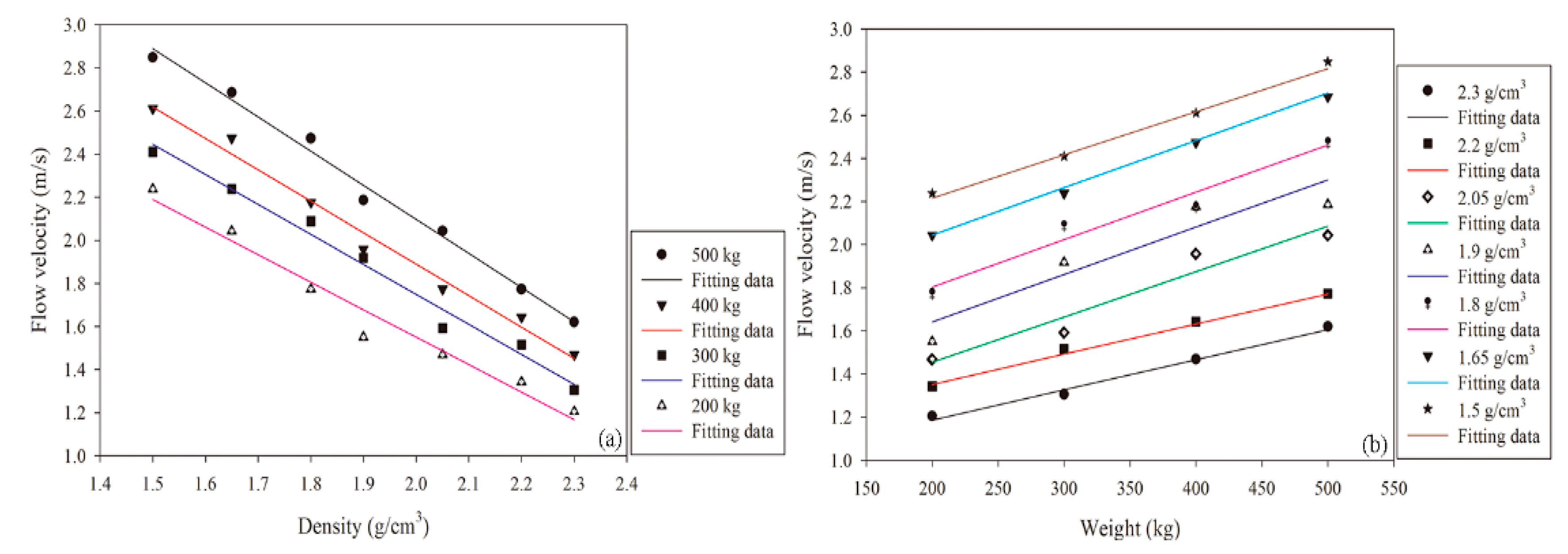
We found that the mean frontal flow velocity was strongly correlated with the mixture density and the total weight (Figure 6). The velocity gradually decreased with increasing density for a given mixture weight and with decreasing mixture weight for a given density. The flow velocity decreased below about 1.8 m/s as the mixture density increased from 1.5 g/cm3 to 2.3 g/cm3. The flow velocity also decreased by approximately 1.2 times and 1.5 times as the density increased from 1.5 g/cm3 to 1.8 g/cm3 and from 1.8 g/cm3 to 2.3 g/cm3, respectively. This indicated that low-density debris flow fastest, and that the high-density debris flowed slowly. When the mixture weight decreased from 500 kg to 400 kg, the flow velocity decreased by about 8%. Because of the inertial force increased with increasing mixture weight, it gradually increased for a given mixture density [67]. Our results therefore confirm the results of previous studies, which reported that debris flow density and mixture weight both strongly affected the debris flow velocity [5,38,72]. Combined with the flow depth analysis, these results let us calculate the impact force of the flowing debris.
3.4. Stress and Pressure Measurements
3.4.1. Total Normal Stress
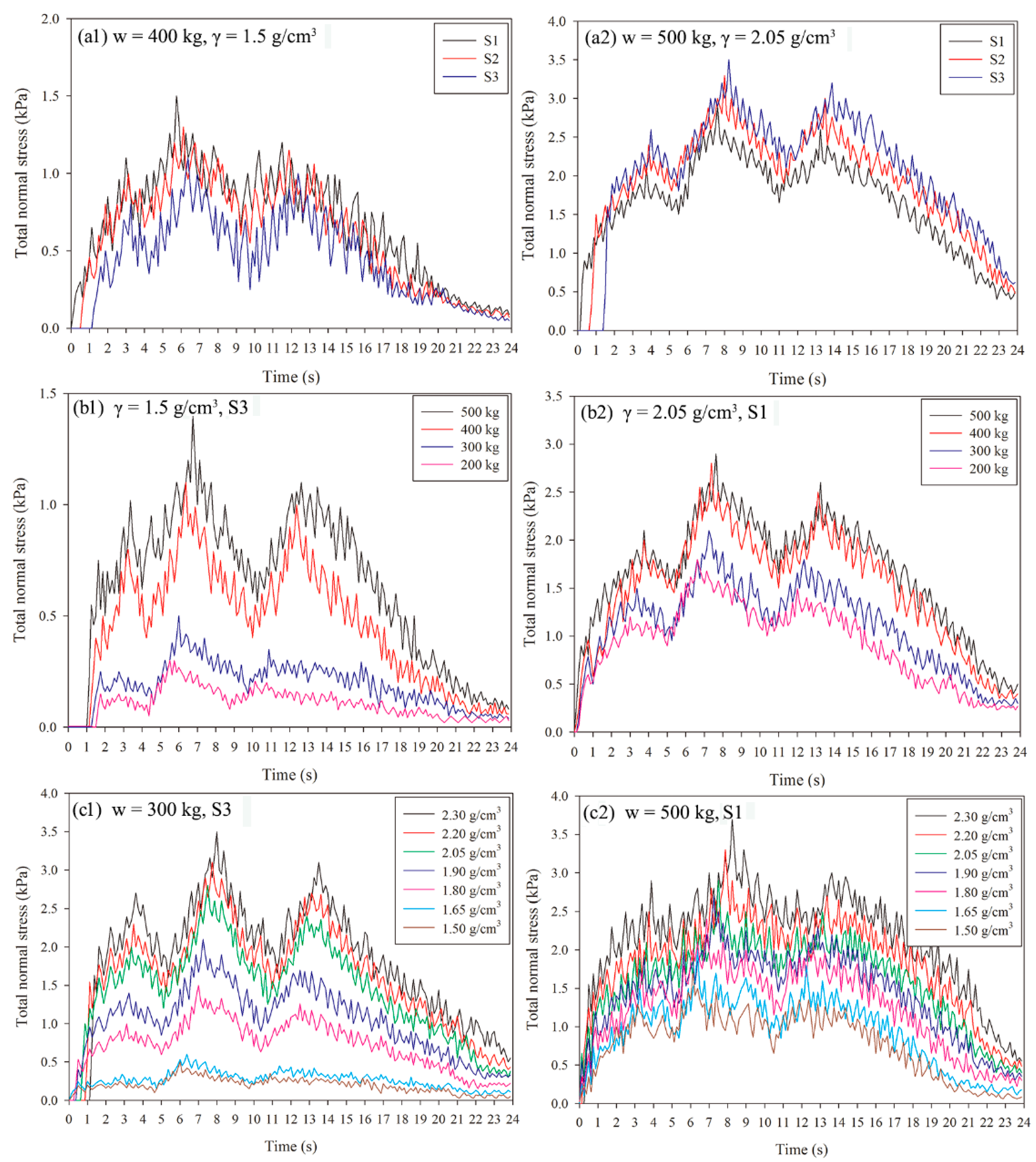
The temporal evolution of the total normal stress at the base of the debris flow was similar at the three monitoring points that we used to compare the effects of different mixture densities and weights (Figure 7). The maximum total normal stress values were observed at position S3 when the density was larger mixtures. However, the maximum stress mainly occurred at position S2 when the density was 1.8 or 1.9 g/cm3, and at position S1 when the density was low (i.e., 1.5 or 1.65 g/cm3). These results illustrate that the maximum values moved upstream as the mixture density decreased (Figure 7a). For a given density and monitoring point, the peak total normal stress increased with increasing weight, and the peak position gradually occurred later (Figure 7b). The magnitude of this change increased as the weight of the mixture increased from 200 kg to 500 kg. An especially large difference in the stress was observed when the weight increased from 300 kg to 400 kg.
These results indicate that the normal stress was influenced by the mixture weight. The peak occurred farther upstream when the mixture density decreased at a given measuring point for a given weight. During the experiments, the total normal stress increased most when the density increased from 1.65 g/cm3 to 1.8 g/cm3. Therefore, there were obvious changes in the total normal stress as the mixture density increased (Figure 7c). The changes with respect to density result from the increasing proportion of the weight accounted for by water as the mixture density decreased, since the water decreased the resistance to flow, resulting in a faster flow velocity and reduced total normal stress [75]. However, the results differed for the high-density debris flow; although the weight of the mixture (thus, the gravitational force) was higher due to the higher content of particles, the resistance to flow also increased due to the decreased water content.
At a given mixture weight, the total normal stress gradually increased with increasing density at all three monitoring positions. To better ascertain the maximum peaks under different combinations of mixture density and weight, we calculated the average value for the three monitoring points. The peak total normal stress increased to between 2.5 and 2.8 times the initial value as the mixture density increased from 1.5 g/cm3 to 2.3 g/cm3. The stress also increased to between 1.5 and 3 times the initial value when the density increased from 1.5 g/cm3 to 1.8 g/cm3, versus approximately 1.8 times as the density increased from 1.8 g/cm3 to 2.3 g/cm3. Thus, the total normal stress was strongly influenced by the mixture density. In addition, as the mixture weight increased from 200 kg to 500 kg at a given density, the stress increased to approximately 6 times the initial value. However, the change was largest when the weight increased from 300 kg to 400 kg.
3.4.2. Pore Fluid Pressure
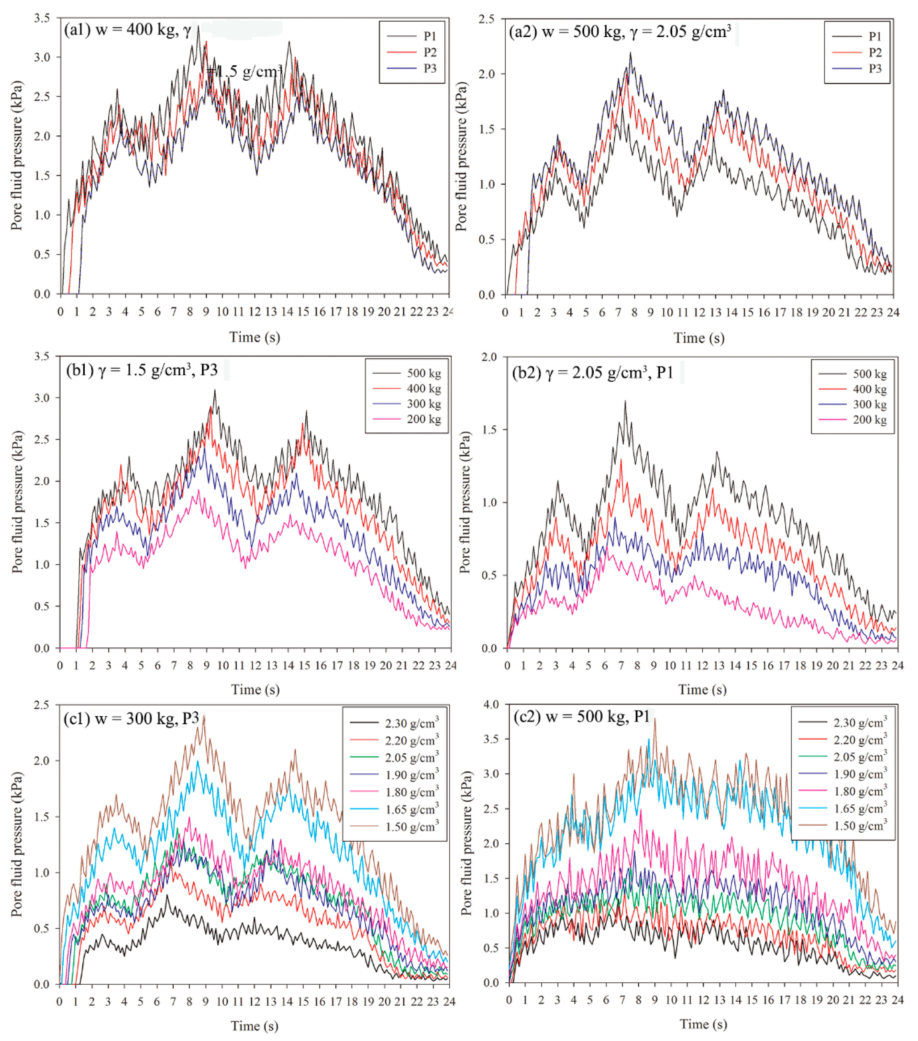
The temporal evolution of the pore fluid pressure showed a pattern (Figure 8) similar to that of the total normal stress. The peak also occurred later when the sensors were located upstream, midstream and downstream in the flume for a given mixture density and weight (Figure 8a). The maximum values were mainly distributed downstream when the density was highest; however, they were located midstream when the density was 1.8 g/cm3 or 1.9 g/cm3. The maximum peak was upstream when the mixture had a density <1.8 g/cm3. These results illustrate that the maximum values shift from the top of the flume to the bottom as the mixture density decreases (Figure 8a). The peak became increasingly large as the mixture weight increased at a given density and measurement position, and the position of the peak occurred later in the flow (Figure 8b). The magnitude of change changed greatly as the weight of the mixture increased from 200 kg to 500 kg. The magnitude of increase was largest when the mixture weight increased from 200 kg to 300 kg. For a given mixture weight and monitoring position, the peak occurred later as the mixture density decreased. The magnitude of the decrease was largest when the density increased from 1.65 g/cm3 to 1.8 g/cm3. These results indicate that the pore fluid pressure changed greatly as the density changed (Figure 8c). In addition, a low-density debris flow sustains high pore fluid pressure during the flow, thus increasing the mobility of the debris and increasing the likelihood that the debris will be liquefied [76], and our results agree with previous experimental results [6]. However, for the high-density debris flow, we found reduced mobility of the debris and a reduced likelihood that the debris will liquefy.
The pore fluid pressure at each measurement point gradually decreased with increasing density for a given mixture weight. To simplify the discussion, we again chose the mean value for the three measurement points. The mean increased by approximately 2.5 to 6 times as the density decreased from 2.3 g/cm3 to 1.4 g/cm3. The magnitude of the pore fluid pressure increased by 2 to 4 times with the density was high. However, when the density ranged from 1.8 g/cm3 to 1.5 g/cm3, the pore fluid pressure increased by only approximately 1.5 times. For a given mixture density, the increase in pore fluid pressure at 500 kg was to approximately 6 times the value with a mixture weight of 200 kg.
3.5. Development of Predictive Functions Based on the Study Data
Our study provided data on the flow depth, total normal stress, and pore fluid pressure as a function of the mixture weight and density. Because of the many combinations of values for these parameters, understanding their relationships is difficult, making it difficult to apply our results to engineering design applications to prevent or mitigate debris flows. To make this task easier, we developed predictive functions by fitting of the experimental results using version 9.1 of the DataFit software (New York, NY, USA, http://www.oakdaleengr.com/) and version 2015a of the MATLAB software (Beijing, China, https://www.mathworks.com/). The resulting equations make it easier to understand the relationships among the kinematics parameters and account for them in engineering designs.
Figure 9 presents the maximum flow depth as a function of the mixture weight and density, for which we found the best fits for exponential and linear relationships. Figure 10 shows linear relationships between the maximum flow velocity and the mixture weight and density. Figure 11 shows the relationship between the maximum total normal stress and the mixture weight and density, and Figure 12 shows the relationship between the maximum pore fluid pressure and the mixture weight and density. The functions for the pore fluid pressure and total normal stress a function of the mixture was linear, whereas those for the mixture density were logarithmic.
3.5.1. Parameterization of the Fitting Functions
Using the data in Figure 9, Figure 10, Figure 11 and Figure 12, we calculated regression equations for each of the relationships shown in those figures. We used the following equations:
where D is the maximum flow depth, S is the maximum total normal stress, V is the mean flow velocity, P is the maximum pore fluid pressure, γ is the density, and w is the mixture weight. The other variables are regression coefficients.
D = f(γ, w) = (aw + b) × (c × edγ)
V = f(γ, w) = (uw + k) × (yγ + z)
S = f(γ, w) = (sgm + sh) × sSi × lnγ + sj)
P = f(γ, w) = (plm + pn) × (p0 × lnγ + pq),
3.5.2. Parameterized Functions
We used 28 groups of experimental data (i.e., combinations of mixture weights and densities) to determine the coefficients of Equations (17)–(20) by means of least-squares regression. Table 1, Table 2, Table 3 and Table 4 present these coefficients. Figure 13 and Figure 14 show the resulting response surfaces for these functions. We used the adjusted coefficient of determination (R2) to evaluate the fitting accuracy [77,78]. The results were all excellent, with an adjusted R2 value >0.93. Thus, our functions did a good job of explaining the variation in flow depth, flow velocity, total normal stress, and pore fluid pressure as a function of the mixture density and weight, which agrees with previous results [58,67,75].
4. Conclusions
We confirmed our study hypothesis that the four key parameters of debris flows that we studied (flow depth, flow velocity, total normal pressure, and pore fluid pressure) were strongly and significantly related to the weight and density of each debris flow mixture. Debris flows that involve loess material cause large amounts of damage in China and elsewhere in the world. Our results provide an improved understanding of the kinematics of the debris flow processes. The resulting parameterized equations can be used by engineers to develop improved structures to prevent or mitigate damage from these flows.
We found that the flow velocity decreases with increasing mixture density but that the maximum discharge at the accumulation plate increased with increasing density. We developed hydrographs for each combination of weight and density that revealed four stages in the flow regime. Understanding these patterns may provide additional insights into the development of effective flow-control structures. The flow depth increased with increasing mixture density, and the magnitude of the increase was greatest at the highest densities. The flow velocity decreased with increasing density for a given mixture weight. The impact pressure of a debris flow can now be predicted based on the flow depth and velocity. The magnitude of the total normal stress increased and the pore fluid pressure decreased with increasing mixture density. The magnitude of the increase in the total normal stress decreased with increasing density, whereas the opposite pattern existed for the pore fluid pressure. These results clearly demonstrate that the flow depth, flow velocity, total normal stress, and pore fluid pressure depended strongly on the mixture density and weight.
The parameterized equations we developed for the relationships among the parameters were highly accurate, and can therefore be used to generate predictions that will help engineers design more effective structures to prevent or mitigate debris flows.
There are several limitations to our study. We used only one slope angle for the flume. To account for real-world conditions, it will be necessary to repeat our study for a range of slope angles. In addition, our research apparatus included roughness elements in the accumulation plane, but did not account for the effects of uneven terrain or obstacles. It will therefore be necessary to develop a more realistic simulated terrain to analyze the effects of topographic variation on debris flows.
Author Contributions
The laboratory tests were mainly carried out by H.S. and H.Y., and supervised by J.M. All the authors contributed to the design, installation, while the data analysis was principally finished by H.S. and J.M., and H.S. wrote the paper and the other authors made contributions to the study and wrote the manuscript.
Funding
This research was funded by the National Key Technology R&D Program of China (No. 2011BAK12B05) and National Key R&D Program of China (ID:2018YFC1504803). The author, Heping Shu, wishes to express his gratitude to the Chinese Scholarship Council for financial support pursuing his visiting study at Polytechnic University of Catalonia.
Conflicts of Interest
The authors declare no conflict of interest.
References
- Hungr, O.; Evans, S.; Bovis, M.; Hutchinson, J. A review of the classification of landslides of the flow type. Environ. Eng. Geosci. 2001, 7, 221–238. [Google Scholar] [CrossRef]
- Godt, J.W.; Coe, J.A. Alpine debris-flows triggered by a 28 July 1999 thunderstorm in the Central Front Range, Colorado. Geomorphology 2007, 84, 80–97. [Google Scholar] [CrossRef]
- Pudasaini, S.P. A general two-phase debris flow model. J. Geophys. Res. 2012, 117. [Google Scholar] [CrossRef] [Green Version]
- Takahashi, T. Debris Flow: Mechanics, Prediction and Counter-Measures, 2nd ed.; CRC Press: Boca Raton, FL, USA, 2014; p. 574. [Google Scholar]
- Wang, F.; Chen, X.Q.; Chen, J.G.; You, Y. Experimental study on a debris-flow drainage channel with different types of energy dissipation baffle. Eng. Geol. 2017, 220, 43–51. [Google Scholar] [CrossRef]
- Iverson, R.M. The physics of debris flows. Rev. Geophys. 1997, 35, 245–296. [Google Scholar] [CrossRef] [Green Version]
- Iverson, R.M.; Reid, M.E.; Logan, M.; Lahusen, R.G.; Godt, I.W.; Groswold, J.P. Positive feedback and momentum growth during debris-flow entrainment of wet bed sediment. Nat. Geosci. 2011, 4, 116–121. [Google Scholar] [CrossRef]
- VanDine, D.F.; Bovis, M. History and goals of Canadian debris-flow research. Nat. Hazards 2002, 26, 67–80. [Google Scholar] [CrossRef]
- Tang, C.; Zhu, J.; Li, W.L.; Liang, J.T. Rainfall-triggered debris flows following the Wenchuan earthquake. Bull. Eng. Geol. Environ. 2009, 68, 187–194. [Google Scholar] [CrossRef]
- Xu, Q.; Zhang, S.; Li, W.L.; van Asch, T.W.J. The 13 August 2010 catastrophic debris flows after the 2008 Wenchuan earthquake, China. Nat. Hazards Earth Syst. Sci. 2012, 12, 201–216. [Google Scholar] [CrossRef] [Green Version]
- Cui, P.; Zhou, G.G.D.; Zhu, X.H.; Zhang, J.Q. Scale amplification of natural debris flows caused by cascading landslide dam failures. Geomorphology 2013, 182, 173–189. [Google Scholar] [CrossRef]
- Han, Z.; Wang, W.D.; Li, Y.G.; Huang, J.L.; Su, B.; Tang, C.; Chen, G.Q.; Qu, X. An integrated method for rapid estimation of the valley incision by debris flows. Eng. Geol. 2018, 232, 34–35. [Google Scholar] [CrossRef]
- Jakob, M.; Friele, P. Frequency and magnitude of debris flows on Cheekye River, British Columbia. Geomorphology 2010, 114, 382–395. [Google Scholar] [CrossRef]
- Stoffel, M.; Mendlik, T.; Schneuwly-Bollschweiler, M.; Gobiet, A. Possible impacts of climate change on debris-flow activity in the Swiss Alps. Clim. Chang. 2014, 122, 141–155. [Google Scholar] [CrossRef]
- Li, Y.; Ma, C.; Wang, Y. Landslides and debris flows caused by an extreme rainstorm on 21 July 2012 in mountains near Beijing, China. Bull. Eng. Geol. Environ. 2017, 1–16. [Google Scholar] [CrossRef]
- Lyu, H.M.; Shen, J.S.; Arulrajah, A. Assessment of geohazards and preventative countermeasures using AHP incorporated with GIS in Lanzhou, China. Sustainability 2018, 10, 304. [Google Scholar] [CrossRef]
- Jakob, M. Debris-Flow Hazard Analysis. In Debris-Flow Hazards and Related Phenomena; Jakob, M., Hungr, O., Eds.; Springer: Berlin, Germany, 2005; pp. 411–443. [Google Scholar]
- Hürlimann, M.; Copons, R.; Altimir, J. Detailed debris flow hazard assessment in Andorra: A multidisciplinary approach. Geomorphology 2006, 78, 359–372. [Google Scholar] [CrossRef]
- Cavalli, M.; Marchi, L. Characterisation of the surface morphology of an alpine alluvial fan using airborne LiDAR. Nat. Hazards Earth Syst. Sci. 2008, 8, 323–333. [Google Scholar] [CrossRef] [Green Version]
- Jeong, S.; Kim, Y.; Lee, J.K.; Kim, J. The 27 July 2011 debris flows at Umyeonsan, Seoul, Korea. Landslides 2015, 12, 799–813. [Google Scholar] [CrossRef]
- Bai, S.; Xu, Q.; Wang, J.; Zhou, P. Pre-conditioning factors and susceptibility assessments of Wenchuan earthquake landslide at the Zhouqu segment of Bailongjiang basin, China. J. Geol. Soc. India 2013, 82, 575–582. [Google Scholar] [CrossRef]
- Fan, X.; Xu, Q.; Scaringi, G.; Li, S.; Peng, D. A chemo-mechanical insight into the failure mechanism of frequently occurred landslides in the Loess Plateau, Gansu Province, China. Eng. Geol. 2016, 228, 337–345. [Google Scholar] [CrossRef]
- Yuan, B.; Chen, W.W.; Tang, Y.Q.; Li, J.P.; Yang, Q. Experimental study on gully-shaped mud flow in the loess area. Environ. Earth Sci. 2015, 74, 759–769. [Google Scholar] [CrossRef]
- Derbyshire, E. Geological hazards in loess terrain, with particular reference to the loess regions of China. Earth Sci. Rev. 2001, 54, 231–260. [Google Scholar] [CrossRef]
- Cui, P.; Zeng, C.; Lei, Y. Experimental analysis on the impact force of viscous debris flow. Earth Surf. Process. Landf. 2015, 40, 1644–1655. [Google Scholar] [CrossRef] [Green Version]
- Chen, J.G.; Chen, X.Q.; Li, Y.; Wang, F. An experimental study of dilute debris flow characteristics in a drainage channel with an energy dissipation structure. Eng. Geol. 2015, 193, 224–230. [Google Scholar] [CrossRef]
- Hubl, J.; Suda, J.; Proske, D.; Kaitna, R.; Scheidl, C. Debris flow impact estimation. In Proceedings of the 11th International Symposium on Water Management and Hydraulic Engineering, Ohrid, Macedonia, 8–12 September 2009; Volume 1, pp. 137–148. [Google Scholar]
- Armanini, A.; Larcher, M. Rational criterion for designing opening of slit-check dam. J. Hydraul. Eng. 2001, 127, 94–104. [Google Scholar] [CrossRef]
- Huebl, J.; Fiebiger, G. Debris-Flow Mitigation Measures. In Debris-Flow Hazards and Related Phenomena; Jakob, M., Hungr, O., Eds.; Springer: Berlin, Germany, 2005; pp. 445–466. [Google Scholar]
- Hassanli, A.M.; Nameghi, A.E.; Beecham, S. Evaluation of the effect of porous check dam location on fine sediment retention (a case study). Environ. Monit. Assess. 2009, 152, 319–326. [Google Scholar] [CrossRef] [PubMed]
- Takahisa, M. Structural countermeasures for debris flow disasters. Int. J. Eros. Control Eng. 2008, 1, 8–43. [Google Scholar] [CrossRef]
- You, Y.; Pan, H.L.; Liu, J.F.; Ou, G.Q. The optimal cross-section design of the “Trapezoid-V” shaped drainage channel of viscous debris flow. J. Mt. Sci. 2011, 8, 103–107. [Google Scholar] [CrossRef]
- Wendeler, C.; McArdell, B.; Volkwein, A.; Denk, M.; Gröner, E. Debris flow mitigation with flexible ring net barriers—Field tests and case studies. WIT Trans. Eng. Sci. 2008, 60, 23–31. [Google Scholar] [CrossRef]
- Volkwein, A.; Baumann, R.; Rickli, C.; Wendeler, C. Standardization for Flexible Debris Retention Barriers; Lollino, G., Giordan, D., Crosta, G.B., Corominas, J., Azzam, R., Wasowski, J., Sciarra, N., Eds.; Springer: Berlin, Germany, 2011; Volume 2, pp. 193–196. [Google Scholar]
- Liu, J.F.; Nakatani, K.; Mizuyama, T. Effect assessment of debris flow mitigation works based on numerical simulation by using Kanako 2D. Landslides 2013, 10, 161–173. [Google Scholar] [CrossRef]
- Okano, K.; Suwa, H.; Kanno, T. Characterization of debris flows by rainstorm condition at a torrent on the Mount Yakedake volcano, Japan. Geomorphology 2012, 136, 88–94. [Google Scholar] [CrossRef]
- Navratil, O.; Liébault, F.; Bellot, H.; Travaglini, E.; Theule, J.; Chambon, G.; Laigle, D. High-frequency monitoring of debris-flow propagation along the Réal Torrent, Southern French Prealps. Geomorphology 2013, 201, 157–171. [Google Scholar] [CrossRef]
- Rickenmann, D. Empirical relationships for debris flows. Nat. Hazards 1999, 19, 47–77. [Google Scholar] [CrossRef]
- Song, E.; Sang, J.I.; Dongyeob, K.D.; Kun, W.C. Flow and deposition characteristics of sediment mixture in debris flow flume experiments. For. Sci. Technol. 2017, 13, 61–65. [Google Scholar] [CrossRef]
- Suwa, H.; Okud, S.; Yokoya, K. Observation system on rocky mud-flow. Bull. Dis. Prev. Res. Inst. 1973, 23, 59–73. [Google Scholar]
- Hu, K.H.; Wei, F.Q.; Li, Y. Real-time measurement and preliminary analysis of debris-flow impact force at Jiangjia Ravine, China. Earth Surf. Process. Landf. 2011, 36, 1268–1278. [Google Scholar] [CrossRef]
- Wendeler, C.; Volkwein, A.; Roth, A.; Denk, M.; Wartmann, S. Field Measurements Used for Numerical Modelling of Flexible Debris Flow Barriers. In Debris-Flow Hazards Mitigation, Mechanics, Prediction, and Assessment; Chen, C.I., Major, J.J., Eds.; Millpress: Rotterdam, The Netherlands, 2007; pp. 681–687. [Google Scholar]
- Hürlimann, M.; Abancó, C.; Moya, J.; Vilajosana, I. Results and experiences gathered at the Rebaixader debris-flow monitoring site, Central Pyrenees, Spain. Landslides 2013, 11, 939–953. [Google Scholar] [CrossRef]
- Morino, C.; Conway, S.J.; Balme, M.R.; Hillier, J.; Jordan, C.; Saemundsson, Þ.; Argles, T. Debris-flow release processes investigated through the analysis of multi-temporal LiDAR datasets in north-western Iceland. Earth Surf. Process. Landf. 2018. [Google Scholar] [CrossRef]
- Bossi, G.; Cavalli, M.; Crema, S.; Frigerio, S.; Quan Luna, B.; Mantovani, M.; Marcato, G.; Schenato, L.; Pasuto, A. Multi-temporal LiDAR-DTMs as a tool for modelling a complex landslide: A case study in the Rotolon catchment (eastern Italian Alps). Nat. Hazards Earth Syst. Sci. 2015, 15, 715–722. [Google Scholar] [CrossRef]
- Cavalli, M.; Goldin, B.; Comiti, F.; Brardinoni, F.; Marchi, L. Assessment of erosion and deposition in steep mountain basins by differencing sequential digital terrain models. Geomorphology 2017, 291, 4–16. [Google Scholar] [CrossRef]
- D’Agostino, V.; Cesca, M.; Marchi, L. Field and laboratory investigations of runout distances of debris flows in the Dolomites (Eastern Italian Alps). Geomorphology 2010, 115, 294–304. [Google Scholar] [CrossRef]
- Scheidl, C.; Chiari, M.; Kaitna, R.; Müllegger, M.; Krawtschuk, A.; Zimmermann, T.; Proske, D. Analysing debris-flow impact models, based on a small scale modelling approach. Surv. Geophys. 2013, 34, 21–140. [Google Scholar] [CrossRef]
- Haas, T.; Braat, L.; Leuven, J.R.F.W.; Lokhorst, I.R.; Kleinhans, M.G. Effects of debris flow composition on runout, depositional mechanisms, and deposit morphology in laboratory experiments. J. Geophys. Res. Earth Surf. 2015, 120, 1949–1972. [Google Scholar] [CrossRef] [Green Version]
- Hürlimann, M.; Rickenmann, D.; Graf, C. Field and monitoring data of debris-flow events in the Swiss Alps. Can. Geotech. J. 2003, 40, 161–175. [Google Scholar] [CrossRef]
- Takahashi, T. A review of Japanese debris flow research. Int. J. Eros. Control Eng. 2009, 2, 1–14. [Google Scholar] [CrossRef]
- McCoy, S.W.; Kean, J.W.; Coe, J.A.; Staley, D.M.; Wasklewicz, T.A.; Tucker, G.E. Evolution of a natural debris flow: In situ measurements of flow dynamics, video imagery, and terrestrial laser scanning. Geology 2010, 38, 735–738. [Google Scholar] [CrossRef]
- Marchi, L.; Tecca, P.R. Dating Torrential Processes on Fans and Cones. In Debris-Flow Monitoring in Italy; Schneuwly-Bollschweiler, M., Stoffel, M., Rudolf-Miklau, F., Eds.; Springer: Berlin, Germany, 2013; pp. 309–318. [Google Scholar]
- Moriguchi, S.; Borja, R.; Yashima, A.; Sawada, K. Estimating the impact force generated by granular flow on a rigid obstruction. Acta Geotech. 2009, 4, 57–71. [Google Scholar] [CrossRef]
- Iverson, R.M. Scaling and design of landslide and debris-flow experiments. Geomorphology 2015, 244, 9–20. [Google Scholar] [CrossRef]
- Arattano, M.; Franzi, L. On the evaluation of debris flows dynamics by means of mathematical models. Nat. Hazards Earth Syst. Sci. 2003, 3, 539–544. [Google Scholar] [CrossRef] [Green Version]
- Armanini, A.; Larcher, M.; Odorizzi, M. Dynamic impact of a debris flow front against a vertical wall. In Proceedings of the 5th International Conference on Debris-flow Hazard Mitigation, Rome, Italy, 14–17 June 2011; Genevois, R., Douglas, L., Eds.; Casa Editrice Università La Sapienza: Roma, Italy, 2011; pp. 1041–1049. [Google Scholar]
- Wang, D.; Chen, Z.; He, S.; Liu, Y.; Tang, H. Measuring and estimating the impact pressure of debris flows on bridge piers based on large-scale laboratory experiments. Landslides 2018, 15, 1331–1345. [Google Scholar] [CrossRef]
- Egashira, S.; Honda, N.; Itoh, T. Experimental study on the entrainment of bed material into debris flow. Phys. Chem. Earth Part C 2001, 26, 645–650. [Google Scholar] [CrossRef]
- Acharya, G.; Cochrane, T.; Davies, T.; Bowman, E. Quantifying and modeling postfailure sediment yields from laboratory-scale soil erosion and shallow landslide experiments with silty loess. Geomorphology 2011, 129, 49–58. [Google Scholar] [CrossRef]
- Peng, J.; Huo, A.; Cheng, Y.; Dang, J.; Wei, H.; Wang, X.; Li, C. Submersion simulation in a typical debris flow watershed of Jianzhuangchuan catchment, Loess Plateau. Environ. Earth Sci. 2017, 76. [Google Scholar] [CrossRef]
- Peng, J.; Fan, Z.; Wu, D.; Zhuang, J.; Dai, F.; Chen, W.; Zhao, C. Heavy rainfall triggered loess-mudstone landslide and subsequent debris flow in Tianshui, China. Eng. Geol. 2015, 186, 79–90. [Google Scholar] [CrossRef]
- Tu, X.B.; Kwong, A.K.L.; Dai, F.C.; Tham, L.G.; Min, H. Field monitoring of rainfall infiltration in a loess slope and analysis of failure mechanism of rainfall induced landslides. Eng. Geol. 2009, 105, 134–150. [Google Scholar] [CrossRef]
- Shi, J.S.; Wu, L.Z.; Wu, S.R.; Li, B.; Wang, T.; Xin, P. Analysis of the causes of large-scale loess landslides in Baoji, China. Geomorphology 2016, 264, 109–117. [Google Scholar] [CrossRef]
- Tan, Q.M. Dimensional Analysis: With Case Studies in Mechanics; Springer: Berlin, Germany, 2011. [Google Scholar]
- Vagnon, F.; Segalini, A. Debris flow impact estimation on a rigid barrier. Nat. Hazards Earth Syst. Sci. 2016, 16, 1–17. [Google Scholar] [CrossRef]
- Choi, C.E.; Ng, C.W.W.; Au-Yeung, S.C.H.; Goodwin, G.R. Froude characteristics of both dense granular and water flows in flume modelling. Landslides 2015, 12, 1197–1206. [Google Scholar] [CrossRef]
- Ditzler, C.; Scheffe, K.; Monger, H.C. Soil Survey Manua, Soil Science Division Staff; USDA Handbook 18; Government Printing Office: Washington, DC, USA, 2017.
- Zhang, D.X.; Wang, G.H. Study of the 1920 Haiyuan earthquake-induced landslides in loess (China). Eng. Geol. 2007, 94, 76–88. [Google Scholar] [CrossRef]
- Xu, L.; Dai, F.C.; Tham, L.G.; Tu, X.B.; Min, H.; Zhou, Y.F.; Wu, C.X.; Xu, K. Field testing of irrigation effects on the stability of a cliff edge in loess, North-west China. Eng. Geol. 2011, 120, 10–17. [Google Scholar] [CrossRef]
- Wang, G.H.; Zhang, D.X.; Furuya, G.; Yang, J. Pore-pressure generation and fluidization in a loess landslide triggered by the 1920 Haiyuan earthquake, China: A case study. Eng. Geol. 2014, 174, 36–45. [Google Scholar] [CrossRef] [Green Version]
- Chen, J.G.; Chen, X.Q.; Wang, T.; Zou, Y.H.; Zhong, W. Types and causes of debris flow damage to drainage channels in the Wenchuan earthquake area. J. Mt. Sci. 2014, 11, 1406–1419. [Google Scholar] [CrossRef]
- Gaál, L.; Szolgay, J.; Kohnová, S.; Hlavčová, K.; Parajka, J.; Viglione, A.; Merz, R.; Blöschl, G. Dependence between flood peaks and volumes: A case study on climate and hydrological controls. Hydrol. Sci. J. 2015, 60, 968–984. [Google Scholar] [CrossRef]
- Kean, J.W.; McCoy, S.W.; Tucker, G.E.; Staley, D.M.; Coe, J.A. Runoff-generated debris flows: Observations and modeling of surge initiation, magnitude, and frequency. J. Geophys. Res. Earth Surf. 2013, 118, 2190–2207. [Google Scholar] [CrossRef] [Green Version]
- Lyu, L.; Wang, Z.; Cui, P.; Xu, M. The role of bank erosion on the initiation and motion of gully debris flows. Geomorphology 2017, 285, 137–151. [Google Scholar] [CrossRef]
- Ilstad, T.; Marr, J.G.; Elverhøi, A.; Harbitz, C.B. Laboratory studies of subaqueous debris flows by measurements of pore-fluid pressure and total stress. Mar. Geol. 2004, 213, 403–414. [Google Scholar] [CrossRef]
- Gujarati, D.N. Basic Econometrics; Tata McGraw-Hill Education: New Yrok, NY, USA, 2009. [Google Scholar]
- Song, F.; Wang, H.; Jiang, M.J. Analytically-based simplified formulas for circular tunnels with two liners in viscoelastic rock under anisotropic initial stresses. Constr. Build. Mater. 2018, 175, 746–767. [Google Scholar] [CrossRef]
Figure 1.
Schematic diagram of the experimental apparatus. Total normal stress sensors (labeled “S”) and pore fluid-pressure sensors (labeled “P”) are installed at upstream (S1 and P1), midstream (S2 and P2), and downstream (S3 and P3) positions.
Figure 1.
Schematic diagram of the experimental apparatus. Total normal stress sensors (labeled “S”) and pore fluid-pressure sensors (labeled “P”) are installed at upstream (S1 and P1), midstream (S2 and P2), and downstream (S3 and P3) positions.

Figure 2.
Particle-size distribution of the loess samples used to create the debris flow material that was used during the experiments. The shaded area represents the previously reported distributions for other loess materials [23,64,69,70,71].

Figure 3.
Video frames from the debris flow experiments with densities of (a) 1650 kg/m3 and (b) 2050 kg/m3.
Figure 3.
Video frames from the debris flow experiments with densities of (a) 1650 kg/m3 and (b) 2050 kg/m3.

Figure 4.
Example of a representative set of experimental results for the normal stress, pore pressure, and flow depth for a sample with a density of γ = 2200 kg/m3 and a weight of w = 500 kg. Data are for sampling positions S2 and P2 in Figure 1.
Figure 4.
Example of a representative set of experimental results for the normal stress, pore pressure, and flow depth for a sample with a density of γ = 2200 kg/m3 and a weight of w = 500 kg. Data are for sampling positions S2 and P2 in Figure 1.

Figure 5.
Effect on flow depth of (a1,a2) mixture density (γ) for two representative weights and (b1,b2) total mixture weight (w) for two representative densities.
Figure 5.
Effect on flow depth of (a1,a2) mixture density (γ) for two representative weights and (b1,b2) total mixture weight (w) for two representative densities.

Figure 6.
Effect of mixture density and total weight on the mean frontal flow velocity.

Figure 7.
Effect of mixture density (γ) and total weight (w) on the total normal stress at monitoring points S1 to S3 in Figure 1: (a1,a2) hydrographs for mixtures with constant weight and density at the three monitoring points (whose positions are shown in Figure 1); (b1,b2) hydrographs for mixtures with different weights but constant density at the three monitoring points; and (c1,c2) hydrographs for mixtures with different densities but constant weight at the three monitoring points.

Figure 8.
Changes in the pore fluid pressure as a function of mixture density and weight: (a1,a2) hydrographs for mixtures at the three monitoring points P1 to P3 (Figure 1) but with constant weight and density; (b1,b2) hydrographs for mixtures with different weights but with constant density at a given monitoring point; and (c1,c2) hydrographs for mixtures with different densities but with constant weight at a given monitoring point.

Figure 9.
Fitting functions for the maximum flow depth as a function of the mixture weight and density.
Figure 9.
Fitting functions for the maximum flow depth as a function of the mixture weight and density.

Figure 10.
Fitting functions for the maximum flow velocity as a function of the mixture weight and density.
Figure 10.
Fitting functions for the maximum flow velocity as a function of the mixture weight and density.

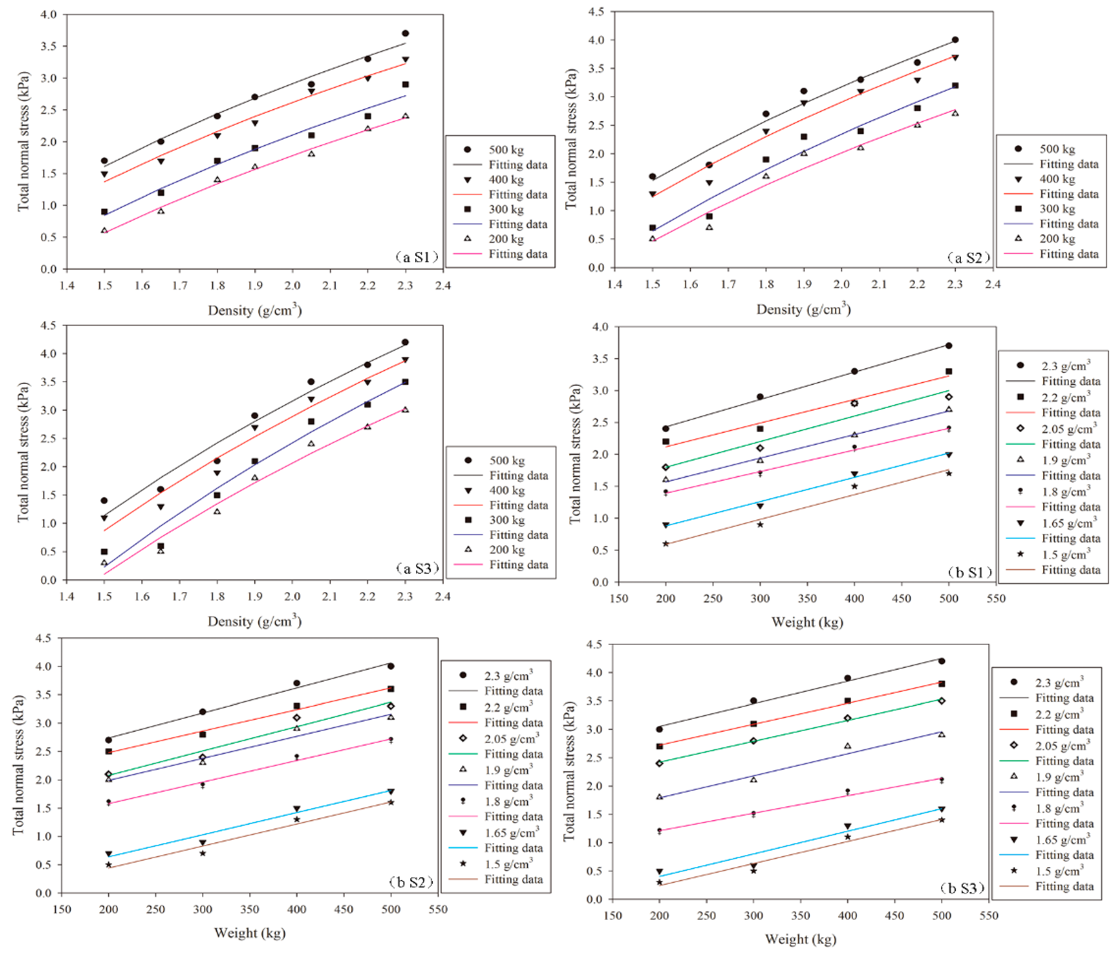
Figure 11.
Fitting function for the total normal stress: (a) the mixture weight and total normal stress; (b) the mixture density and total normal stress. The locations of positions S1 to S3 are shown in Figure 1.
Figure 11.
Fitting function for the total normal stress: (a) the mixture weight and total normal stress; (b) the mixture density and total normal stress. The locations of positions S1 to S3 are shown in Figure 1.

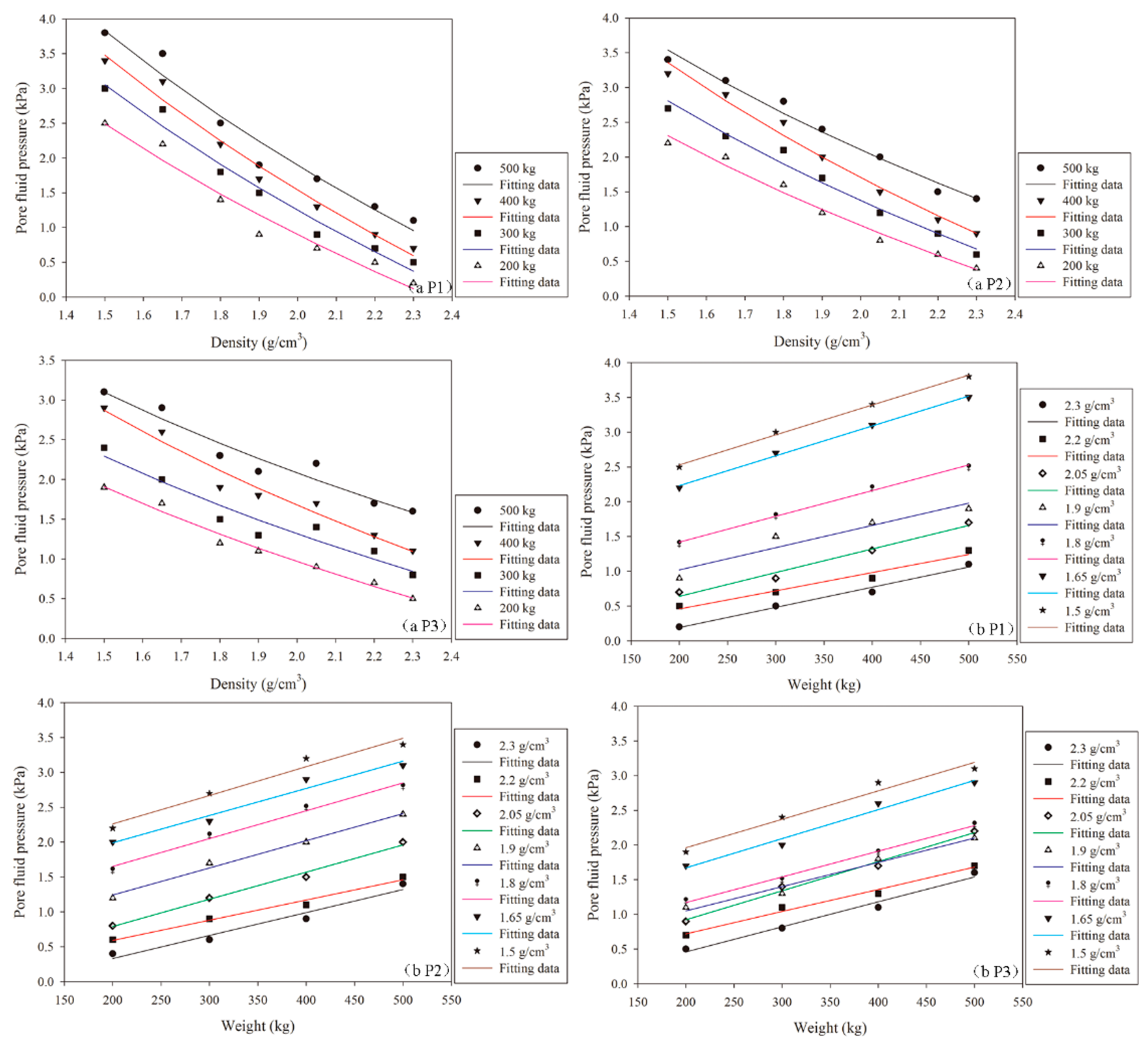
Figure 12.
Fitting function for the pore fluid pressure as a function of: (a) the mixture weight and pore fluid; (b) the mixture density and pore fluid pressure. The locations of positions P1 to P3 are shown in Figure 1.
Figure 12.
Fitting function for the pore fluid pressure as a function of: (a) the mixture weight and pore fluid; (b) the mixture density and pore fluid pressure. The locations of positions P1 to P3 are shown in Figure 1.

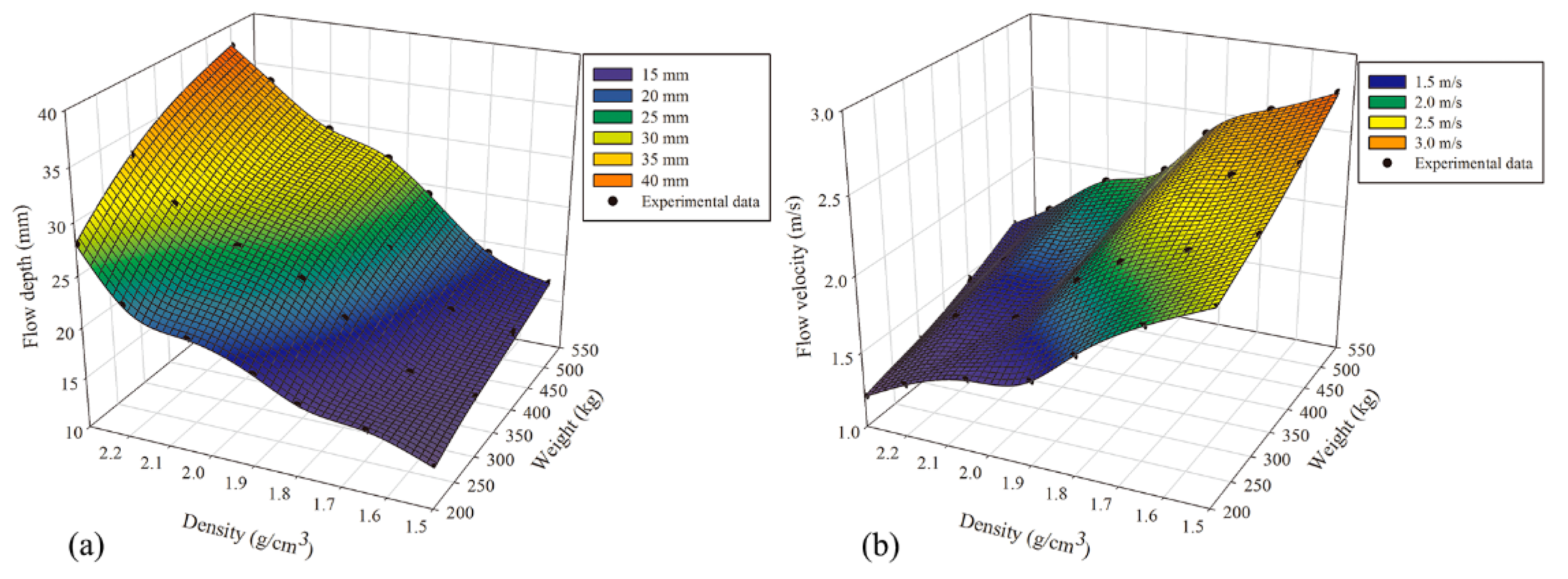
Figure 13.
Response surfaces for the (a) maximum flow depth, and (b) mean flow velocity as a function of mixture weight and density.
Figure 13.
Response surfaces for the (a) maximum flow depth, and (b) mean flow velocity as a function of mixture weight and density.

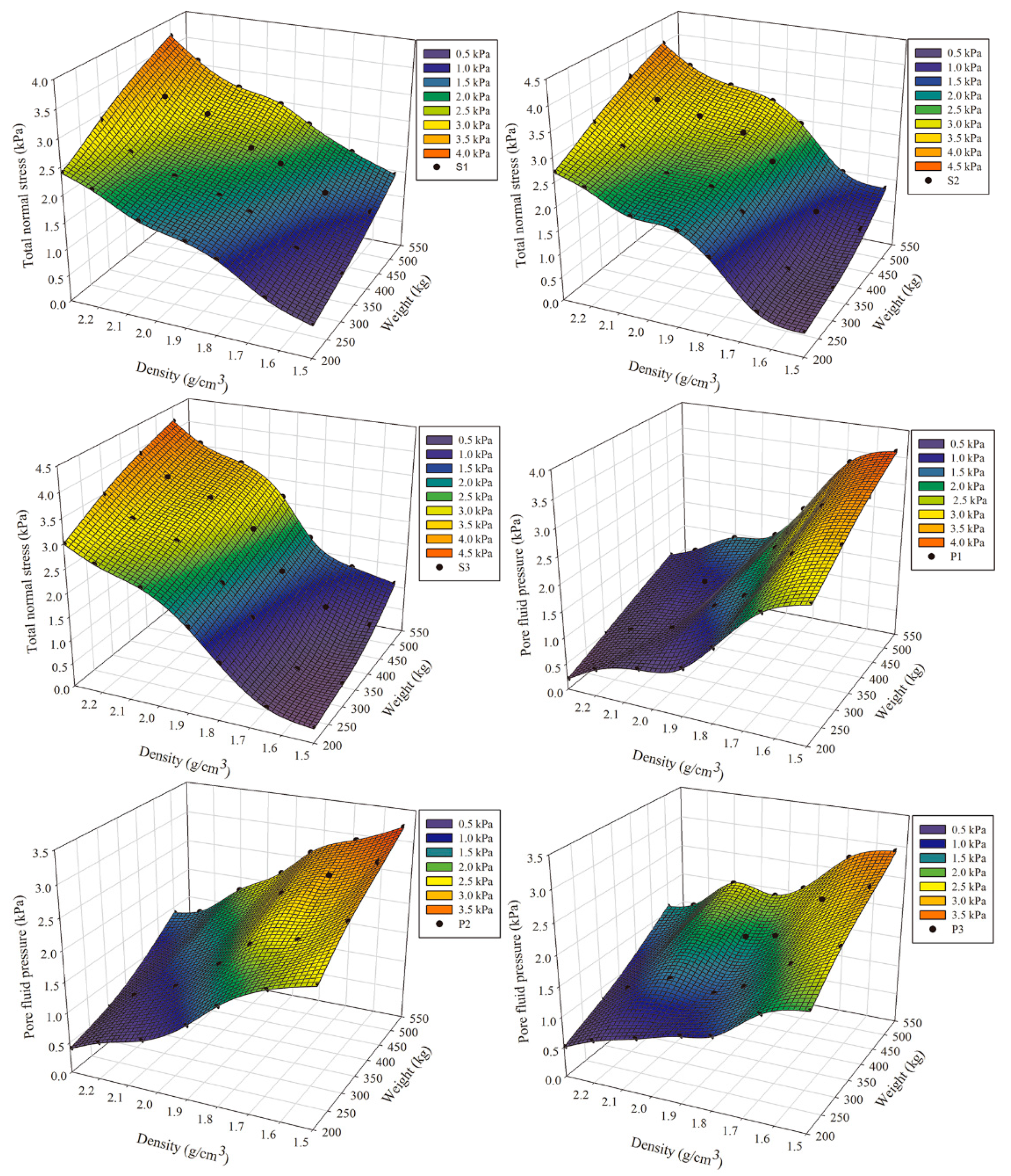
Figure 14.
Response surfaces for the maximum total normal stress at positions S1 to S3 (Figure 1) and maximum pore fluid pressure at positions P1 to P3 (Figure 1) as a function of mixture weight and density.


Table 1.
Coefficients in Equation (17) for maximum flow depth.
| Index | a | B | c | d | Adj. R2 |
|---|---|---|---|---|---|
| Coefficient value | 0.0524 | 27.2243 | 0.1044 | 0.8405 | 0.9729 |
Table 2.
Coefficients in Equation (18) for mean flow velocity.
| Index | u | K | y | z | Adj. R2 |
|---|---|---|---|---|---|
| Coefficient values | 0.0009 | 0.6280 | −1.5142 | 4.9659 | 0.9834 |
Table 3.
Coefficients in Equation (19) for maximum total normal stress at monitoring positions S1 to S3 (Figure 1).
Table 3.
Coefficients in Equation (19) for maximum total normal stress at monitoring positions S1 to S3 (Figure 1).
| Position | sg | sh | Si | si | Adj. R2 |
|---|---|---|---|---|---|
| S1 | 0.0022 | 0.5259 | 3.2798 | −0.4498 | 0.9603 |
| S2 | 0.0019 | 0.5764 | 4.3714 | −0.9746 | 0.9370 |
| S3 | 0.0016 | 0.6155 | 5.8129 | −1.8288 | 0.9412 |
Table 4.
Coefficients in Equation (20) for the maximum pore fluid pressure at monitoring positions P1 to P3 (Figure 1).
Table 4.
Coefficients in Equation (20) for the maximum pore fluid pressure at monitoring positions P1 to P3 (Figure 1).
| Position | pl | pn | po | pq | Adj. R2 |
|---|---|---|---|---|---|
| P1 | 0.0017 | 0.4085 | −6.0102 | 5.5407 | 0.9548 |
| P2 | 0.0019 | 0.3766 | −4.6781 | 4.7382 | 0.9586 |
| P3 | 0.0021 | 0.2782 | −3.3683 | 3.8258 | 0.9423 |
© 2018 by the authors. Licensee MDPI, Basel, Switzerland. This article is an open access article distributed under the terms and conditions of the Creative Commons Attribution (CC BY) license (http://creativecommons.org/licenses/by/4.0/).
Share and Cite
MDPI and ACS Style
Shu, H.; Ma, J.; Yu, H.; Hürlimann, M.; Zhang, P.; Liu, F.; Qi, S. Effect of Density and Total Weight on Flow Depth, Velocity, and Stresses in Loess Debris Flows. Water 2018, 10, 1784. https://doi.org/10.3390/w10121784
AMA Style
Shu H, Ma J, Yu H, Hürlimann M, Zhang P, Liu F, Qi S. Effect of Density and Total Weight on Flow Depth, Velocity, and Stresses in Loess Debris Flows. Water. 2018; 10(12):1784. https://doi.org/10.3390/w10121784
Chicago/Turabian StyleShu, Heping, Jinzhu Ma, Haichao Yu, Marcel Hürlimann, Peng Zhang, Fei Liu, and Shi Qi. 2018. "Effect of Density and Total Weight on Flow Depth, Velocity, and Stresses in Loess Debris Flows" Water 10, no. 12: 1784. https://doi.org/10.3390/w10121784
Note that from the first issue of 2016, this journal uses article numbers instead of page numbers. See further details here.