Real-Time Burst Detection in District Metering Areas in Water Distribution System Based on Patterns of Water Demand with Supervised Learning

Abstract

This paper proposes a new method to detect bursts in District Metering Areas (DMAs) in water distribution systems. The methodology is divided into three steps. Firstly, Dynamic Time Warping was applied to study the similarity of daily water demand, extract different patterns of water demand, and remove abnormal patterns. In the second stage, according to different water demand patterns, a supervised learning algorithm was adopted for burst detection, which established a leakage identification model for each period of time, respectively, using a sliding time window. Finally, the detection process was performed by calculating the abnormal probability of flow during a certain period by the model and identifying whether a burst occurred according to the set threshold. The method was validated on a case study involving a DMA with engineered pipe-burst events. The results obtained demonstrate that the proposed method can effectively detect bursts, with a low false-alarm rate and high accuracy.

1. Introduction

Water leakage in water distribution systems (WDS) is a common issue and has caused widespread concern in recent years [1]. One of the major forms of leakage are those caused by burst events (high volume and short duration). An underground burst in WDS may not be reported for a long time, resulting in a large amount of leakage [2]. Burst detection is a challenging problem that plagues water supply industries. Bursts will not only cause serious waste of water resources, but will also affect normal water supply [3]. For water supply industries, timely leakage detection in WDS is of great significance for ensuring the continuance of water supply, as well as public safety. For the purposes of improving burst detection efficiency, when trying to shorten the burst location detection time and evaluating the pipe network’s leakage level, water supply companies usually divide the entire pipe network into several small, separate district areas (district metering areas) for flow and pressure monitoring, as shown in Figure 1.

In the past few decades, with the development of supervisory control and data acquisition (SCADA) systems that can collect pressure and flow data in real time, data-driven methods have prevailed in leakage detection. There are generally three categories of data-driven methods: the classification method, prediction-classification method, and the statistical method. Most of these methods were tested and validated on DMA (district metering areas) under real circumstances [4]. Related studies about DMA burst detection primarily involve a single-inlet flow meter [5,6,7,8,9,10,11,12,13,14]. Mounce et al. (2002) presented a neural network methodology to detect bursts [5], and Mounce et al. (2006) proposed static and time-delay artificial neural networks (ANNs) to detect bursts. The results showed that the time-delay neural network was better than the static network [6]. Mounce et al. (2010) also combined mixture density (MDN) and fuzzy inference networks (FIS) to detect bursts [7]. Similarly, Romano et al. (2014) proposed a novel method to automatically detect bursts and other abnormal flow events in DMAs. The new methodology combined AI algorithm with the statistical process control (SPC) technique, as well as Bayesian inference systems [8]. Ye and Fenner (2011) proposed a method for burst detection by a Kalman filter (KF). This method requires a lot of normal historical dataset. By training a normal dataset, an optimal estimation for each time step is calculated, and the deviation between estimation and actual values represents the size of bursts. [9]. Besides, Ye and Fenner (2014) also proposed a methodology to use polynomial functions based on the weighted least squares method, with expectation maximization (EM) to predict normal flow or pressure values. When bursts occur in DMAs, observed data are significantly different from predictive values because predictions depend on normal historical data [10]. However, the above methods only determine whether or not burst occurs in DMA based on the predicted residual at a single time-point. When the predicted residual exceeds the set threshold, it indicates that a burst has occurred. In general, the choice of threshold should be based on the maximum prediction residual of the predictive model, but in practical applications, the choice of threshold often depends on experience, thus greatly limiting the detection effect of the threshold classification model. Besides, it is very easy for an outlier detection at one time-point to cause a false alarm, due to sudden water usage or a sensor fault. In addition, Jung and Lansey (2014) used the Kalman filter methodology to estimate the WDS state and detect bursts. To some extent, it avoided some false alarms caused by the operation of the pipe network [11]. Loureiro et al. (2016) introduced a renewed concept of outlier regions and utilized robust statistics to identify abnormal flow from DMAs [12].

Burst detection based on prediction classification or statistical methods mainly rely on lots of historical monitoring data under normal pipe conditions. Therefore, the method based on prediction classification should eliminate abnormal data included in historical data. According to the different manifestations of anomalies, time series anomalies can be mainly divided into point anomalies and pattern (sequence) anomalies, which are used to discover anomalies in a time series. In past research, in order to obtain the normal operating patterns dataset, it was widely used to determine the acceptable lower and upper confidence limits of each time point by statistical methods. If the value at a certain time point exceeded the defined upper or lower boundary, the data of the day needed to be removed. This data preprocessing method greatly reduces lots of normal historical data. In view of the fact that a pipe-burst is a sustained event, this paper studies pattern anomaly instead of point anomaly, which refers to the pattern that is significantly different from other patterns in time series. The pattern can characterize the main feature of time series and avoid the bad effects of some single-point outliers.

For real historical flow data, it is usually easy to obtain data that contain a large amount of normal data and a small amount of abnormal data. Thence, the primary question is how to distinguish those abnormal flow data from the normal ones. Secondly, most burst detection methods have better a detection effect on larger bursts than smaller ones. This is mainly because the flow data of DMAs are not fixed, and varies with time. Even at the same time of different days, the flow data will fluctuate within a certain normal range, and small bursts can easily be ignored. Aiming at solving the above problems, this paper proposes a methodology that uses supervised learning, with patterns of water demand to detect small bursts in DMAs.

2. Methodology

The method is mainly divided into three steps: (1) Firstly, using historical flow data of DMAs, the similarity of daily water demand is established, different patterns of water demand are extracted, and abnormal patterns are removed; (2) normal data is divided into different time-period segments using sliding windows, and burst events are added to normal flow data to simulate abnormal flow data (i.e., bursts). Then, the normal flow dataset (i.e., no bursts) and the abnormal flow dataset (bursts) can be trained by using the supervised learning algorithm, and the burst identification model can be established; (3) the detection process is performed by calculating the abnormal probability of flow during a certain period by the model, and identifying whether a burst occurs according to the defined threshold. The proposed method has been validated on a case study involving a DMA with engineered pipe-burst events (i.e., simulated by opening fire hydrants). Therefore, a diagrammatic representation of the burst identification process is shown in Figure 2.

2.1. Daily Patterns of Water Demand

As known already, time-series data change with time, yet appear to follow a certain regular pattern; however, there can be certain differences in different cycles. The data with the above characteristics is called pseudo-period data. Since the daily water consumption in the same area is almost the same, hydraulic data from water distribution systems is a type of pseudo-period data as well, as shown in Figure 3. Analysis of this type of data involves an important issue: how to find out abnormal patterns [15]. This paper presents the application of the Dynamic Time Warping (DTW) algorithm to study the similarity of patterns in such flow data. DTW was first used widely in the study of speech recognition. Berndt and Clifford (1994) put forward DTW into the study of time-series data [16]. Currently, DTW is being widely applied to many occasions involving time-series data. DTW is a method that calculates the minimum distance between two time series by bending the time axis, and determines the best correspondence between each point. Compared to Euclidean distance, DTW can solve the problem of stretching (or compressing) and linear drift along the time axis for two time-series data [17].

2.1.1. Dynamic Time Warping

The DTW algorithm is used to find the best-matching path between two time series by adjusting the correspondence between time points so as to measure the similarity of time series. Specifically, there are two kinds of time-series flow data: $da{y}_i=x_1,x_2,\cdots ,x_i,\cdots x_m$ and $da{y}_j=y_1,y_2,\cdots ,y_i,\cdots y_m$. The DTW distance $D(da{y}_i,da{y}_j)$ between $da{y}_i$ and $da{y}_j$ is defined as follows:

$$D(da{y}_i,da{y}_j)=d(m,m).$$

(1)

$$d(i,j)=dist(x_i,y_j)+\min [d(i,j-1),d(i-1,j),d(i-1,j-1)].$$

(2)

$$d(0,0)=0,d(i,0)=d(0,j)=\infty ,(i=1,2,\cdots ,m;j=1,2,\cdots ,m).$$

(3)

where $dist(x_i,y_j)$ can be calculated using different distance measurements (e.g., Euclidean distance, Manhattan distance, etc.). In this paper, let $dist(x_i,y_j)=\left|x_i-y_j\right|$.

When calculating the DTW distance between the time series $da{y}_i$ and $da{y}_j$, the algorithm needs to construct a dynamic time-warping distance matrix with $m\times m$, and the calculation process uses the recursive Formulation (2) to fill in the matrix. Since the calculation does not need to use the information of the whole matrix, the algorithm only needs to save the unit of the current column and the unit of the previous column in the matrix involved in the calculation. An example is shown in Figure 4.

2.1.2. Abnormal Daily Patterns of Water Demand

A method which can be used for detecting abnormal periods in the pseudo-period data based on DTW is the fact that DTW distance between each period data is calculated over the entire historical dataset, and the number of similar periods is determined accordingly. Furthermore, it can be determined whether the detected cycle is abnormal according to the percentage of the amount of similar cycles to the total amount of historical cycles [18,19]. In this paper, one cycle represents the daily pattern of water demand, and abnormal cycles is defined as abnormal patterns of water demand.

The flow data of the DMA inlet is determined by the user’s water-usage behavior and mainly relates to the natural time. Therefore, historical flow data is divided into several continuous cycles according to a 24 h interval. In practice, less abnormal patterns can be detected, and the DTW distance between different abnormal patterns may be larger. There are many kinds of abnormalities and they cannot all be completely known. This paper proposes a novel method to identify abnormal patterns, with two steps as follows:

• Calculate the DTW distance between tested pattern $i$ and each pattern in the historical dataset, and calculate the sum of the DTW distance $Dis{t}_i$.
• Sort $Dis{t}_i$ from small to large. The large $Dis{t}_i$, the higher abnormal probability of the tested pattern.

Using the above method, abnormal patterns of water demand in the historical dataset can be eliminated to obtain normal patterns of water demand, which provides reliable data for establishment of the subsequent model.

2.2. Burst Identification Method Based on Supervised Learning

This paper presents the Random Forest for burst identification using DMA flow data. The Random Forest [20] has the advantages of having less manual setting parameters, better tolerance to noise, high classification accuracy, and better explanations, and compared with other classification methods, also has strong robustness. The Random Forest has been widely applied in many fields, such as for data mining [21] or pattern recognition [22], and has been a focus for research as of late.

2.2.1. Burst Detection Based on Random Forest Classifier

Burst detection in DMA can be modeled as a binary classification, where the label “+1” means a non-burst, and label “−1” means a burst. The model is trained using both normal samples and abnormal samples (i.e., burst events). After the model is established, each classification decision-tree gives an independent classification result. The final decision is based on the most recognized category. The final decision result is formulated as given in Equation (4). Figure 5 shows a diagrammatic representation of the Random Forest:

$$M(x)=\arg \underset{T}{\max }{\displaystyle \sum _{i=1}^{k}I(m_i(x)=T)}.$$

(4)

where $M(x)$ is the Random Forest mode, $m_i(x)$ is the classification decision tree, $T$ is the category, and $I(\cdot )$ is the discriminant function (if $m_i(x)=T$, $I(m_i(x)=T)=1$; otherwise, $I(m_i(x)=T)=0$) [23].

2.2.2. Node-Splitting for Random Forest

Node-splitting is the key step of the Random Forest algorithm. In this paper, Random Forest uses a classification and regression tree (CART) [24], and the node-splitting method is the minimum of the Gini index principle. The Gini index is used to describe the purity or uncertainty of the dataset and determines the optimal dichotomy problem for the categorical variable.

Assuming there are $K$ categories, and that the probability of samples belonging to the class $K$ is $p_k$, then the Gini index of the probability distribution can be defined as the following [25]:

$$\mathrm{Gini}(p)={\displaystyle \sum _{k=1}^K{p}_k(1-p_k)=1-{\displaystyle \sum _{k=1}^K{p}_k^2}}.$$

(5)

If the sample-set $D$ is divided into two different parts, $D_1$ and $D_2$, according to a certain feature $f$, then the formula for calculating the Gini index of set $D$ is as follows:

$$\mathrm{Gini}(D,f)=\frac{D_1}{D}\mathrm{Gini}(D_1)+\frac{D_2}{D}\mathrm{Gini}(D_2).$$

(6)

where $\mathrm{Gini}(D,f)$ reflects data uncertainty of the divided subset. The smaller the value, the smaller the uncertainty of the divided subset.

2.2.3. Implementation of the Algorithm

The normal dataset is obtained by removing abnormal patterns in raw data using DTW, and the abnormal dataset is obtained by adding engineered burst events into the normal dataset, thereby obtaining the training sample set required by the Random Forest algorithm. To achieve real-time burst detection, we used a sliding time window. The sliding time window length is set in conjunction with the sampling frequency T (e.g., 15 min) of the DMA sensors, and the intervals (e.g., every 2 h) for data upload. For each time period, we establish a corresponding burst detection model.

Table 1. Parameters of the training model.

Parameters	Settings
Feature attribute variables	Flow data during N hours
Amount of feature attributes	M (M = N/T, T is sampling frequency)
Number of trees	NTree
Amount of selection attribute randomly	NFeature
Categories	Non-burst: 1; Burst: −1
Training dataset	Normal dataset S0, Abnormal dataset S1

shows the parameters of the training model.

2.3. Performance Evaluation

The methodology was evaluated by the true positive rate (TPR) and false positive rate (FPR), as shown by Formula (7) [26]:

$$\mathrm{TPR}=\frac{\mathrm{TP}}{\mathrm{TP}+\mathrm{FN}},\mathrm{FPR}=\frac{\mathrm{FP}}{\mathrm{FP}+\mathrm{TN}}.$$

(7)

where TPR represents the percentage of detected bursts when bursts occurred, and FPR defines the percentage of false-burst identifications during a normal operation time.

3. Experiments and Results

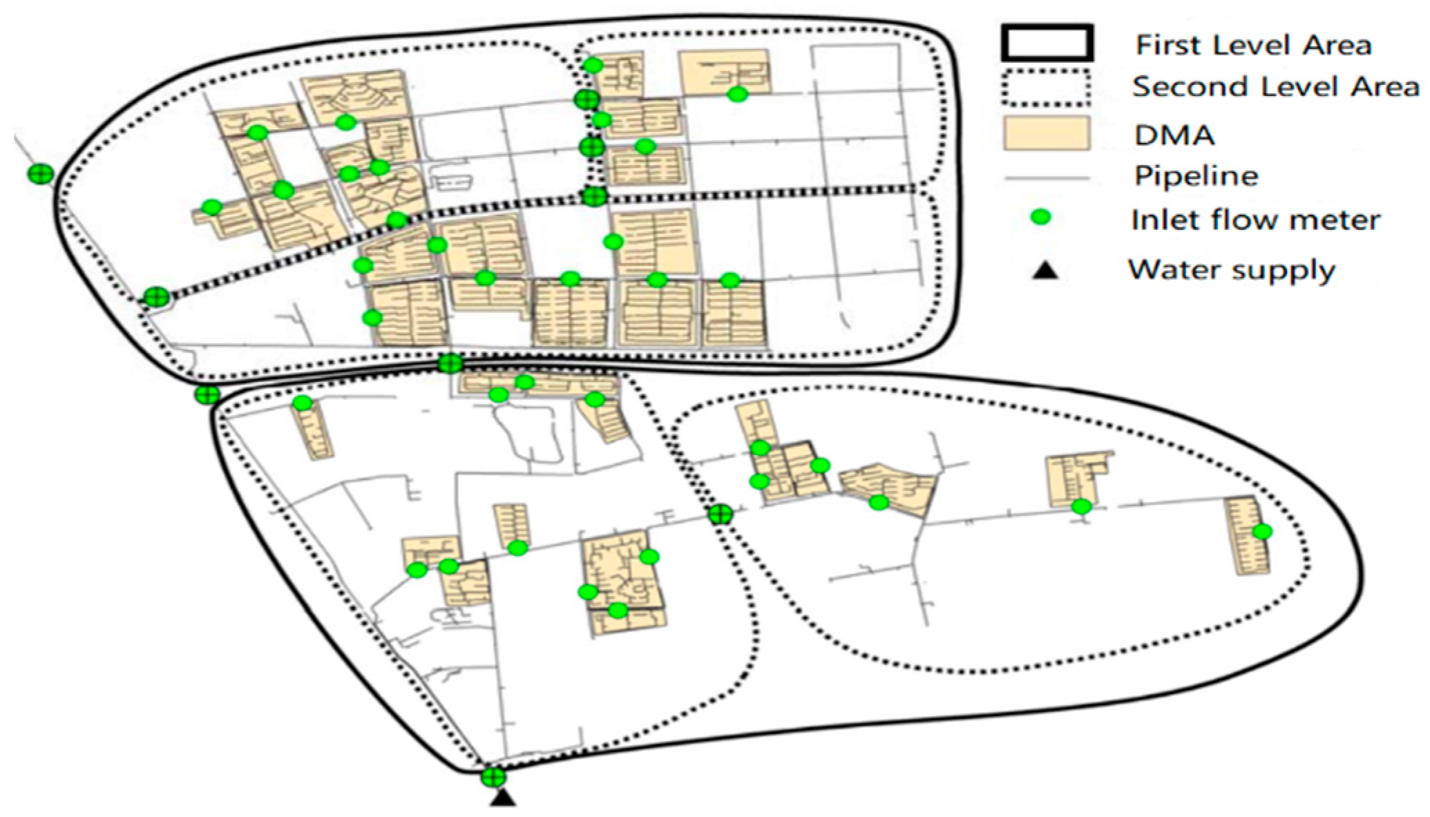
3.1. Flow Data Acquisition

The method proposed in this paper is applicable to burst detection and other abnormal flow events in DMAs [7]. In general, flow meters are installed at the DMA inlet and outlet. Flow meters typically sample data at fixed time intervals (e.g., 1 min, 5 min, 15 min), then send data to water supply companies at a fixed frequency (e.g., every hour, or a longer time interval) [8].

For example, the actual application was tested to verify the methodology using flow data of a DMA in a city in China. The water consumption was caused by almost all residents. There is a single flow sensor installed at the entrance of DMA. The flow meter collects the data at a fixed frequency of 15 min, then sends it to the water supply companies at a fixed frequency (every 2 h). Some statistical data about this DMA is described in

Table 2. Some statistical data about this DMA.

Month	Flow (m3/h)			Total Water Consumption (m3)	Daily Average Water Consumption (m3)
	Maximum	Minimum	Average
January 2018	21	4	10	8179	261
February 2018	19	4	10	7005
March 2018	19	6	10	8002
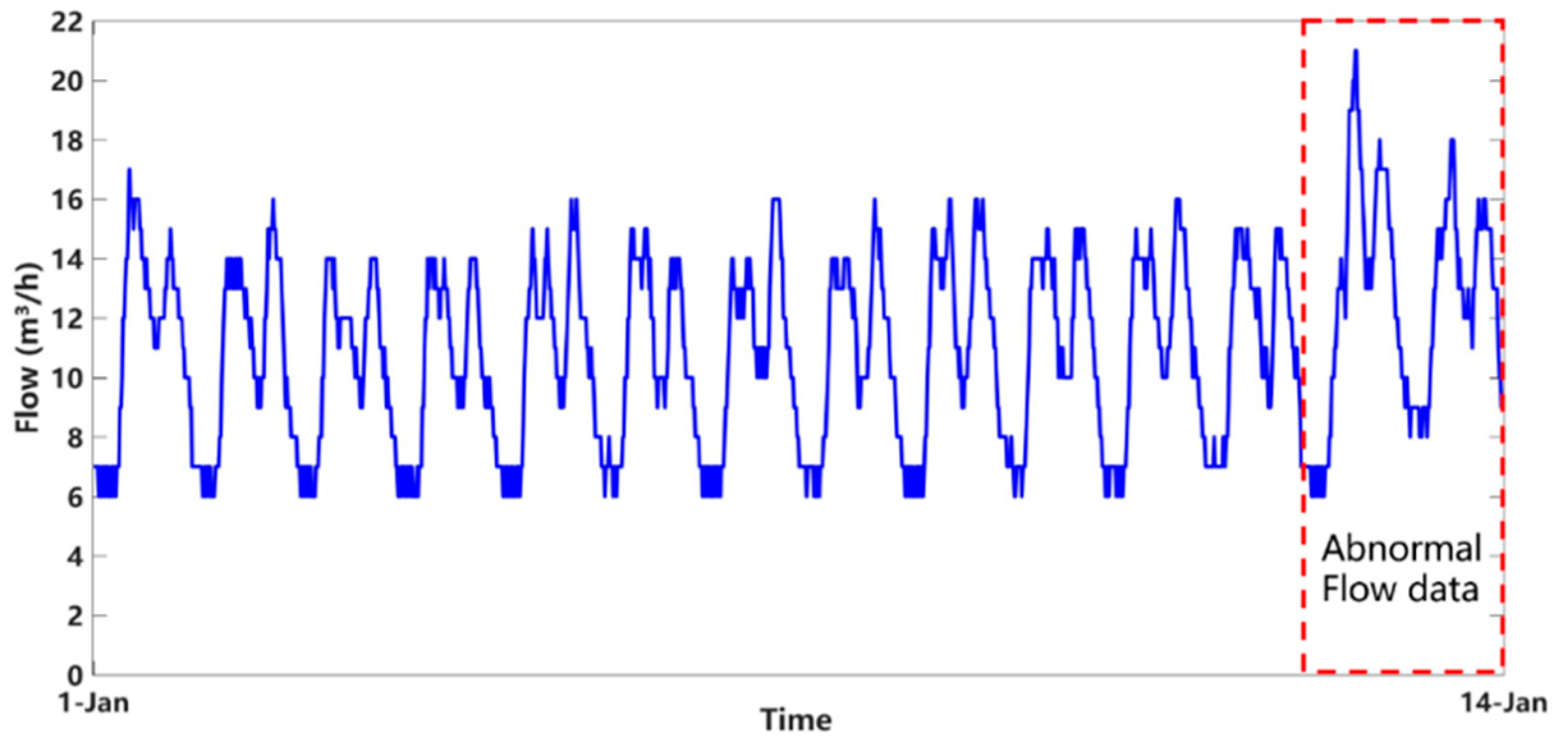
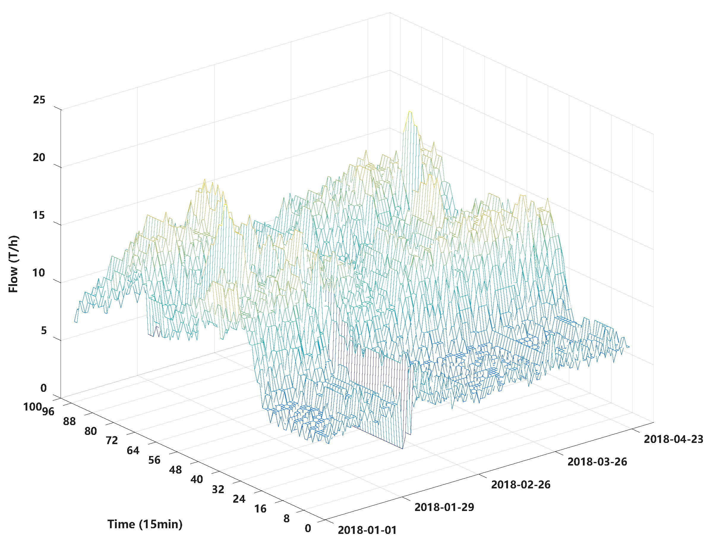
April 2018	21	5	11	8089

. Flow data from 1 January to 22 April 2018 (sixteen weeks) were used in this study for method evaluation, as shown in Figure 6.

As shown in Figure 6, the flow data change with time according to a certain period, but there are some differences in different periods. Flow data is a kind of pseudo-period data stream.

Water demand is greatly affected by consumer activities. This paper segments flow data into time intervals (24 h). Since the sampling interval was 15 min, there were a total of 96 sampling points in one day.

3.2. Results and Discussion About Patterns of Daily Water Demand

Sixteen weeks of flow data were studied using DTW. The ranking of abnormal probability of each day is from small to large, as shown in Figure 7.

According to abnormal probability, periods with large abnormal probability can be detected. which are defined as abnormal patterns of daily water demand. The corresponding date of abnormal patterns is shown in

Table 3. The corresponding date of abnormal patterns.

Date	Week	Date	Week
28 January	Sun.	19 February	Mon. (Festival)
29 January	Mon.	20 February	Tues. (Festival)
30 January	Tues.	21 February	Wed. (Festival)
31 January	Wed.	26 February	Mon. (Festival)
1 February	Thur.	2 March	Mon. (Festival)
2 February	Fri.	9 April	Mon.

.

Figure 7 and Table 3 indicate that patterns from Monday to Friday are very similar, but there are differences between weekdays and weekends. Obviously, patterns of festivals such as 19 February, 20 February, 21 February, 26 February, and 2 March (The Spring Festival in China) are different from non-festivals. For some seasons, such as when there are changes in pipe-network operating conditions, the patterns of water demand differ greatly to other patterns. As shown in Table 3, these patterns are defined as abnormal data from 29 January to 2 February and 9 April. These abnormal data must be removed to get a pure historical dataset. It is crucial to establish the corresponding burst identification model for different patterns of water demand. The original historical data on weekdays (Monday to Friday) and the normal historical data are shown in Figure 8.

Figure 8a,b depicts patterns of water demand as being more concentrated and regular after removing the abnormal patterns, indicating that the study of patterns of water demand is highly effective when based on DTW.

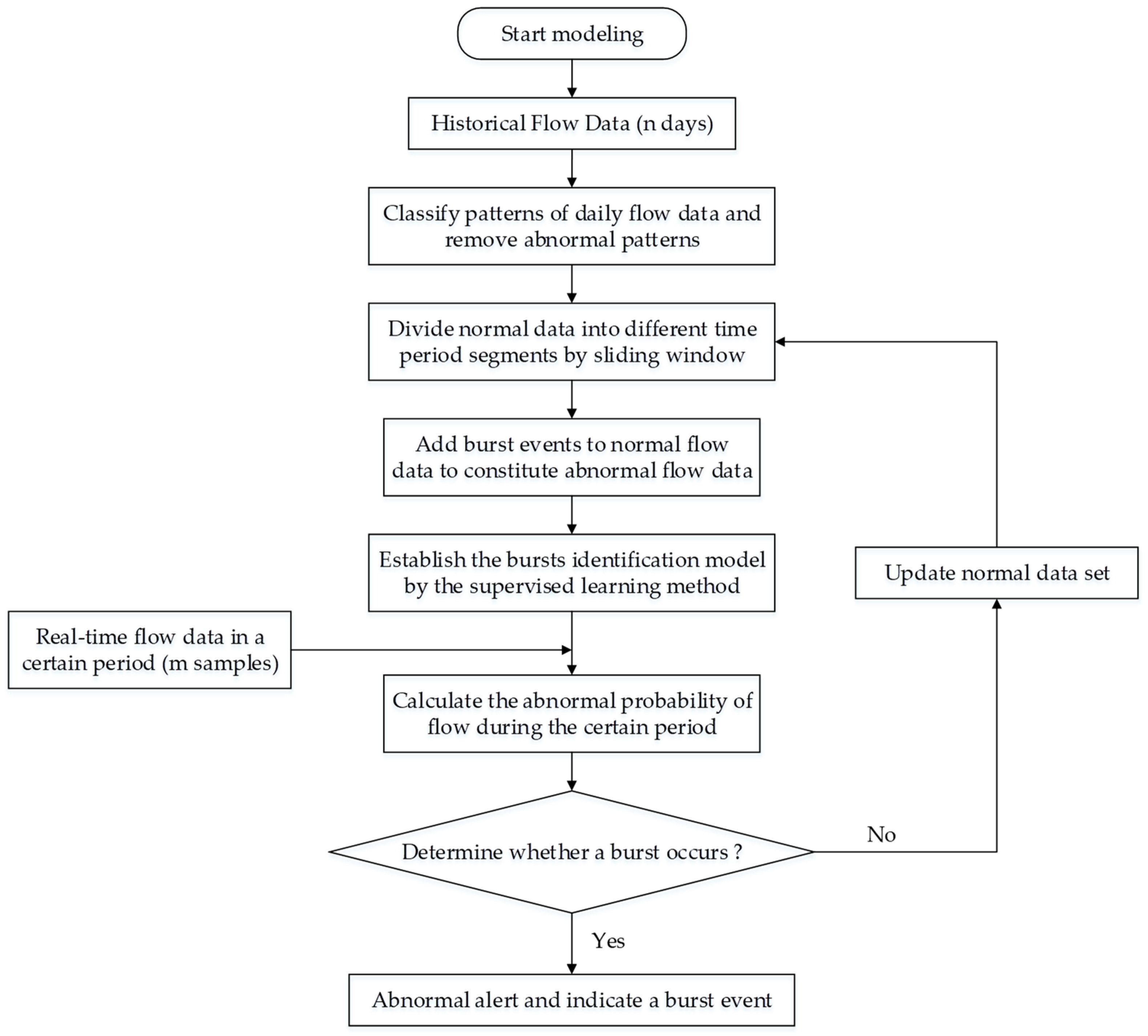
3.3. Results and Discussion About Burst Identification Method

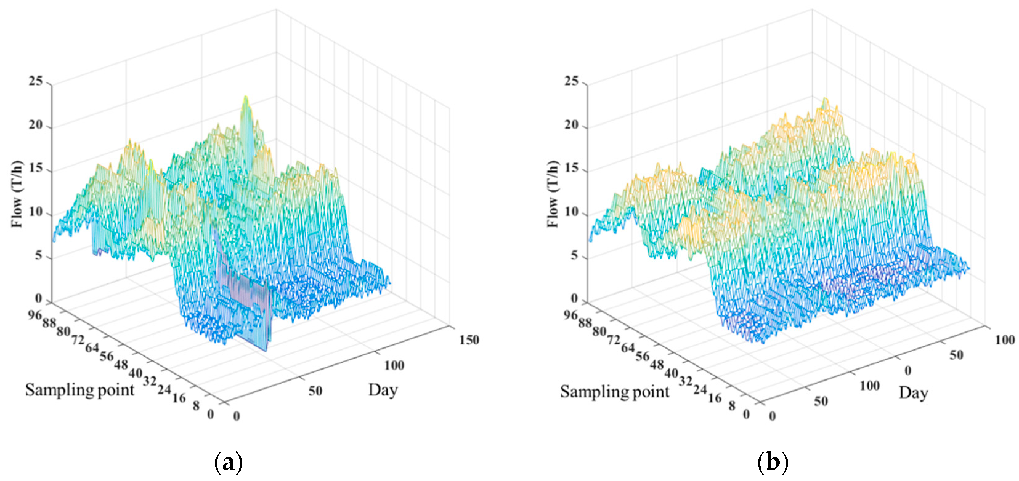
Flow data from 19 February to 8 June were acquired from a supervisory control and data acquisition (SCADA) system. Firstly, it needed to remove abnormal patterns in a historical dataset, and then to divide normal data into patterns on weekdays and weekends. The method was validated by simulating burst events through opening fire hydrants in the DMA [8]. Experimental information can be seen in

Table 4. Details about two simulated bursts in the DMA.

Leakage Event	Hydrant Opened Time	Hydrant Closed Time	Leakage Rate/(m3/h)	Percent Average Inflow (%)
E1	6 June 2018—9:30	7 June 2018—10:30	About 1.0	About 10
E2	7 June 2018—14:00	8 June 2018—15:00	About 2.0	About 20

.

Burst events where their size was 1 m³/h were attached to the normal dataset from 19 February to 8 June 2018 to obtain abnormal data with burst events. In order to have real-time burst detection, combined with the sampling frequency T (15 min) of the DMA sensors and the interval (every 2 h), the sliding time window can be set to eight sampling points (120 min ÷ 15 min). One day can be divided into 12 time periods, and the time window slides once every 2 h. This paper selected 60 days of historical dataset as the training dataset, with the next 10 days as the test dataset. The supervised learning method was used to train the model, and the corresponding burst identification method was modeled for twelve time periods (0:15–2:00, 2:15–4:00, 4:15–6:00, 6:15–8:00, 8:15:10:00, 10:15–12:00, 12:15–14:00, 14:15–16:00, 16:15–18:00, 18:15–20:00, 20:15–22:00, and 22:15–24:00).

Table 5. Parameters of the training model.

Parameters	Settings
Feature attribute variables	Flow data during 2 h
Amount of feature attributes	8
Number of trees	10
Amount of selection attribute randomly	6
Categories	Non-burst: 1; Burst: −1
Training dataset	Normal data: 60 days, Abnormal data: 60 days

shows the parameters of the training model.

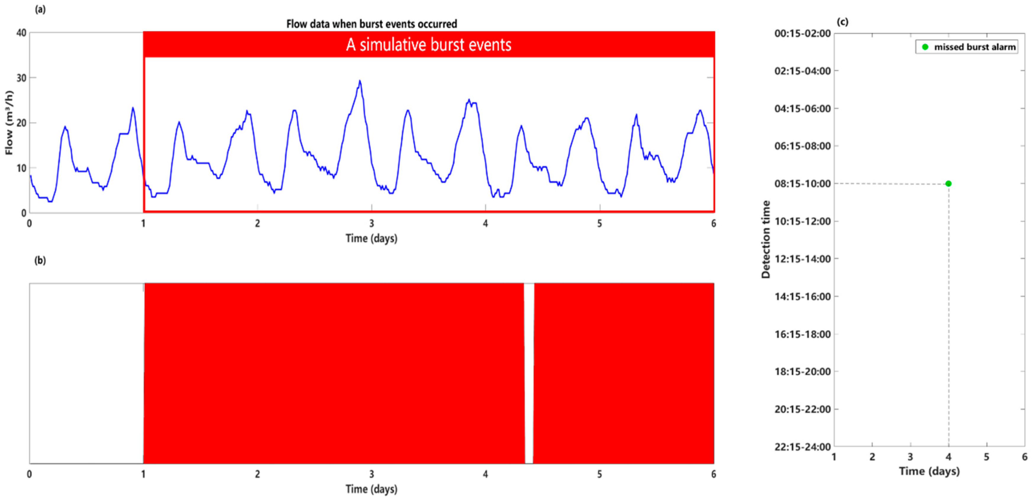
For instance, Figure 9 depicts the results obtained by burst identification, with patterns of the water demand system when burst events occurred. The observed flow data when simulative burst events occurred is depicted in Figure 9a, and the test result is depicted in Figure 9b. The red parts in Figure 9a indicate burst events. In Figure 9b, the red part indicates that bursts have been detected, and the blank part indicates no burst. Furthermore, the time of the missed burst detection is depicted in Figure 9c.

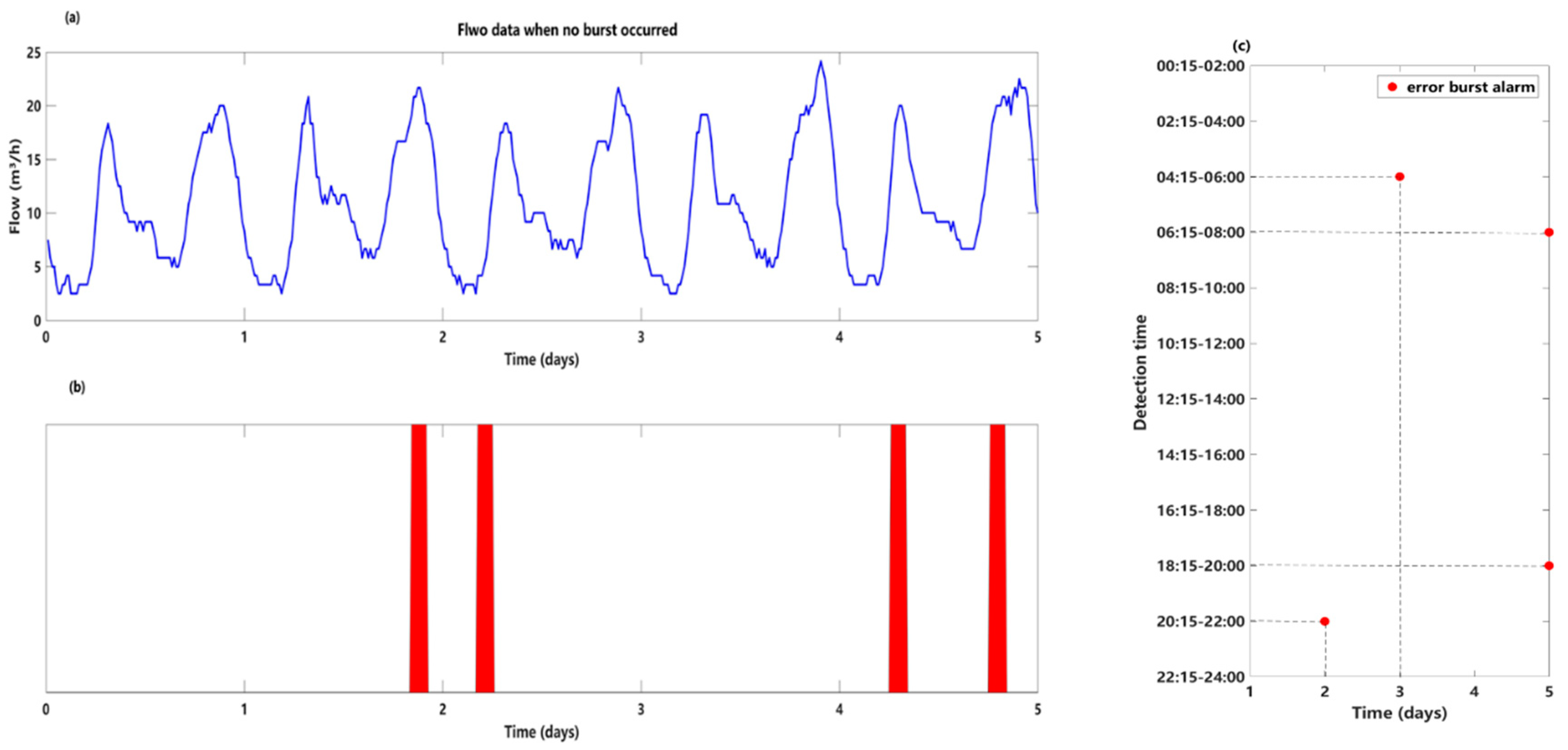
Conversely, Figure 10 shows the results obtained by a burst identification, with patterns of the water demand system when no burst event occurred. The observed flow data when no burst event occurred is depicted in Figure 10a, and the test result is depicted in Figure 10b. In Figure 10b, the red part indicates that bursts have been detected, and the blank part indicates no burst. The time of the false-burst alarm is depicted in Figure 10c.

TPR and FPR were calculated for burst identification with patterns of the water demand system. The system has a high TPR (98.3%) with a low FPR (6.7%).

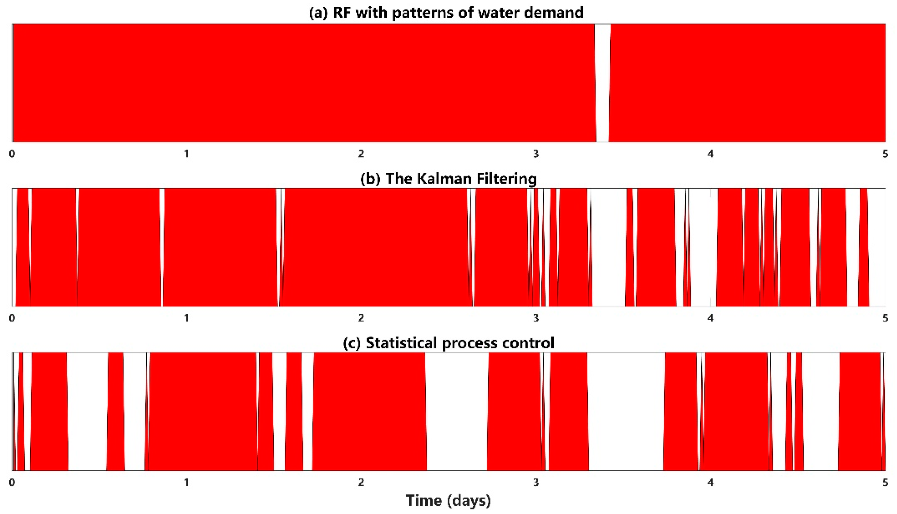
In previous research, most burst detection methods (prediction-classification, or statistical methods based on normal flow data) were tested and validated on DMAs. In this paper, the proposed method was compared with other methods, such as the Kalman Filtering (KF) method [27,28], and statistical process control (SPC) [29,30]. As a Detectability Comparison of random forest (RF) with patterns of water demand, the KF and SPC methods are depicted in Figure 11 and Figure 12. In these two figures, the red part indicates that bursts have been detected and the blank part indicates no burst. 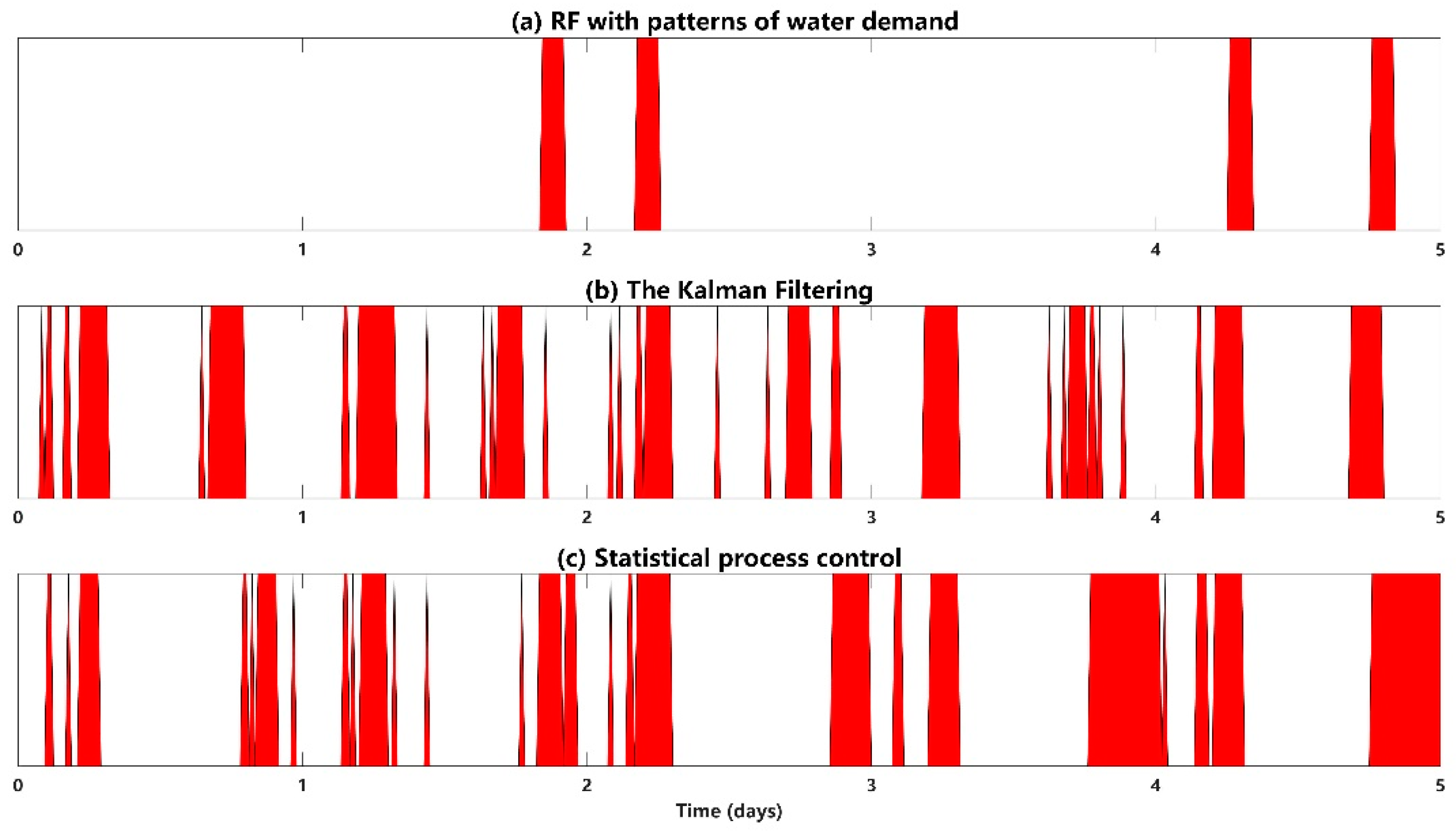Figure 11 shows the results of different methods when burst events occurred. On the contrary, Figure 12 shows the results of different methods when no burst event occurred. By observing Figure 11 and Figure 12, it’s obvious to draw a conclusion that the method proposed in this paper has a higher TPR and a lower FPR.

As shown in

Table 6. Detectability Comparison of RF with patterns of water demand, the Kalman Filtering (KF) and statistical process control (SPC) methods.

Methods	TPR (%)	FPR (%)
RF with patterns of water demand	98.3	6.7
The Kalman Filtering	77.5	26.9
Statistical process control	64.4	31.7

, compared with the KF and SPC methods, the proposed method performs better regardless of TPR or FPR. The SPC method is very ineffective for small bursts and large fluctuations in water demand. The main reason for this is that the SPC method is point anomaly detection based on statistical methods, and defines a normal range (mainly using the mean and the standard deviation). If the normal range is set to be small, false alarms are easily caused when the fluctuation of water demand is large. If the normal range is large, small burst events are easily ignored. Moreover, the Kalman filter is used to model normal water demand, and the residual between the predictive flow and the actual flow can indicate the size of bursts. Essentially, it is still point-anomaly detection, so when the water usage changes greatly, it can also easily cause false alarms. The burst detection method based on patterns of water demand and the Random Forest classification algorithm proposed in this paper has a lower false-alarm rate while being more sensitive to burst events. In actual situations, burst events in DMA rarely occur, so the false alarm rate should be as small as possible. Otherwise, a high false-alarm rate will bring unnecessary labor to the management of water supply companies.

In addition, using flow data between 2:00 and 4:00 at night, we compared the proposed method and the Minimum Night Flow (MNF) method, which is mostly widely used [31]. From

Table 7. Detectability Comparison of RF with diurnal demand pattern and Minimum Night Flow (MNF).

Methods	TPR (%)	FPR (%)
RF with patterns of water demand	100	0
MNF	100	10.5

, it is apparent that MNF is sensitive to small burst events (e.g., flow rate of 1 m³/h), but there are some false alarms. However, the proposed method in this paper is able to detect small bursts without false alarms.

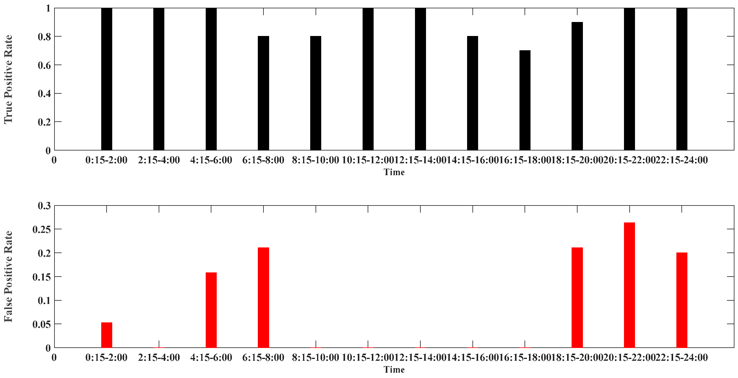
Since burst events may occur at any time, this paper studied the detection performance of the model at different time periods. The results are shown in Figure 13.

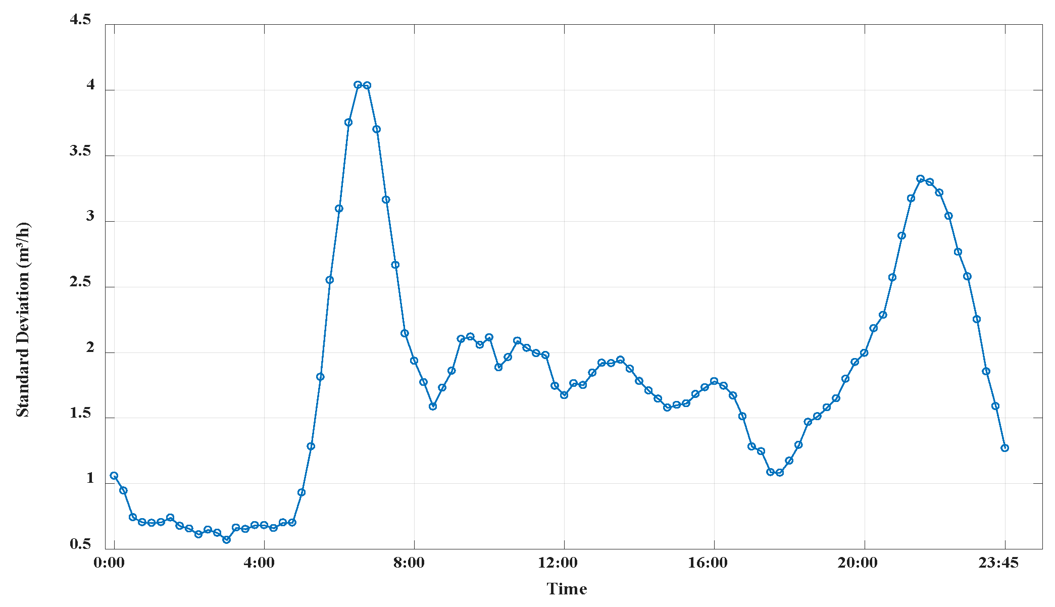
Figure 13 shows that false-positive rate is high between 4:15–8:00 and 18:15–24:00. This paper uses the standard deviation of flow at each time to reflect the magnitude of water fluctuations. Figure 14 shows the standard deviation of flow data at each time. It can be seen that the water usage varies relatively greatly during the two time periods of 5:45–8:00 and 19:45–23:00. This results in a high false-positive rate during periods when water usage fluctuations are large.

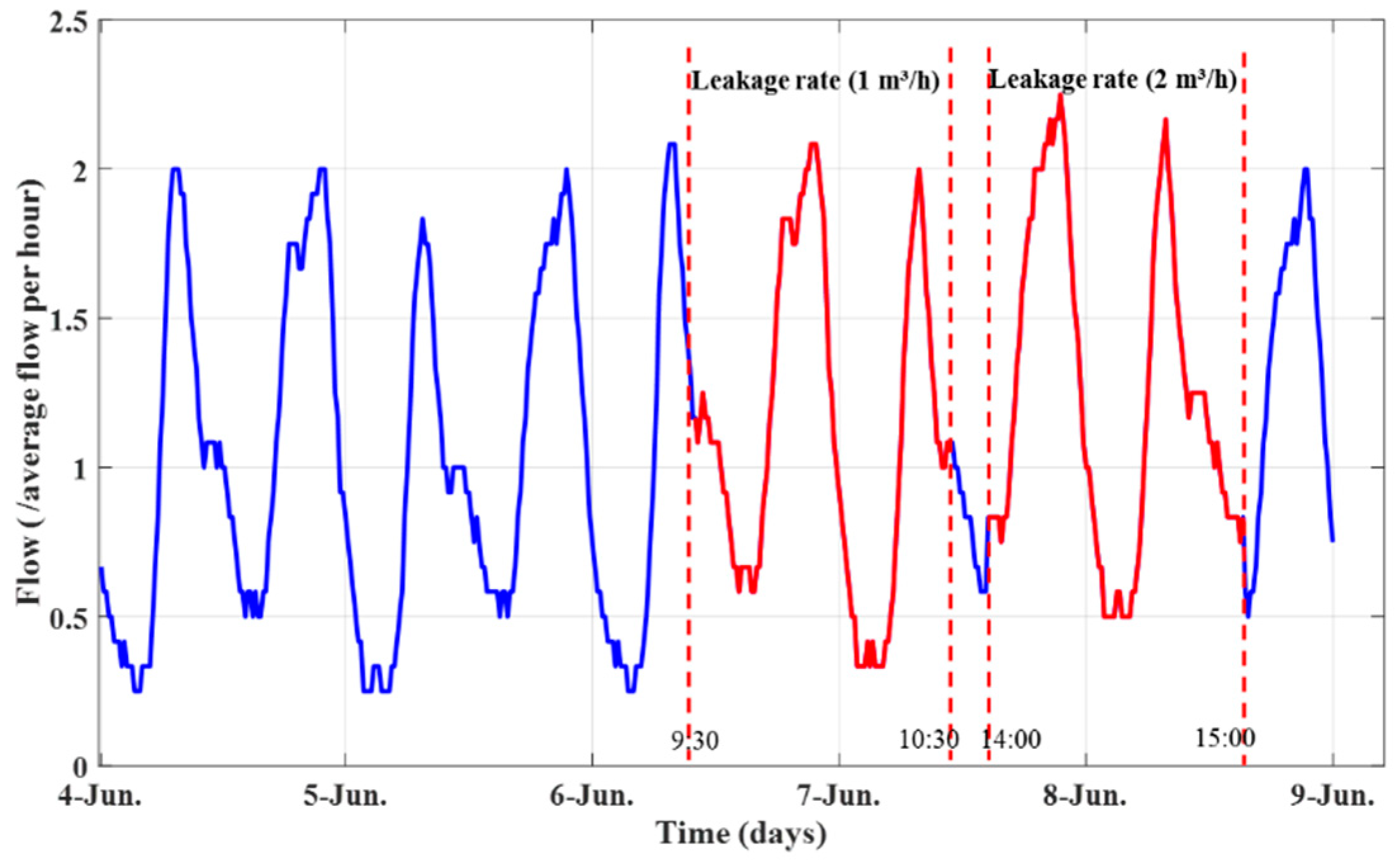
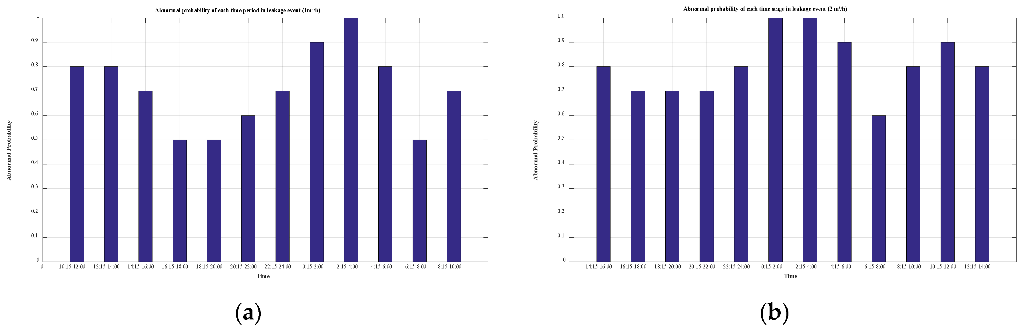
Finally, the simulated burst events from 6 June to 8 June 2018 were used to verify the proposed methodology. The red curve represents flow data under burst events, and the blue curve represents flow data under normal water demand (see Figure 15).

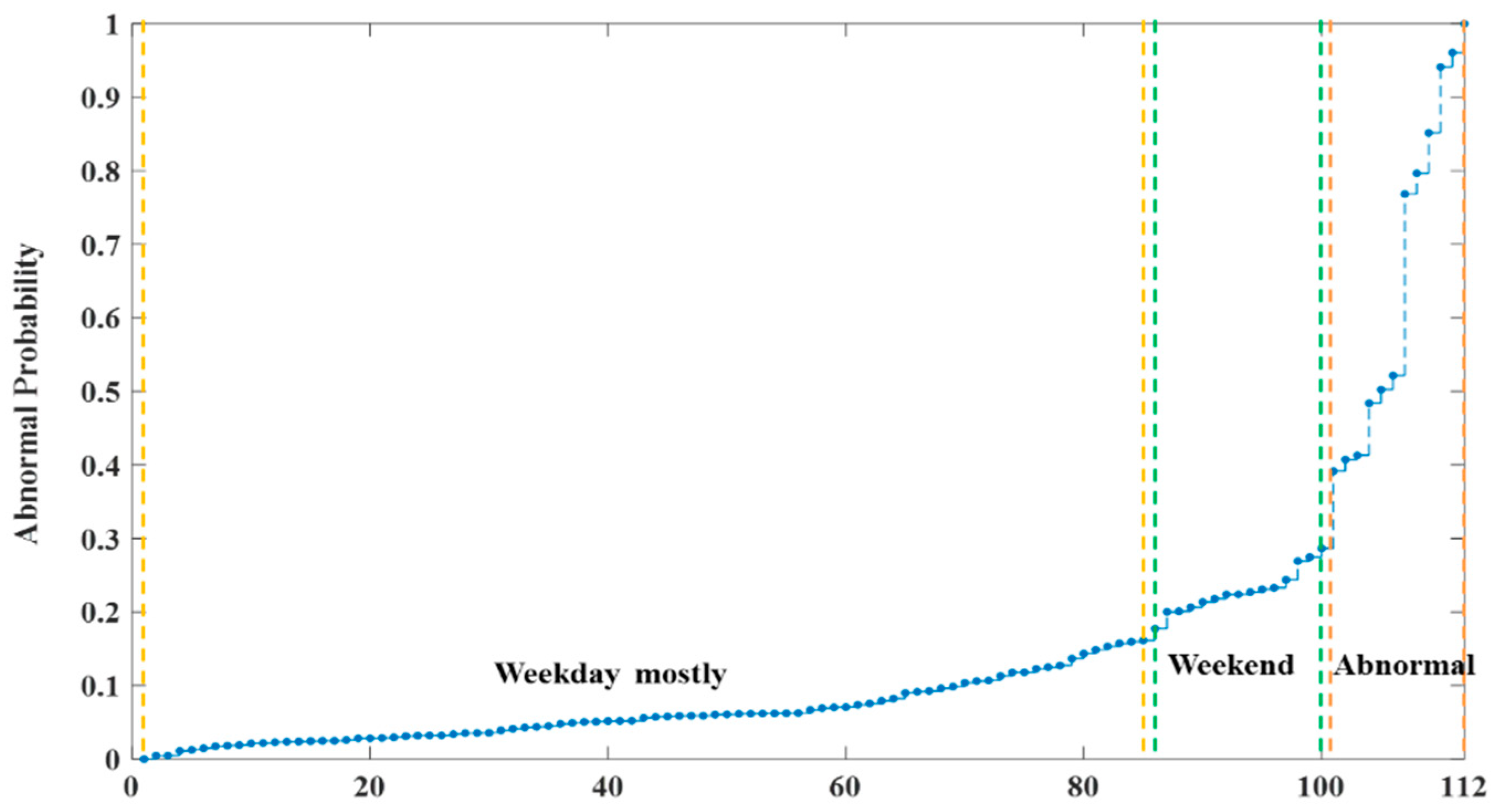
Figure 16a,b shows that when a burst occurs, the best detection time-period is between 2:15–4:00 at night. When the leakage rate is 10% of the average inflow per hour, the method could detect all burst events without a false alarm. Also, the larger the leakage rate, the easier it is to be detected. Burst detection in DMA can be modeled as a binary classification, so a threshold value is needed to distinguish whether bursts have occurred [32]. If the threshold of abnormal probability is set to 0.5, almost real-time rapid burst detection can be achieved.

4. Conclusions

The paper proposed a new burst detection methodology and showed the effect of the actual application in a DMA. According to the analysis results, it indicated that patterns of water demand and supervised learning methods can improve the effect of burst-event detection. Here are the following conclusions:

• This paper studied different patterns of water demand in a DMA. The method proposed can effectively remove abnormal historical data to obtain normal data, and distinguish different patterns of water demand using DTW. It fully considers the use of characteristics of DMA flow data.
• The proposed method had a better performance on real-time burst detection using supervised learning with patterns of water demand. It indicated that differentiating patterns of water demand could improve the accuracy of burst detection. Moreover, the performance of the burst detection is different at different time periods, with high accuracy at night (2:15–4:00) and low accuracy around breakfast time (5:45–8:00) or during early evenings (19:45–23:00). The advantage of burst detection based on the supervised learning method is that it can guarantee high accuracy and a low false-alarm rate, even if the burst is small.
• Although the methodology has a relatively low false-positive rate, some false alarms can still occur in the detection process, particularly if the consumption of consumers is unusual. Additional studies should be carried out in order to further decrease the false-alarm rate.

In summary, the proposed method can successfully detect bursts, with a low false-alarm rate and high accuracy. With the development of the SCADA system for urban water distribution networks, the proposed method shows great promise in its future application to DMAs.