Environmental Flow Assessment Considering Inter- and Intra-Annual Streamflow Variability under the Context of Non-Stationarity


1
State Key Laboratory of Eco-hydraulics in Northwest Arid Region of China, Xi’an University of Technology, Xi’an 710048, China
2
State Key Laboratory of Simulation and Regulation of Water Cycle in River Basin, China Institute of Water Resources and Hydropower Research, Beijing 100038, China
3
Environmental Change Institute, University of Oxford, Oxford OX1 3QY, UK
*
Author to whom correspondence should be addressed.
Water 2018, 10(12), 1737; https://doi.org/10.3390/w10121737
Submission received: 30 September 2018
/
Revised: 13 November 2018
/
Accepted: 23 November 2018
/
Published: 26 November 2018
(This article belongs to the Section Hydrology)
Abstract
:A key challenge to environmental flow assessment in many rivers is to evaluate how much of the discharge flow should be retained in the river in order to maintain the integrity and valued features of riverine ecosystems. With the increasing impact of climate change and human activities on riverine ecosystems, the natural flow regime paradigm in many rivers has become non-stationary conditions, which is a new challenge to the assessment of environmental flow. This study presents a useful framework to (1) detect change points in runoff time series using two statistical methods (Mann-Kendall test method and heuristic segmentation method), (2) adjust data of the changed period against the original flow series into a stationary condition using a procedure of reconstruction; and (3) incorporate inter- and intra-annual streamflow variability with adjusted streamflow to evaluate environmental flow. The Jialing to Han inter-basin water transfer project was selected as the case study. Results indicate that a change point of 1994 was identified, revealing that the stationarity of annual streamflow series is invalid. The variations of reconstructed streamflow series are roughly consistent with original streamflow series, especially in the maximum/minimum values and rise/fall rates, but the mean value of reconstructed streamflow series is increased. The reconstructed streamflow series would further serve to eliminate the non-stationary of original streamflow, and incorporating the inter- and intra-annual variability would upgrade the ecosystem fitness. Selecting different criteria for the conservation of riverine ecosystems can have significantly different consequences, and we should not focus on the protection of specific objectives that will inevitably affect other aspects. This study provides a useful framework for environmental flow assessment and can be applied to a wide range of instream flow management approaches to protect the riverine ecosystem.
1. Introduction
The integrity of riverine ecosystems and native biodiversity is the foundation of River Health [1,2]. However, human activities, such as water diversion, dam construction, and urbanization, have a variety of negative impacts on riverine ecosystems, and have changed the natural flow regime paradigm [3,4,5,6]. The change in the naturally variable regime of flow caused by human activities is regarded as one of the primary factors leading to the degradation of riverine ecosystems. Therefore, recent studies on environmental flow (EF) have shown that the natural flow regime paradigm, rather than just a specific low flow, is immediately required to sustain riverine ecosystems [7,8]. Assessment of EF based on the natural flow regime paradigm, therefore, becomes a reasonable procedure in designing measures for river protection and restoration. However, due to the impact of climate change and human activities, the natural flow regime paradigm in many rivers has presented non-stationary conditions, which is a new challenge to the assessment of EF [9,10,11].
Traditional methods of EF assessment are inappropriate for the management of riverine ecosystems when diverse human activities and climate change are taken into account [12,13]. The EF assessments, which are now widespread, promote the notion that traditional methods which are now common for site-specific assessment should be extended to include regional methodologies [14]. The trend of environmental water science is to integrate water resources management with flow-ecological modelling to balance the water demand of human society and freshwater biodiversity, and sustain riverine ecosystems and the ecosystem services they provide [4,15,16,17]. Because of the deterioration of ecosystems in many rivers around the world, river ecological protection has been received great attention. Though EF can be evaluated in a number of different procedures, almost all are dependent on two aspects: (1) sustain freshwater biodiversity and the integrity of riverine ecosystems with limited alterations from the natural flow baseline, and (2) preserve site-specific species and ecosystem service outcomes with designing flow regimes [18,19]. In practice, as the river authority struggles to preserve and restore riverine ecosystems, the former practice is needed to ensure that current ecological conditions of natural and semi-natural rivers do not deteriorate further. The later flow management is more applicable to the modified and regulated rivers where it is not feasible to revert to the natural conditions, and its primary objective is to maintain the important ecological processes and human well-being, i.e., through economic growth, population growth, and recreation. At present, a river basin is characterized by climate change and intensive management. Where hybrid and complex riverine ecosystems predominate, the best approach of EF requires extensive site-specific data and comprehensive modelling.
A key challenge for EF assessment in regulated rivers is to evaluate how much of the discharge flow should be retained in the river in order to maintain the integrity and valued features of riverine ecosystems [19]. Much research in recent years has established numerous formal methodologies for evaluating EF requirements. One of the best-known examples of EF assessment is the Ecological Limits of Hydrologic Alteration framework (ELOHA) [20], which was recommended by an assembly of agency scientists and NGOs. The ELOHA framework provided a scientifically-informed basis. It depends on the existing hydrologic and ecological databases from researchers and environmental water practitioners within a synthesis flow-ecological models for rivers to develop methodically viable and scientifically-testable hydrological characters for ecological responses revealed by flow alteration. These characters are achieved by four principal steps, and serve as the foundation for the societally-driven process of developing regional flow standards. The ELOHA framework and its derivatives are applied in many areas [21,22,23]. However, much research has recognized that the strength of the relationships between flow alteration and ecological responses is likely to be subject to numerous interpretations in many cases, which depend on the researcher’s expertise [24,25]. Scientific knowledge and information are not strong enough to establish an appropriate baseline in many areas; therefore, this acknowledged constraint has limited the availability of this framework.
Temporal variability is an important feature of natural streamflow. Generally speaking, the traditional method of EF assessment is to obtain different flow rates according to the different periods of the year, such as the flood season and dry season, which reflects the intra-annual streamflow variability in the EF. Furthermore, there is also inter-annual variation in the natural streamflow; this is also very important to biological survival and reproduction. Inter-annual streamflow variability is integrated into the ecological flow; it not only provides richer hydrological information for the ecological conservation, but can also alleviate conflicts between the water demand of ecosystems and human beings, especially in dry years [15,26]. However, few studies have considered the inter-annual streamflow variability in EF; therefore, this paper integrated inter- and intra-annual streamflow variability to divide the annual total runoff into different water years, and calculate the different EF for these water years.
The current EF science is based on long-term, historical patterns of flow stationary variability, which are no longer applicable to the current, non-stationary situation which is a consequence of intensified hydrological alteration [12,27]. Stationarity to streamflow is an opposite concept to non-stationarity. The stationarity of streamflow means that the statistical characteristics of historical streamflow have not been changed. Correspondingly, the statistical characteristics of non-stationary streamflow have been altered by climate change or human activates [28,29]. However, a few previous studies have taken into account the climatic and ecological non-stationary variability. In the last decade, it has become clear that the flow regime is changing due to human activities and global climate change on regional scales, where rapid global warming and global transformation of the land surface are causing means and variances of precipitation and streamflow to undergo significant changes [14,19,30,31,32,33]. These non-stationary conditions produce challenges for EF science in that hydrologic baselines are shifting, leading to historical hydrologic time series which are extremely questionable for use as stable conditions for EF practices [34,35,36]. These practices limit the use of historical conditions as a standard for restoration ecological benefits. Therefore, the most important task for EF assessment under non-stationary flow conditions is to adjust the non-stationary flow to return to stationary conditions. Furthermore, it is not possible to fully restore the time series of hydrological variability to the original conditions, and in practice, the key variables (e.g., seasonal, trend and maximum/minimum) [37] which are most closely related to the ecosystem should attempt to revert to the original conditions as much as possible.
At present, most research focuses on the study of ecological response under the context of non-stationarity, which is helpful for understanding the relationship between hydrological alteration and ecological response [5,9,25,38,39]. However, few studies have applied the ecological response to the procedure of EF assessment and the lack of a scientifically-feasible framework for the calculation of EF under the hydrological alteration. Hence, this paper attempts to deal with the non-stationarity of hydrological series from the perspective of Time Series Decomposition and Reconstruction, in order to ensure the consistency of key hydrological variables in the ecosystem.
The goal of this paper is to present a reasonable approach that incorporates inter- and intra-annual streamflow variability with the adjusted streamflow to investigate and synthesize obtainable scientific information into logic-based and socially-acceptable objectives for comprehensive EF management. This study was conducted to (1) detect change points in the annual streamflow series; (2) adjust the monthly flow for the changed period against the original flow series into a stationary condition; and (3) use the adjusted monthly streamflow and incorporate the inter- and intra-annual streamflow variability to evaluate EF. These issues were examined via a detailed case study of the Jialing to Han inter-basin water transfer project in China.
2. Study Area and Data
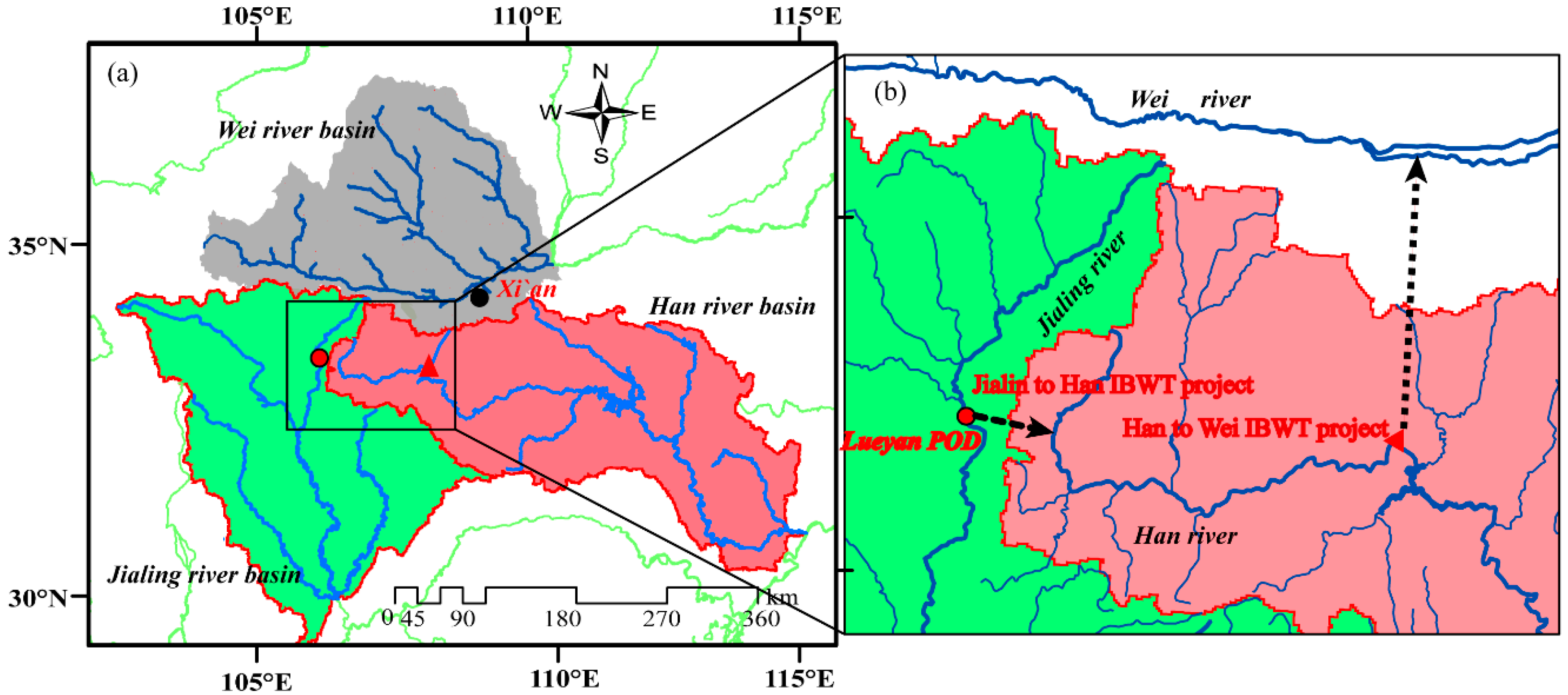
The Wei River is the foundation of human activities and multiple riverine ecosystems in the Guanzhong Plain of China, which sustains the drinking, industrial, and irrigation water of a total population of 22 million people in 76 major cities. Recent studies have shown that the Wei River runoff shows a decreasing trend, leading to serious water shortages and riverine ecosystem degradation problems because of the influence of climate change and human activities [40,41,42]. Therefore, the Han to Wei inter-basin water transfer (IBWT) project was conceived to solve this problem, which is the most significant water transfer project in Shaanxi province, China. The project is constructed across the boundaries of the Han River basin (donor basin) and the Wei River basin (recipient basin) in China.
The Han to Wei IBWT project is located in the upper reach of the Han River basin, and its main purpose is to alleviate water scarcity in the Wei River basin. The project is planned to divert water for 22 water use sectors, including industrial parks and urban cities, and to divert an annual average of 1000 million m3 (MCM) of water to the Wei River basin in 2025, and 1500 MCM water in 2030. It should be noted that the Han River has been selected as one of the water sources for the south-to-north water transfer project (the world’s largest IBWT project), and the runoff is diverted primarily to satisfy the water resource demand of the south-to-north water transfer project. For this reason, the transferable water amount of the Han to Wei IBWT project is subjected to 2200 MCM in wet year and 7 MCM in dry year by the Changjiang Water Resources Commission (CWRC). Due to constraints, the Han to Wei IBWT project cannot satisfy the water demand of the central plain, and the efficiency of the project also cannot be fully achieved. Therefore, the Shaanxi provincial government recommended a new water transfer project of the Jialing to Han River IBWT Project to make up for the shortfall.
The Jialing to Han River IBWT Project is being planned; it will see construction across the boundaries of the Jialing River basin (donor basin) and the Han River basin (recipient basin), and divert an annual average of 500 MCM of water to the Han River basin in 2030 (Figure 1). In this project, the role of the Han River basin will be conversed from donor basin to recipient basin, and the Han River will have sufficient water resources to meet the water demands of the human and riverine ecosystem. The Jialing to Han River IBWT Project is located in the upper reach of the Jialing River basin, and the point of diversion (POD) of the project is located on the Lueyang County, Shaanxi Province. According to the design information (obtained from the Water Bureau of Shaanxi Province.), the project will divert the flow rate of 40 m3/s from the POD, and discharge the EF of 21.6 m3/s (20 percent of annual average runoff), to protect the multiple riverine ecosystem of the down reach in the POD. However, with climate change and human activities, the streamflow of the Jialing River has changed; as such, the riverine ecosystem cannot be sufficiently protected by the planned EF.
In this study, monthly streamflow data were used to restore data homogeneity. Then, the EF was calculated using the adjusted data in the POD. The calculated and planned EF were used as the constraints of a diverted process and for comparison with each other.
3. Methodology
The goal of this section is to introduce an approach of EF assessment for ecosystem protection that is adapted to the changed streamflow regime of the Jialing river streams in nonstationary conditions. Key procedures for EF assessment in Jialing river streams include: (1) the Mann-Kendall (MK) test method and heuristic segmentation method, to identify change point in the streamflow time series; (2) the data of the changed period against the original flow series were adjusted by using the Seasonal-Trend Decomposition based on Loess smoothing (STL); (3) the adjusted flow series was divided into wet, normal, and dry years by using the standardized precipitation index (SPI); (4) the EF with different water years was evaluated using the percent of flow approach; (5) the planned and calculated EF were compared, and detected the most comprehensive policy for the conservation of riverine ecosystem.
3.1. Change Point Analysis Method
At present, there are many traditional statistical test methods for identifying the change point in the time series, like the sliding F test, sliding T test, and rank sum test. These methods are limited to a specific time series, and are highly dependent on the assumption that the time series is stationary and linear [43]. The limitation leads to a further reduction of its flexibility. For nonstationary and nonlinear time series, these conventional methods make it difficult to accurately identify the real change point in the time series. In this paper, we selected the MK test method [44,45] and the heuristic segmentation method to identify the possible change point. The following section is a brief description.
The MK test method is a nonparametric statistical test method which has been widely used throughout the world. H. Bmann and M.G. Kendall (1975) proposed the principle and developed the method, which can detect the trend and change point of time series. The MK test method does not require a preset length for the time series. However, it is difficult to use the method for time series with multiple variables or multiple scale mutations. The specific calculative processes can be referred to [46,47].
The hydrological time series is influenced by climate change and human activities, and it often presents a high degree of nonlinearity and non-stationarity. The traditional statistical test method is used to detect the change point of hydrological time series, which often produces a certain deviation. The heuristic segmentation method proposed by Pedro et al. (2001) [48] is mainly used to identify the change points of mean values for nonlinear and nonstationary time series. Due to the method adopting an iterative algorithm in Split, it significantly reduces the computational cost and has a great practicability. Compared with traditional method, the heuristic segmentation method can be used to segment a nonstationary time series into several stationary subseries, and it can overcome the shortcomings of conventional methods. Therefore, this study also used the heuristic segmentation method to identify the change point of annual streamflow series in the Jialing River.
3.2. The Decomposition Procedure
Decomposition is a statistical method that disects a time series into several components; each represents one of the feature-based subseries. A time series is usually decomposed into Trend, Seasonality, and Reminder, respectively [49]. The three components can be obtained using an additive mode, which is shown as follows:
where Yt is the time series at time t, Tt is the trend component at time t, St is the seasonal component at time t, and Rt is the reminder component at time t.
In this study, the decomposition of time series into trend, seasonality, and reminder components was performed in the R-software package using the STL. It is a popular algorithm in time series decomposition, which is based on the loess approach to decomposing the data of a certain moment into the trend component, seasonal component, and remainder component. The calculation process of the STL is divided into inner and outer loops, in which the inner loop mainly does the calculation of trend fitting and periodic component and the outer is mainly used to regulate robustness weight [50,51].
The procedure is accomplished in a circulation of detrending and then updating the seasonal component from the resulting subseries. At every iteration, the robustness weights are formed based on the estimated irregular component; the former is then used to down-weight outlying observations in subsequent calculations. The iterated cycle is therefore composed of two recursive procedures, the inner and outer loops. Each pass of the inner loop applies seasonal smoothing that updates the seasonal component, followed by trend smoothing that updates the trend component. An iteration of the outer loop consists of one iteration of the inner loop, with the resulting estimation of the trend; seasonal components are used to calculate irregular components. Any large values are identified as extreme values, and a weight is calculated. This concludes the outer loop. Further iterations of the inner loop use the weights to down-weigh the effect of extreme values which were identified in the previous iteration of the outer loop. Compared with other decomposition procedures, the significant performance of the STL is strong resilience to outliers in the data, resulting in a robust subseries. For a more detailed description of the STL decomposition procedure, the reader is referred to Cleveland et al. (1990) [49].
3.3. Standardized Precipitation Index (SPI)
The Standardized precipitation index (SPI) [52,53] is a method for analyzing the characteristics of drought (frequency, duration, spatial distribution pattern, and intensity) by using the long series of precipitation data. The SPI is employed to characterize the probability of precipitation in a certain period of time, and it is appropriate for drought monitoring and evaluation relative to the local climatic conditions on a monthly time scale [54,55]. The Gamma distribution is used in SPI to identify the change of precipitation, and the cumulative probability distribution is transformed into the standard normal distribution. Normalized precipitation cumulative probability distribution is used to classify the drought grade. Due to its simplicity and low data requirements, it has been widely used [56,57,58].
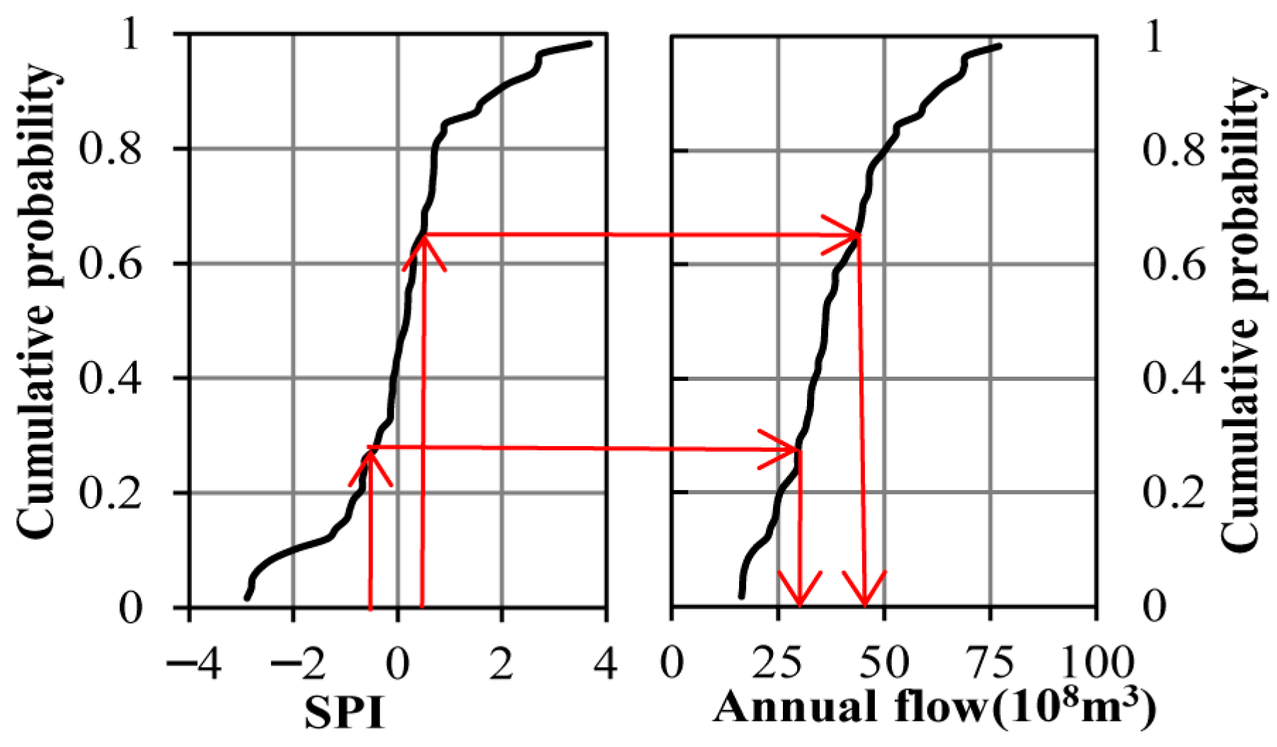
In this study, considering the inter-annual variability of streamflow, the annual streamflow monitoring data of the Jialing River is dissected into three typical series (wet, normal and dry) by using the SPI [15]. The calculation formula is as follows:
where r is the annual runoff, FR is the cumulative probability distribution of the annual streamflow, and Φ−1 is the inverse standard normal distribution.
According to the definition of the SPI, the values of SPI greater than 0.5 are classified into the wet years, the values of SPI less than −0.5 are classified into the dry years, and the values of SPI ranging between −0.5 and 0.5 are classified into the normal years. The detail of the calculation process and the criteria are described in Svoboda et al. (2002) [59].
3.4. Percent of Flow Approach
Many traditional methods of environmental flow assessment can only be applied to specific regions because of need for massive amounts of site-specific data, expensive modeling, or both. Furthermore, they often do not preserve the full range of variability in the riverine ecosystem. The percent-of-flow (POF) strategy is a holistic flow management strategy, and is designed to preserve multiple riverine ecosystems and protect intra-annual flow variability [60,61]. The site-specific POF procedure usually requires unimpaired or historic flow information, and its lack of universality protects the natural flow regime. Although there is limited guidance for what small, or minimum flow should be allocated by the POF procedure to protect riverine ecosystems, according to the law of tolerance, there are natural minimum and maximum thresholds of flow which handle the survival and development of riverine biology [62]. While allocating the EF below the minimum threshold, riverine ecosystems will cause an irreversible deterioration [63,64]. Therefore, in practice, a minimum EF process is needed to protect the river ecology. Based on a review of previous studies, this paper identified the EF using the monthly 90th percentile exceedance values of flow with different water years in the POD.
3.5. Range of Variability Approach (RVA)
The indicators of hydrological alteration (IHA) statistical method is recommended by Richter et al. (1997) [65,66]; it is used to characterize within-year variation in stream flows. Richter analyzed the rationality and adaptability of the IHA, and proposed a further method—the range of variability approach (RVA)—which is used to calculate the degree of alteration for each hydrologic parameter in IHA. The RVA method serves to compare the two periods of a hydrologic time series, and the RVA values are organized into five statistical groups to estimate the hydrological parameters between the pre-impact stream flow (natural flow) and the post-impact stream flow. The five groups simply denote a noticeable and significant alteration in stream flow characteristics, including magnitude, timing, frequency, duration, and rate of change of flow.
This statistical method defines the target ranges (between 25th percentile value and 75th percentile value) to partition the full range of pre-impact data into different categories: low category, middle category, and high category. The degree of stream flow alteration, Di, is calculated as:
where No and Ne are the expected and observed numbers of years whose RVA values fall into the target ranges during the post-impact flows, respectively.
Synthetic hydrological alteration, D0, is evaluated by the following:
3.6. Indicators of the Intra-Annual Variability of Streamflow
In this study, six statistical coefficients (nonuniformity coefficient (Cn), complete accommodation coefficient (Cc), concentration degree (Cd), concentration period (Cp), relative variation range (Cr), and absolute variation range (Ca)) were used to comprehensively estimate the characteristics of intra-annual streamflow variations.
The nonuniformity coefficient (Cn) and complete accommodation coefficient (Cc) are used to estimate the variation of intra-annual streamflow; they are formulated as follows:
where Q(t) is the monthly flow and
is the average of monthly flow.
The concentration degree (Cd) typically indicates the degree of concentration of the intra-annual distribution of flow, and the concentration period (Cp) reflects the concentration of flow in one year. They are formulated as follows:
where , , .
where Qx and Qy are the two resultant vectors of Q(t) that are decomposed in the x direction and y directions, respectively; Qxy is the module of the vector, and θ(t)=2πt/12 is the angle of the vector for month t.
The relative variation range (Cr) and the absolute variation range (Ca) were used to estimate the range of monthly flow distribution, where Cr is the ratio of maximum annual flow to minimum annual flow, and Ca is the absolute deviation between those two values. They are formulated as follows:
where Qmax and Qmin are the maximum and minimum monthly flows, respectively.
4. Results of Environmental Flow Assessment
4.1. Identifying Runoff Change Point in the POD
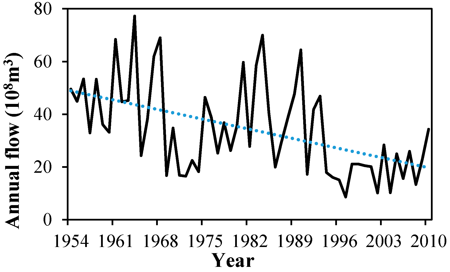
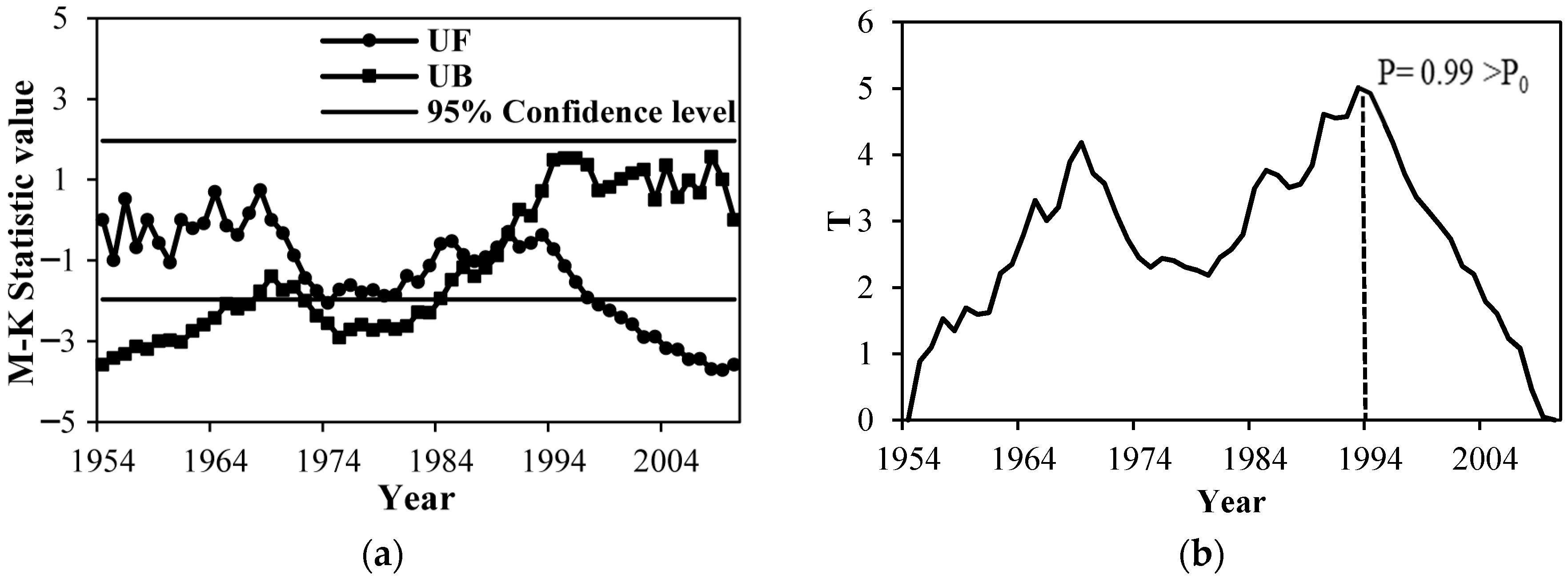
For the POD of Jialing River, annual streamflow data with 1954–2010 (Figure 2) at the Lueyang hydrological monitoring station were used to identify the change points using the Mann-Kendall test method and the heuristic segmentation method, respectively (Figure 3). As shown in Figure 2, there was an obvious decrease in streamflow, and the flow magnitude was smaller in general at the POD after 1990, which was significantly affected by climate change. Because the upstream of the POD is a remote mountainous area, no water conservancy project has been constructed, and the area almost unaffected by human activities. Figure 3a shows the statistical variation of the UF and UB of the Mann-Kendall test method which determines the change point in annual streamflow at the POD. The change point was in the time period from 1990 to 1994.
Figure 3b presents the statistical variation of the heuristic segmentation method which calculates the variance between the averages of the right- and left-side subseries of annual streamflow data. In this study, the threshold P0 was carefully chosen as 0.95, and l0 was selected as 25. As shown in Figure 3b, the identification results of change points in the annual streamflow data is 1994, because the probability of the largest T is greater than the threshold (P0). Based on the results of the previous two methods, the variations of the annual streamflow data at the POD are obvious, and the change point in the series is 1994. Therefore, according to the time of change point, the streamflow data from 1954 to 2010 can be divided into two periods: the pre-impact (natural) series (1954–1993), and the post-impact (changed) series (1994–2010), respectively. We used the homogeneity of the pre-impact series to restore the non-stationary post-impact series, and then integrated the pre-impact series and the adjusted series to calculate the EF in the POD in the following sections.
4.2. Reconstructing Streamflow Series
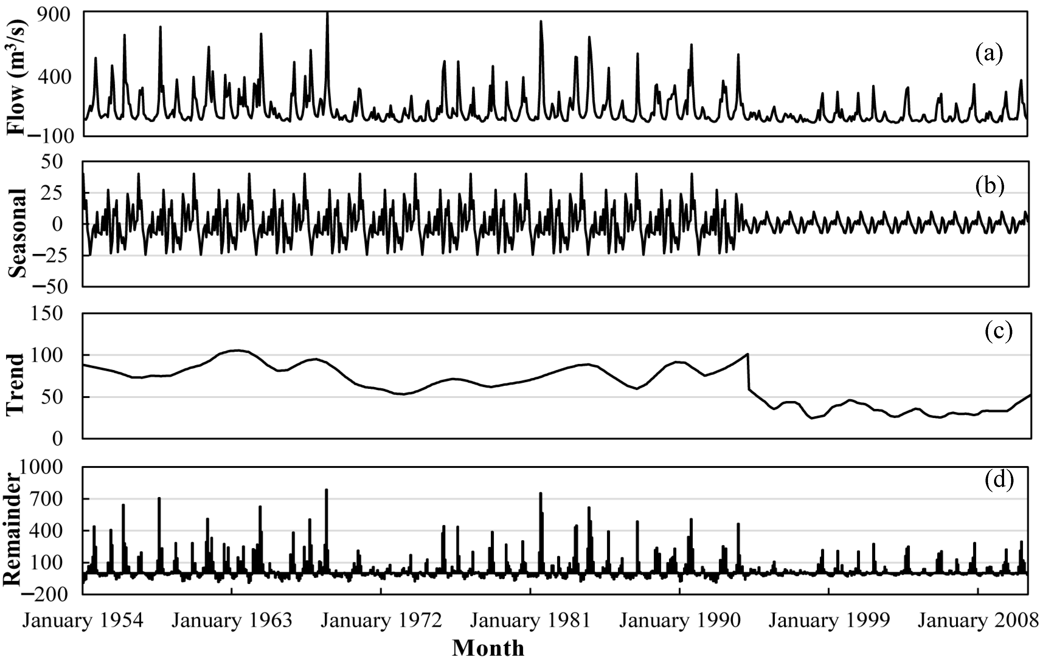
The STL decomposition method was adopted to decompose the component of monthly streamflow series in the pre-impact (natural) series (1954–1993), and the post-impact (changed) series (1994–2010), respectively. The decomposition of monthly streamflow series into seasonal, trend, and remainder components was implemented in R-software (http://www.r-project.org) by using the function—stl, and the results of the application of the STL decomposition procedure are presented in Figure 4. As can be seen from Figure 4a, monthly streamflow measured at the POD is greatly altered. Referring to Figure 4b,c, these impacts are also observable in the seasonal and trend components decomposed from the monthly streamflow series, and these statistical values of the post-impact series are smaller than the pre-impact series. The remainder component of the monthly streamflow series is depicted in Figure 4d, which is usually identified as the noise component of a time series, and is affected by most different factors. In the monthly streamflow series, the remainder component is significantly controlled by the condition of the land surface and the local climatic conditions.
In this study, series homogeneity between the pre-impact series and the post-impact series at the considered change point was achieved by processing data from the post-impact series in an additive procedure: (1) directly copy the seasonal and trend components of the pre-impact series onto the post-impact series, and (2) recombine (i.e., by addition) the streamflow components to adjust total streamflow conditions prior to pre-impact conditions. Figure 5a shows the result of the reconstructed monthly streamflow series in 1994–2010. It can be seen from Figure 5a that the variations of reconstructed streamflow series are roughly consistent with the original streamflow series, especially the maximum/minimum value and rise/fall rate, because the remainder component of the original streamflow series was preserved by the procedure of reconstruction.
For a better comparison, the original annual streamflow series (1954–2010) and the reconstructed total annual streamflow series are plotted in Figure 5b. The reconstructed total streamflow series does not show an obvious trend in all time periods. In addition, the identification of the change point in the reconstructed series based on previous test methods, and the no change point, was observed. Therefore, the reconstructed procedure has acceptable performance in processing data homogeneity, and can be applied in this paper to eliminate the inconsistencies of streamflow series.
4.3. Assessing the Environmental Flow
In this study, we proposed an approach which was adopted to calculate the EF in the POD. It takes into account the inter- and intra-annual streamflow variability. The inter-annual streamflow variability was considered as a long-term variation of streamflow, and the streamflow was classified into wet, normal, and dry years with a statistical method to identify the practical management units. In different management units, the environmental flow for the POD is based on a percentage of the streamflow baseline, calculated as the monthly 90th percentile exceedance flow. There are two basic steps to this proposed approach:
Step 1: classify annual streamflow into wet, normal, and dry years using the SPI. The reconstructed annual streamflow (1954–2010) at the POD can be best fitted with a Gamma distribution; its alpha and beta parameters (set to 7.19 and 5.40, respectively) were determined by the method of maximum likelihood. Therefore, the threshold annual streamflow used to classify the wet and dry years are 4372 and 2973 MCM, respectively, and the results of the classification are shown in Figure 6. It can be seen from this figure that the resulting numbers of the dry, normal, and wet years are 16, 21, and 20, respectively.
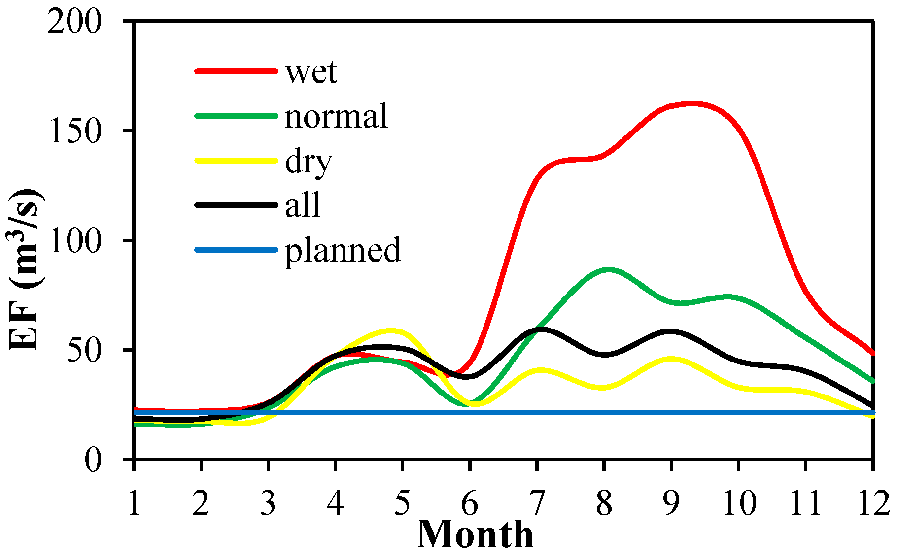
Step 2: Calculate the EF in each group. The different water years have been identified in step 1, and the approach for applying each group in the environmental flow assessment is as follows: (1) the monthly streamflow data in each year of each group (e.g., wet years) can be plotted on common axes (Figure 7); (2) the array of streamflow values in each month is selected and the data is ranked to choose the value exceeded by 90% of the values for calculating the monthly 90th percentile exceedance value. The monthly 90th percentile exceedance values are identified as the EF in each group and the calculated EF shown in Table 1 and Figure 8. Here, the calculated and planned EF of all years also is shown in Figure 8.
It can be seen from Figure 8 that the conflict of water resources between river protection and human demand is more serious in the dry season. Decision makers are more concerned about the utilization of water resources in the dry season, and the allocation of water resources depends more on the preferences of decision makers; it is difficult to ensure the effectiveness and equity between river protection and human demand in decision-making. As shown in Figure 8, the calculated EF is approximately consistent with the planned EF in the dry season, which can easily be accepted by decision makers. However, the calculated EF improved significantly in the wet season, and it is the key factor for the protection of multiple riverine ecosystems.
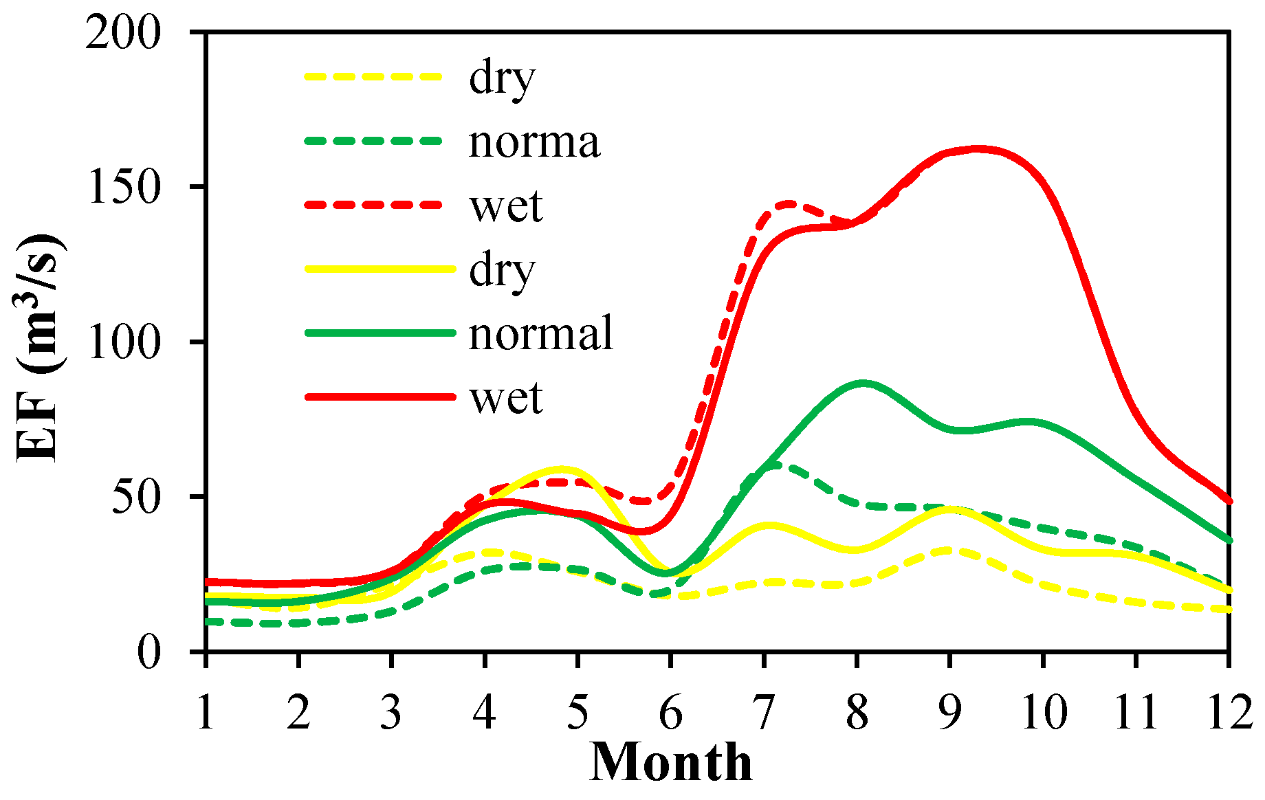
In order to further access the benefits of calculated EF, the two steps were also used to calculate the EF of the original (without reconstruction) streamflow (1954–2010) at the POD. The first step is to classify original annual streamflow into wet, normal, and dry years, and the second is to calculate the EF of different water years. The results of the EF of the original streamflow at the POD are shown in Figure 9 (the dotted lines are the EF of the original streamflow, and the solid lines are the EF of the reconstructed streamflow). It is apparent from this figure that the EF of the reconstructed streamflow is greater than the EF of the original streamflow in normal and dry years; however, the EF of the reconstructed and original streamflow have shown a similar tendency in the wet years. The reason of the different results is that the procedure of reconstruction pays more attention to the mean and minimum streamflow value than the maximum streamflow value; therefore, this differential response in the EF is that there is more or less consistency in the wet years, but that it improved in the normal and dry years.
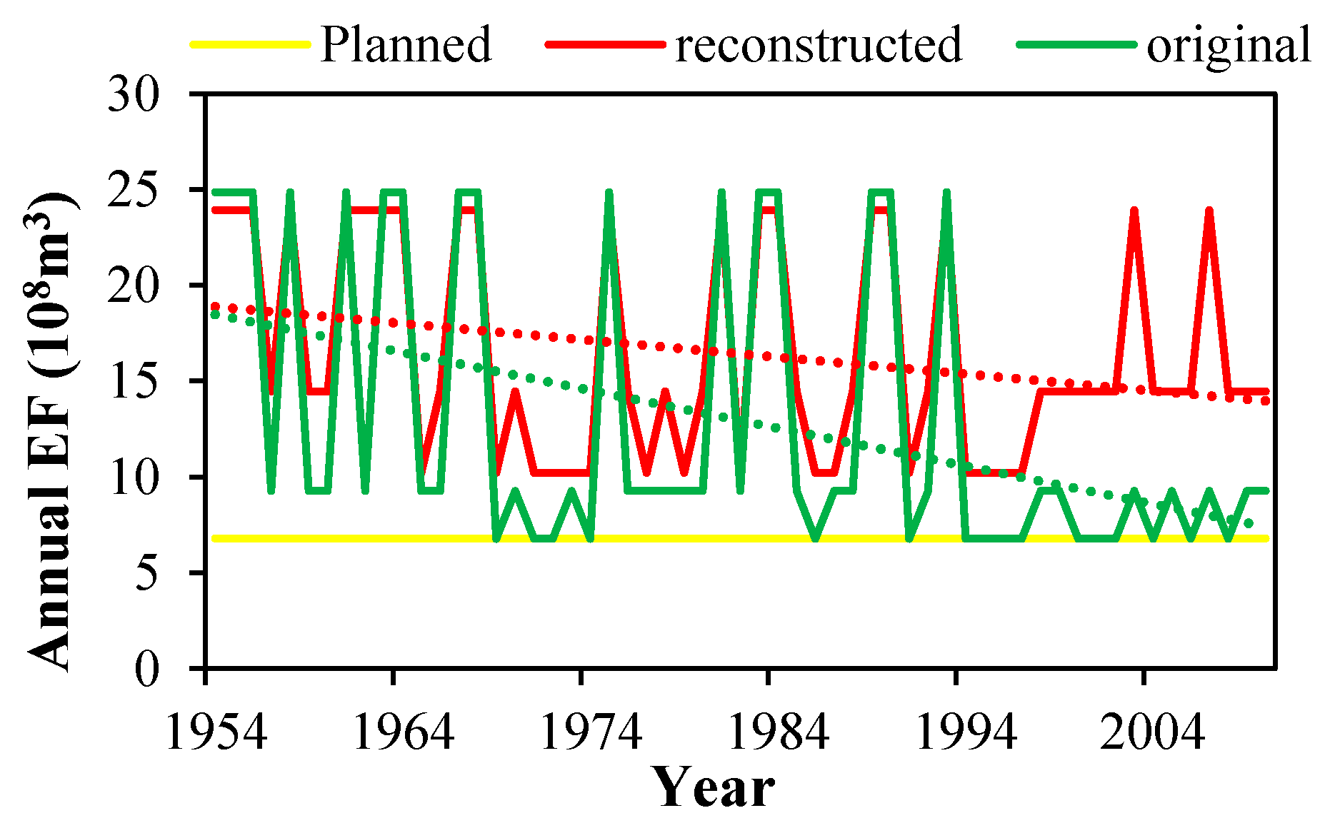
The annual EFs of the original and reconstructed streamflow are shown in Figure 10. This figure is quite revealing in several ways. First, the annual EF of the original and reconstructed streamflow are larger than the annual planned EF, both of which would make for more adequate protection of riverine ecosystems. Second, both of the annual EFs are almost consistent before the change point; however, there was a significant difference after the change point, and the EF of the original streamflow can efficiently generate realistic EF prescriptions under non-stationary conditions. Finally, the annual EF of the original streamflow shows a clear decreasing trend; however, it is not obvious in the annual EF of the reconstructed streamflow. It is indicated that the EF of the reconstructed streamflow is more sustainable for protection of the ecosystem because it will not lower the standards of ecological protection under the context of non-stationarity, and it provides a reasonable assessment for protection based upon historical information of riverine ecosystems.
5. Evaluation of Inter- and Intra-Annual Streamflow Characteristics
5.1. Evaluation of Inter-Annual Streamflow Characteristics
For the POD of the Jialing to Han River IBWT Project, the calculated and planned EFs were used as the constraints of the diverted process. Therefore, the streamflow is primarily assigned to satisfy the requirements of the EF and the residual runoff is assigned to divert in the POD. In this study, in order to comprehensively assess inter-annual streamflow characteristics with RVA, the original daily streamflow (1954–2010) is used as a pre-diversion series and the daily streamflow with diversion is used as a post-diversion series.
The different results of RVA are summarized in Table 2 (represented by Di). In the first group of magnitude of monthly river flow, the values of Di under the condition of calculated EF are all in the range of medium and low hydrological alteration. However, the values of Di under the condition of planned EF are almost half the number that are within the range of high hydrological alteration. The river hydrological regime has been significantly changed by the diversion. The high hydrological alteration is all in the dry season (e.g., January, February, March, and June) and the hydrological influence of diversion is more obvious in the low streamflow.
In the second group of magnitude of annual extreme water conditions, the 1-, 3- and 7-day minimum values of Di under the condition of calculated and planned EF are all in the range of high hydrological alteration, and the river hydrological regime was significantly changed. However, in comparison with the 30- and 90-day minimum values of Di under the condition of calculated EF, these values of Di under the condition of planned EF are also in the range of high hydrological alteration, which implies an increasing trend of the duration of low streamflow.
The third and fourth group of indicators further validated the results shown in the second group; that is, the duration of the minimum flow was significantly changed. Although, the number of minimum flow characteristics under the condition of calculated EF increased, the duration of the minimum flow was not affected.
In Group 5, the values of Di under the condition of calculated and planned EF are all in the range of medium to high hydrological alteration, but the values of Di under the condition of planned EF are more obviously changed by the diversion. Finally, the comprehensive alterations of the indicators are 45% and 64%, respectively, which shows that the calculated EF is more beneficial to protect the riverine ecosystem of the water transfer area.
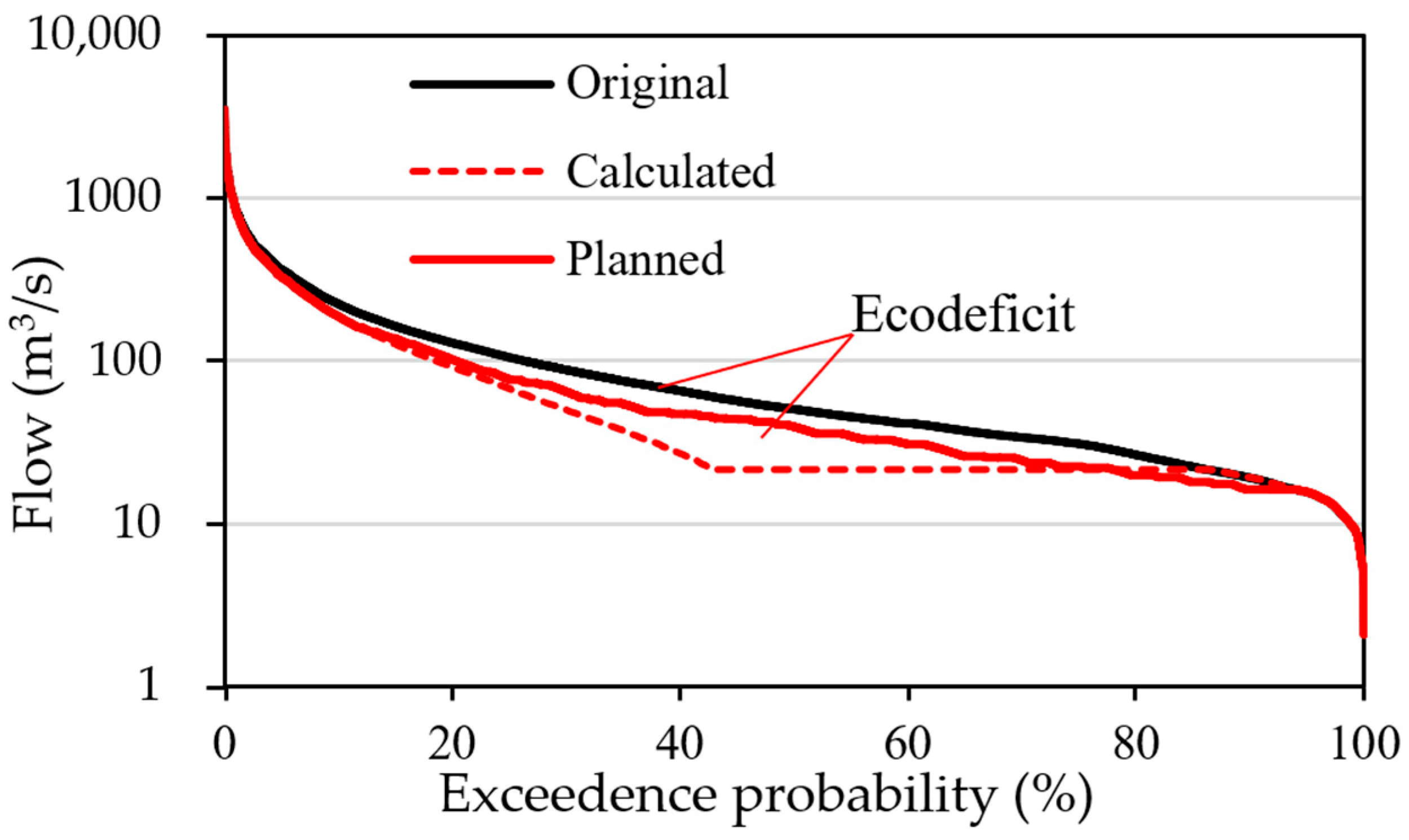
Figure 11 shows the flow duration curves (FDCs) between pre- and post-diversion series with different EFs. It can be seen from Figure 11 that the FDC of post-diversion streamflow with the calculated EF is approximately consistent with the FDC of pre-diversion streamflow. However, the FDC of post-diversion streamflow with planned EF, compared with the FDC of pre-diversion streamflow, was obviously changed by the diversion in the POD. And the eco-deficit of post-diversion streamflow in the planned EF is more serious, which has a more negative impact on riverine ecosystems.
5.2. Evaluation of Intra-Annual Streamflow Characteristics
Six indicators of intra-annual variation were calculated, and the average values are listed in Table 3. The box-plot of this indicator is displayed in Figure 12, which shows the difference of the intra-annual streamflow variability for the pre- and post-diversion series with different EFs. Through a comparison of the three calculated values under different coefficients, almost all the indicators of post-diversion are larger than those of the pre-diversion, i.e., all the indicators show obvious intra-annual variation in streamflow. The non-uniformity coefficient with a different EF increased by 7% and 16%, respectively, which indicates that monthly streamflow fluctuates more, and tends to be more uneven throughout the year after diversion. The distribution of Cn values with planned EF are more dispersed, the extreme values tend to increase, and the streamflow characteristics were completely changed by the diversion. The Cc and Cd values with different EFs are relatively stable, showing only a small increase. However, the values in the planned EF also showed a more dispersed distribution, and the extreme value increased. The Cp values show a significant increase under the condition of the calculated EF, which shows that the monthly streamflow after diversion is more uniform throughout the year. The Cr values with different EFs increased significantly. However, the increase in the calculated EF is greater, because the calculated EF is smaller than the planned EF in the dry season. Therefore, the water quantity of diversion with the calculated EF is greater in the dry season. The Ca values have little variance in three kinds of streamflow conditions, and the distribution is approximately consistent, which indicates that the relative variance between the extreme flow is relatively small, because the quantity of water diversion is only a small proportion of streamflow.
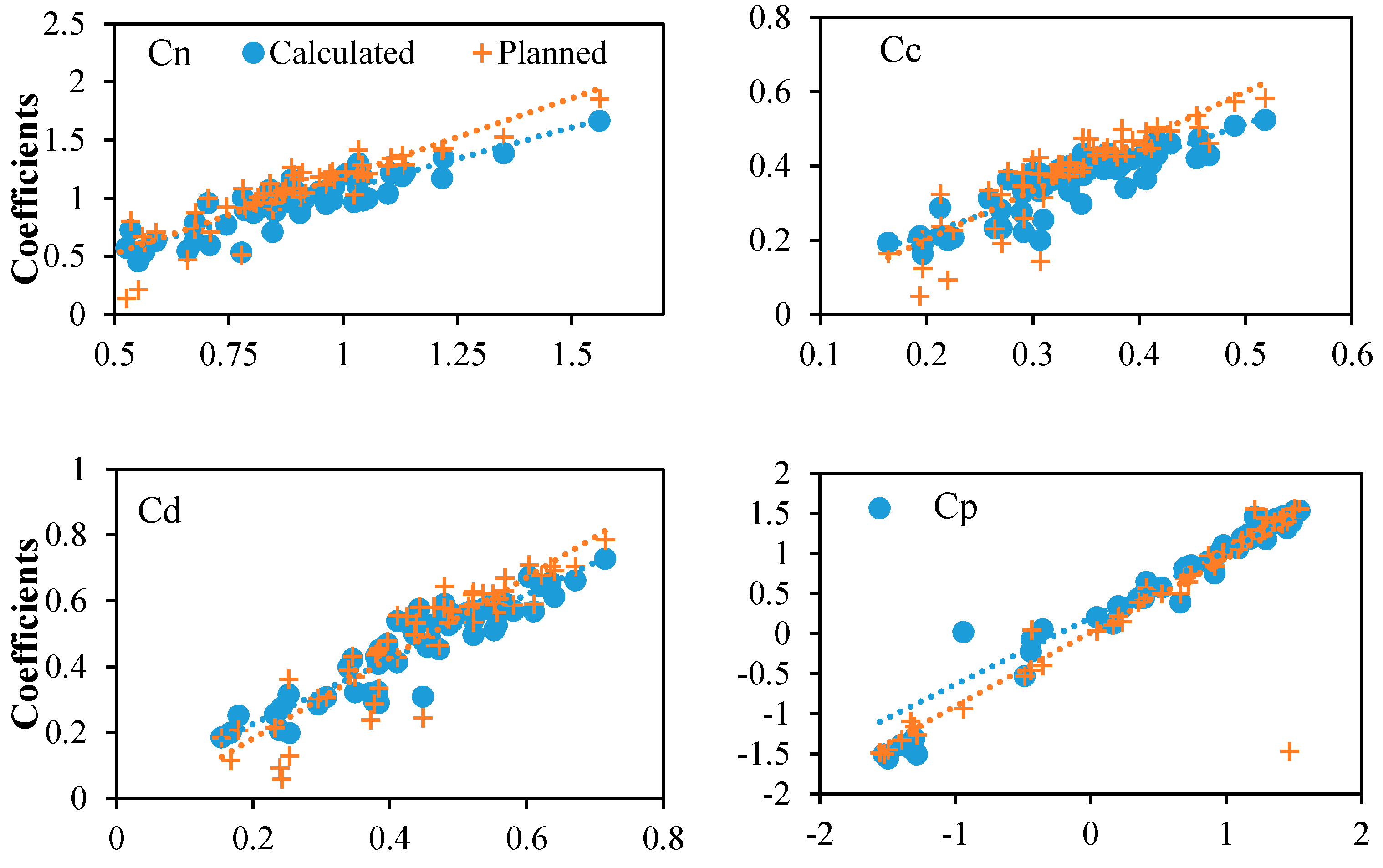
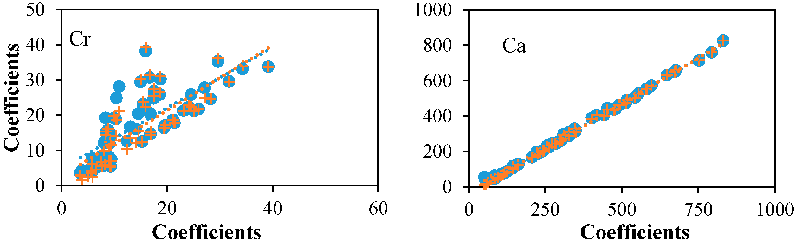
The correlations between the indices of intra-annual variations of streamflow in post-diversion with different EFs are analyzed; the results are illustrated in Figure 13. It can be observed from Figure 13 that almost all of these indices have a strong correlation, and there is also a great variance between the correlations of indicators, which indicates that the impacts of diversion on different indicators are not the same. In all correlation indices, the correlation of Cr is weakest, and the correlation of Ca is strongest, reaching a 99% confidence level. The result illustrates that the selected different criteria for the conservation of riverine ecosystems can have significantly different consequences, if we only focus on the protection of certain objectives that will inevitably affect other aspects. Note that most of the current studies of the assessment of EF are targeted at specific species and targets, which is not enough for the healthy and sustainable development of riverine ecosystems. Therefore, in future studies, it is necessary to synthesize all the protection objectives and to establish a comprehensively unified metric.
6. Conclusions
A comprehensive framework for assessing the EF was proposed in this study, which incorporates the inter- and intra-annual streamflow variability, and reconstructs the non-stationary streamflow to a stationary conditions. The Jialing to Han River IBWT Project was used to demonstrate the rationality and availability of the framework. Three subjects are pursued as follows:
First, the Mann-Kendall test method and the heuristic segmentation method were adopted to identify the change points. Based on the results of the two reasonable methods, the trend of decreasing of the annual streamflow data at the POD is obvious, and the change point of 1994 was observed. Second, the data homogeneity was achieved by processing data from the post-impact series in an additive procedure. The results reveal that the original streamflow series effectively eliminated the non-stationary components, and the reconstructed streamflow series ensure the consistency of the historical streamflow. Third, the inter- and intra-annual streamflow variability are incorporated by using SPI to identify the wet, normal, and dry years, and the percent of flow approach is applied to calculate the EF of the reconstructed streamflow series for the different water years. The calculated EF was applied to the Jialing to Han River IBWT Project. The results indicate that incorporating the inter- and intra-annual variability would further upgrade the ecosystem fitness and stability, and the water diversion with the calculated EF is more effective protection of riverine ecosystem in POD.
Traditional approaches to EF management are either too simple, which do not fully utilize the existing streamflow information, or they are too complex to require extensive site-specific data and expensive modelling, but many regions do not have such knowledge. Our technique can be applied to a wide range of instream flow management, and there is more comprehensive protection of riverine ecosystem, in particular, it is more applicable to instream flow management under the influence of climate change and human activities. An important question for future studies is to incorporate a component for real-time predictions of the water year types for the proposed method to be used as an effective management tool.
Author Contributions
Q.H. and S.H. proposed the idea of this paper; S.H. guided the writing and analyzing work; K.R. did the calculation work and wrote the manuscript; H.W. and G.L. commented on and revised the manuscript.
Funding
This research was jointly funded by the National Key Research and Development Program of China (grant number 2017YFC0405900), the National Natural Science Foundation of China (grant number 51709221), the Planning Project of Science and Technology of Water Resources of Shaanxi (grant numbers 2015slkj-27 and 2017slkj-19), and the Open Research Fund of State Key Laboratory of Simulation and Regulation of Water Cycle in River Basin (China Institute of Water Resources and Hydropower Research, grant number IWHR-SKL-KF201803.
Conflicts of Interest
The authors declare no conflicts of interest
References
- Vörösmarty, C.J.; Mcintyre, P.B.; Gessner, M.O.; Dudgeon, D.; Prusevich, A.; Green, P.; Glidden, S.; Bunn, S.E.; Sullivan, C.A.; Liermann, C.R.; et al. Global threats to human water security and river biodiversity. Nature 2010, 467, 555–561. [Google Scholar] [CrossRef] [PubMed] [Green Version]
- Wohl, E.; Angermeier, P.L.; Bledsoe, B.; Kondolf, G.M.; MacDonnell, L.; Merritt, D.M.; Palmer, M.A.; Poff, N.L.; Tarboton, D. River restoration. Water Resour. Res. 2005, 41, W10301. [Google Scholar] [CrossRef]
- Magilligan, F.J.; Nislow, K.H. Changes in hydrologic regime by dams. Geomorphology 2005, 71, 61–78. [Google Scholar] [CrossRef]
- Olden, J.D.; Naiman, R.J. Incorporating thermal regimes into environmental flows assessments: Modifying dam operations to restore freshwater ecosystem integrity. Freshwater Biol. 2010, 55, 86–107. [Google Scholar] [CrossRef]
- Ashraf, F.B.; Haghighi, A.T.; Marttila, H.; Kløve, B. Assessing impacts of climate change and river regulation on flow regimes in cold climate: A study of a pristine and a regulated river in the sub-arctic setting of Northern Europe. J. Hydrol. 2016, 542, 410–422. [Google Scholar] [CrossRef]
- Poff, L.R.; Allan, J.D.; Bain, M.B.; Karr, J.R.; Prestegaard, K.L.; Richter, B.D.; Sparks, R.E.; Stromberg, J.C. The natural flow regime. Bioscience 1997, 47, 769–784. [Google Scholar] [CrossRef]
- Lytle, D.A.; Poff, N.L. Adaptation to natural flow regimes. Trends Ecol. Evol. 2004, 19, 94–100. [Google Scholar] [CrossRef] [PubMed]
- Arthington, A.H.; Bunn, S.E.; Poff, N.L.; Naiman, R.J. The challenge of providing environmental flow rules to sustain river ecosystems. Ecol. Appl. 2006, 16, 1311–1318. [Google Scholar] [CrossRef]
- Poff, L.R.; Tokar, S.; Johnson, P. Stream hydrological and ecological responses to climate change assessed with an artificial neural network. Limnol. Oceanogr. 1996, 41, 857–863. [Google Scholar] [CrossRef] [Green Version]
- Poff, L.R.; Matthews, J.H. Environmental flows in the Anthropocence: Past progress and future prospects. Curr. Opin. Environ. Sustain. 2013, 5, 667–675. [Google Scholar] [CrossRef]
- Piniewski, M.; Laizé, C.L.; Acreman, M.C.; Okruszko, T.; Schneider, C. Effect of climate change on environmental flow indicators in the Narew basin, Poland. J. Environ. Qual. 2014, 43, 155. [Google Scholar] [CrossRef] [PubMed] [Green Version]
- Arthington, A.H.; Kennen, J.G.; Stein, E.D.; Webb, J.A. Recent advances in environmental flows science and water management—Innovation in the Anthropocene. Freshw. Biol. 2018, 00, 1–13. [Google Scholar] [CrossRef]
- Smakhtin, V.; Anputhas, M. An Assessment of Environmental Flow Requirements of Indian River Basins; IWMI International Water Management Institute: Colombo, Sri Lanka, 2009; pp. 13–23. [Google Scholar]
- Poff, N.L.; Brown, C.M.; Grantham, T.E.; Matthews, J.H.; Palmer, M.A.; Spence, C.M.; Wilby, R.L.; Haasnoot, M.; Mendoza, G.F.; Dominique, K.C.; et al. Sustainable water management under future uncertainty with eco-engineering decision scaling. Nat. Clim. Chang. 2016, 6, 25–34. [Google Scholar] [CrossRef] [Green Version]
- Shiau, J.T.; Wu, F.C. Pareto-optimal solutions for environmental flow schemes incorporating the intra-annual and interannual variability of the natural flow regime. Water Resour. Res. 2007, 43, 813–816. [Google Scholar] [CrossRef]
- Jager, H.I.; Smith, B.T. Sustainable reservoir operation: Can we generate hydropower and preserve ecosystem values? River Res. Appl. 2010, 24, 340–352. [Google Scholar] [CrossRef]
- Richter, B.D.; Warner, A.T.; Meyer, J.L.; Lutz, K. A collaborative and adaptive process for developing environmental flow recommendations. River Res. Appl. 2006, 22, 297–318. [Google Scholar] [CrossRef]
- Hughes, D.A.; Desai, A.Y.; Birkhead, A.L.; Louw, D. A new approach to rapid, desktop-level, environmental flow assessments for rivers in South Africa. Int. Assoc. Sci. Hydrol. Bull. 2014, 59, 673–687. [Google Scholar] [CrossRef] [Green Version]
- Acreman, M.; Arthington, A.H.; Colloff, M.J.; Couch, C.; Crossman, N.D.; Dyer, F.; Overton, I.; Pollino, C.A.; Stewardson, M.J.; Young, W. Environmental flows for natural, hybrid, and novel riverine ecosystems in a changing world. Front. Ecol. Environ. 2016, 12, 466–473. [Google Scholar] [CrossRef] [Green Version]
- Poff, N.; Richter, B.; Arthington, A.; Bunn, S.; Naiman, J.R.; Kendy, E.; Acreman, M.; Apse, C.; Bledsoe, B.P.; Freeman, M.C.; et al. The ecological limits of hydrologic alteration (ELOHA): A new framework for developing regional environmental flow standards. Freshw. Biol. 2010, 55, 147–170. [Google Scholar] [CrossRef]
- Belmar, O.; Velasco, J.; Martinez-Capel, F. Hydrological classification of natural flow regimes to support environmental flow assessments in intensively regulated Mediterranean Rivers, Segura River Basin (Spain). Environ. Manag. 2011, 47, 992–1004. [Google Scholar] [CrossRef] [PubMed]
- Finn, M.; Jackson, S. Protecting indigenous values in water management: A challenge to conventional environmental flow assessments. Ecosystems 2011, 14, 1232–1248. [Google Scholar] [CrossRef]
- Buchanan, C.; Moltz, H.L.N.; Haywood, H.C.; Palmer, J.B.; Griggs, A.N. A test of The Ecological Limits of Hydrologic Alteration (ELOHA) method for determining environmental flows in the Potomac River basin, USA. Freshw. Biol. 2013, 58, 2632–2647. [Google Scholar] [CrossRef]
- Mierau, D.W.; Trush, W.J.; Rossi, G.J.; Carah, J.K.; Clifford, M.O.; Howard, J.K. Managing diversions in unregulated streams using a modified percent-of-flow approach. Freshw. Biol. 2018, 63, 752–768. [Google Scholar] [CrossRef]
- King, A.J.; Gawne, B.; Beesley, L.; Koehn, J.D.; Nielsen, D.L.; Price, A. Improving ecological response monitoring of environmental flows. Environ. Manag. 2015, 55, 991–1005. [Google Scholar] [CrossRef] [PubMed]
- Fang, W.; Huang, S.Z.; Huang, G.H.; Huang, Q.; Wang, H.; Wang, L.; Zhang, Y.; Li, P.; Ma, L. Copulas-based risk analysis for inter-seasonal combinations of wet and dry conditions under a changing climate. Int. J. Climatol. 2018, in press. [Google Scholar] [CrossRef]
- Poff, L.R. Beyond the natural flow regime? Broadening the hydro-ecological foundation to meet environmental flows challenges in a non-stationary world. Freshw. Biol. 2018, 63, 1011–1021. [Google Scholar] [CrossRef]
- Liu, S.Y.; Huang, S.Z.; Xie, Y.Y.; Wang, H.; Leng, G.Y.; Huang, Q.; Wei, X.T.; Wang, L. Identification of the non-stationarity of floods: Changing patterns, causes, and implications. Water Resour. Manag. 2018, in press. [Google Scholar] [CrossRef]
- Liu, S.Y.; Huang, S.Z.; Xie, Y.Y.; Wang, H.; Huang, Q.; Leng, G.Y.; Li, P.; Wang, L. Spatial-temporal changes in vegetation cover in a typical semi-humid and semi-arid region in China: Changing patterns, causes and implications. Ecol. Indic. 2019, 98, 462–475. [Google Scholar] [CrossRef]
- Meng, E.H.; Huang, S.Z.; Huang, Q.; Fang, W.; Wu, L.Z.; Wang, L. A robust method for non-stationary streamflow prediction based on improved EMD-SVM model. J. Hydrol. 2019, in press. [Google Scholar] [CrossRef]
- Acreman, M.C.; Overton, I.C.; King, J.; Wood, P.J.; Cowx, I.G.; Dunbar, M.J.; Young, W.J.; Kendy, E. The changing role of ecohydrological science in guiding environmental flows. Int. Assoc. Sci. Hydrobiol. Bull. 2014, 59, 433–450. [Google Scholar] [CrossRef] [Green Version]
- Dhanya, C.T.; Kumar, A. Making a case for estimating environmental flow under climate change. Curr. Sci. 2015, 109, 1019–1020. [Google Scholar]
- Rodríguez, R.A.; Herrera, A.M.A.; Santander, J.; Miranda, J.V.; Perdomo, M.E.; Ángel, Q.; Riera, R.; Fath, B.D. From a stationary to a non-stationary ecological state equation: Adding a tool for ecological monitoring. Ecol. Modell. 2016, 320, 44–51. [Google Scholar] [CrossRef]
- Fang, W.; Huang, S.Z.; Ren, K.; Huang, Q.; Huang, G.H.; Cheng, G.H.; Li, K.L. Examining the applicability of different sampling techniques in the development of decomposition-based streamflow forecasting models. J. Hydrol. 2019, in press. [Google Scholar] [CrossRef]
- Liu, Q.; Yu, H.; Liang, L.; Ping, F.; Xia, X.; Mou, X.; Liang, J. Assessment of ecological instream flow requirements under climate change Pseudorasbora parva. Int. J. Environ. Sci. Technol. 2016, 14, 1–12. [Google Scholar] [CrossRef]
- Huang, S.; Chang, J.; Huang, Q.; Wang, Y.; Chen, Y. Calculation of the instream ecological flow of the Wei River Based on hydrological variation. J. Appl. Math. 2014, 11, 1–9. [Google Scholar] [CrossRef]
- Huang, S.Z.; Chang, J.X.; Huang, Q.; Chen, Y. Monthly streamflow prediction using modified EMD-based support vector machine. J. Hydrol. 2014, 511, 764–775. [Google Scholar] [CrossRef]
- Liang, W.; Bai, D.; Wang, F.; Fu, B.; Yan, J.; Wang, S.; Yang, Y.; Long, D.; Feng, M. Quantifying the impacts of climate change and ecological restoration on streamflow changes based on a Budyko hydrological model in China’s Loess Plateau. Water Resour. Res. 2015, 51, 6500–6519. [Google Scholar] [CrossRef]
- Yan, T.; Bai, J.; Yi, A.L.Z.; Shen, Z. SWAT-Simulated streamflow responses to climate variability and human activities in the Miyun Reservoir Basin by considering streamflow components. Sustainability 2018, 10, 941. [Google Scholar] [CrossRef]
- Chang, J.; Wang, Y.; Istanbulluoglu, E.; Bai, T.; Huang, Q.; Yang, D.; Huang, S. Impact of climate change and human activities on runoff in the Weihe River Basin, China. Quat. Int. 2015, 380–381, 169–179. [Google Scholar] [CrossRef]
- Guo, A.; Chang, J.; Liu, D.; Wang, Y.; Huang, Q.; Li, Y. Variations in the precipitation-runoff relationship of the Weihe River Basin. Hydrol. Res. 2017, 48, 295–310. [Google Scholar] [CrossRef]
- Du, J.; Shi, C.X. Effects of climatic factors and human activities on runoff of the Weihe River in recent decades. Quat. Int. 2012, 282, 58–65. [Google Scholar] [CrossRef]
- Huang, S.; Chang, J.; Huang, Q.; Chen, Y. Identification of abrupt changes of the relationship between rainfall and runoff in the Wei River Basin, China. Theor. Appl. Climatol. 2015, 120, 299–310. [Google Scholar] [CrossRef]
- Hamed, K.H.; Rao, A.R. A modified Mann-Kendall trend test for autocorrelated data. J. Hydrol. 1998, 204, 182–196. [Google Scholar] [CrossRef]
- Mann, H.B. Nonparametric test against trend. Econometrica 1945, 13, 245–259. [Google Scholar] [CrossRef]
- Huang, S.; Chang, J.; Huang, Q.; Chen, Y. Spatio-temporal changes and frequency analysis of drought in the Wei River Basin, China. Water Resour. Manag. 2014, 28, 3095–3110. [Google Scholar] [CrossRef]
- Shi, H.; Wang, G. Impacts of climate change and hydraulic structures on runoff and sediment discharge in the middle Yellow River. Hydrol. Processes 2015, 29, 3236–3246. [Google Scholar] [CrossRef] [Green Version]
- Pedro, B.G.; Plamen, I.C.; Luís, A.; Amaral, N. Scale invariance in the nonstationarity of human heart rate. Phys. Rev. Lett. 2001, 87, 168105. [Google Scholar] [CrossRef]
- Cleveland, R.B. STL: A seasonal-trend decomposition procedure based on loess. J. Off. Stat. 1990, 6, 3–33. [Google Scholar]
- Sanchezvazquez, M.J.; Nielen, M.; Gunn, G.J.; Lewis, F.I. Using seasonal-trend decomposition based on loess (STL) to explore temporal patterns of pneumonic lesions in finishing pigs slaughtered in England, 2005–2011. Prev. Vet. Med. 2012, 104, 65–73. [Google Scholar] [CrossRef] [PubMed] [Green Version]
- Theodosiou, M. Forecasting monthly and quarterly time series using STL decomposition. Int. J. Forecast. 2011, 27, 1178–1195. [Google Scholar] [CrossRef]
- Mckee, T.B.; Doesken, N.J.; Kleist, J. The relationship of drought frequency and duration to time scales. In Proceedings of the 8th Conference on Applied Climatology, Anaheim, CA, USA, 17–22 January 1993; pp. 179–184. [Google Scholar]
- Heim, R.R.J. A review of twentieth-century drought indices used in the United States. Bull. Am. Meteorol. Soc. 2002, 83, 1149–1165. [Google Scholar] [CrossRef]
- Hayes, M.J.; Svoboda, M.D.; Wilhite, D.A.; Vanyarkho, O.V. Monitoring the 1996 drought using the standardized precipitation index. Bull. Am. Meteorol. Soc. 1999, 80, 429–438. [Google Scholar] [CrossRef]
- Bonaccorso, B.; Bordi, I.; Cancelliere, A.; Rossi, G.; Sutera, A. Spatial variability of drought: An analysis of the SPI in Sicily. Water Resour. Manag. 2003, 17, 273–296. [Google Scholar] [CrossRef]
- Shiau, J.T. Fitting drought duration and severity with Two-Dimensional Copulas. Water Resour. Manag. 2006, 20, 795–815. [Google Scholar] [CrossRef]
- Raziei, T.; Saghafian, B.; Paulo, A.A.; Pereira, L.S.; Bordi, I. Spatial patterns and temporal variability of drought in western Iran. Water Resour. Manag. 2009, 23, 439–455. [Google Scholar] [CrossRef]
- Dubrovsky, M.; Svoboda, M.D.; Trnka, M.; Hayes, M.J.; Wilhite, D.A.; Zalud, Z.; Hlavinka, P. Application of relative drought indices in assessing climate-change impacts on drought conditions in Czechia. Theor. Appl. Climatol. 2009, 96, 155–171. [Google Scholar] [CrossRef]
- Svoboda, M.; LeComte, D.; Hayes, M.; Heim, R.; Gleason, K.; Angel, J.; Rippey, B.; Tinker, R.; Palecki, M.; Stooksbury, D.; et al. The Drought Monitor. Bull. Am. Meteorol. Soc. 2002, 83, 1181–1190. [Google Scholar] [CrossRef]
- Jowett, I.G.; Richardson, J. Habitat Use by New Zealand Fish and Habitat Suitability Models; NIWA Science Communication: Wellington, New Zealand, 2018; ISBN 987-0-478-23283-7. [Google Scholar]
- Richter, B.D.; Davis, M.M.; Apse, C.; Konrad, C. A presumptive standard for environmental flow protection. River Res. Appl. 2012, 28, 1312–1321. [Google Scholar] [CrossRef]
- Lynch, M.; Gabriel, W. Environmental tolerance. Am. Nat. 1987, 129, 283–303. [Google Scholar] [CrossRef] [Green Version]
- Yarnell, S.M.; Petts, G.E.; Schmidt, J.C.; Whipple, A.A.; Beller, E.E.; Dahm, C.N.; Goodwin, P.; Viers, J.H. Functional flows in modified Riverscapes: Hydrographs, Habitats and Opportunities. Bioscience 2015, 65, 963–972. [Google Scholar] [CrossRef]
- Davies, P.M.; Naiman, R.J.; Warfe, D.M.; Pettit, N.E.; Arthington, A.H.; Bunn, S.E. Flow–ecology relationships: Closing the loop on effective environmental flows. Mar. Freshw. Res. 2014, 65, 133–141. [Google Scholar] [CrossRef]
- Richter, B.; Baumgartner, J.; Wigington, R.; Braun, D. How much water does a river need? Freshw. Biol. 1997, 37, 231–249. [Google Scholar] [CrossRef]
- Yang, T.; Xu, C.Y.; Chen, X.; Singh, V.P.; Shao, Q.X.; Hao, Z.C. Assessing the impact of human activities on hydrological and sediment changes (1953–2000) in nine major catchments of the loess plateau, China. River Res. Appl. 2010, 26, 322–340. [Google Scholar] [CrossRef]
Figure 1.
Location of the inter basin water transfer project.

Figure 2.
The annual streamflow series in the POD.

Figure 3.
The results of change points with Mann-Kendall test method (a) and the heuristic segmentation method (b) in annual streamflow series in the POD.
Figure 3.
The results of change points with Mann-Kendall test method (a) and the heuristic segmentation method (b) in annual streamflow series in the POD.

Figure 4.
(a) Monthly streamflow series in the period 1954–2010, (b–d) seasonal, trend, and remainder series in the pre-impact series (1954–1993) and the post-impact series (1994–2010), respectively.
Figure 4.
(a) Monthly streamflow series in the period 1954–2010, (b–d) seasonal, trend, and remainder series in the pre-impact series (1954–1993) and the post-impact series (1994–2010), respectively.

Figure 5.
Reconstruction of monthly streamflow series (a) and annual streamflow series (b) in 1994–2010.
Figure 5.
Reconstruction of monthly streamflow series (a) and annual streamflow series (b) in 1994–2010.

Figure 6.
Determination of annual streamflow threshold for different water years.

Figure 7.
Annual hydrographs of mean monthly flow for different water years.

Figure 8.
The results of the calculated monthly EF for different water years of the reconstructed series.
Figure 8.
The results of the calculated monthly EF for different water years of the reconstructed series.

Figure 9.
The results of the calculated monthly EF for different water years of the reconstructed and original series.
Figure 9.
The results of the calculated monthly EF for different water years of the reconstructed and original series.

Figure 10.
The annual EF of the reconstructed and original series.

Figure 11.
The flow duration curves (FDC) between pre- and post-diversion streamflow series with different EFs.
Figure 11.
The flow duration curves (FDC) between pre- and post-diversion streamflow series with different EFs.

Figure 12.
The difference of the intra-annual streamflow variability for the pre- and post-diversion series with different EFs.
Figure 12.
The difference of the intra-annual streamflow variability for the pre- and post-diversion series with different EFs.

Figure 13.
Correlation coefficients of intra-annual variability between pre-diversion and post-diversion with different EF.
Figure 13.
Correlation coefficients of intra-annual variability between pre-diversion and post-diversion with different EF.


Table 1.
The results of the calculated monthly EF of different water years.
| Water Years | Monthly EF (m3/s) | |||||||||||
|---|---|---|---|---|---|---|---|---|---|---|---|---|
| Jan | Feb | Mar | Apr | May | Jun | Jul | Aug | Sept | Oct | Nov | Dec | |
| Wet | 22.6 | 22.2 | 26.0 | 47.4 | 44.6 | 44.2 | 127.9 | 138.9 | 161.2 | 151.1 | 76.8 | 48.6 |
| Normal | 16.3 | 16.3 | 23.8 | 42.4 | 44.0 | 25.6 | 59.3 | 86.5 | 71.7 | 73.6 | 55.6 | 35.9 |
| Dry | 18.1 | 17.6 | 19.4 | 47.3 | 58.0 | 25.6 | 40.7 | 32.9 | 46.0 | 33.0 | 30.9 | 19.9 |
Table 2.
The 32 IHA parameters for the pre- and post-diversion series with the different EF.
| Indicator | Calculated EF | Planned EF | ||||
|---|---|---|---|---|---|---|
| Medians (m3/s) | Di (%) | Medians (m3/s) | Di (%) | |||
| Pre | Post | Pre | Post | |||
| Group 1: Magnitude of monthly river flow | ||||||
| January | 27.4 | 18.1 | 12.1 | 27.4 | 21.6 | 101.7 |
| February | 28 | 17.6 | 12.1 | 28 | 21.6 | 101.7 |
| March | 34.6 | 23.8 | 29 | 34.6 | 21.6 | 74.1 |
| April | 61.3 | 46.7 | 19 | 61.3 | 24 | 63.8 |
| May | 64.1 | 44.6 | 3.4 | 64.1 | 24.1 | 32.8 |
| June | 58.3 | 28.5 | 37.9 | 58.3 | 21.6 | 69 |
| July | 104 | 76.4 | 8.6 | 104 | 64 | 1.7 |
| August | 91.4 | 86.5 | 6.9 | 91.4 | 66.5 | 6.9 |
| September | 140.5 | 126.3 | 13.8 | 140.5 | 102.5 | 3.4 |
| October | 109 | 81.5 | 3.2 | 109 | 74.5 | 21.4 |
| November | 62.5 | 55.5 | 19 | 62.5 | 22.1 | 58.6 |
| December | 33.4 | 32 | 6.9 | 33.4 | 21.6 | 63.8 |
| Group 2: Magnitude of annual extreme water conditions | ||||||
| 1-day minimum | 17.9 | 16.3 | 96.6 | 17.9 | 18.1 | 101.7 |
| 3-day minimum | 18.0 | 16.3 | 96.6 | 18.0 | 18.7 | 106.9 |
| 7-day minimum | 19.6 | 16.3 | 101.7 | 19.6 | 19.9 | 106.9 |
| 30-day minimum | 25.0 | 17.1 | 12.1 | 25.0 | 21.4 | 91.4 |
| 90-day minimum | 30.1 | 18.5 | 3.4 | 30.1 | 21.6 | 86.2 |
| 1-day maximum | 1270.0 | 1300.0 | 24.1 | 1270.0 | 1230.0 | 34.5 |
| 3-day maximum | 880.7 | 864.3 | 13.8 | 880.7 | 842.8 | 8.6 |
| 7-day maximum | 668.3 | 643.4 | 24.1 | 668.3 | 634.6 | 19.0 |
| 30-day maximum | 329.5 | 298.4 | 27.6 | 329.5 | 291.6 | 37.9 |
| 90-day maximum | 208.9 | 196.7 | 3.4 | 208.9 | 173.1 | 6.9 |
| Base flow index | 0.2 | 0.2 | 69.0 | 0.2 | 0.2 | 58.6 |
| Group 3: Timing of annual extreme water conditions | ||||||
| Date of minimum | 62.0 | 30.0 | 60.7 | 62.0 | 185.0 | 55.8 |
| Date of maximum | 207.0 | 205.0 | 7.6 | 207.0 | 207.0 | 11.1 |
| Group 4: Frequency and duration of high and low pulses | ||||||
| Low pulse count | 5.0 | 4.0 | 72.0 | 5.0 | 7.0 | 67.1 |
| Low pulse duration | 5.5 | 8.0 | 1.7 | 5.5 | 7.5 | 1.7 |
| High pulse count | 8.0 | 7.0 | 29.4 | 8.0 | 8.0 | 32.4 |
| High pulse duration | 4.5 | 4.0 | 6.8 | 4.5 | 4.0 | 6.8 |
| Group 5: Rate and frequency of water-condition changes | ||||||
| Rise rate | 4.4 | 8.7 | 74.1 | 4.4 | 12.5 | 74.1 |
| Fall rate | 3.9 | 6.6 | 53.5 | 3.9 | 9.7 | 89.7 |
| Reversals | 92.0 | 65.0 | 90.2 | 92.0 | 62.5 | 90.2 |
| D0 = 45% | D0 = 64% | |||||
Table 3.
Average indicators of intra-annual streamflow variability of pre- and post-diversion with different EF.
Table 3.
Average indicators of intra-annual streamflow variability of pre- and post-diversion with different EF.
| Different Conditions | Average Indicators of Intra-Annual Variations of Streamflow | |||||
|---|---|---|---|---|---|---|
| Cn | Cc | Cd | Cp | Cr | Ca | |
| Original streamflow | 0.87 | 0.33 | 0.44 | 0.56 | 14.99 | 330.98 |
| Post-division (calculated EF) | 0.93 | 0.35 | 0.47 | 0.67 | 17.73 | 300.85 |
| Post-division (planned EF) | 1.01 | 0.38 | 0.48 | 0.54 | 16.67 | 297.74 |
© 2018 by the authors. Licensee MDPI, Basel, Switzerland. This article is an open access article distributed under the terms and conditions of the Creative Commons Attribution (CC BY) license (http://creativecommons.org/licenses/by/4.0/).
Share and Cite
MDPI and ACS Style
Ren, K.; Huang, S.; Huang, Q.; Wang, H.; Leng, G. Environmental Flow Assessment Considering Inter- and Intra-Annual Streamflow Variability under the Context of Non-Stationarity. Water 2018, 10, 1737. https://doi.org/10.3390/w10121737
AMA Style
Ren K, Huang S, Huang Q, Wang H, Leng G. Environmental Flow Assessment Considering Inter- and Intra-Annual Streamflow Variability under the Context of Non-Stationarity. Water. 2018; 10(12):1737. https://doi.org/10.3390/w10121737
Chicago/Turabian StyleRen, Kang, Shengzhi Huang, Qiang Huang, Hao Wang, and Guoyong Leng. 2018. "Environmental Flow Assessment Considering Inter- and Intra-Annual Streamflow Variability under the Context of Non-Stationarity" Water 10, no. 12: 1737. https://doi.org/10.3390/w10121737
Note that from the first issue of 2016, this journal uses article numbers instead of page numbers. See further details here.