A Bias Correction Method for Rainfall Forecasts Using Backward Storm Tracking


School of Civil, Environmental and Architectural Engineering, College of Engineering, Korea University, Seoul 02841, Korea
*
Author to whom correspondence should be addressed.
Water 2018, 10(12), 1728; https://doi.org/10.3390/w10121728
Submission received: 23 October 2018
/
Revised: 19 November 2018
/
Accepted: 22 November 2018
/
Published: 26 November 2018
(This article belongs to the Section Hydrology)
Abstract
:This study proposes a new method to estimate the bias correction ratio for the rainfall forecast to be used as input for a flash flood warning system. This method requires a backward tracking to locate where the forecasted storm is at the present time, and the bias correction ratio is estimated at the tracked location, not at the warning site. The proposed method was applied to the rainfall forecasts provided by the Korea Meteorological Administration. A total of 300 warning sites considered in the flash flood warning system for mountain regions in Korea (FFWS-MR) were considered as study sites, along with four different storm events in 2016. As a result, it was confirmed that the proposed method provided more reasonable results, even in the case where the number of rain gauges was small. Comparison between the observed rain rate and the corrected rainfall forecasts by applying the conventional method and the proposed method also showed that the proposed method was superior to the conventional method.
1. Introduction
The concept of flash flood was proposed by the U.S. National Weather Service (NWS) in the 1970s [1,2]. The NWS defined a flash flood as a flood due to a fast-moving concentrated storm, with a rainfall depth of more than 100 mm within two hours in a small steep river basin of less than 100 km2. Flooding due to a sudden rise of water in upstream channels caused by a typhoon or dam break was also included in the flash flood definition. Similar definitions can also be found in Korea [3,4].
The most serious problem with a flash flood is that a general flood warning system based on rain gauge information may not issue a warning, as the runoff travel time is too short. The flash flood occurs within an hour after the rainfall. Too low a rain gauge density in those basins vulnerable to flash flood may be another problem that reduces the quality of warnings. In general, the rain gauge density is very low in mountainous basins. The same problem also exists in Korea [5].
Many studies have been devoted to this flash flood problem. For example, Sweeney et al. (1993) showed the usefulness of GIS applications to develop flash flood guidance for the Raccoon river catchment in Iowa [6], and Carpenter et al. (1999) proposed a method of determining the threshold runoff for several large regions including California, Iowa, and Oklahoma [7]. Bhaskar et al. (2000) proposed a flash flood index based on the characteristics of runoff hydrograph to be used as indicator for flash flood warning in Kentucky [8]. Mukhopadhyay et al. (2003) used Next-Generation Weather Radar (NEXRAD) data to predict the occurrence potential of flash flood at alluvial fans in Dona Ana County, New Mexico [9]. In addition, several studies were devoted to the flash flood problem in mountainous regions with sparse rain gauge stations, such as Colorado in the USA, the Alps in Italy, and Gredos in Spain [10,11,12,13]. In Korea, Shin et al. (2004) evaluated the use of the geomorphoclimatic unit hydrograph (GcIUH) to determine flash flood guidance [14], and Bae and Kim (2007) proposed a method to determine flash flood guidance considering the soil moisture condition [4]. The use of radar information is indispensable to overcome the problem of short runoff travel time. In fact, the data to be used for warning of flash floods are the very-short-term rainfall forecasts, produced with the input of radar information. Many models have been developed for this purpose. For example, the National Center for Atmospheric Research (NCAR) developed the Auto NowCaster (ANC) for forecasting convective storms [15]. Thunderstorm Identification, Tracking, Analysis and Nowcasting (TITAN) was also developed for nowcasting convective storms [16], which is being operated by the Bureau of Meteorology Research Center (BMRC) to produce 10- to 60-min forecasts every 10 min. The Japan Meteorological Administration (JMA) operates the Meso-Scale Model (MSM) [17,18], whose rainfall forecasts are provided in real time, and used by many government agencies and research centers. In Korea, the McGill Algorithm for Precipitation Nowcasting by Lagrangian Extrapolation (the so-called MAPLE) has been used in the past several years. Originally developed by Bellon and Austin (1978) [19], MAPLE derives the storm moving vector based on the variational echo tracking technique, and forecasts the storm location based on the semi-Lagrangian method [20,21,22,23]. Recently, NOAA (National Oceanic and Atmospheric Administration)’s Local Analysis and Prediction System (LAPS) was introduced in Korea, modified to be applied to the Korean Peninsula and surrounding region [24]. The LAPS is a meteorological assimilation tool that employs available observations, like radar, satellite, etc., to generate a three-dimensional information of atmospheric conditions. Recent studies also focused on updating the developed models [25,26], as well as the application of this newly available information [27,28,29].
Radar information, which is based on a remote sensing technique, intrinsically involves many different kinds of errors. For example, the adopted Z–R relationship may not be so flexible as to be tailored to each specific situation. It is well known that it frequently fails to correctly estimate extreme events. The radar beam propagation can also be partially or totally blocked by obstacles. Ground clutter is another source of error that adds disturbance to radar echoes [30,31,32,33]. Overall, these errors are divided into two types: one is randomness, while the other is bias. As randomness is more related to the condition of equipment, as well as the natural variability of the target process [34], once the information is collected, the most attention is given to bias correction. For the mean-field-bias correction of radar rainfall information, the method of direct comparison of radar information and ground information is generally used. The ratio of ground rain rate and radar rain rate is called the G/R ratio [35].
The same problems occur when using the rainfall forecast. Due to the errors involved in the input radar data, as well as the limitations of forecasting models, the rainfall forecast shows similar problems of randomness and bias. Practically, it is not easy to handle the randomness problem at the stage of utilizing the rainfall forecast. Thus, the focus is on the correction of bias. Exactly the same method, i.e., comparison of the rainfall forecast and the ground data, is applied to the rainfall forecast, but a somewhat different situation causes another problem to deteriorate the quality of bias correction. The difference in this case is that there exists a time gap between the rainfall forecast and ground data. As an example, the correction of the three-hour forecast is considered. A bias correction ratio is estimated at the present time by comparing the three-hour rainfall forecast made three hours before, and the ground data observed now. This bias correction ratio is then applied to the forecast three hours from now.
This temporal gap can be a serious problem, especially for fast moving storms. As the flash flood warning system covers some vulnerable small steep basins and not the entire country, the size of domain considered for correcting the rainfall forecast is not so large as for radar. That is, it is possible to have no rain or a low rain rate, as the storm has not arrived at the flash flood warning site. The bias correction ratio can be estimated to be too extreme. That is, the effect of randomness, as well as the bias involved in the rainfall forecast, can be too greatly amplified. An abnormal bias correction ratio can be estimated to result in extremely high or low correction of rainfall forecast. This problem has frequently been observed in the operation of the flash flood warning systems in Korea [36].
As a detour to overcome this problem, this study proposes a method of estimating the bias correction ratio where the storm was, not at the warning site. This method requires a backward tracking to locate where the forecasted storm at the warning site is at the present time. This backward tracking is like the comparison of the forecasted rainfall field over the warning site and the rainfall field at the present time, which is, in fact, used as input for generating the rainfall forecast. As the bias correction ratio is calculated where the storm is at the present time, it is expected to be more realistic and accurate to correct the bias of the rainfall forecast. Obviously, it is based on the assumption that the storm characteristics may not be much changed within a few hours. The proposed method is applied to the MAPLE rainfall forecasts provided by the Korea Meteorological Administration (KMA). The rainfall forecast from MAPLE is provided in the form of ASCII file, and composed of 1024 × 1024 grids with a resolution of 1 km × 1 km. Also, the Automatic Weather Station (AWS) rain gauge data are to be used for comparison purposes.
2. Methodology
2.1. Storm Tracking
The pathway of a storm can be determined by applying a storm tracking method. The storm tracking method provides information about the moving direction and velocity, which continuously changes in time. It is also possible to predict the future location of the storm using the derived information of the storm trajectory. Traditionally, storm tracking was done by analyzing the rain gauge data, but recently two-dimensional rainfall field derived by radar or satellite is generally analyzed. Both physical and statistical concepts are also considered in the derivation of motion field, such as the MAPLE based on the concept of Lagrangian persistence [20,23,37].
Early studies of storm tracking were done with the rain gauge data. For example, Huff (1967) derived isohyetal patterns of storms to analyze the uncertainty (i.e., the variance) of storm movement [38]. Clayton and Deacon (1971) proposed a storm tracking method based on the storm center determined as the center of mass [39]. Marshall (1980) introduced a statistical concept (i.e., the lag-correlation analysis) to derive the cross-correlation function of rain gauges to be used for the storm tracking [40], while Niemczynowicz (1987) applied the lag-correlation analysis to capture the characteristics of storm movement as well as their effect on runoff estimation [41].
Radar data were also used for storm tracking. Wilson (1966) derived and used the correlation structure of consecutive radar images for storm tracking [42], while Leese et al. (1971) analyzed the cross-correlation structure of radar data to estimate the storm moving velocity [43]. Austin and Bellon (1974) predicted the rainfall pattern using the velocity vector of rain rate field derived by analyzing radar images [44], and Rinehart and Garvey (1978) proposed a tracking of radar echoes with correlation (TREC) to do the six-hour-ahead forecasting of the rain rate field [45]. Hilst and Russo (1960) proposed a method based on pattern correlation [46]. In simple terms, the storm moves where the pattern correlation (i.e., similarity of storm shape) becomes the highest. As a short time period is concerned, it is assumed that the storm moves without any change in its shape. This study adopted this storm tracking method based on pattern correlation.
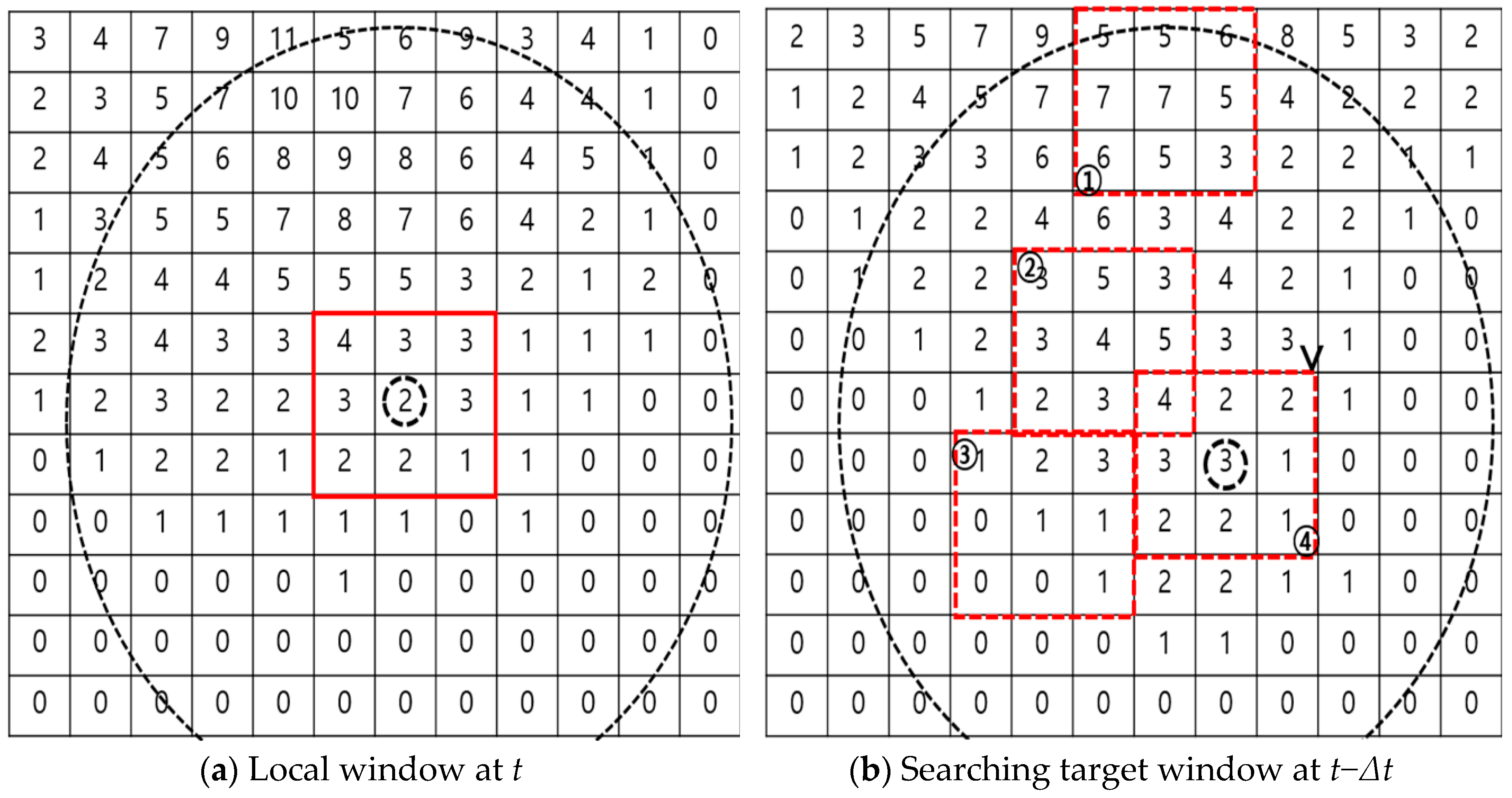
To do the storm tracking based on the pattern correlation coefficient, it is necessary to determine the size of window, and the range of storm tracking. Here, the window indicates the region where the pattern correlation coefficient is calculated, and the range indicates the boundaries within which the window moves. The size of window can vary depending on the size of a storm, and the range can be larger when the storm moving velocity is high. The pattern correlation coefficient is generally calculated for every possible location of windows inside the range. Figure 1a shows an example window within the range of calculation. Here, the shape of the window is assumed to be rectangular, and the range to be a circle. Within the range, the pattern correlation coefficient of each window is calculated, and compared to select the highest one. As an example, shown in Figure 1b, if the pattern correlation coefficient of window ④ is estimated to be the highest, then the storm is assumed to be located at the center of window ④ after Δt-hour.
The pattern correlation coefficient is calculated as follows:
where Tm,n is the forecasted rain rate at the location of (m, n), and at time t, and Um,n is the forecasted rain rate at the same location, but at time t−Δt. is the mean rain rate over the window at time t, and is the same, but at time t−Δt. The pattern correlation coefficient R has the value of (−1 to 1), and the pattern correlation is high when R is near −1 or +1, but low when R is near 0. That is, the pattern correlation coefficient −1 or +1 indicates that the patterns of rainfall field over the window at t−Δt and t are identical. Negative pattern correlation indicates that the spatial pattern of a storm is reversed, which may be due to the circulation of a storm.
The backward tracking in this study was done by division into three steps. The first step is to setup a window around the warning site (i.e., local window) over the forecasted rainfall field at the present time step; the second step is to locate the search domain in the forecasted rainfall field at the previous time step; and the third step is to find the most similar window (i.e., target window) within the search domain to the local window setup at the first step. The shape of the window was assumed to be rectangular, and its size was determined to be 20 km × 20 km, to consider the basin size of 300 flash flood warning sites. Their basin areas are all less than a few square kilometers. The size of the search domain should be much larger than that of the window, and it is also important to consider the storm velocity and the lead time for forecasting. In this study, the domain was assumed to be circular, and its radius was determined to be 50 km for the case where the lead time is one hour. In Korea, the mean speed of storm movement is known to be around 25–45 km/h [47]. For the longer lead time, the radius of the search domain should be larger. Finally, the target window is determined as that with the highest pattern correlation coefficient R.
2.2. Bias Correction Ratio
This study proposes a method of estimating the bias correction ratio where the storm was, not at the warning site. This method requires a backward tracking to locate where the forecasted storm at the warning site is at the present time. The bias correction ratio is estimated by comparing the forecasted rainfall field and the observed rainfall on the ground where the storm is at the present time.
The bias correction is a common procedure for the use of radar rainfall data. The so-called G/R ratio (the ratio estimated by dividing the ground rain rate by the radar rain rate) is used for correcting the mean-field-bias of radar rain rate [33,42]. It is generally estimated for a given region or basin, and sometimes a continuous field of G/R ratio is estimated to consider the possible variation in space. The G/R ratio is calculated as follows:
where G/R represents the G/R ratio, n is the number of data pairs, Gi represents the ground rain gauge rain rate, and Ri is the radar rain rate. If the G/R ratio is 1.0, it is assumed that no bias exists in the radar data. In general, the G/R ratio is estimated to be higher than 1, which indicates that the radar underestimates the rain rate.
Many studies have been done to use the G/R ratio for the correction of the mean-field-bias of radar rain rate. The first study was done by Wilson (1970) to derive and correct the mean-field-bias [42], and Brandes (1975) showed that the G/R ratio varies in space [48]. Lin (1989) showed that the G/R ratio varies storm by storm, also over time, even within the same storm event [49]. A Kalman filter has been applied to overcome this variation of the G/R ratio in time to real-time correct the radar rain rate [50,51,52]. Many studies also focused on the characteristics of the G/R ratio, as well as its accurate estimation [53,54].
2.3. Conventional and Proposed Method for Determining the Bias Correction Ratio
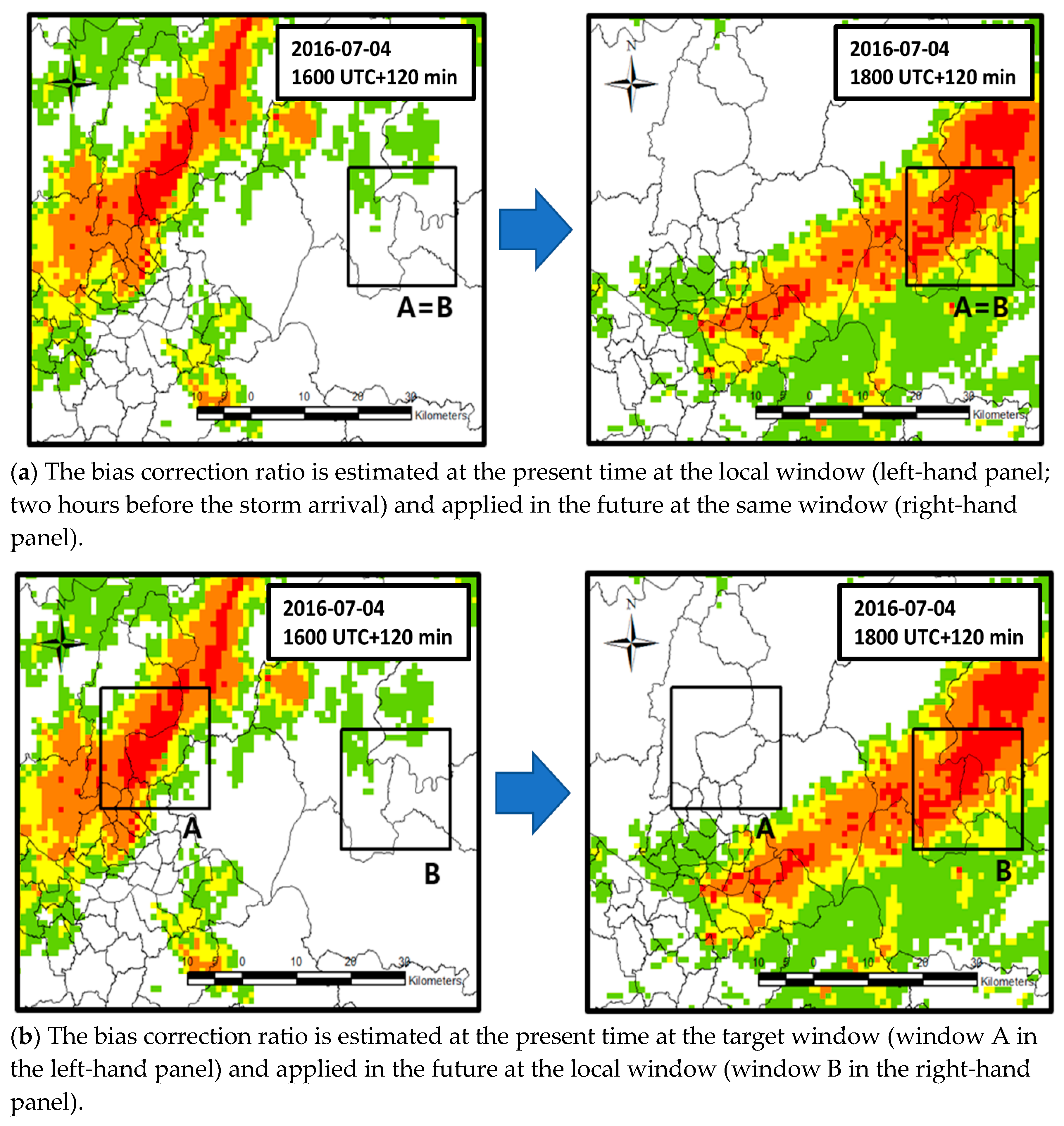
The bias correction for the rainfall forecast is also similar to that for the radar rainfall data. The bias correction ratio is estimated and applied where the rainfall forecast is applied. Figure 2a shows a schematic of the bias correction ratio estimation and application being used at present. That is, the window for estimating the bias correction ratio and the window for applying the bias correction ratio are identical. Assume that the rainfall is measured by ground rain gauges every hour, and the two-hour rainfall forecasting is made at the same time interval. Now the two-hour rainfall forecast shows that there will be a severe storm at an area ‘A = B’. Then, the two-hour rainfall forecasting made two hours ago is first compared with the rainfall data observed at present, to calculate the bias correction ratio. This bias correction ratio is then to be applied to the two-hour rainfall forecast made at present.
The method proposed in this study is to estimate the bias correction ratio where the storm was located, and apply it where the storm is forecasted to move. That is, the difference between the conventional and proposed method comes from whether considering the movement of storm or not. Under the same situation considered above, the bias correction ratio is first estimated at the location of the storm that will visit area ‘B’ after two hours. At this stage, it is important to locate window ‘A’, where the storm is located now (Figure 2b). This procedure can be rather complicated if the size of the window is small. It is also possible that the two-hour rainfall forecast at window ‘B’ does not contain the storm center. In this study, a backward tracking method based on the pattern correlation coefficient will be applied to find the location of window ‘A’. The bias correction ratio is then estimated at the location of window ‘A’. The bias correction ratio is then applied to the two-hour rainfall forecast, as shown in Figure 2b. That is, the bias correction ratio estimated at location ‘A’ at present is applied to the storm event that arrives at location ‘B’ after two hours.
3. Study Sites and Storm Events
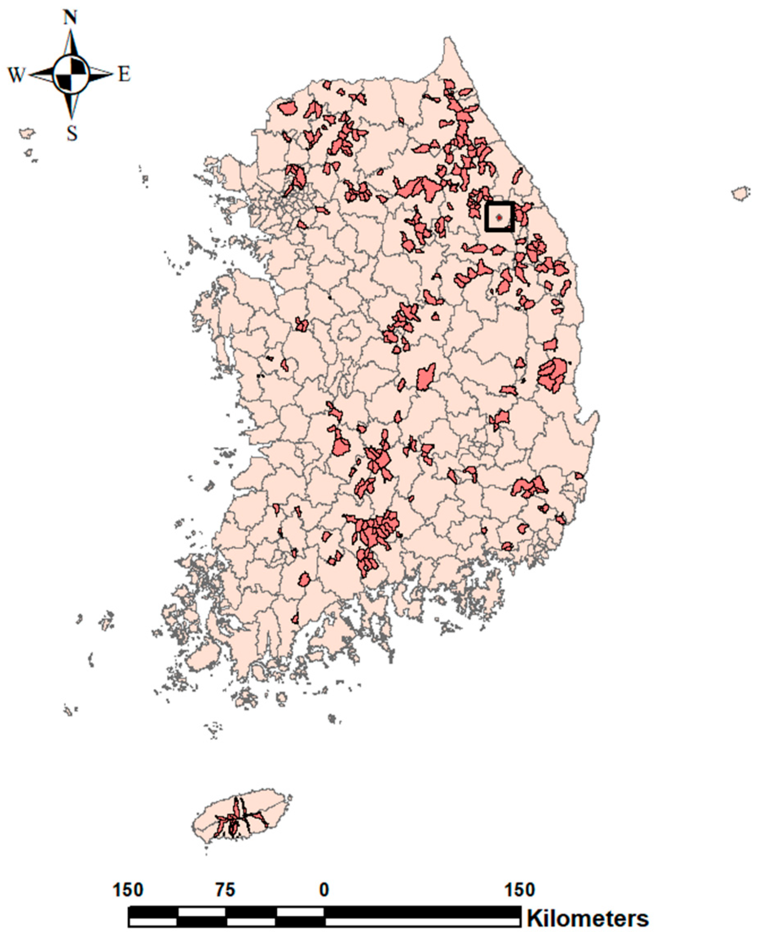
This study considered a total of 300 flash flood warning sites included in the Flash Flood Warning System for Mountainous Region developed by the National Disaster Management Institute (NDMI) in 2010 [36]. Those 300 locations are all tourist attractions during summer, and located at the exits of small mountainous basins (Figure 3). The sites are distributed over the entire South Korea, but are more concentrated in the eastern mountainous region. In this manuscript, the Ducsanggi Valley, one of the 300 warning sites located in the Gangwon Province, was considered as an example. The Ducsanggi Valley is a typical mountainous basin whose basin area is just 11.19 km2. The location of the Ducsanggi Valley is within the solid box in Figure 3.
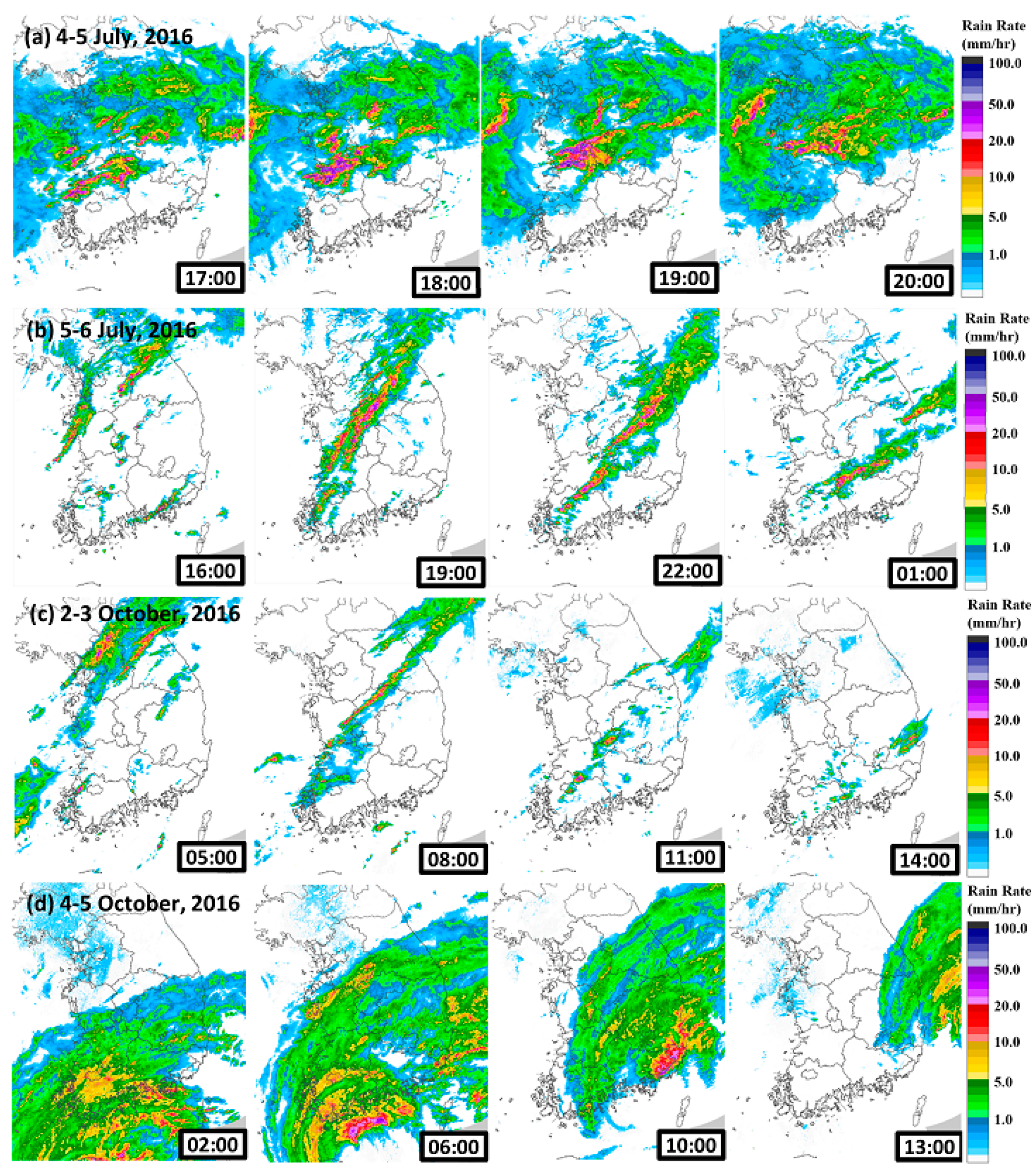
This study considered four storm events that occurred in 2016 (Table 1). Figure 4 shows the radar images (available at http://radar.kma.go.kr/) of these storms, which all satisfy the condition for flash flood. The first and second storm events all occurred during the monsoon season in Korea. Just after the first event passed the Korean Peninsula, the second event arrived at the western part of the Korean Peninsula. Most of the rainfall was concentrated in the middle of the Korean Peninsula, with a total depth of more than 200 mm, and the maximum rain rate of 34.5 mm/h was recorded at the Jeichun rain gauge station on 4 July. The second event had more impact in the eastern part of the Korean Peninsula, with total rainfall depth also of more than 200 mm, and the maximum rain rate of 57.1 mm/h recorded at the Wonju rain gauge station on 5 July. The third event was a convective storm that occurred on 2 October, which left some damage in the northern part of the Korean Peninsula. The maximum rain rate was 18.3 mm/h recorded at the Paju rain gauge station, and the total rainfall depth was more than 100 mm. The fourth storm event was typhoon Chaba, which left severe damage in several cities, including Pusan City and Ulsan City located in the southern part of the Korean Peninsula. Typhoon Chaba landed at Pusan City around 11:00 5 October, and after just one hour, it arrived at Ulsan City. The maximum rain rate was 98.3 mm/h, and the total rainfall depth was more than 300 mm. The return period was estimated to be longer than 100 years. In particular, the downtown area of Ulsan City was totally inundated during the storm.
This study also considered the one-, two-, and three-hour rainfall forecasts from MAPLE. MAPLE provides every hour rainfall forecasts up to 6 h at intervals of 10 min. In Korea, rainfall forecasts up to three hours are generally used for flash flood warning. In this part of the study, whenever the rain rate higher than 10 mm/h was forecasted near the flash flood warning sites, the backward storm tracking was done, and the bias correction ratio estimated.
4. Results
4.1. An Example Application to the Ducsanggi Valley
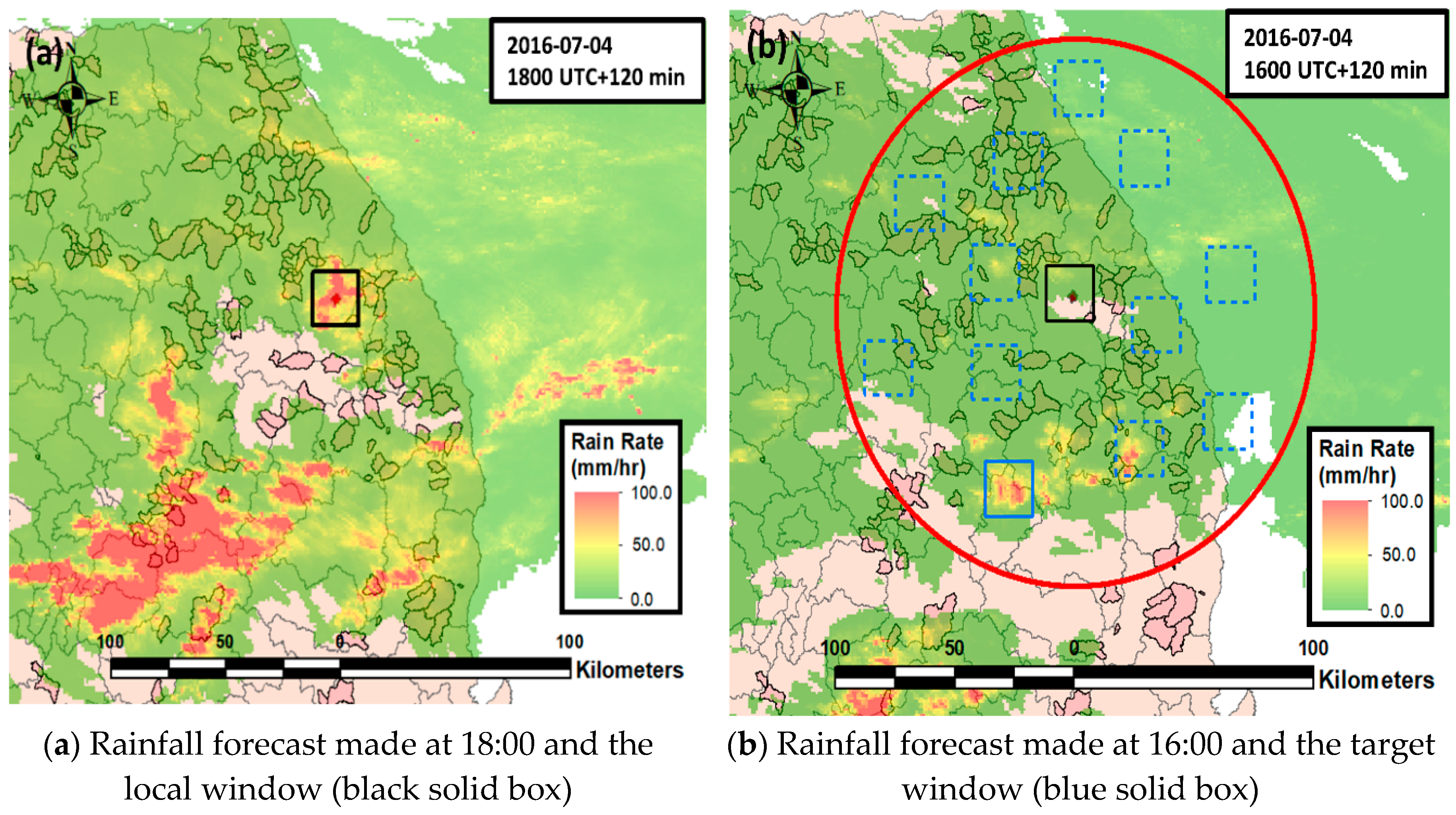
As mentioned earlier, the backward tracking was done by division into three steps. As the first step, a local window was setup around the warning site, in this example the Ducsanggi Valley, with the forecasted rainfall field. Figure 5a shows the two-hour rainfall forecast from MAPLE made at 18:00 4 July. Also, the box in the figure shows the local window setup for backward tracking. The shape of the local window was assumed to be rectangular with a size 20 km × 20 km. The size of the window was determined by considering the basin area of the warning sites, and the number of rain gauges. The biggest basin area among 300 warning sites is the 197 km2 of the Okkyo Valley, and three to five rain gauges are generally available with the 20 km × 20 km window area.
The next step is to determine the shape and size of the search domain around the local window. In this study, the shape of the search domain was determined to be a circle with a radius of 100 km, by considering the maximum storm velocity 50 km/h, and the forecasting lead time of two hours (Figure 5b). If longer lead time is considered, the search domain could be much larger.
Finally, the target window for estimating the bias correction ratio was located within the search domain, where the pattern correlation between the local window and the target window is the highest. As the search domain is not so large, a random search could be used, without the burden of searching time. Figure 5b shows the location of the final target window (solid line in blue color), whose pattern correlation was estimated to be 0.656.
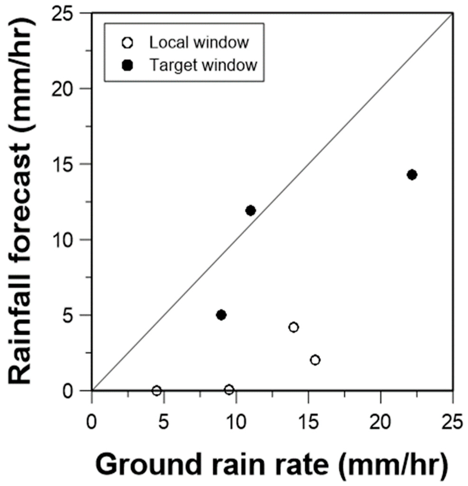
The forecasted rain rate is obviously different from that of rain gauges both in the local and target windows. In this example, the number of rain gauges available in the local window was four (Bukpyung, Imgye, Jungsun, and Hajang), and that in the target window was three (Yechun, Isan, and Dongro). In the conventional method, as the local window and the target window are identical, the bias correction ratio was estimated with the rain gauge data from four gauges in the local window. On the other hand, in the proposed method, the bias correction ratio was estimated in the target window, so the rain gauge data from three rain gauges in the target window were used to estimate the bias correction ratio. Figure 6 compares these two cases with the scatterplots of the forecasted rainfall and (observed) rain gauge rainfall data (two-hour rainfall forecast from MAPLE made at 16:00 4 July and hourly rainfall observed at 18:00 4 July).
In the case the forecasted and observed data are similar, more points are located around the one-to-one line. Also, the smaller extent to which the data are scattered around the mean indicates a consistent relationship between the forecasted and observed rainfall data. Figure 6 clearly shows that the case based on backward tracking provides a more consistent relationship between forecasted and observed data. Also, the slope is nearer to the one-to-one line to lead a reasonable bias correction ratio (i.e., 1.35). In the conventional method, many observed data were found to be too small, which forced the slope to move far away from the one-to-one line. As a result, the bias correction ratio was estimated to be very high (i.e., 6.96).
4.2. Overall Results
This study considered all the 300 warning sites for all four storm events from the beginning to the end. Whenever the rainfall forecast with 10 mm/h or higher was given at any of the warning sites, the backward tracking was done, and the bias correction ratio estimated. Also, in this part of the study, three different lead times of one hour, two hours, and three hours were considered, to evaluate the performance of the backward tracking and bias correction, depending on the lead time.
First, Table 2 summarizes the basic statistics of all the pattern correlations estimated every hour, and at every site available. As can be expected, the pattern correlation was, on average, higher for the lead time of one hour, and smaller for the lead time of three hours. However, this pattern was not so consistent in all storm events. In particular, no obvious difference could be detected between the lead times of one hour and two hours, and, in the fourth storm event, the pattern correlation for the lead time of three hours was estimated to be a bit higher than that of two hours. However, in all cases, the standard deviations were estimated to be about 0.1.
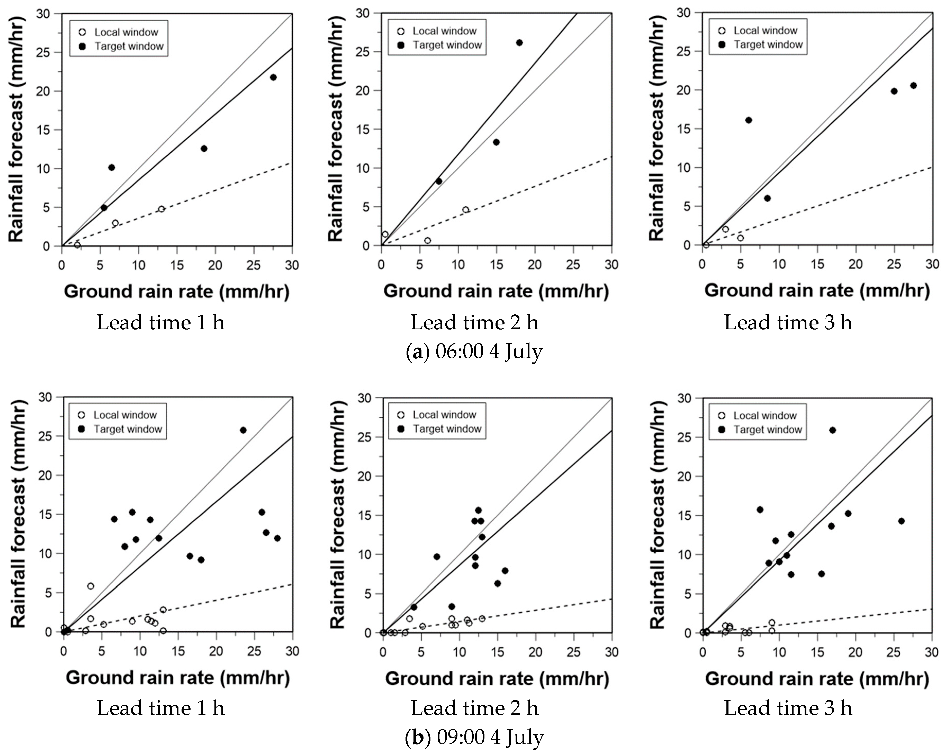
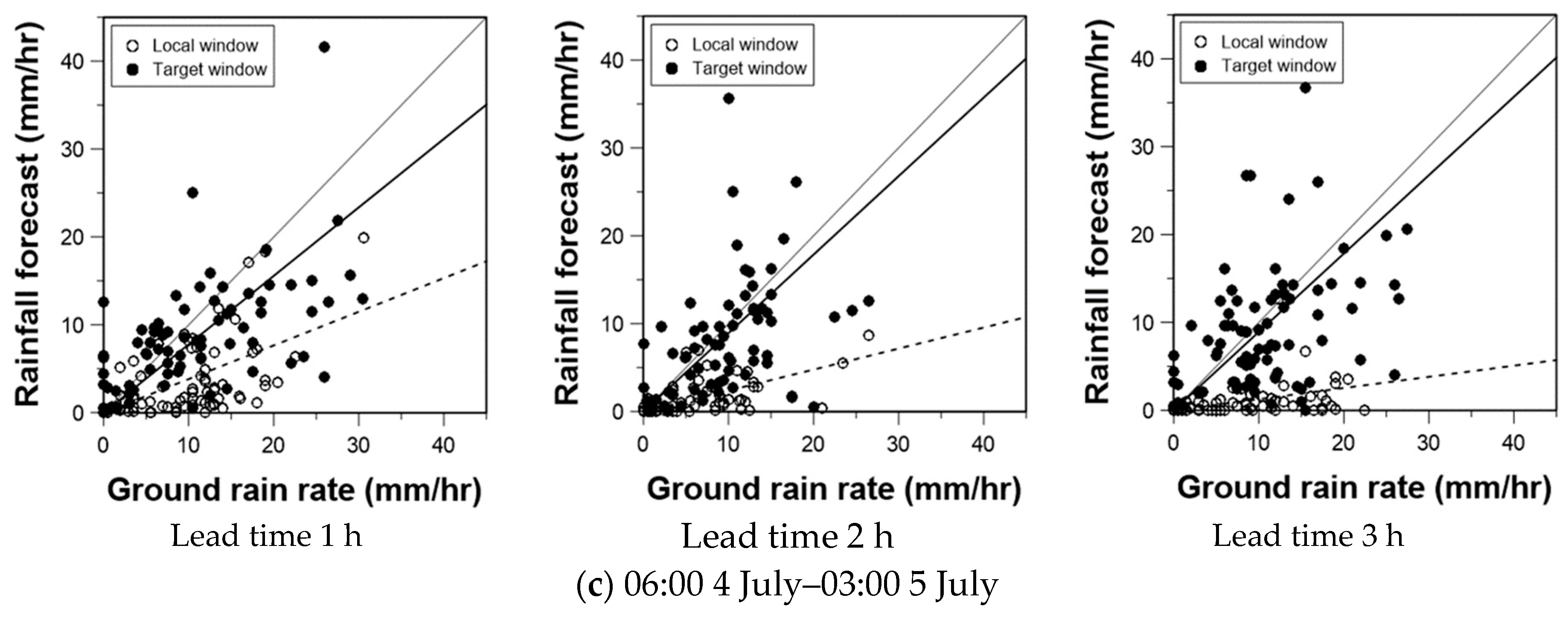
The comparison between the forecasted and the observed data was also done every hour. Figure 7 shows how the comparison result was obtained one-by-one for the storm event that occurred on 4 July. At the beginning of the storm, only one warning site was available with a rain rate higher than 10 mm/h (Figure 7a). After three hours, three warning sites satisfied the minimum condition of rain rate for the backward tracking, meaning that we could get more points for the comparison (Figure 7b). Finally, Figure 7c shows all the comparison results obtained for the entire storm duration.
Several important results can be derived from Figure 7. First, the difference between the conventional method and the proposed method is highly significant. As reviewed in the previous section, the proposed method produced more reasonable results. Even when the number of points was small, the derived slopes were estimated quite reasonably near the one-to-one line. The difference among the three cases of lead times was not found to be significant. That is, the performance of backward tracking was found to be similar regardless of the lead time, at least for these cases of one, two, and three hours. This result is somewhat comparable to that of the conventional method, where the performance became even worse as the lead time increased.
Table 3 also confirmed the same results. The table summarizes the bias correction ratios of all four storm events with their means and standard deviations. Overall, the bias correction ratios estimated by the conventional method were too extreme. Even though in some cases the conventional method also provided reasonable values, it was assumed to be too rare. Also, the bias correction ratio estimated by the conventional method showed a tendency to become worse as the lead time increases, which could not be found in the proposed method based on backward tracking.
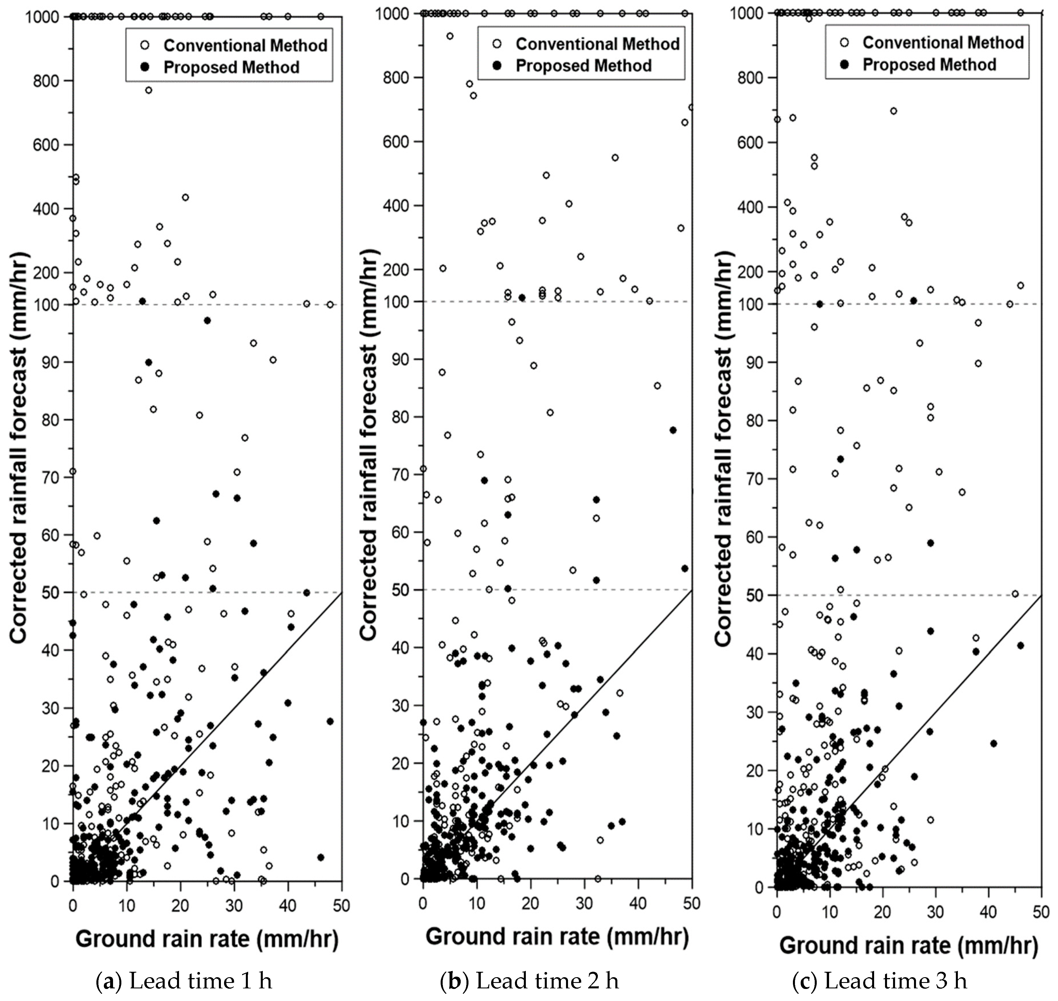
Finally, Figure 8 compares the observed rain rate and the corrected rainfall forecasts by applying the conventional method and the proposed method every hour for every warning site. This comparison was done with all four storm events, and also repeated for the three different lead times. As can be seen in this figure, the corrected rainfall forecasts by applying the proposed method are superior to those made by applying the conventional method. This result is the same for all three cases with different lead times. In all cases, the difference was so huge that it could be easily concluded that the bias correction ratio estimated around the given warning site when there was not enough rain should not be used for the correction of the forecasted rainfall. In some extreme cases, the bias correction ratio was estimated unrealistically to be near zero or infinite. This was because it was possible to have no rain at all (or heavy rain) at the present time, even though there was a heavy (or no) rainfall forecast at the warning site.
5. Conclusions
A flash flood warning system requires the use of rainfall forecasts over the warning site. However, as the rainfall forecast may not satisfy the required quality to be used as input for the warning system, it should be corrected as necessary using the rain gauge information. Unfortunately, the comparison between the observed rainfall data and the rainfall forecasts to correct the bias could not be done properly, as the storm of interest had not arrived at the warning site.
As a detour to overcome this problem, this study proposed a method to estimate the bias correction ratio where the storm was, not at the warning site. This method requires a backward tracking to locate where the forecasted storm at the warning site is at the present time. As the bias correction ratio is estimated where the storm was, it is expected to be more realistic and accurate to correct the bias of rainfall forecast. The proposed method was applied to the MAPLE rainfall forecasts provided by the Korea Meteorological Administration (KMA). A total of 300 warning sites considered in the flash flood warning system for mountain regions in Korea (FFWS-MR) were considered as study sites, along with four different storm events in 2016. The results can be summarized as follows.
First, in most cases of backward tracking, the highest pattern correlation was estimated to be around 0.6. The pattern correlation was, on average, higher for the lead time of one hour, and smaller for the lead time of three hours. However, in all cases, the standard deviations of the pattern correlation were estimated similarly to be about 0.1.
Second, when estimating the bias correction ratio, the difference between the conventional method and the proposed method was highly significant. It was also confirmed that the proposed method provided more reasonable results, even when the number of rain gauges was small. However, the effect of the lead time on the bias correction ratio was not found to be significant. This result was somewhat different from that of the conventional method, where, as the lead time increased, the performance became even worse.
Third, the comparison between the observed rain rate and the corrected rainfall forecasts by applying the conventional method and the proposed method showed that the proposed method was superior to the conventional method. This result was the same for all three cases with different lead times. In all cases, the difference was so huge that it could easily be concluded that the bias correction ratio estimated around the given warning site when the rain rate is low should not be used for the correction of the forecasted rainfall.
The above results show that the proposed method performed much better than the conventional method. In fact, these results can be imagined from the situation that there is no rain at all at the present time at the warning site, even though there is a heavy rainfall forecast. However, it is true that there still remain some limitations to overcome. For example, the size of the window should be determined empirically depending on the storm characteristics. Also, the proposed method cannot be applied if the target window is located over the sea.
Author Contributions
C.Y. conceived and designed the idea of this research and wrote the manuscript. W.N. collected the rainfall forecasts and rain gauge data, and conducted the backward storm tracking to correct the bias.
Funding
This work was supported by the Korea Agency for Infrastructure Technology Advancement (KAIA) grant funded by the Ministry of Land, Infrastructure and Transport (Grant 18AWMP-B127555-02).
Conflicts of Interest
The authors declare no conflict of interest.
References
- Sweeney, T.L. Modernized Areal Flash Flood Guidance; NOAA: Silver Spring, MD, USA, 1992.
- Georgakakos, K.P. On the design of national, real-time warning systems with capability for site-specific, flash-flood forecasts. Bull. Am. Meteorol. Soc. 1986, 67, 1233–1239. [Google Scholar] [CrossRef]
- Ahn, W. A study on the estimation of flash flood index. J. Industitute Ind. Technol. 2000, 15, 11–19. [Google Scholar]
- Bae, D.; Kim, J. Development of Korea flash flood guidance system: (I) Theory and system design. J. Korean Soc. Civ. Eng. 2007, 27, 237–243. [Google Scholar]
- Yoo, C.; Yoon, J.; Ha, E. Sampling error of areal average rainfall due to radar partial coverage. Stoch. Environ. Res. Risk Assess. 2010, 24, 1097–1111. [Google Scholar] [CrossRef]
- Sweeney, T.L.; Fread, D.L.; Georgakakos, K.P. GIS Application for NWS Flash Flood Guidance Model; USGS, WRI: Springfiled, VA, USA, 1993.
- Carpenter, T.M.; Sperfslage, J.A.; Georgakakos, K.P.; Sweeney, T.; Fread, D.L. National threshold runoff estimation utilizing GIS in support of operational flash flood warning systems. J. Hydrol. 1999, 224, 21–44. [Google Scholar] [CrossRef]
- Bhaskar, N.R.; French, M.N.; Kyiamah, G.K. Characterization of Flash Floods in Eastern Kentucky. J. Hydrol. Eng. 2000, 5, 327–331. [Google Scholar] [CrossRef]
- Mukhopadhyay, B.; Cornelius, J.; Zehner, W. Application of kinematic wave theory for predicting flash flood hazards on coupled alluvial fan-piedmont plain landforms. Hydrol. Process. 2003, 17, 839–868. [Google Scholar] [CrossRef]
- Ogden, F.L.; Sharif, H.O.; Senarath, S.U.S.; Smith, J.A.; Baeck, M.L.; Richardson, J.R. Hydrologic analysis of the Fort Collins, Colorado, flash flood of 1997. J. Hydrol. 2000, 228, 82–100. [Google Scholar] [CrossRef]
- Borga, M.; Boscolo, P.; Zanon, F.; Sangati, M. Hydrometeorological analysis of the 29 August 2003 flash flood in the Eastern Italian Alps. J. Hydrometeorol. 2007, 8, 1049–1067. [Google Scholar] [CrossRef]
- Nikolopoulos, E.I.; Anagnostou, E.N.; Borga, M.; Vivoni, E.R.; Papadopoulos, A. Sensitivity of a mountain basin flash flood to initial wetness condition and rainfall variability. J. Hydrol. 2011, 402, 165–178. [Google Scholar] [CrossRef]
- Ruiz-Villanueva, V.; Diez-Herrero, A.; Stoffel, M.; Bollschweiler, M.; Bodoque, J.M.; Ballesteros, J.A. Dendrogeomorphic analysis of flash floods in a small ungauged mountain catchment (Central Spain). Geomorphology 2010, 118, 383–392. [Google Scholar] [CrossRef]
- Shin, H.; Kim, H.; Park, M. The study of the fitness on calculation of the flood warning trigger rainfall using GIS and GCUH. J. Korea Water Resour. Assoc. 2004, 37, 407–424. [Google Scholar] [CrossRef]
- Mueller, C.; Saxen, T.; Roberts, R.; Wilson, J.; Betancourt, T.; Dettling, S.; Oien, N.; Yee, J. NCAR Auto-Nowcast System. Weather Forecast 2003, 18, 545–561. [Google Scholar] [CrossRef]
- Dixon, M.; Wiener, G. Titan—Thunderstorm Identification, Tracking, Analysis, and Nowcasting—A Radar-Based Methodology. J. Atmos. Ocean Technol. 1993, 10, 785–797. [Google Scholar] [CrossRef]
- Saito, K.; Fujita, T.; Yamada, Y.; Ishida, J.I.; Kumagai, Y.; Aranami, K.; Ohmori, S.; Nagasawa, R.; Kumagai, S.; Muroi, C.; et al. The operational JMA nonhydrostatic mesoscale model. Mon. Weather Rev. 2006, 134, 1266–1298. [Google Scholar] [CrossRef]
- Teradar, M. The development of short-term rainfall prediction system in mountainous region by the combination of extrapolation model and meso-scale atmospheric model. In Proceedings of the 6th International Symposium on Hydrolojical Applications of Weather Radar, Melbourne, Australia, 2–4 February 2004. [Google Scholar]
- Bellon, A.; Austin, G.L. Evaluation of 2 Years of Real-Time Operation of a Short-Term Precipitation Forecasting Procedure (Sharp). J. Appl. Meteorol. 1978, 17, 1778–1787. [Google Scholar] [CrossRef]
- Germann, U.; Zawadzki, I. Scale-dependence of the predictability of precipitation from continental radar images. Part I: Description of the methodology. Mon. Weather Rev. 2002, 130, 2859–2873. [Google Scholar] [CrossRef]
- Germann, U.; Zawadzki, I.; Turner, B. Predictability of precipitation from continental radar images. Part IV: Limits to prediction. J. Atmos. Sci. 2006, 63, 2092–2108. [Google Scholar] [CrossRef]
- Radhakrishna, B.; Zawadzki, I.; Fabry, F. Predictability of Precipitation from Continental Radar Images. Part V: Growth and Decay. J. Atmos. Sci. 2012, 69, 3336–3349. [Google Scholar] [CrossRef]
- Turner, B.J.; Zawadzki, I.; Germann, U. Predictability of precipitation from continental radar images. Part III: Operational nowcasting implementation (MAPLE). J. Appl. Meteorol. 2004, 43, 231–248. [Google Scholar] [CrossRef]
- Korea Meteorological Administration (KMA). Study on the Weather Radar Application (II); KMA: Seoul, Korea, 2008.
- Atencia, A.; Zawadzki, I.; Berenguer, M. Scale Characterization and Correction of Diurnal Cycle Errors in MAPLE. J. Appl. Meteorol. Clim. 2017, 56, 2561–2575. [Google Scholar] [CrossRef]
- Munoz, C.; Wang, L.P.; Willems, P. Enhanced object-based tracking algorithm for convective rain storms and cells. Atmos. Res. 2018, 201, 144–158. [Google Scholar] [CrossRef]
- Novo, S.; Martinez, D.; Puentes, O. Tracking, analysis and nowcasting of Cuban convective cells as seen by radar. Meteorol. Appl. 2014, 21, 585–595. [Google Scholar] [CrossRef]
- Yang, L.; Smith, J.A.; Baeck, M.L.; Bou-Zeid, E.; Jessup, S.M.; Tian, F.Q.; Hu, H.P. Impact of Urbanization on Heavy Convective Precipitation under Strong Large-Scale Forcing: A Case Study over the Milwaukee-Lake Michigan Region. J. Hydrometeorol. 2014, 15, 261–278. [Google Scholar] [CrossRef]
- Shah, S.; Notarpietro, R.; Branca, M. Storm Identification, Tracking and Forecasting Using High-Resolution Images of Short-Range X-Band Radar. Atmosphere 2015, 6, 579–606. [Google Scholar] [CrossRef] [Green Version]
- Hubbert, J.C.; Dixon, M.; Ellis, S.M. Weather Radar Ground Clutter. Part II: Real-Time Identification and Filtering. J. Atmos. Ocean Technol. 2009, 26, 1181–1197. [Google Scholar] [CrossRef]
- Hubbert, J.C.; Dixon, M.; Ellis, S.M.; Meymaris, G. Weather Radar Ground Clutter. Part I: Identification, Modeling, and Simulation. J. Atmos. Ocean Technol. 2009, 26, 1165–1180. [Google Scholar] [CrossRef]
- Islam, T.; Rico-Ramirez, M.A.; Han, D.W.; Srivastava, P.K. Artificial intelligence techniques for clutter identification with polarimetric radar signatures. Atmos. Res. 2012, 109, 95–113. [Google Scholar] [CrossRef]
- Yoo, C.; Yoon, J. The error structure of the CAPPI and the correction of the range dependent error due to the earth curvature. Atmosphere 2012, 22, 309–319. [Google Scholar] [CrossRef]
- Austin, P.M. Relation between Measured Radar Reflectivity and Surface Rainfall. Mon. Weather Rev. 1987, 115, 1053–1071. [Google Scholar] [CrossRef]
- Collier, C.G. Accuracy of Rainfall Estimates by Radar. 1. Calibration by Telemetering Rain-Gages. J. Hydrol. 1986, 83, 207–223. [Google Scholar] [CrossRef]
- National Disaster Management Research Institute (NDMI). Advancement of Mountain Flash Flood Prediction System & Development of Decision-Making Supporting System; NDMI: Seoul, Korea, 2010.
- Germann, U.; Zawadzki, I. Scale dependence of the predictability of precipitation from continental radar images. Part II: Probability forecasts. J. Appl. Meteorol. 2004, 43, 74–89. [Google Scholar] [CrossRef]
- Huff, F.A. Time Distribution of Rainfall in Heavy Storms. Water Resour. Res. 1967, 3, 1007–1019. [Google Scholar] [CrossRef]
- Clayton, A.J.; Deacon, R.C. The Investigation of Local Patterns of Precipitation and Storm Movement Using Computer Techniques; Department of Civil Engineering, Bristol University: Bristol, UK, 1971. [Google Scholar]
- Marshall, R.J. The Estimation and Distribution of Storm Movement and Storm Structure, Using a Correlation-Analysis Technique and Rain-Gauge Data. J. Hydrol. 1980, 48, 19–39. [Google Scholar] [CrossRef]
- Niemczynowicz, J. Storm Tracking Using Rain-Gauge Data. J. Hydrol. 1987, 93, 135–152. [Google Scholar] [CrossRef]
- Wilson, J.W. Integration of radar and raingage data for improved rainfall measurement. J. Appl. Meteorol. 1970, 9, 489–497. [Google Scholar] [CrossRef]
- Leese, J.A.; Charles, S.N.; Bruce, B.C. An automated technique for obtaining cloud motion from geosynchronous satellite data using cross correlation. J. Appl. Meteorol. 1971, 10, 118–132. [Google Scholar] [CrossRef]
- Austin, G.L.; Bellon, A. The use of digital weather radar records for short-term precipitation forecasting. Q. J. R. Meteorol. Soc. 1974, 100, 658–664. [Google Scholar] [CrossRef]
- Rinehart, R.E.; Garvey, E.T. 3-Dimensional Storm Motion Detection by Conventional Weather Radar. Nature 1978, 273, 287–289. [Google Scholar] [CrossRef]
- Hilst, G.R.; Russo, J.A. An Objective Extrapolation Technique for Semi-Conservative Fields with an Application to Radar Patterns; Travelers Insurance Companies: Hartford, CT, USA, 1960. [Google Scholar]
- Kim, G.; Kim, J.P. Development of a short-term rainfall forecasting model using weather radar data. J. Korea Water Resour. Assoc. 2008, 41, 1023–1034. [Google Scholar] [CrossRef]
- Brandes, E.A. Optimizing Rainfall Estimates with Aid of Radar. J. Appl. Meteorol. 1975, 14, 1339–1345. [Google Scholar] [CrossRef]
- Lin, D.S. An Application of Recursive Methods to Radar-Rainfall Estimation. Master’s Thesis, University of Iowa, Iowa City, IA, USA, 1989. [Google Scholar]
- Anagnostou, E.N.; Krajewski, W.F. Real-time radar rainfall estimation. Part I: Algorithm formulation. J. Atmos. Ocean Technol. 1999, 16, 189–197. [Google Scholar] [CrossRef]
- Anagnostou, E.N.; Krajewski, W.F.; Seo, D.J.; Johnson, E.R. Mean-Field Rainfall Bias Studies for Wsr-88d. J. Hydrol. Eng. 1998, 3, 149–159. [Google Scholar] [CrossRef]
- Yoo, C.; Kim, J.; Jung, J.; Yang, D. Mean field bias correction of the very-short-range-forecast rainfall using the kalman filter. J. Korean Soc. Hazard Mitig. 2011, 11, 17–28. [Google Scholar] [CrossRef]
- Lee, J.; Yoon, J.; Jeon, H. Evaluation for the correction of radar rainfall due to the spatial distribution of raingauge network. J. Korean Soc. Hazard Mitig. 2014, 14, 337–345. [Google Scholar] [CrossRef]
- Yoo, C.; Park, C.; Yoon, J. Decision or G/R ratio for the correction of mean-field bias of radar rainfall and linear regression problem. J. Korean Soc. Civ. Eng. 2011, 31, 393–403. [Google Scholar]
Figure 1.
Storm tracking within the search domain (circle) based on the pattern correlation between local window (a) and target window (b) (the number inside the cell represents rainfall intensity).
Figure 1.
Storm tracking within the search domain (circle) based on the pattern correlation between local window (a) and target window (b) (the number inside the cell represents rainfall intensity).

Figure 2.
Comparison of the conventional method (a) and the proposed method in this study (b) for estimating the bias correction ratio.
Figure 2.
Comparison of the conventional method (a) and the proposed method in this study (b) for estimating the bias correction ratio.

Figure 3.
A total of 300 flash flood warning sites over the Korean Peninsula and the location of the Ducsanggi Valley (inside the solid box) considered as an example in this study.
Figure 3.
A total of 300 flash flood warning sites over the Korean Peninsula and the location of the Ducsanggi Valley (inside the solid box) considered as an example in this study.

Figure 4.
Radar images of four storm events considered in this study.

Figure 5.
Local window (black solid box in (a)) made for the Ducsanggi Valley over the two-hour rainfall forecasts made at 18:00 4 July 2016 and the resulting target window (blue solid box in (b)) determined by applying the backward tracking method over the two-hour rainfall forecasts made at 16:00 at the same day.

Figure 6.
Comparison results of ground data and rainfall forecast at the local and target windows for the Ducsanggi Valley as an example (16:00 4 July).
Figure 6.
Comparison results of ground data and rainfall forecast at the local and target windows for the Ducsanggi Valley as an example (16:00 4 July).

Figure 7.
Comparison results of ground data and rainfall forecast at the local and target windows for the rainfall event on 4 July (a) at the beginning of rainfall, (b) after three hours, and (c) all the available cases.
Figure 7.
Comparison results of ground data and rainfall forecast at the local and target windows for the rainfall event on 4 July (a) at the beginning of rainfall, (b) after three hours, and (c) all the available cases.


Figure 8.
Comparison of corrected rainfall forecasts in the local window with the ground rainfall data (a) for the lead time of 1 h, (b) for the lead time of 2 h, and (c) for the lead time of 3 h.
Figure 8.
Comparison of corrected rainfall forecasts in the local window with the ground rainfall data (a) for the lead time of 1 h, (b) for the lead time of 2 h, and (c) for the lead time of 3 h.


Table 1.
Basic characteristics of four storm events that occurred in 2016.
| Event | Duration (h) | Maximum Rainfall Intensity (mm/h) | Most Severely Affected Area | Moving Direction |
|---|---|---|---|---|
| 1 | 04:00 4 July–03:00 5 July (24) | 34.5 | Central |  (NE) (NE) |
| 2 | 05:00 5 July–03:00 6 July (23) | 57.1 | Eastern |  (SE) (SE) |
| 3 | 21:00 2 October–15:00 3 October (20) | 18.3 | Northern | (SE) |
| 4 | 23:00 4 October–14:00 5 October (17) | 98.3 | Southern | (NE) |
Table 2.
Means and standard deviations (within the parenthesis) of pattern correlation estimated for four storm events that occurred in 2016.
Table 2.
Means and standard deviations (within the parenthesis) of pattern correlation estimated for four storm events that occurred in 2016.
| Storm Event | Lead Time | ||
|---|---|---|---|
| 1 h | 2 h | 3 h | |
| 4–5 July | 0.630 (0.116) | 0.656 (0.075) | 0.601 (0.054) |
| 5–6 July | 0.617 (0.095) | 0.645 (0.101) | 0.558 (0.051) |
| 2–3 October | 0.678 (0.075) | 0.623 (0.102) | 0.594 (0.129) |
| 4–5 October | 0.600 (0.128) | 0.524 (0.132) | 0.566 (0.133) |
| Average | 0.633 (0.107) | 0.620 (0.112) | 0.584 (0.103) |
Table 3.
Means and standard deviations (within the parenthesis) of bias correction ratio estimated for each storm event with respect to the lead time.
Table 3.
Means and standard deviations (within the parenthesis) of bias correction ratio estimated for each storm event with respect to the lead time.
| Storm Event | Lead Time | |||||
|---|---|---|---|---|---|---|
| 1 h | 2 h | 3 h | ||||
| Conventional | Proposed | Conventional | Proposed | Conventional | Proposed | |
| 4–5 July | 7.937 (22.381) | 1.736 (1.402) | 11.853 (16.678) | 1.227 (0.983) | 11.420 (25.323) | 1.145 (1.674) |
| 5–6 July | 12.385 (22.163) | 1.716 (1.200) | 21.362 (27.607) | 2.059 (1.589) | 23.392 (37.820) | 0.791 (0.471) |
| 2–3 October | 2.081 (5.008) | 0.955 (1.341) | 1.197 (3.513) | 0.476 (0.452) | 1.665 (2.565) | 0.239 (0.212) |
| 4–5 October | 2.277 (2.585) | 1.069 (0.683) | 5.612 (5.557) | 1.295 (1.250) | 5.447 (6.496) | 0.894 (0.637) |
| All | 6.798 (17.628) | 1.450 (1.285) | 8.786 (15.506) | 1.265 (1.228) | 8.453 (20.859) | 0.812 (1.154) |
© 2018 by the authors. Licensee MDPI, Basel, Switzerland. This article is an open access article distributed under the terms and conditions of the Creative Commons Attribution (CC BY) license (http://creativecommons.org/licenses/by/4.0/).
Share and Cite
MDPI and ACS Style
Na, W.; Yoo, C. A Bias Correction Method for Rainfall Forecasts Using Backward Storm Tracking. Water 2018, 10, 1728. https://doi.org/10.3390/w10121728
AMA Style
Na W, Yoo C. A Bias Correction Method for Rainfall Forecasts Using Backward Storm Tracking. Water. 2018; 10(12):1728. https://doi.org/10.3390/w10121728
Chicago/Turabian StyleNa, Wooyoung, and Chulsang Yoo. 2018. "A Bias Correction Method for Rainfall Forecasts Using Backward Storm Tracking" Water 10, no. 12: 1728. https://doi.org/10.3390/w10121728
Note that from the first issue of 2016, this journal uses article numbers instead of page numbers. See further details here.