An Improvement of Port-Hamiltonian Model of Fluid Sloshing Coupled by Structure Motion

1
Department for Management of Science and Technology Development, Ton Duc Thang University, Ho Chi Minh City 700000, Vietnam
2
Faculty of Civil Engineering, Ton Duc Thang University, Ho Chi Minh City 700000, Vietnam
Water 2018, 10(12), 1721; https://doi.org/10.3390/w10121721
Submission received: 2 November 2018
/
Revised: 16 November 2018
/
Accepted: 21 November 2018
/
Published: 24 November 2018
(This article belongs to the Special Issue Pipeline Fluid Mechanics)
Abstract
:The fluid–solid interaction is an interesting topic in numerous engineering applications. In this paper, the fluid–solid interaction is considered in a vessel attached to the free tip of a cantilever beam. Governing coupled equations of the system include the Euler–Bernoulli equation for bending of a beam, torsion of a beam, 2-D motion of the rigid vessel, and rotating shallow water equation of fluid sloshing in the vessel. As an essential portion in the numerical simulation of the vibration control of this fluid–plate system is the accurate modeling of sloshing; the partial differential equations of the system are modified by approximation of velocity profile. The suggested method is validated by experimental results of a piezoelectric actuated clamped rectangular plate holding a cylindrical vessel. These sloshing interactions with elastic test cases illustrate the mass conservative characteristics of the method as well as its stability in a prompt change of the vessel situations.
1. Introduction
The problem of simulating the interaction between fluids (water and air) and structure (tank wall) in partially filled storage vessels is discussed in many kinds of research as it is of interest to numerous industrial applications, for instance, marine science, aircraft design, seismic engineering, and fuel vessels in vehicles. In the study of fluid–structure interaction (FSI) in sloshing tanks, the numerical investigation is reasonably efficient and cheaper than the full-scale experiments [1]. Nicolici and Bilegan [2] studied the earthquake excited sloshing in flexible tanks by one-way coupling of finite element method (FEM) and computational fluid dynamics (CFD) techniques. They found that the wall elasticity augments the impulsive pressure.
As the excitation frequency of the system approaches the sloshing fundamental frequency, it can hurt the other structures in the system. Since the study of sloshing is more important in this field [3], time-independent smoothed particle hydrodynamics [4] and finite difference analysis [5] of viscous and inviscid fluid sloshing in a rectangular domain is performed by researchers. The impact of sloshing water on walls [3,6,7] is not negligible and can affect the coupled system response. The smoothed-particle hydrodynamics (SPH) computational method is a mesh-free Lagrangian method which considers the fluid as the collection of separate particles [8]. These particles affect each other over a smoothing length with a kernel function (such as cubic spline and Gaussian) [9].
The advantages of SPH over traditional grid-based methods are higher accuracy, guaranteed mass conservation, higher performance in large distortion conditions, pressure evaluation by neighboring particles, and easy free surface tracking [10]. On the other hand, the disadvantages of SPH are in the evaluation of free surface by polygonization method, lower performance in small distortion conditions, and numerous particles requirements [11,12]. Although the SPH method is used for solid mechanics computations [13,14,15], due to its instability in tensile case (stretching cause the tear) [15], first-type boundary conditions (Dirichlet) [16], and high computational cost [17], the solid part in this paper is done by finite element method. The common method in the literature for solid–liquid interaction problems is the use of SPH for the fluid part and FE for solid part [17,18,19,20]. In the works of Johnson [17,18] and Attaway [19], the SPH–FEM interface is controlled by FE motion while at each FE point the force is calculated from the nearest SPH particles. Since this method cannot be considered a conservative interface method, to have an interface preserving method with a higher computational cost method, Sonia Fernández-Méndez et al. [20] defined a buffer zone in FSI interface that is affected by both zones but does not allow the SPH and FEM to interrupt each other. Recently, the study of sloshing–plate interaction is performed in various studies [21,22,23]. In the study of Yu et al. [21], the plate is located within the sloshing system, while, in the studies of Kotyczka and Maschke [22] and Ribeiro et al. [23], the solid system is confined the sloshing. Ribeiro et al. proposed the FEM-based port-Hamiltonian formulation with the Saint-Venant approximation for Shallow Water Equations (SWE). Their port-Hamiltonian model of liquid sloshing in moving containers is applied to a fluid–structure system [23]. To control the liquid sloshing dynamics [24], Lasiecka and Tuffaha [25] used the boundary feedback control in fluid–structure interactions. This method is the solution to some automatic control problems for sloshing phenomena and water–tank systems [26,27]. Coron [28] investigated the local controllability of a 1-D tank containing a fluid modeled by applying the calculus of variations on the shallow water equations. In addition, the stabilization problem of a 1-D tank containing a fluid modeled by the shallow water equations was solved by Prieur and Halleux [29]. This method was used by Robu [30] to active vibration control of a fluid–plate system.
As it is important in the port-Hamiltonian systems theory, the modeling of each part plays a significant role in the numerical calculation of the whole system [31]. In the various research for a coupled fluid–plate system excited by piezoelectric actuators, the authors use the linearized shallow water equation for the fluid part in the water–tank system [30,32,33,34]. Such simple models are also used for the control problems for water–tank systems [26], dynamic coupling between shallow-water sloshing and horizontal vehicle motion [35], sloshing in vessels undergoing prescribed rigid-body motion in three dimensions [36], and stabilization of a one-dimensional tank containing a fluid modeled by the shallow water equations [29]. The shallow water equation is also recently studied in the port-Hamiltonian framework but with a different goal: modeling and controlling the flow on open channel irrigation systems [37,38]. In this case, there is neither rotation nor translation of the channels. The effect of the nonlinear term has not been considered in the literature.
The aim of the current manuscript is to present a new dynamic simulating of the coupled system by driving the equation of motion from the port-Hamilton method and consider the nonlinear effects of fluid on the system by a comprehensive model. By the new modifications, the accuracy of the port-Hamiltonian formalism is improved. First, the state equation of the moving container system is derived and benchmarked by the frequency response of the coupled system. Second, the code is validated by experimental results and shows the improvement of the prediction of liquid sloshing response. New improvements offer a better model of sloshing which augment the accuracy of simulation in association with arbitrarily complex vibrational systems. Finally, the importance of each mode of energy is discussed in the coupled system.
2. Mathematical Modeling
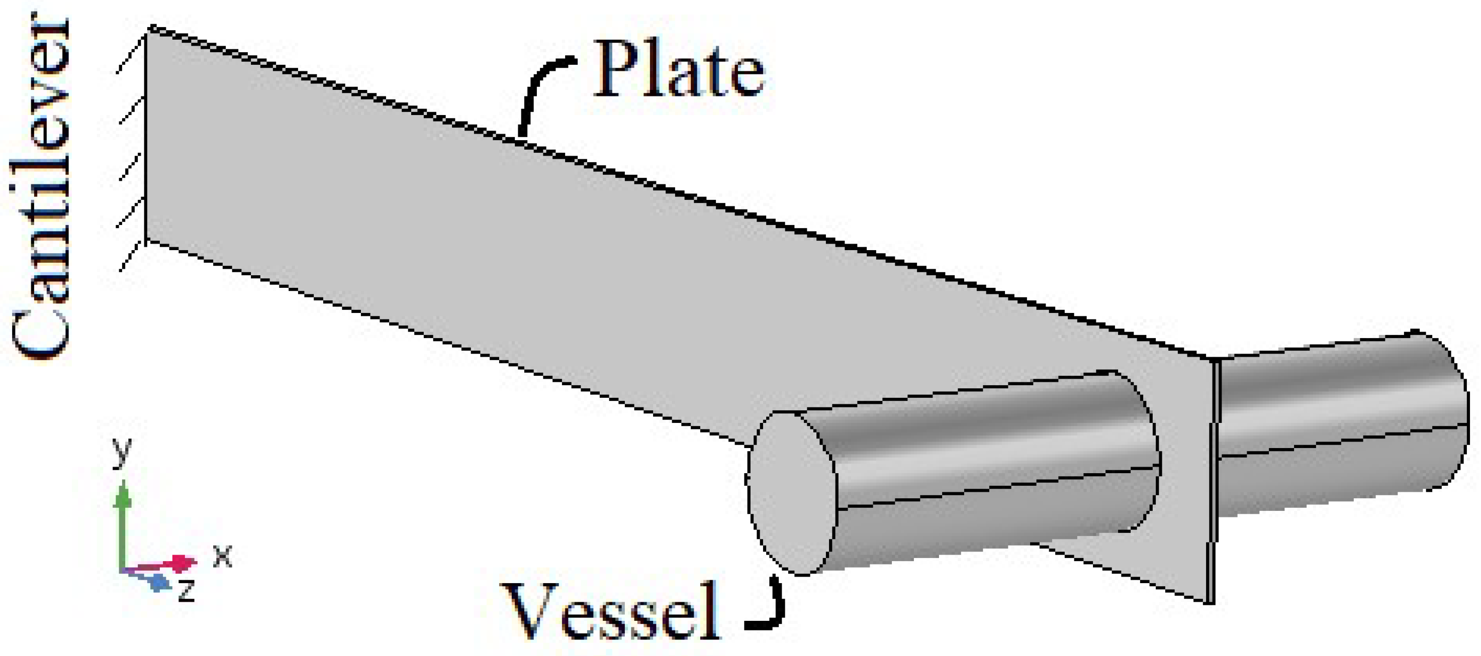
The fluid, structure and rigid body considered in the current problem are plotted in Figure 1. The system shown in Figure 1 includes a cantilevered aluminum plate with a plastic vessel mounted by fixation rings near the free end. The actuator/sensor patches are used to control the vibration of the moving container system. Table 1 presents the geometrical parameters and physical properties of the system. Here, the solid plate is assumed as a bending and torsion element with Euler–Bernoulli beam model where the bending and torsional modes are operating individually. Subsystems are considered to affect each other by kinetic and kinematic interactions. The experimental system from Ribeiro et al. [23] was chosen to compare the numerical simulation with experimental results. Their experimental rig is designed for the application of airplane fuel tank and wing design where the light materials adopted for the wing caused low fundamental frequency as the order of sloshing frequency. Navier–Stokes fluid flow is modeled through the following mass and momentum conservation equations:
where u, , and g are vectors and presented in bold. The equation inside the boundary layer is in x-direction
and for y-direction
Outside the bottom boundary layer, the potential flow is dominated
with the zero velocities on the walls
constant pressure at the free surface
And kinematic velocity at the free surface
The Cartesian components of acceleration of the rotating system are:
By the use of velocity potential:
and integration of continuity equation versus y
which leads to
To derive a linearized form of momentum equation, first the pressure term should be evaluated. By y integration of the momentum equation in y-direction
and differentiate with respect to x
the first term in Equation (13) is simplified by the aid of Leibniz rule
where the use of velocity potential the second term in the above equation is simplified as
In addition, the second term in Equation (18) is simplified by the aid of Leibniz rule
Finally, Equations (17)–(21) result in
where the last term in Equation (22) could be rewritten by the use of in the form
inside the boundary layer and outside the bottom boundary layer is
Integrating the above equations from the bottom to free with surface respect to z-direction divided by the total length,
where δ is the length of the boundary layer. Replacing the vertical velocity in inertial term with
causes to the following simplification
and the time variance of vertical velocity in Equation (24) with (inviscid limit )
The viscous term in Equation (21) is simplified by Stokes first problem. The viscous term in Equation (25) is rewritten as
If the bottom wall velocity is and considering the viscous effect and neglecting the inertial effect, the governing boundary layer equation by
If the semi-infinite fluid zone is considered, which has the solution of error function, there is no geometric length scale
If we consider a bounded solution,
the bottom shear is
where . Equation (33) can be simplified to
Finally, Equation (23) is rewritten as
The friction is found with a linear relation of top velocity by the coefficient of
where the shear at the boundary layer is ignored () and the shear at the bottom is replaced by Stokes first problem value (), a factor because of phase difference between velocity and shear, and the factor () because of side effect. The governing equations presented in Equations (15) and (25) with the simplifications of Equations (26)–(36) are summarized in
where , , and .
By Equations (16) and (37), the 1-D equation of motion is completed while the coupling the frequencies are a significant problem in design.
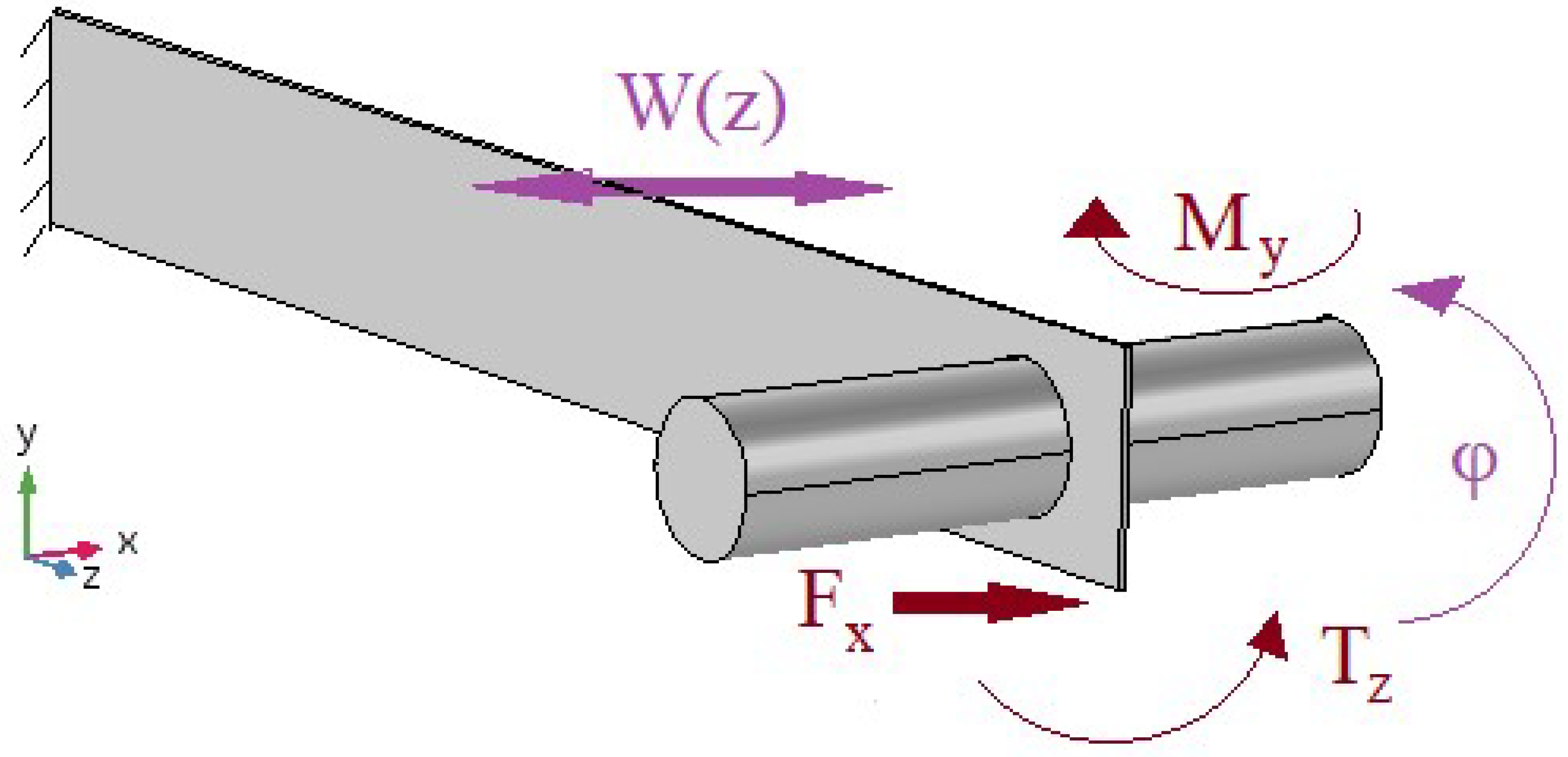
To model the dynamics of the system, it could be considered in two subsystems: a beam with torsion and bending mode of freedom (Figure 2) and a fluid in a moving vessel (Figure 3).
The equations presented here could be derived from the classical Lagrangian method. The Lagrangian of vessel moving by external force and solid connected in base is
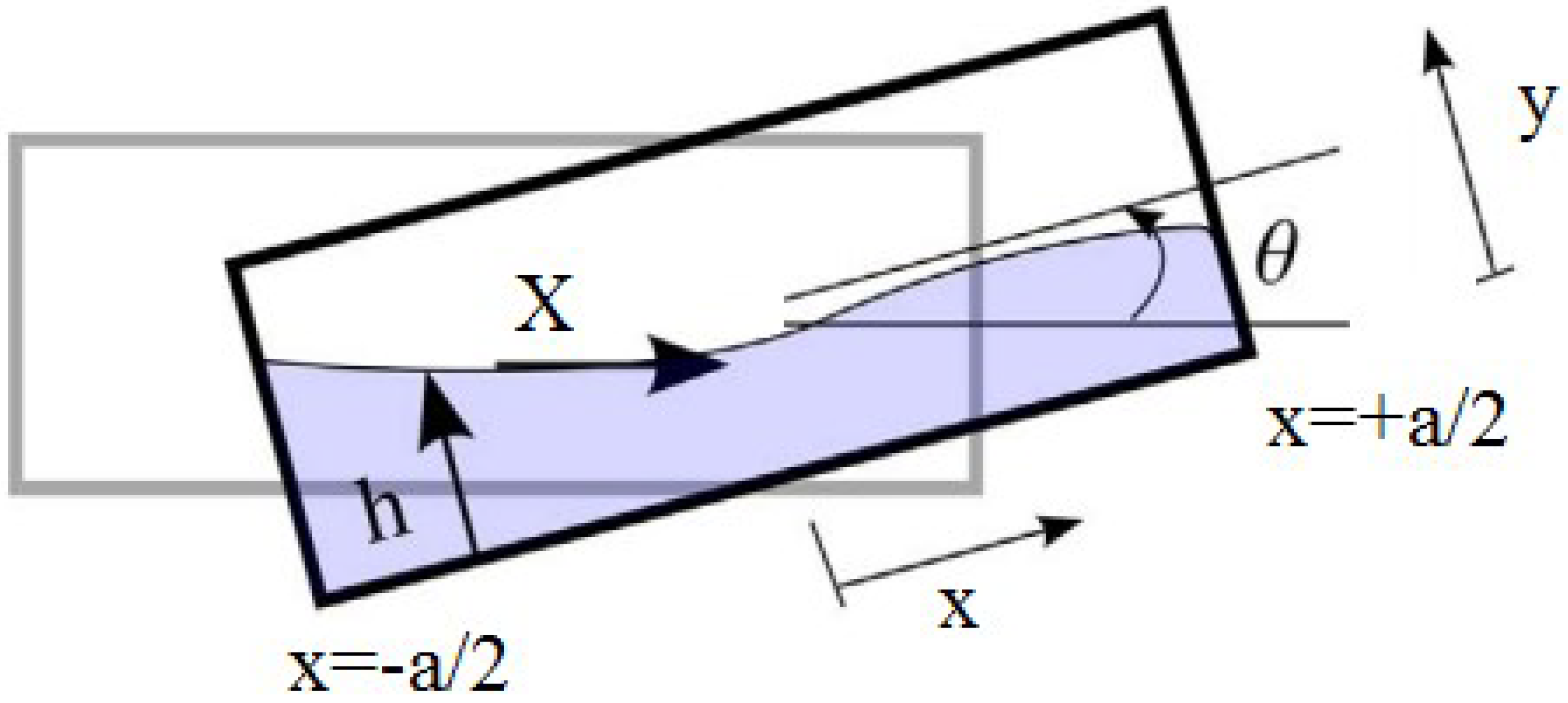
where the system is described by the following quantities: a is the tank length; b is the tank width; ρ is the fluid density; g is the gravity; mv is the mass of the empty vessel; X(t) represents the horizontal position of the vessel (with respect to an inertial frame); x is the position along the vessel (measured in local coordinates from the middle of the vessel); h(x,t) is the height profile of fluid (−a/2 < x < a/2); and u(x,t) is the fluid speed (measured relative to the vessel).
The assumptions are:
- The fluid and the tank are viewed as an open system.
- The fluid governing equations are obtained from Euler–Lagrange formulation.
- There is no flow through the tank walls.
- The effect of rigid-body inertias of the tank and the mass of the tank is considered.
- The structure is considered a beam with two independent bending and torsion motions.
- Because of symmetrical installation of the piezoelectric patches along the torsion axis, their effect on torsional motion is neglected.
- The piezoelectric patches actuation affects only the bending motion of the beam.
- Here, the linear Euler–Bernoulli beam with distributed piezoelectric actuators is used for the bending.
- The electric field is constant through the piezoelectric patch thickness.
- The voltage is uniform along the patch.
- The beam is considered as a long beam under small displacements.
- The fixed end for the torsion and for the bending is considered at the clamped point.
- A weak formulation is used to overwhelm the derivation of the non-smoothness function.
By introducing the constraint of
which is obtained from mass conservation, the following variational problem of finding the minimum Lagrangian (where constraints are adjoined by Lagrange multiplier) is obtained:
To find the governing equations of the system, for any small variation of of h such that , Equation (40) yields
and then, thanks to an integration by parts,
since
In addition, for any small variation of of u such that , and the boundary condition of , Equation (36) yields
and then, thanks to an integration by parts,
Replacing the value of by Equation (45) into Equation (43),
A differentiation with respect to x and use of Equation (45) yields
which is the momentum conservation equation.
where and . As the system is controlled by a piezoelectric sheet, the following function is added to the bending function:
The Hamiltonian of the parts of the system, equation of motion of the parts of the system, and boundary condition of the system are presented in Table 2, Table 3 and Table 4, respectively.
For the node i = 1 to Nb, the discretized bending equations are
For the node i = 1 to Nt, the discretized torsion equations are
For the node i = 1 to Nf, the discretized shallow water equations are
The equations of motion of the rigid body of vessel are linear momentum in x-direction, angular momentum in z-direction, and angular momentum in y-direction:
The total mass of the rigid body contains mass of the empty vessel (me = ρπ·Lout·(Dout2 − Din2)/4), the tip mass (mtip), the mass of two fixation rings (mring = 2ρ ring·π·tring·((Doutring)2 − (Dinring)2)/4), and reduction of plate hole mass (mh = ρbπ·tb·Dout2/4). The tip mass (mtip), located at the vessel tip, consists of plastic disc, glue, and a plug. Although it is not a simple geometry, here, the effects on the system mass and inertia are approximated as a point mass (mR = me + mtip + mring − mh).
The Ir is total vessel mass moment of inertia around the z-direction, since vessel and fixation rings are symmetric around the z-axis. The total vessel mass moment of inertia is the sum of the empty vessel inertia (Ie = me (3/4(Dout2 − Din2) + Lout2)/12), the tip mass inertia (Itip = mtipLtip2), the mass of two fixation rings (Iring = mring/12(3/4 ((Dout ring)2 + (Din ring)2) + (tring)2)), and reduction of plate hole mass (Ih = mh·Dout2/16).
The JR is total mass moment of inertia around the y-direction (JR = Ir + If) Total vessel mass moment of inertia around the y-direction is the sum of vessel moment of inertia around the y-direction, which is similar to Ir·(JR = Ie + Itip + Iring − Ih) and the frozen fluid mass moment of inertia
Finally, the fluid–solid dynamic coupling equations are
If the cylindrical vessel is filled to the height h (0 < h < Din), then the total volume of the fluid is
where the filling angle, α, is found from . The effective depth of the equivalent rectangular vessel is found from the depth of the fluid in the cylindrical vessel at rest
and the effective length of the equivalent rectangular vessel is found from depth and equivalent volume (Leq = Vf/Wv).
3. Numerical Results
Having implemented the FE in a MATLAB-based code, the resulting transient problem is then solved to determine the coupled response of illustrative beam motion, subjected to the various boundary and load conditions. In this section, first, the code is validated by comparison of the frequency response of the coupled system with experimental results of reference [23]; and, second, the state equation of the system is solved and the dynamic of the variables of the system is shown versus time. The most important parameters are the sloshing phenomenon (regarding evolutions of the free surface) in a moving tank and displacement and rotation of the structure and rigid body which is numerically investigated. By varying the time, interesting characteristics, such as sub-system energies, and dynamic responses of the structures in both time and frequency domains are presented.
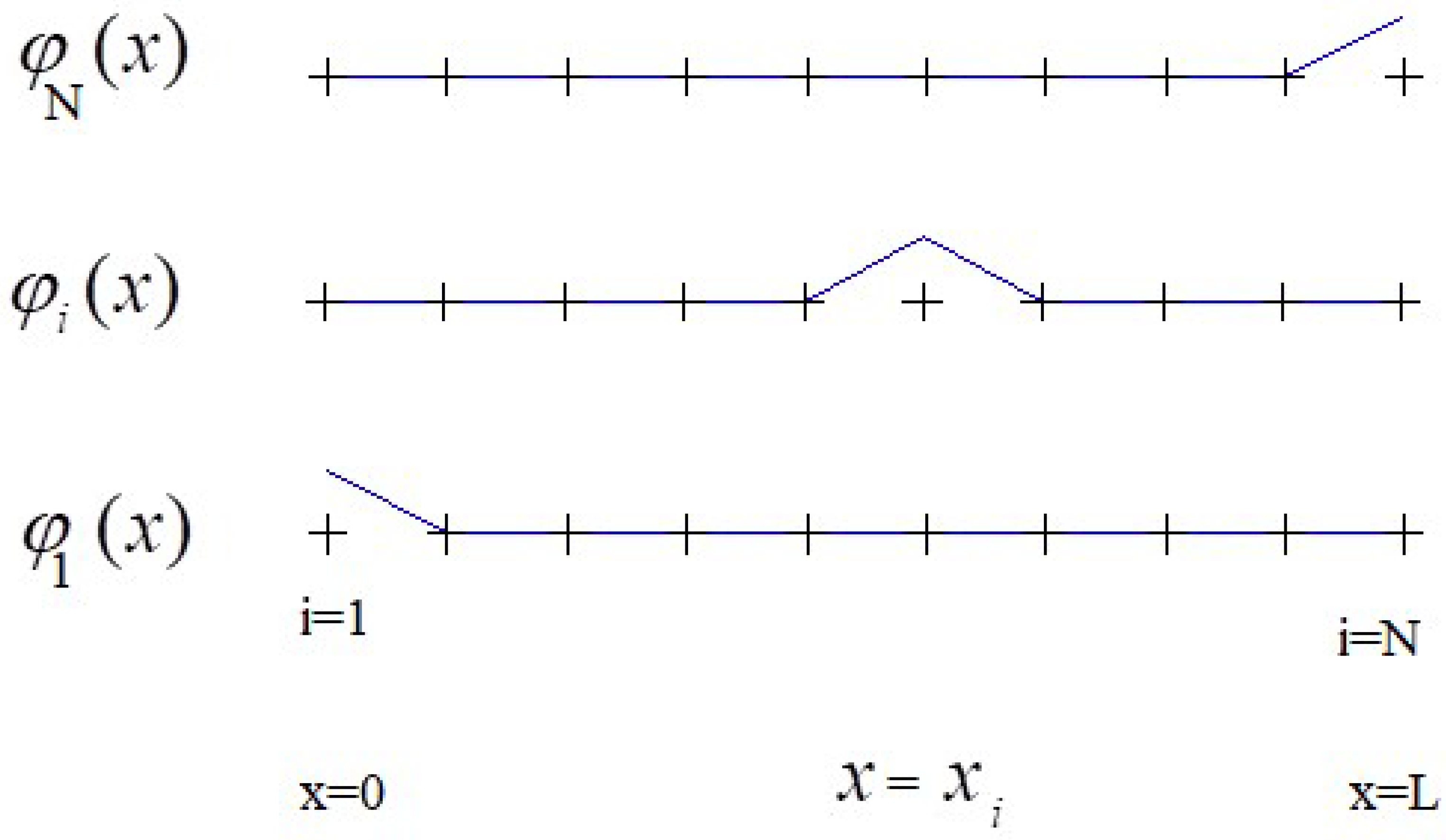
To choose basis functions ϕi for finite element method with the property of being one at the point i and zero at the other points, the simple linear functions are used. As shown in Figure 4, the simplest choice of course linear functions (blue lines) caused the values of basis functions equal to the maximum value (here is one) at the desired point and zero other grid nodes (plus symbols). During the semi-discretization of the equations, a weak formulation is used to overcome the problem of discontinuous derivate which made some difficulties in existence and uniqueness results for such systems. Finite-element method discretization of the second order derivate in Equation (50) using spline approximation leads to the matrix equation as
where
The FE method makes it possible to effectively simulate three-dimensional FSI problems in which a vessel is under arbitrary rotation, translation, and deformation in the fluid domain. In Table 5, the comparison of the first natural frequency of the coupled system obtained from generalized eigenvalues with those of experimental results of Reference [23] is presented. The first natural frequency of fluid dynamics introduces modes that are symmetric with respect to the center of the tank. Calculated natural frequencies obtained from the semi-discretization model computed for different values of 40 basis functions and comparison with the experimental results. As shown for the same filling ratios, the modified port-Hamiltonian method presents a lower error in comparison with the previous numerical method. Notice that a quite good agreement with experimental results was obtained. For the 25% filling ratio, first modes agree with an error less than 6%. For the 50% filling ratio, first modes agree with an error less than 6%. Larger errors appear for larger filling ratios in [23]. One of the reasons is that the fluid equations used in this paper assume the shallow water hypothesis, which is more accurate for small filling ratios of the tank.
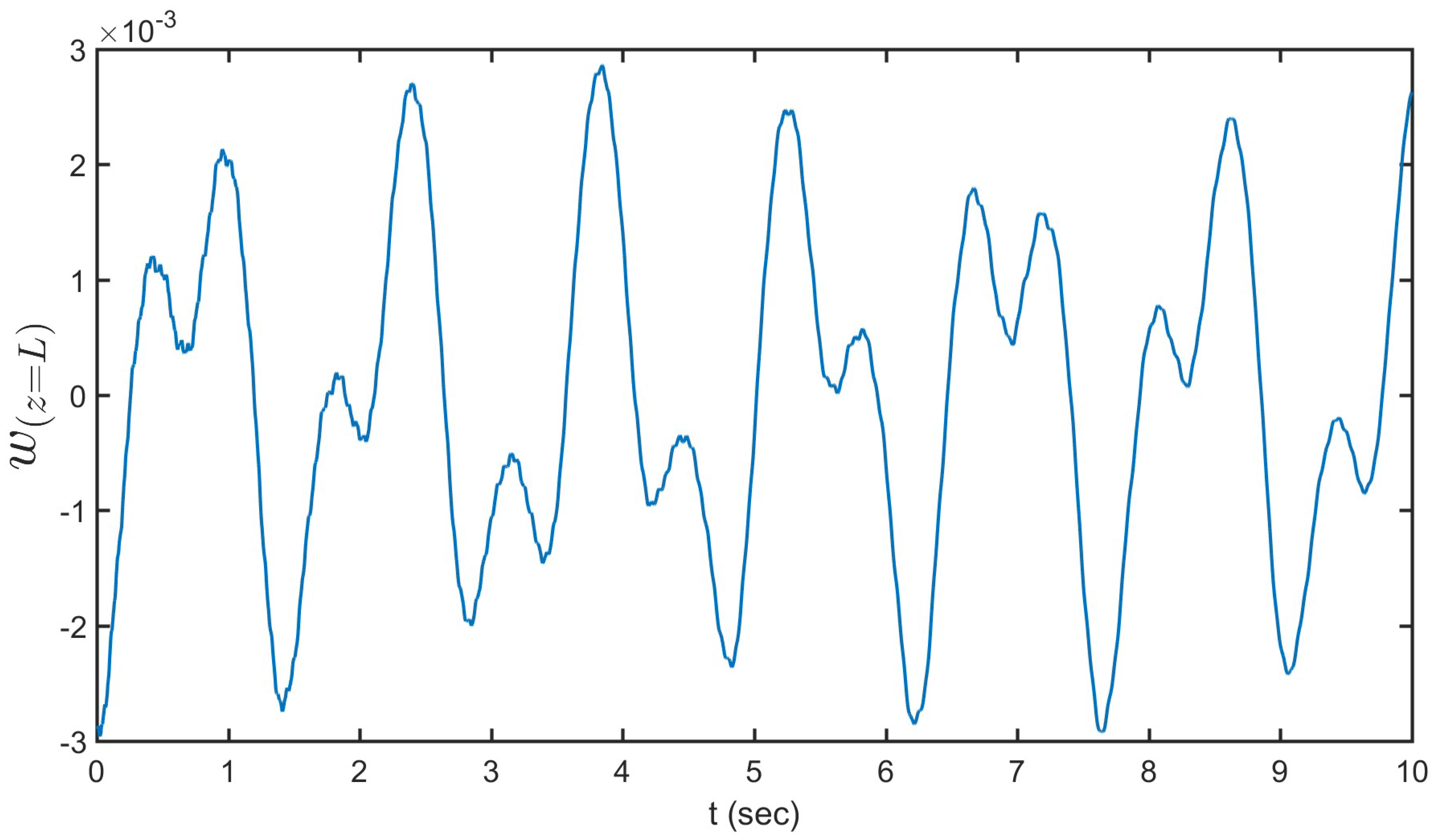
The sets of governing equations are rearranged in state space formulation and solved by Runge–Kutta time integration in MATLAB with Δt = 10−4 s. Figure 5 illustrates the tip displacement versus time. Initial condition considered here is the stationary case, with four Newtons tip force. The figure shows the maximum downward deflection of the beam is 3 mm. Figure 5 also shows that in steady conditions beam tip deflection started from 3 mm with two small oscillations in each period. The classical laminated plate theory gives the relationships among the plate bending moments, torsional moment and curvatures. The dimensionless coupling term here is small, where EI, GJ and K are bending stiffness about the y-axis, torsion stiffness and bending–torsion coupling stiffness, respectively. Different modes of operation lead to a wide range of frequencies, which are partially visible for example in the fluid forces acting on the structure.
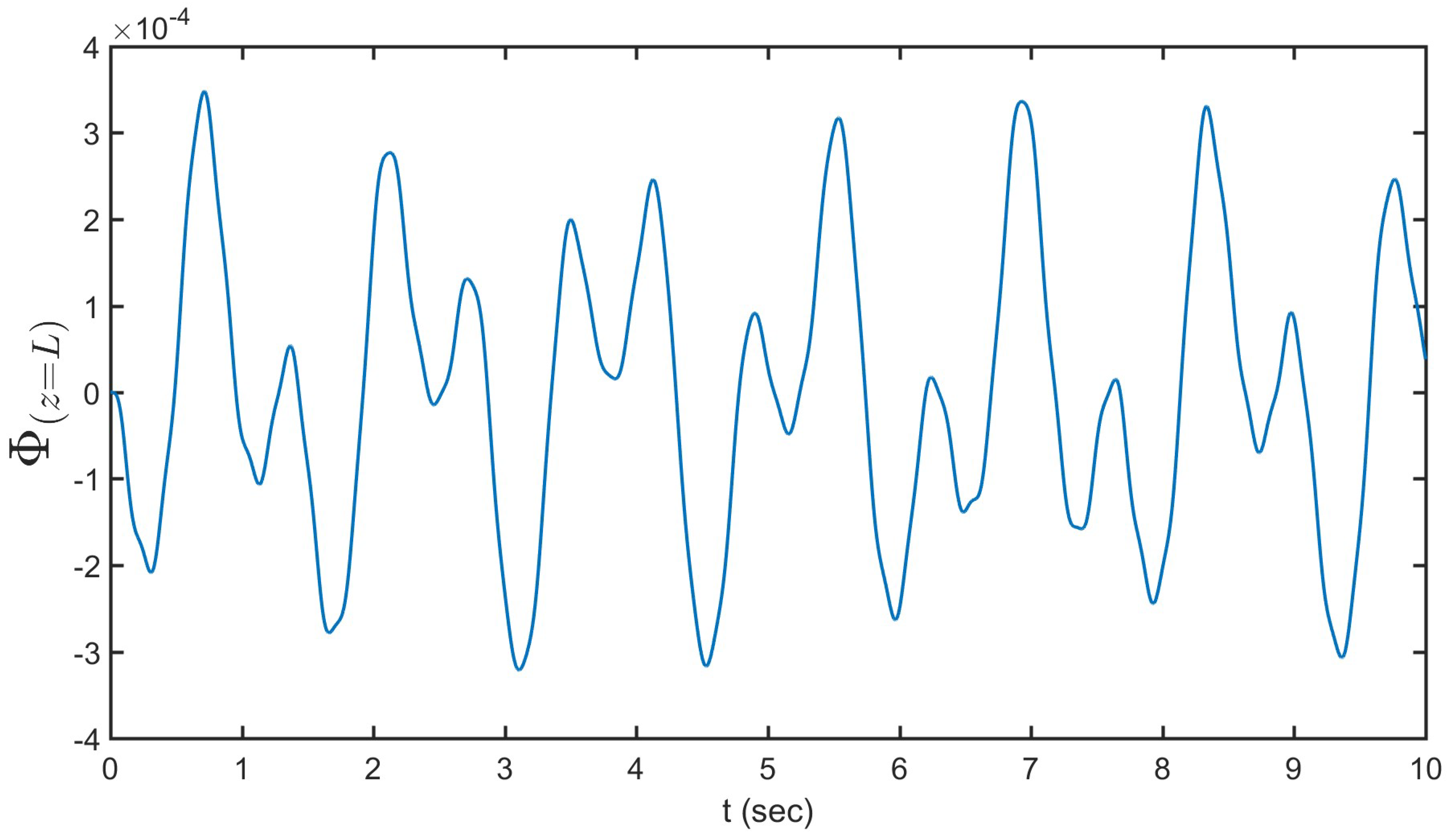
Angular deflection versus time graph for a vibrating cantilever beam subjected to the initial conditions can show the effect of bending motion on rotational mode. The tip torsion versus time is shown in Figure 6. As shown, the amplitude of orientation oscillation orientation of the sloshing vessel becomes larger with time. This is because the cylindrical shape of the vessel reduces resistance from the fluid flow so that the increasing deformation due to the time evolution leads to the reduction of the resistance in the vessel motion. The figure shows steady behavior started from equilibrium with two small oscillations in each period. In steady conditions, beam tip torsion started from zero degrees with two small oscillations in each period where the maximum reaches to 0.0003 radians.
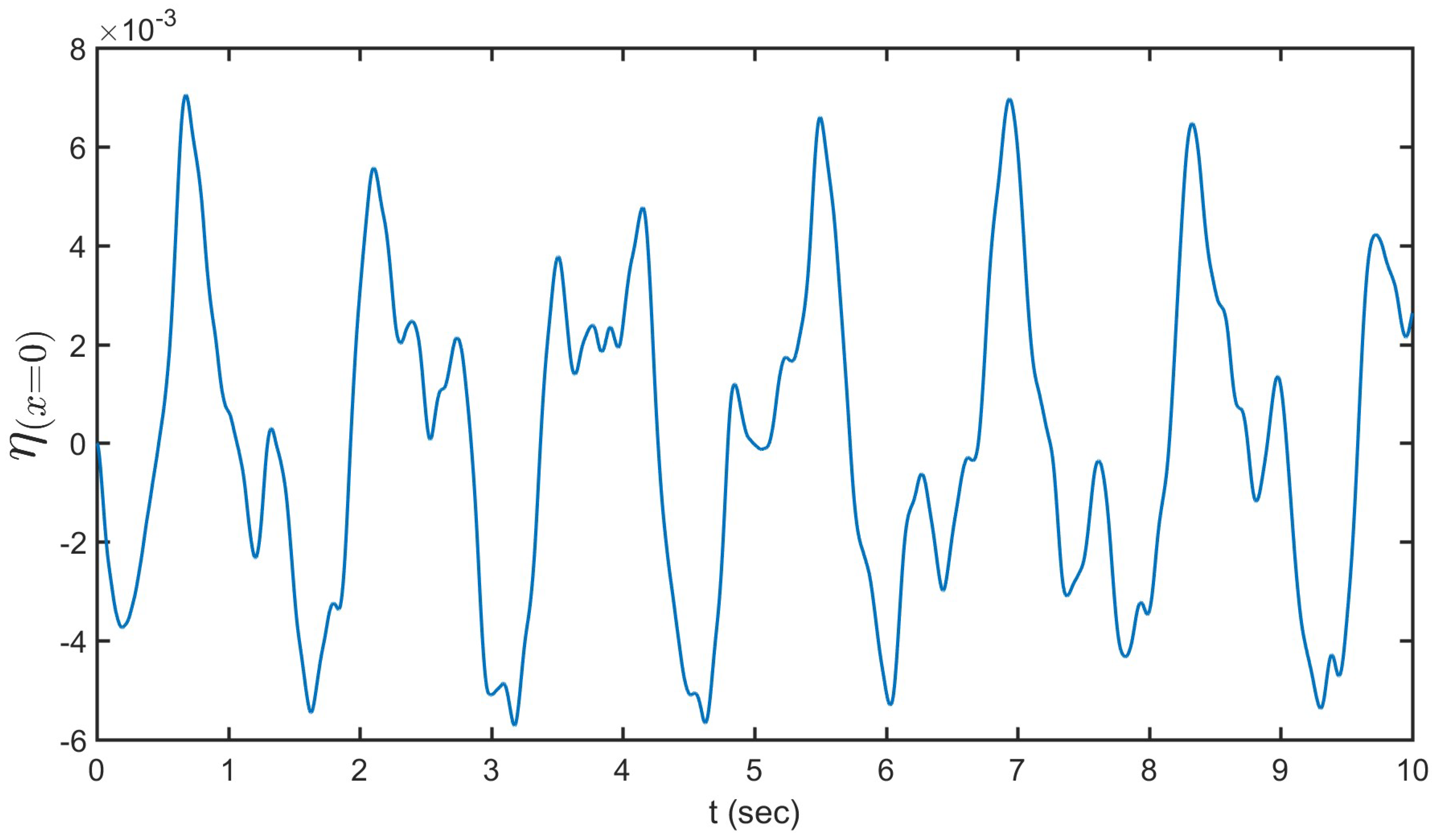
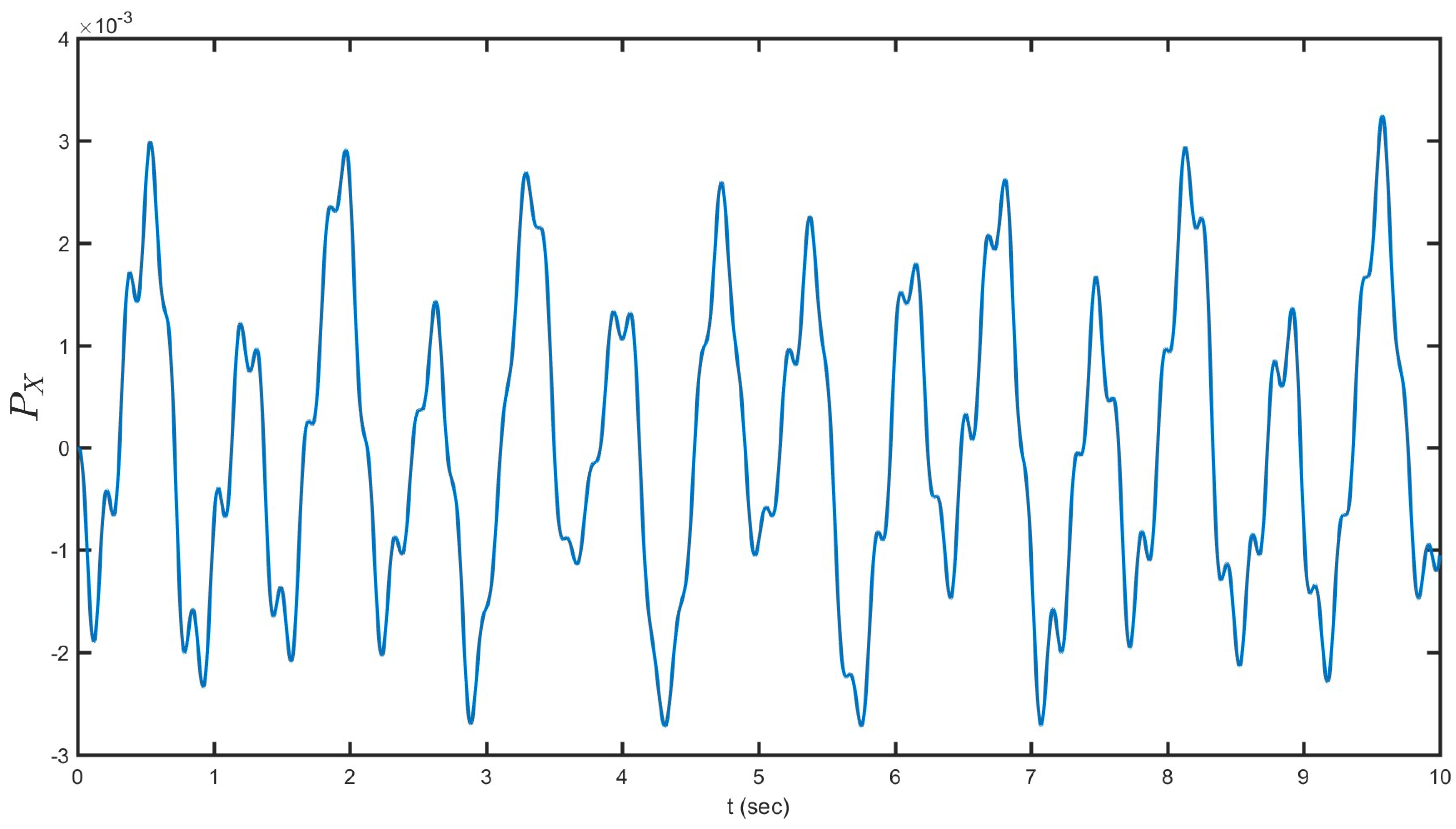
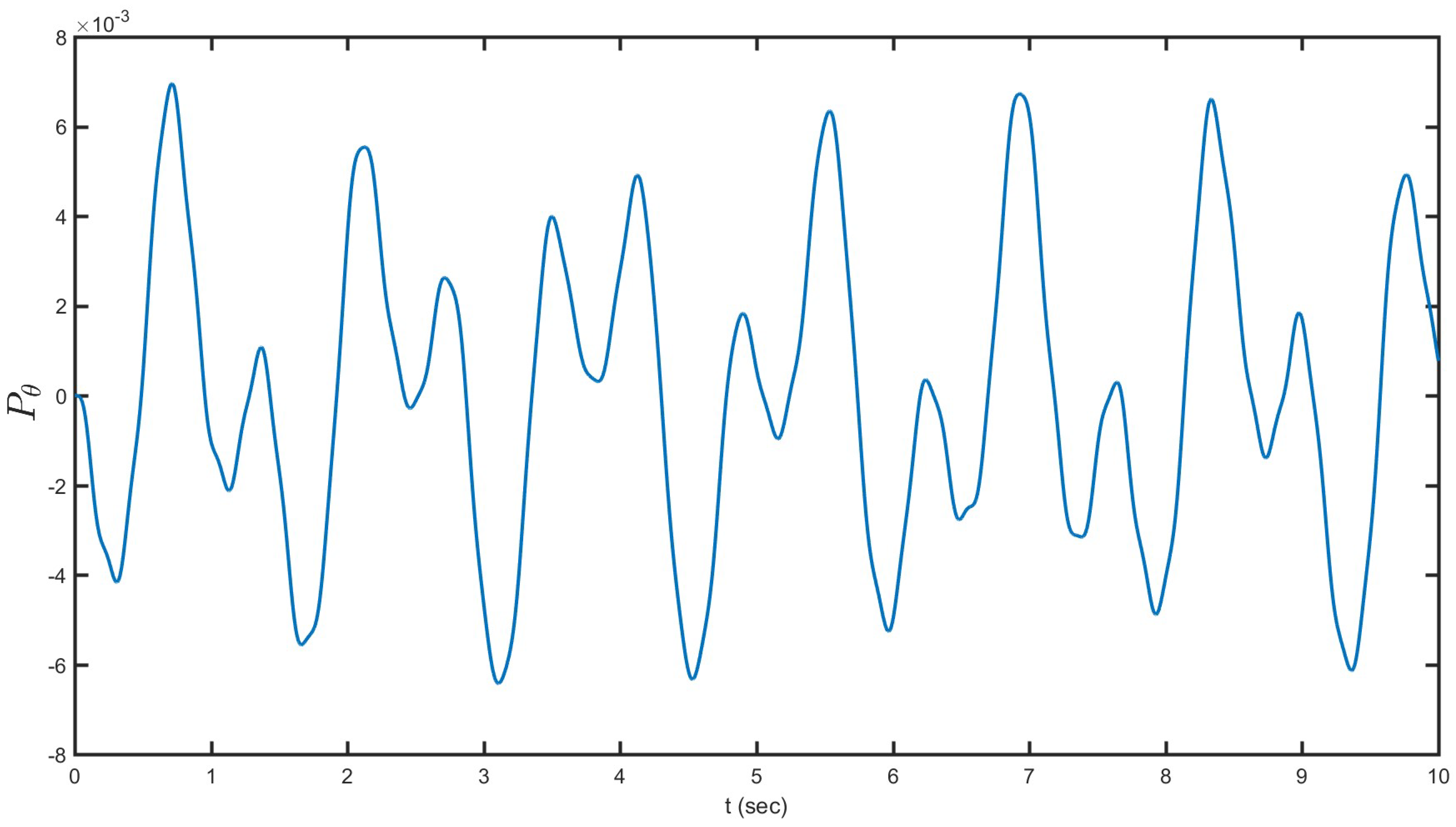
Figure 7 shows the depictions of the elevation of the water in the sloshing tank at the left wall versus time. The liquid begins in still condition and is energized utilizing symphonious voltages for the piezoelectric patches, with a recurrence near the main characteristic recurrence of sloshing. Figure 7 demonstrates the outcome after 10 s of recreation. As shown, the direct and nonlinear reenactments correspond and the state of the waves is similar to the primary modular bending of the liquid. Figure 8 presents the nonlinear horizontal momentum of the fluid versus time. The fluid starts in still condition and is stimulated using symphonious voltages for the piezoelectric patches, with a repeat close to the principle trademark repeat of sloshing. The maximum value of momentum fluctuations is 0.006 duration of motions on the sloshing phenomena in water tanks. Figure 9 reveals time dependency of the fluid angular momentum. The role of the rotational mode is stabilizing the coupling between fluid and structure. The smoothness of the liquid nonlinear conduct influences the basic mode reaction, lessening the amplitude of the vibrations. The vessel is moved by the piezoelectric wafers and the water reacts to it. The torsion mode was made a degree of freedom to release the energy of the system in the rotational degree of freedom and help maintain a stable coupling between fluid and structure.
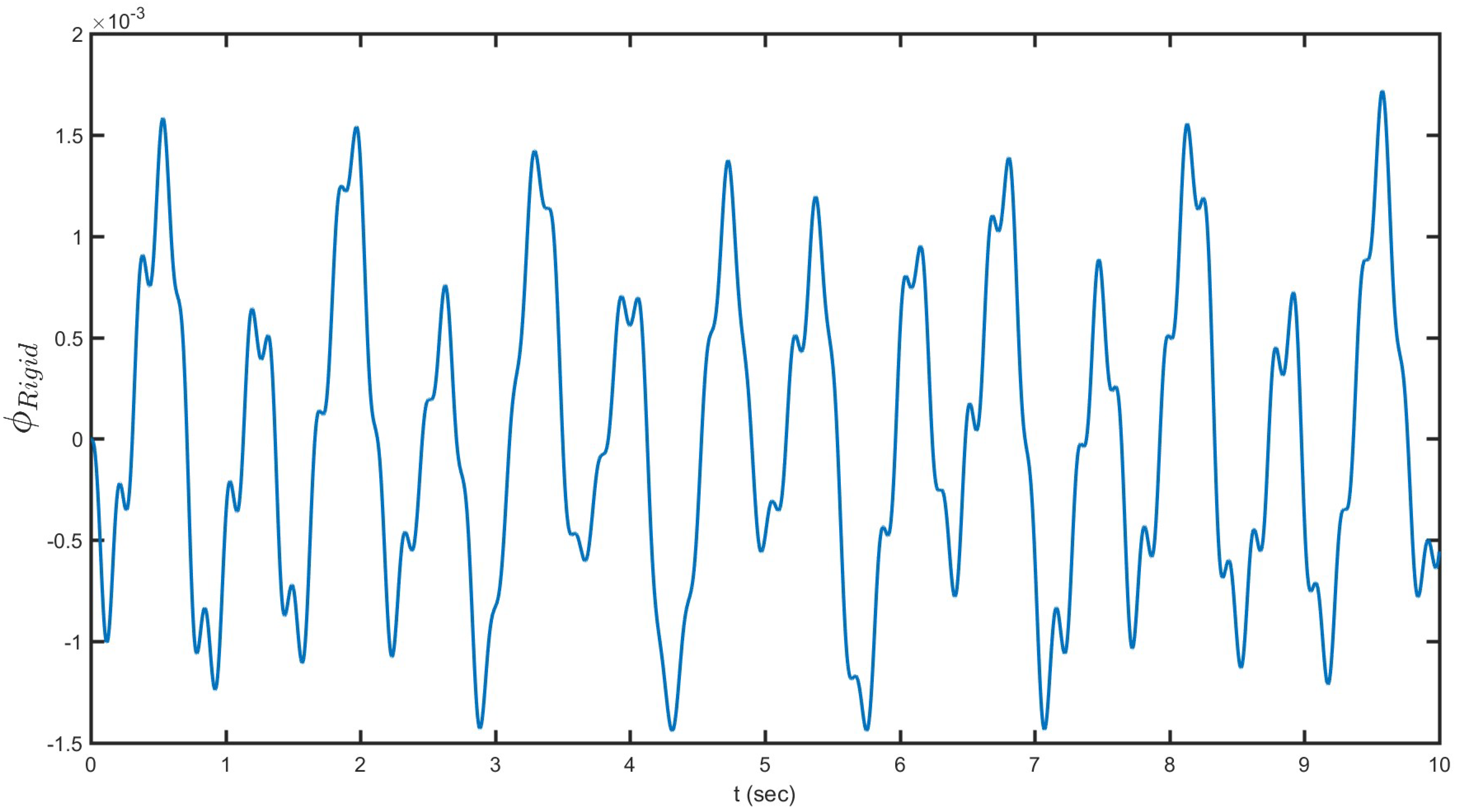
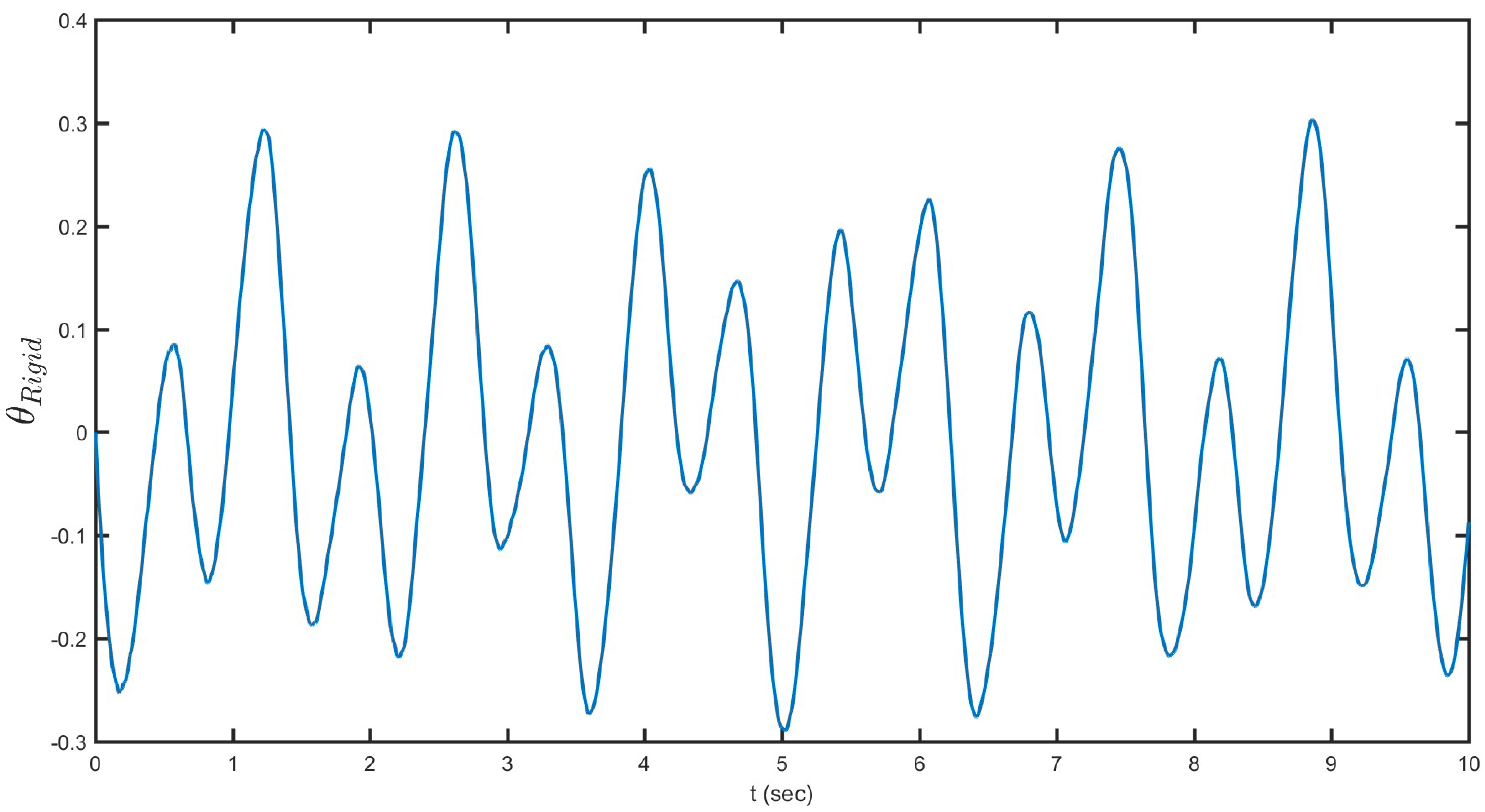
Figure 10 illustrates the rigid-body position versus time. Similar to Figure 5, it demonstrates the time reaction of the tip speed of the bar for these same reenactments. From the momentum equation in the inertial reference system, this phase lag evolves with slow time dynamics. Increasing torsional stiffness increases lateral stability. On the other hand, similar to the horizontal displacement, the time histories for rotation were obtained. Figure 11 displays rigid-body torsion versus time. In the sloshing–structure simulation shown in Figure 11, same as Figure 6, the level of torsion is low in comparison with the bending mode. The vessel is moved by the piezoelectric wafers and the water reacts to it. The torsion mode was made a degree of freedom to release the energy of the system in the rotational degree of freedom. The values calculated by Euler–Bernoulli theory completely prove that for the current study the bending can be considered to act independently in this case, well higher than that computed by the coupled Euler–Saint Venant bending–torsion theory. Although the Euler–Bernoulli theory would predict correctly the dynamics of the beam in Figure 11, the bending–torsion coupling effects cannot be neglected when applying random loads.
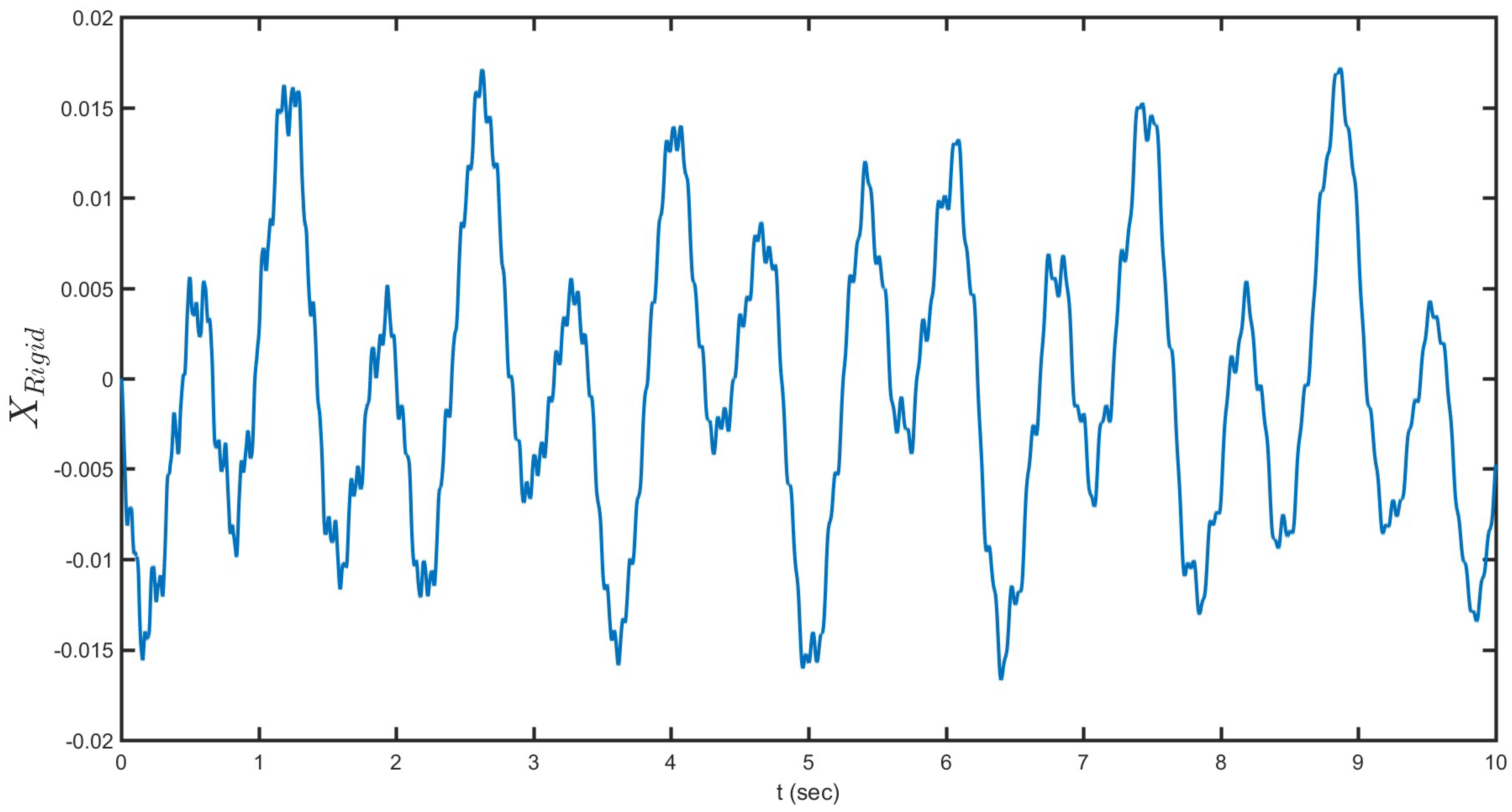
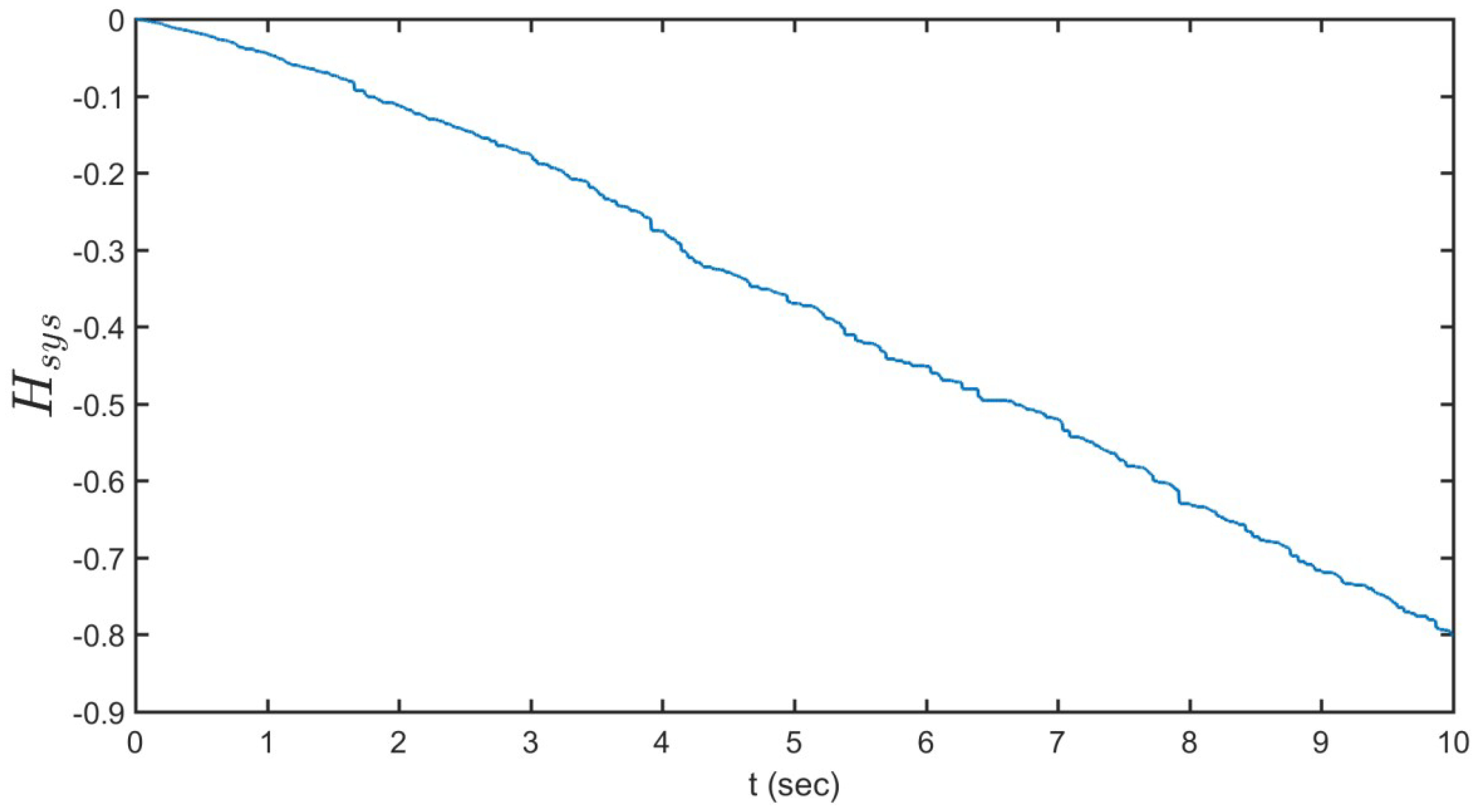
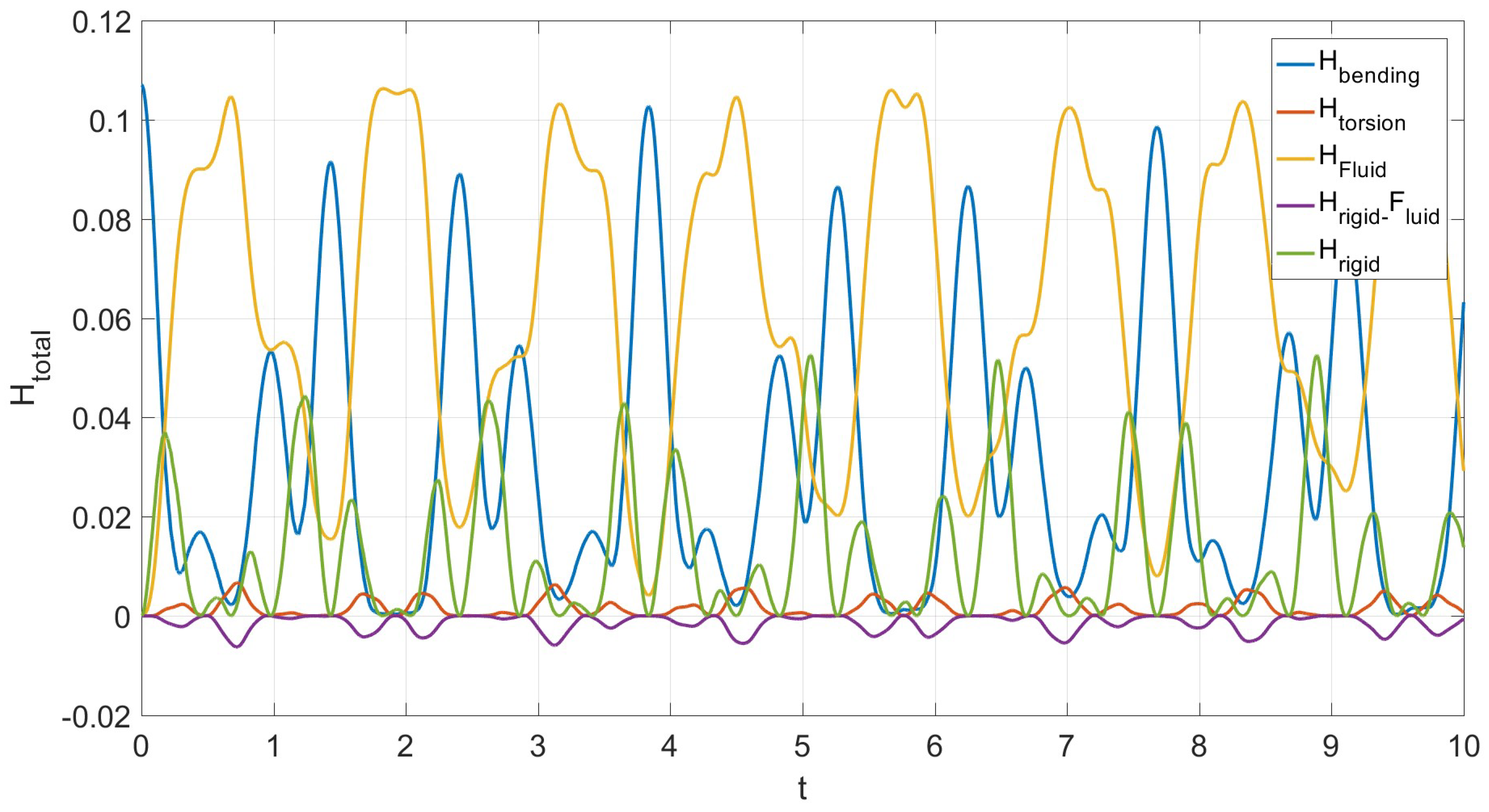
Figure 12 depicts rigid-body bending versus time. Simulating such a complex phenomenon, related to bending rotations of the beam, reveals the higher level of the bending in comparison with the torsion and smoothness of this motion because of the sloshing coupling. This quasi-periodicity can also be confirmed by looking at the predicted motion depicted in Figure 12. This effort sought to measure the dynamic nonlinear bending response of a cantilever beam. That shows the Euler theory for bending and Saint Venant theory for torsion are sufficient for current analysis. Note that, in most of the three-dimensional numerical datasets (see Figure 5, Figure 6, Figure 7, Figure 8, Figure 9, Figure 10, Figure 11 and Figure 12), the periodic motion is predicted. Figure 13 portrays percent change of the Hamiltonian of the system versus time. A small decrease of the total Hamiltonian of the system shows the general conservative for of the current system with low damping ratio. Notice that a very decent concurrence with test results was obtained. For the 75% filling proportion, the Hamiltonian of the system decrease by time. Figure 14 exposes the variation of the Hamiltonian of the sub-systems versus time. As shown, most energy is distributed between the fluid and bending modes with a 90-degree phase difference. The next order is the rigid-body motion. The lowest energies relate to the torsion of the system and rigid–fluid coupling.
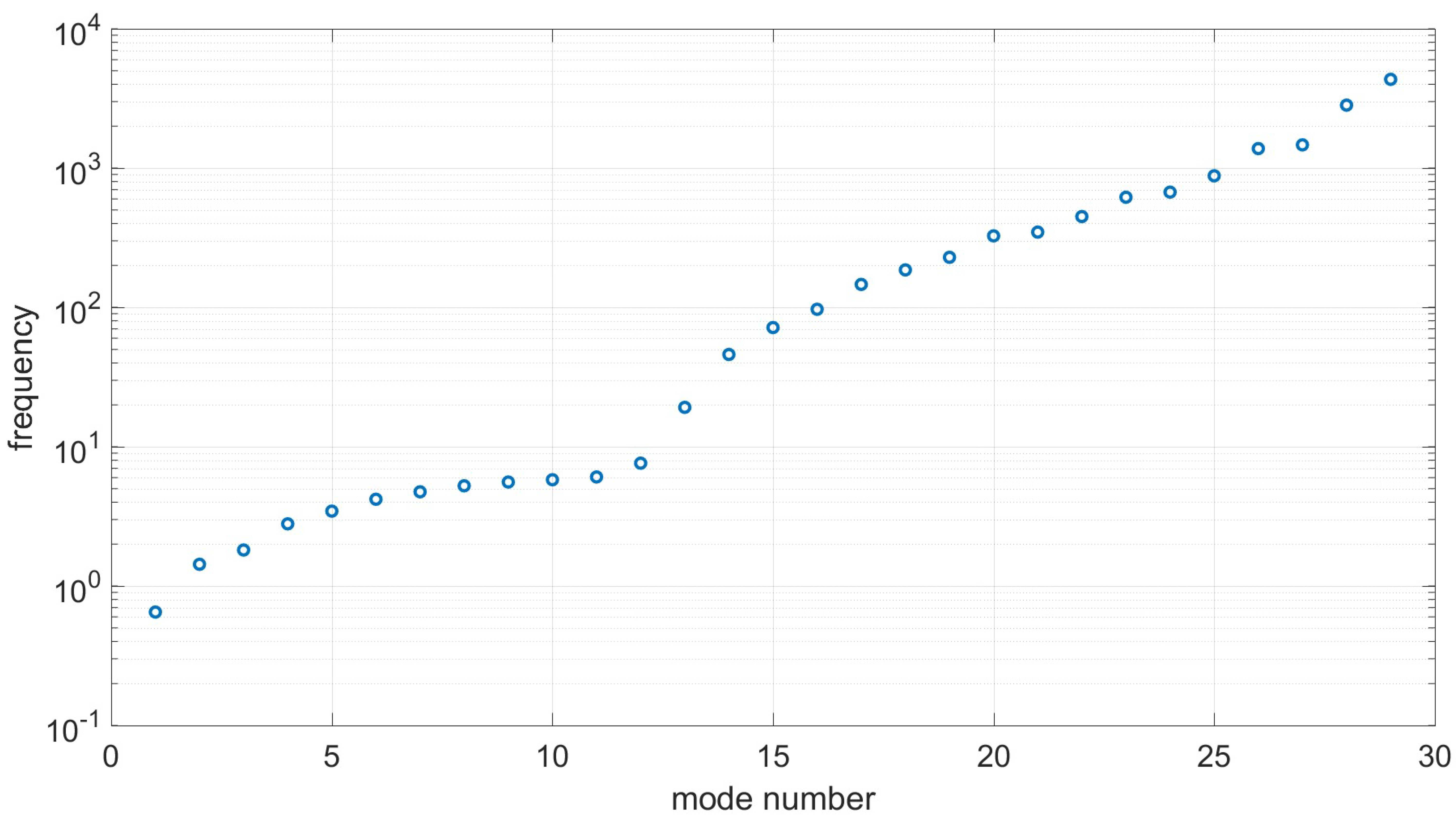
A result of the fully coupled system exemplifies in Figure 15 essential response frequencies of the system. The presented eigenvalues of the coupled system were obtained for filling ratio of 75 percent. The initial five modes are basically because of the coupling between the sloshing elements and the principal bending method of the structure. The sixth mode is commanded by the torsion elements. The seventh and eighth modes are bending modes. The liquid element additionally presents modes that are symmetric regarding the focal point of the tank. As can be seen in Figure 15, the first five normal modes are pure sloshing modes and the sixth normal mode is fundamental torsional mode when the effect of bending–torsion coupling is ignored. If the effect of bending–torsion coupling is considered, there is no strong coupling between bending and torsional displacements for the first six modes, since the sixth mode remains the fundamental torsional mode. Figure 15 shows that, although the bending–torsion coupling does not significantly affect the natural frequencies of sloshing, there can be appreciable differences in the mode shapes.
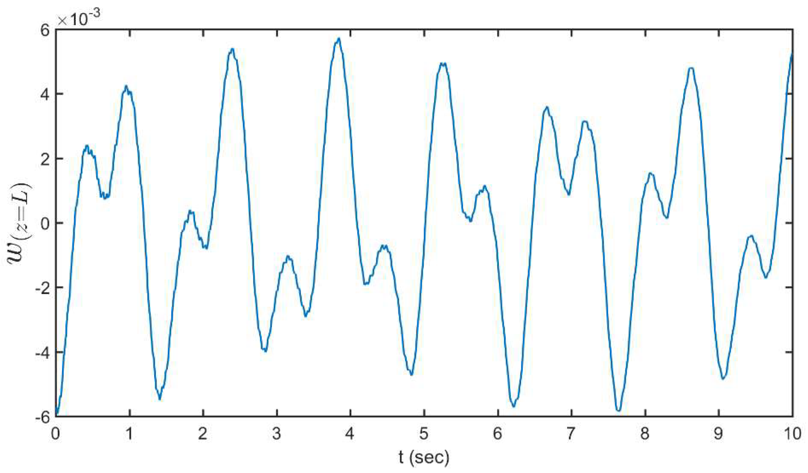
Figure 16 illustrates the tip displacement versus time. Initial condition considered here is the stationary case, with eight Newtons tip force. The figure shows maximum downward deflection of the beam is 6 mm with significantly larger deformations of the flexible structure. In steady conditions, beam tip deflection started from −6 mm with two small oscillations in each period. The similarity of Figure 5 and Figure 16 in profile shape illustrate that the system behavior is still linear in this limit.
4. Conclusions
An improvement of the port-Hamiltonian model of fluid sloshing coupled by structure motion was performed in this study. A new method to simulate the nonlinear effects of sloshing in confined vessels is presented. A set of governing equations including the shallow water equations in the one-dimensional case and bending and torsion of a beam are solved by Runge–Kutta time integration. This paper offers a modified shallow water equation which leads to a proper distribution in each computational cell, which prevents numerical errors in frequency response analysis of the system and maintaining continuity condition. The essential enthusiasm of utilizing this formalism, with regards to this work, is that it gives an efficient, secluded approach for demonstrating complex multi-material science marvels. Especially in contrast to past work utilizing shallow water conditions for the reenactment of sloshing in moving compartments, this paper expressly characterizes information and yields association ports that can be utilized for coupling components of an unpredictable framework in a simple and methodical way. The main contributions of this paper are the following:
- A new model for rotating–translating shallow water equations in moving containers is offered within the port-Hamiltonian equations.
- The suggested model was used to solve a fluid–structure interaction problem, which includes a piezoelectric actuator on a flexible beam (bending element and torsional element), and a rigid vessel. Each subsystem was considered within the port-Hamiltonian equations and coupled using the interaction ports.
Funding
This research received no external funding.
Conflicts of Interest
The author declares no conflict of interest.
References
- Molin, B.; Remy, F. Experimental and numerical study of the sloshing motion in a rectangular tank with a perforated screen. J. Fluids Struct. 2013, 43, 463–480. [Google Scholar] [CrossRef]
- Nicolici, S.; Bilegan, R.M. Fluid structure interaction modeling of liquid sloshing phenomena in flexible tanks. Nucl. Eng. Des. 2013, 258, 51–56. [Google Scholar] [CrossRef]
- Shadloo, M.S.; Oger, G.; le Touzé, D. Smoothed particle hydrodynamics method for fluid flows, towards industrial applications: Motivations, current state, and challenges. Comput. Fluids 2016, 136, 11–34. [Google Scholar] [CrossRef]
- Zhang, Z.; Qiang, H.; Gao, W. Coupling of smoothed particle hydrodynamics and finite element method for impact dynamics simulation. Eng. Struct. 2011, 33, 255–264. [Google Scholar] [CrossRef]
- Chen, B.F.; Nokes, R. Time-independent finite difference analysis of fully non-linear and viscous fluid sloshing in a rectangular tank. J. Comput. Phys. 2005, 209, 47–81. [Google Scholar] [CrossRef]
- Koutandos, E.; Prinos, P.; Gironella, X. Floating breakwaters under regular and irregular wave forcing: Reflection and transmission characteristics. J. Hydraul. Res. 2005, 43, 174–188. [Google Scholar] [CrossRef]
- Wei, Z.; Faltinsen, O.M.; Lugni, C.; Yue, Q. Sloshing-induced slamming in screen-equipped rectangular tanks in shallow-water conditions. Phys. Fluids 2015, 27, 032104. [Google Scholar] [CrossRef]
- Monaghan, J.J. Smoothed particle hydrodynamics. Ann. Rev. Astron. Astrophys. 1992, 30, 543–574. [Google Scholar] [CrossRef]
- Fatehi, R.; Shadloo, M.S.; Manzari, M.T. Numerical investigation of two-phase secondary kelvin-helmholtz instability. Proc. Inst. Mech. Eng. Part C 2013. [Google Scholar] [CrossRef]
- Benson, D.J. Computational methods in Lagrangian and Eulerian hydrocodes. Comput. Methods Appl. Mech. Engrg. 1992, 99, 235–394. [Google Scholar] [CrossRef]
- Rahmat, A.; Tofighi, N.; Shadloo, M.S.; Yildiz, M. Numerical simulation of wall bounded and electrically excited Rayleigh–Taylor instability using incompressible smoothed particle hydrodynamics. Colloids Surfaces A Physicochem. Eng. Asp. 2014, 460, 60–70. [Google Scholar] [CrossRef]
- Monaghan, J.J. Smoothed particle hydrodynamics. Rep. Prog. Phys. 2005, 68, 1703–1759. [Google Scholar] [CrossRef]
- Libersky, L.D.; Petschek, A.G. Smooth Particle Hydrodynamics with Strength of Materials. In Proceedings of the Next Free-Lagrange Conference, Moran, WY, USA, 3–7 June 1990; pp. 248–257. [Google Scholar]
- Benz, W.; Asphaug, E. Simulations of brittle solids using smoothed particle hydrodynamics. Comput. Phys. Commum. 1995, 87, 253–265. [Google Scholar] [CrossRef]
- Monaghan, J.J. SPH without a tensile instability. J. Comput. Phys. 2000, 159, 290–311. [Google Scholar] [CrossRef]
- Libersky, L.D.; Randles, P.W.; Carney, T.C.; Dickinson, D.L. Recent improvements in SPH modeling of hypervelocity impact. Int. J. Impact Eng. 1997, 20, 525–532. [Google Scholar] [CrossRef]
- Johnson, G.R.; Stryk, R.A.; Beissel, S.R. SPH for high velocity impact computations. Comput. Methods Appl. Mech. Engrg. 1996, 139, 347–373. [Google Scholar] [CrossRef]
- Johnson, G.R. Linking of Lagrangian particle methods to standard finite element methods for high velocity impact computations. Nucl. Eng. Des. 1994, 150, 265–274. [Google Scholar] [CrossRef]
- Attaway, S.W. Coupling of smoothed particle hydrodynamics with the finite element method. Nucl. Eng. Des. 1994, 150, 199–205. [Google Scholar] [CrossRef]
- Fernández-Méndez, S.; Bonet, J.; Huerta, A. Continuous blending of SPH with finite elements. Comput. Struct. 2005, 83, 1448–1458. [Google Scholar] [CrossRef] [Green Version]
- Yu, Y.; Ma, N.; Fan, S.; Gu, X. Experimental and numerical studies on sloshing in a membrane-type LNG tank with two floating plates. Ocean Eng. 2017, 129, 217–227. [Google Scholar] [CrossRef]
- Kotyczka, P.; Maschke, B. Discrete port-Hamiltonian formulation and numerical approximation for systems of two conservation laws. Automatisierungstechnik 2017, 65, 308–322. [Google Scholar] [CrossRef]
- Cardoso-Ribeiro, F.L.; Matignon, D.; Pommier-Budinger, V. A port-Hamiltonian model of liquid sloshing in moving containers and application to a fluid-structure system. J. Fluids Struct. 2017, 69, 402–427. [Google Scholar] [CrossRef]
- Ibrahim, R.A. Liquid Sloshing Dynamics; Cambridge University Press: Cambridge, UK, 2005. [Google Scholar]
- Lasiecka, I.; Tuffaha, A. Boundary feedback control in fluid-structure interactions. In Proceedings of the 47th IEEE Conference on Decision Control, Cancun, Mexico, 9–11 December 2008; pp. 203–208. [Google Scholar]
- Petit, N.; Rouchon, P. Dynamics and solutions to some control problems for water-tank systems. IEEE Trans. Autom. Control 2002, 47, 594–609. [Google Scholar] [CrossRef] [Green Version]
- Pommier-Budinger, V.; Richelot, J.; Bordeneuve-Guib, J. Active control of a structure with sloshing phenomena. In Proceedings of the IFAC Conference on Mechatronic Systems, Berkeley, CA, USA, 9–11 December 2006. [Google Scholar]
- Coron, J.-M. Local controllability of a 1-D tank containing a fluid modeled by the shallow water equations. ESAIM Control Optim. Calc. Var. 2002, 8, 513–554. [Google Scholar] [CrossRef] [Green Version]
- Prieur, C.; de Halleux, J. Stabilization of a 1-D tank containing a fluid modeled by the shallow water equations. Syst. Control Lett. 2004, 52, 167–178. [Google Scholar] [CrossRef]
- Robu, B. Active Vibration Control of a Fluid/Plate System. Ph.D. Thesis, University of Toulouse, Toulouse, France, December 2010. [Google Scholar]
- van der Schaft, A.J.; Jeltsema, D. Port-Hamiltonian Systems Theory: An introductory Overview; Trends Controls: Horsham, UK, 2014; pp. 173–378. [Google Scholar]
- Robu, B.; Baudouin, L.; Prieur, C.; Arzelier, D. Simultaneous H∞ Vibration Control of Fluid/Plate System via Reduced-Order Controller. IEEE Trans. Control Syst. Technol. 2012, 20, 700–711. [Google Scholar] [CrossRef]
- Cardoso-Ribeiro, F.L.; Pommier-Budinger, V.; Schotte, J.-S.; Arzelier, D. Modeling of a coupled fluid-structure system excited by piezoelectric actuators. In Proceedings of the 2014 IEEE/ASME International Conference on Advanced Intelligent Mechatronics, Besançon, France, 8–11 July 2014; pp. 216–221. [Google Scholar]
- Cardoso-Ribeiro, F.L.; Matignon, D.; Pommier-Budinger, V. Control design for a coupled fluid-structure system with piezoelectric actuators. In Proceedings of the 3rd CEAS EuroGNC, Toulouse, France, 13–15 April 2015. [Google Scholar]
- Ardakani, H.A.; Bridges, T.J. Dynamic coupling between shallow-water sloshing and horizontal vehicle motion. Eur. J. Appl. Math. 2010, 21, 479–517. [Google Scholar] [CrossRef]
- Ardakani, H.A.; Bridges, T.J. Shallow-water sloshing in vessels undergoing prescribed rigid-body motion in three dimensions. J. Fluid Mech. 2011, 667, 474–519. [Google Scholar] [CrossRef]
- Hamroun, B.; Lefevre, L.; Mendes, E. Port-based modelling and geometric reduction for open channel irrigation systems. In Proceedings of the 46th IEEE Conference on Decision and Control, New Orleans, LA, USA, 12–14 December 2007; pp. 1578–1583. [Google Scholar]
- Hamroun, B.; Dimofte, A.; Lefèvre, L.; Mendes, E. Control by Interconnection and Energy-Shaping Methods of Port Hamiltonian Models. Application to the Shallow Water Equations. Eur. J. Control 2010, 16, 545–563. [Google Scholar] [CrossRef] [Green Version]
Figure 1.
Schematic of the system.

Figure 2.
Definitions of forces and deflections in system.

Figure 3.
Two-dimensional model of moving vessel.

Figure 4.
Basis functions.

Figure 5.
The tip displacement versus time.

Figure 6.
The tip torsion versus time.

Figure 7.
The elevation at the left wall versus time.

Figure 8.
Fluid horizontal momentum versus time.

Figure 9.
Fluid angular momentum versus time.

Figure 10.
Rigid-body position versus time.

Figure 11.
Rigid-body torsion versus time.

Figure 12.
Rigid-body bending versus time.

Figure 13.
Percent change of the Hamiltonian of the system versus time.

Figure 14.
The variation of the Hamiltonian of the sub-systems versus time.

Figure 15.
Essential frequencies of the system.

Figure 16.
The tip displacement versus time.


Table 1.
Parameters of the system.
| Parameter | Value | Unit | Description |
|---|---|---|---|
| Lb | 1.36 | m | Plate length |
| wb | 0.16 | m | Plate width |
| tb | 0.005 | m | Plate thickness |
| ρb | 2970 | kg·m−3 | Plate density |
| Eb | 75 | GPa | Plate Young modulus |
| νb | 0.33 | - | Plate Poisson coefficient |
| Lpa | 0.14 | m | Actuator length |
| wpa | 0.075 | m | Actuator width |
| tpa | 0.5 | mm | Actuator thickness |
| ρpa | 7800 | kg·m−3 | Actuator density |
| Epa | 67 | GPa | Actuator Young modulus |
| νpa | 0.3 | - | Actuator Poisson coefficient |
| d31 | −210 | pm·V−1 | Actuator piezoelectric strain coefficient |
| Lps | 0.015 | m | Sensor length |
| wps | 0.025 | m | Sensor width |
| tps | 0.5 | mm | Sensor thickness |
| ρps | 7800 | kg·m−3 | Sensor density |
| Eps | 67 | GPa | Sensor Young modulus |
| νps | 0.3 | - | Sensor Poisson coefficient |
| cps | −9.6 | Nm−1V−1 | Sensor piezoelectric coefficient |
| xr | 1.28 | m | rigid body distance from clamp along z axis |
| Dout | 0.11 | m | Vessel exterior diameter |
| Din | 0.105 | m | Vessel interior diameter |
| Lout | 0.5 | m | Vessel outside length |
| Lin | 0.47 | m | Vessel inside length |
| ρ | 1180 | kg·m−3 | Vessel density |
| E | 4.5 | GPa | Vessel Young modulus |
| Doutring | 0.1445 | m | Fixation rings exterior diameter |
| Dinring | 0.11 | m | Fixation rings interior diameter |
| tring | 28.76 | mm | Fixation rings thickness |
| dring | 16.9 | mm | Fixation rings distance from plate mean axis |
| ρring | 2970 | kg·m−3 | Fixation rings density |
| Ering | 75 | GPa | Fixation rings Young modulus |
| mring | 588.6 | g | Total fixation ring masses |
| mtip | 313 | g | Tip masses |
| Ltip | 0.24 | m | Distance of tip masses from plate mean axis |
Table 2.
Hamiltonian of the parts of the system.
| Sub-system. | Type | Formula |
|---|---|---|
| Beam bending | Potential | |
| Kinetic | ||
| Beam Torsion | Potential | |
| Kinetic | ||
| Rotating–translating shallow water | Potential | |
| Kinetic |
Table 3.
Governing equations of the parts of the system.
| Sub- | Formula |
|---|---|
| Beam bending | |
| Beam Torsion | |
| Rotating–translating shallow water |
Table 4.
Boundary condition of the parts of the system.
| Sub- | Formula |
|---|---|
| Beam bending | |
| Beam Torsion | |
| Rotating–translating shallow water |
Table 5.
Comparison of the calculated natural frequency of the system with experiment.
| Filling Ratio | Previous [23] | Current | Experiment |
|---|---|---|---|
| 0.25 | 0.43 | 0.44 | 0.47 |
| 0.5 | 0.59 | 0.57 | 0.55 |
© 2018 by the author. Licensee MDPI, Basel, Switzerland. This article is an open access article distributed under the terms and conditions of the Creative Commons Attribution (CC BY) license (http://creativecommons.org/licenses/by/4.0/).
Share and Cite
MDPI and ACS Style
Abdollahzadeh Jamalabadi, M.Y. An Improvement of Port-Hamiltonian Model of Fluid Sloshing Coupled by Structure Motion. Water 2018, 10, 1721. https://doi.org/10.3390/w10121721
AMA Style
Abdollahzadeh Jamalabadi MY. An Improvement of Port-Hamiltonian Model of Fluid Sloshing Coupled by Structure Motion. Water. 2018; 10(12):1721. https://doi.org/10.3390/w10121721
Chicago/Turabian StyleAbdollahzadeh Jamalabadi, Mohammad Yaghoub. 2018. "An Improvement of Port-Hamiltonian Model of Fluid Sloshing Coupled by Structure Motion" Water 10, no. 12: 1721. https://doi.org/10.3390/w10121721
Note that from the first issue of 2016, this journal uses article numbers instead of page numbers. See further details here.