Hydrological Restoration and Water Resource Management of Siberian Crane (Grus leucogeranus) Stopover Wetlands
by
Haibo Jiang
1, 
Chunguang He
1,*,
Wenbo Luo
1,
Haijun Yang
1,
Lianxi Sheng
1,
Hongfeng Bian
1,* and
Changlin Zou
2 1
State Environmental Protection Key Laboratory of Wetland Ecology and Vegetation Restoration, Key Laboratory for Vegetation Ecology, Ministry of Education, Jilin Provincial Key Laboratory of Ecological Restoration and Ecosystem Management, Northeast Normal University, Changchun 130117, China
2
Momoge National Nature Reserve of Jilin, Baicheng 137000, China
*
Authors to whom correspondence should be addressed.
Water 2018, 10(12), 1714; https://doi.org/10.3390/w10121714
Submission received: 28 October 2018
/
Revised: 19 November 2018
/
Accepted: 20 November 2018
/
Published: 23 November 2018
(This article belongs to the Section Water Resources Management, Policy and Governance)
Abstract
:Habitat loss is a key factor affecting Siberian crane stopovers. The accurate calculation of water supply and effective water resource management schemes plays an important role in stopover habitat restoration for the Siberian crane. In this paper, the ecological water demand was calculated and corrected by developing a three-dimensional model. The results indicated that the calculated minimum and optimum ecological water demand values for the Siberian crane were 2.47 × 10⁸ m3~3.66 × 10⁸ m3 and 4.96 × 10⁸ m3~10.36 × 10⁸ m3, respectively, in the study area. After correction with the three-dimensional model, the minimum and optimum ecological water demand values were 3.75 × 10⁸ m3 and 5.21 × 10⁸ m3, respectively. A water resource management scheme was established to restore Siberian crane habitat. Continuous, area-specific and simulated flood water supply options based on water diversions were used to supply water. The autumn is the best season for area-specific and simulating flood water supply. These results can serve as a reference for protecting other waterbirds and restoring wetlands in semi-arid areas.
1. Introduction
Wetland degradation is the main factor underlying the decline of waterbirds and poses a serious threat to the health and subsistence of waterbirds [1]. Wetland restoration is an important mechanism to protect waterbird habitat [2]. Most of this study is focused on comparing hydrology, biology, and soil before and after restoring a wetland, as well as investigating approaches to wetland restoration [3,4,5,6,7]. The results indicate that hydrological conditions affect the structures and features of wetland animals, plants, and microorganisms, and play an important role in wetland restoration and management [8,9,10,11]. Hydrological restoration can be estimated by experience and calculated by models [12,13,14]. Combining the theories and methods of ecology and hydrology, ecological water demand has been widely used in wetland hydrological restoration [15,16,17]. However, most studies on ecological water demand are focused on river ecosystems, and studies on wetlands are limited [18,19]. The study on ecological water demand of wetland is focused on concept, qualitative analysis, and empirical method estimation. The quantitative evaluations of theoretical models and methods are relatively few [20,21]. The accuracy and feasibility of ecological water demand calculations have not been effectively corrected, resulting in negative effects on wetland restoration [22]. Scientific water supply schemes can result in effective restoration of wetlands [23,24].
The Siberian crane (Grus leucogeranus) is a large migrating waterbird, listed as a threatened species on the “red list” of the International Union for Conservation of Nature (IUCN). The global population of the Siberian crane is estimated to be approximately 4000 individuals. The eastern population is the largest, accounting for approximately 95% of the total number of Siberian cranes [25]. During their migration, the Siberian cranes stop at the Songnen Plain wetlands for 1–2 months to replenish their energy [26]. The Momoge National Nature Reserve (MNNR) is the main stopover site of the Siberian crane [27]. However, because of droughts and human activities, the wetland stopover sites in the MNNR have continuously diminished. Siberian cranes have not stopped in the area since 2007, whereas they had stopped there over the previous 25 years [22]. The loss of stopover habitat has seriously threatened the migration process of the Siberian cranes. The government of Jilin Province has enacted a water diversion project around the MNNR. In the present study, the Siberian crane stopover habitat is intended to be restored, basing on the project.
In this study, the relationship between Siberian crane number and wetland area was analyzed. The objectives of our study are following: (1) to calculate the minimum and optimum ecological water demand in the study area; (2) to correct the calculated water supply by a three-dimensional model; and (3) to develop an effective water resource management scheme.
2. Materials and Methods
2.1. Study Area
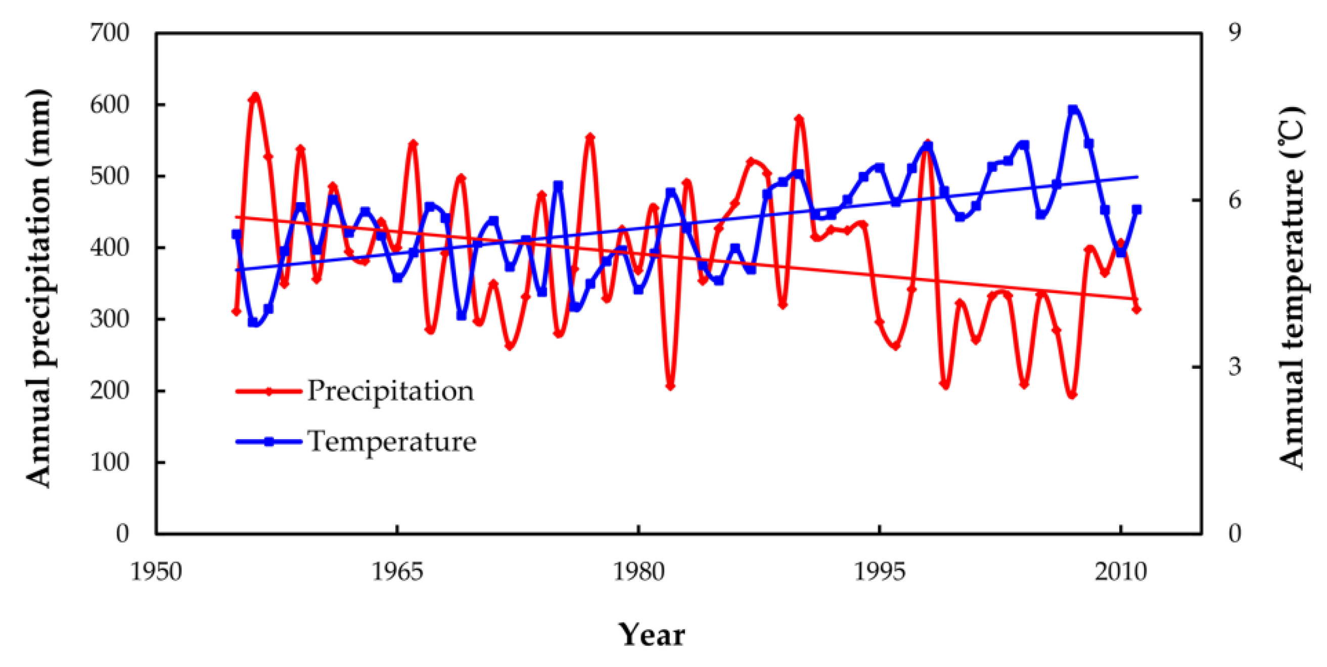
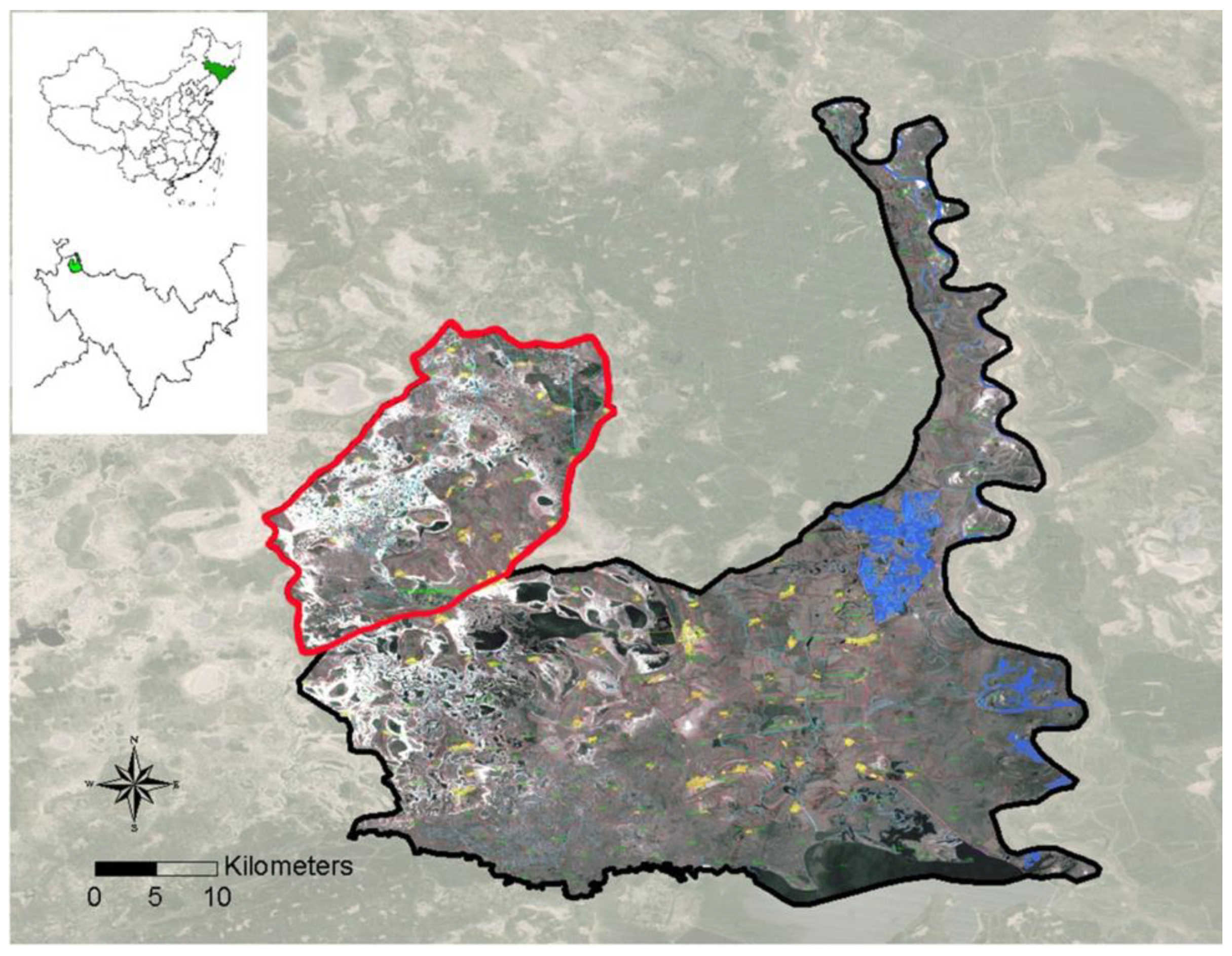
The MNNR (45°42′25″–46°18′0″ E, 123°27′0″–124°4′33″ N) is located in the Songnen Plain in China and covers an area of 1440 km2. It is one of the largest wetlands in northeast China. Most of the area contains shallow swamp, and it situated in a semiarid area with the continental monsoon climate of the north temperate zone [28]. Over the past 60 years, the annual precipitation, evapotranspiration, and mean temperature values were 385.69 mm, 1530.13 mm, and 4.97 °C, respectively. An increasing trend in the mean temperature and a decreasing trend in the annual precipitation have occurred in the nature reserve (Figure 1).
The study area is located in the western area of the MNNR, with an area of 300 km2 (Figure 2). The shallow water meadows of the study area are the main stopover habitat for the threatened Siberian crane.
2.2. Data Collection
2.2.1. Remote Sensing Data
Landsat Thematic Mapper (TM) and Landsat Earth Thematic Mapper (ETM) remote sensing images were obtained from the International Scientific Data Service Platform. The resolution of Landsat TM/ETM images is 30 m. The collection dates for these data were 5 July 1988, 25 June 1990, 29 May 1992, 10 October 1994, 12 October 1996, 3 September 1998, 1 May 1999, 5 October 2001, 17 October 2003, 8 October 2005, 16 October 2006, and 12 September 2007. Strips of TM images were repaired by ENVI 4.7 software, and then all remote images were calibrated. The resulting data were geo-referenced to the same coordinates using GPS information on the feature points, and a second-order polynomial transformation was performed with nearest-neighbor resampling using ArcGIS 9.3. The error of geo-referencing was ensured within a pixel. In addition, the landscape types in the study area were interpreted.
2.2.2. Siberian Crane Data
Siberian cranes stop at the MNNR from the beginning of April to the middle of May in the spring and from the middle of September to the beginning of November in autumn each year. During the stopover of the Siberian cranes, observers recorded the stopover number every two days. The observation time was from 08:00 to 10:00 h. The data were obtained at the MNNR in the spring from 1983 to 2007.
2.3. Model Calculation
2.3.1. Ecological Water Demand Calculation
Yang et al. proposed the calculation method of ecological water demand suitable for lake and wetland [29,30]. Ecological water demand includes plant water demand (wetland plant transpiration and plant water content), surface evaporation water demand (surface evaporation at Siberian crane stopover sites), wetland soil water demand (soil water capacity), waterfowl stopover site water demand (water demand for maintaining the growth and survival of Scirpus planiculmis and Siberian crane stopover and feeding), and water supply demand (supply underground water). Because the study area is in a water-scarce area, minimum and optimum water demands were analyzed in this paper. The minimum water demand is the lowest water demand for maintaining Siberian crane stopovers. The optimum water demand is the water demand that would improve the ecological environment of the wetland and make the area suitable to Siberian crane stopovers and feeding [29]. The ecological water demands can be calculated using the following equations [30].
where Wt is the ecological water demand for the Siberian crane (m3); Wp is the wetland plant water demand (m3); Wv is the surface evaporation water demand (m3); We is the wetland soil water demand (m3); Wh is the Siberian crane stopover habitat water demand (m3); Wu is the water supplement demand (m3); EP is the wetland plant evaporation (mm); A is the area of the study area (km2); E601 is the surface evaporation measured by E-601 evaporator; Av is the water area of the study area (km2); α is the field capacity; He is the soil thickness (m); Ae is the soil area of the study area (km2); β is the percentage of wetland surface area in study area; Hh is the optimal water level for Siberian crane stopovers (m); k is the permeability coefficient (m/d); and T is the time length (d).
2.3.2. Three-Dimensional Simulation for Water Supply
A 1:10,000 topographic map was vectored and attributed by R2 V based on WGS84 (World Geodetic System) for the coordinates of latitude and longitude. Spatial relationships and related attribution information for every element were saved, generating a Digital Line Graph (DLG). A two-dimensional spatial model was established. The Digital Elevation Model (DEM) for describing the spatial distribution of the regional geomorphic form was established after attributing contour lines. The three-dimensional visualization of the DEM model was developed using ArcView 3.3. The TM remote sensing image (September 2007) was fused with the satellite image, using ERDAS 8.5 software for inputting data and Dataprep for correcting the image. The Document Object Model (DOM) was established by matching image and digital height. The DLG, DEM, and DOM were stacked by ArcGIS 9.3 based on the 9 GPS feature points, generating a three-dimensional static model for Siberian crane stopover sites. To confirm the precision of the simulation, when the water level of study area border exceeds the elevation of the border in the process of simulation, the water will flow out from study area based on the difference in elevation (Figure 2).
The three-dimensional model was analyzed by ArcGIS 9.3, including transverse section analyses of 0.25 m to divide the drainage basin and calculate water levels for different water, slope, aspect and hydrology analyses to determine the flow direction, flow rate, fitting pattern and distribution of water network. In the process of the three-dimensional dynamic simulation, the water of the study area at time t can be calculated using the following equations:
where Wti is the water at ti time (m3); Wti−1 is the water at ti−1 time (m3); Wc is the water inflow from ti−1 to ti time (m3); Ww is the surface evaporation at ti time (subtract evaporation from precipitation, m3); Awi is the water area at ti time (calculate by ArcGIS 9.3, m2); is the water evaporation rate; Δt is the interval between ti−1 and ti time; Ws is the soaking soil evaporation (m3); Asi is the soaking soil area (calculate by ArcGIS 9.3, m2); ε is the soaking soil evaporation rate; Wu1 is the soil infiltration capacity before saturation (m3); δ1 is the soil infiltration coefficient before saturation; Wu2 is the soil infiltration capacity after saturation (m3); and δ2 is the soil infiltration coefficient before saturation.
3. Results and Discussion
3.1. Relationship between Siberian Crane Number and Wetland Area
The number of Siberian cranes in the spring from 1983 to 2006 is shown in Figure 3, with 200~800 Siberian cranes in the study area. However, there have been no Siberian crane stopovers at the study area since 2007. In 2007, the increase of water supply for human production activities (e.g., paddy field irrigation), the increase in temperature, and the decrease in precipitation (Figure 1) aggravated the degradation of wetlands, resulting in further reduction of wetland area. The reason for no stopovers is attributed to the poor hydrological conditions and drying of the wetlands. Therefore, Siberian cranes left the study area and went to stopover sites with good hydrological conditions.
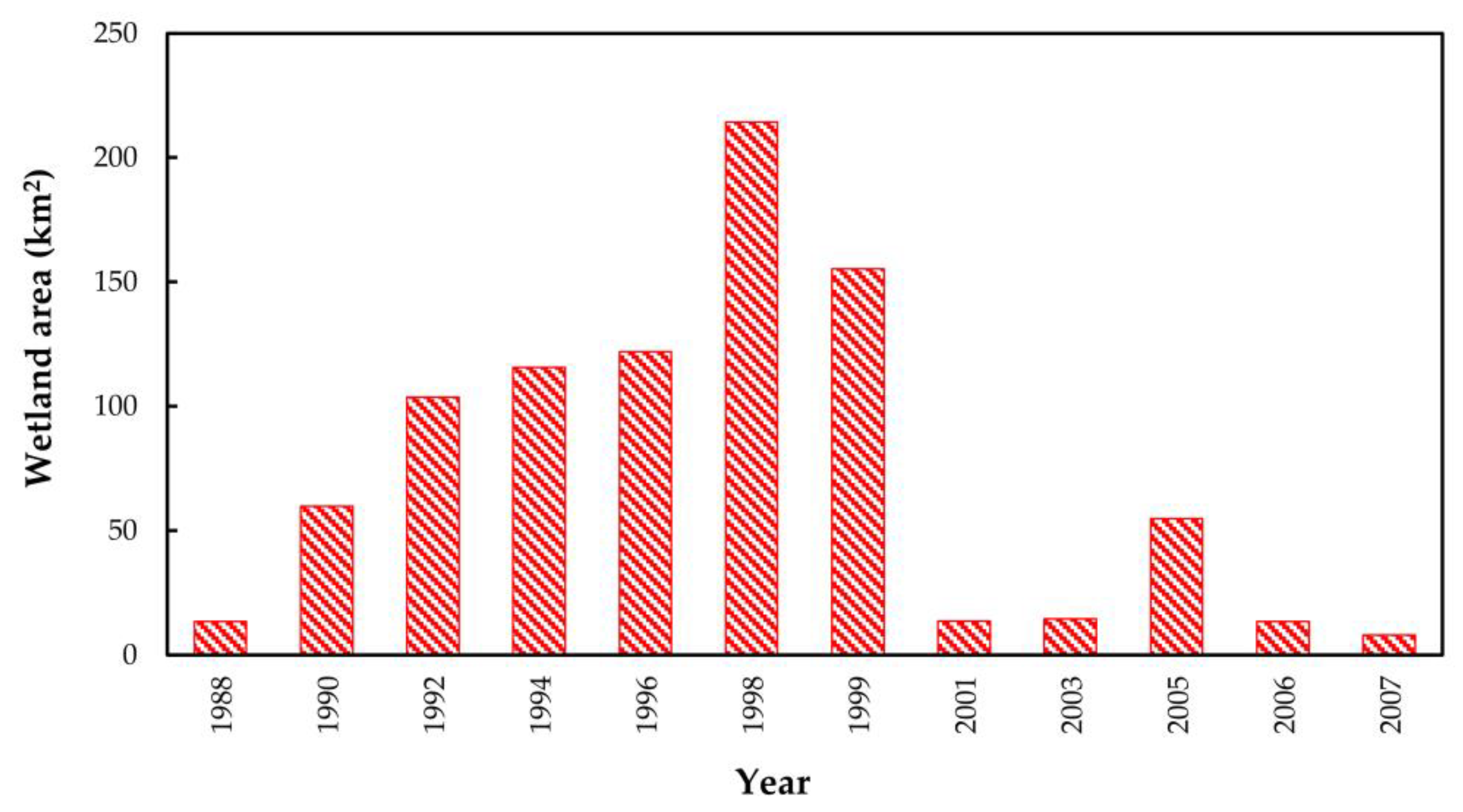
The wetland areas in the study area from 1988 to 2007 were interpreted from remote sensing images (Figure 4). The wetland area of the study area was relatively large from 1992 to 1999. Because of the large flood in 1998, the wetland area rapidly increased. However, in the following years, the wetland area substantially decreased. One of important reasons for the decrease was the continuous drought. The temperature increased and the precipitation decreased from 1999 (Figure 1), leading to a reduction in water inflow and an increment in water outflow in the study area.
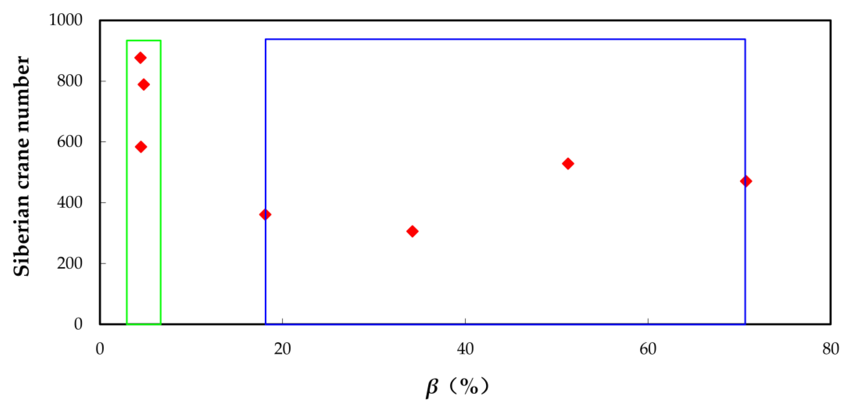
The relationship between the Siberian crane number and β value (the percentage of wetland surface area in study area) was determined (Figure 5). Because the wetland area was interpreted every summer or autumn, the hydrological conditions influenced the wetland area the following spring. Therefore, the Siberian crane number was selected from the spring, and the β value was selected from the previous year. The Siberian crane number in the Momoge wetland did not increase with an increasing β. When the β was approximately 4~7%, the Siberian crane number was 600~900. When the β increased, the Siberian crane number was stable (300~500). Furthermore, the distribution pattern of the Siberian crane was observed. The results show that when the Siberian crane number was 300~500, the distribution of the Siberian crane was dispersed; when the Siberian crane number was 600~900, the distribution of the Siberian crane was concentrated in the northeast of study area. The different distribution patterns are attributed to the persistent drought in the Songnen Plain starting in 2000 and unreasonable use of water resources by humans (such as water conservancy project, agricultural irrigation). The habitat for Siberian crane stopover sharply decreased, but the shallow water meadows of the study area can still provide some stopover sites for the Siberian crane. The number of Siberian crane stopovers at other wetlands in the Songnen Plain decreased, leading to the number of Siberian crane stopovers at the study area increasing. At the same time, the distribution of Siberian crane showed a concentration phenomenon.
In theory, when the β value is low, Siberian cranes were concentrated in the study area, which indicated that the wetland hydrological condition was not at the optimum. It is a maintained hydrological condition for the Siberian crane stopover habitat after serious reduction of wetland area. When the β value increases, the Siberian cranes disperse in the study area, and their number is stable. This condition can be defined as the optimum hydrological condition. Therefore, β values that are 4~7% and 20~70% describe the minimum and optimum water demand, respectively.
3.2. Wetland Ecological Water Demand
3.2.1. Wetland Plant Water Demand
An important food for Siberian cranes in the study area is the tuber S. planicumis [31]. To maintain Siberian crane feeding and S. planicumis reproductive capacity, the minimum and optimum vegetation coverage values for the feeding of Siberian cranes are 30~50% and 60~80%, respectively, based on the survey results. Therefore, wetland plant water demand can be calculated by Equation (2) (Table 1).
3.2.2. Surface Evaporation Water Demand
The evaporation in Zhenlai County is used in the study area, and the mean evaporation was 1813.4 mm. The surface evaporation water demand can be calculated by Equation (3) (Table 2).
3.2.3. Wetland Soil Water Demand
The minimum soil water demand is defined as the water demand for maintaining the moisture of soil based on the condition of minimum water surface evaporation. The soil area can be calculated as the total area and wetland area. The soil field capacity is measured in the field. The wetland soil water demand can be calculated by Equation (4) (Table 3).
3.2.4. Siberian Crane Stopover Habitat Water Demand
Previous ecological studies have concluded that a basic requirement for Siberian cranes at stopover habitats involves suitable water levels between 0 m and 0.50 m because these levels provide suitable conditions for walking and obtaining food from the soil [22]. The minimum and optimum water levels are 0.10~0.20 m and 0.30~0.50 m, respectively. Therefore, Siberian crane stopover habitat water demand can be calculated by Equation (5) (Table 4).
3.2.5. Water Supply Demand
Due to the complexity of wetland hydraulic connections, a hypothesis was proposed to calculate the supply of underground water from the water surface area. The supply time is calculated from non-freezing period (180 d). The permeability coefficient is 0.005 m/d. The water supply demand can be calculated by Equation (6) (Table 5).
3.2.6. Total Ecological Water Demand
The total ecological water demand can be calculated by Equation (1) (Table 6). The minimum and optimum ecological water demand values for the study area are 2.47 × 10⁸ m3~3.66 × 10⁸ m3 and 4.96 × 10⁸ m3~10.36 × 10⁸ m3, respectively.
3.3. Three-Dimensional Dynamic Simulation and Correction of Ecological Water Demand
3.3.1. Three-Dimensional Model
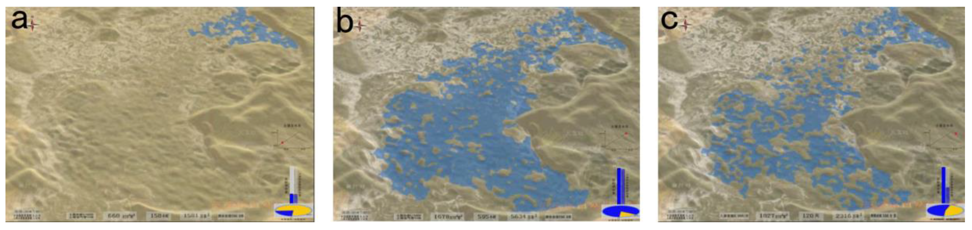
The DLG, DEM and DOM are stacked, generating a three-dimensional static model for the study area. During the simulation, the highest water level obtained by the spatial analysis with no effects on farmland, the main road and the village was 130.5 m. In the three-dimensional dynamic simulation, according to the climate and hydrological conditions of the study area, the water supply flow was 30 m3/s. The water level was mapped from the water at ti time using ArcGIS 9.3, and the nearest low-laying land from the water point was filled. One visualization picture at ti time was performed by the 3Dmax-OpenGL software. Then, the water filled next to the low-laying land at the ti+1 time. The low-laying lands were continually filled with the water variation. The N visualization pictures were shown based on the time (Figure 6).
3.3.2. Correction Effect for Water Supply
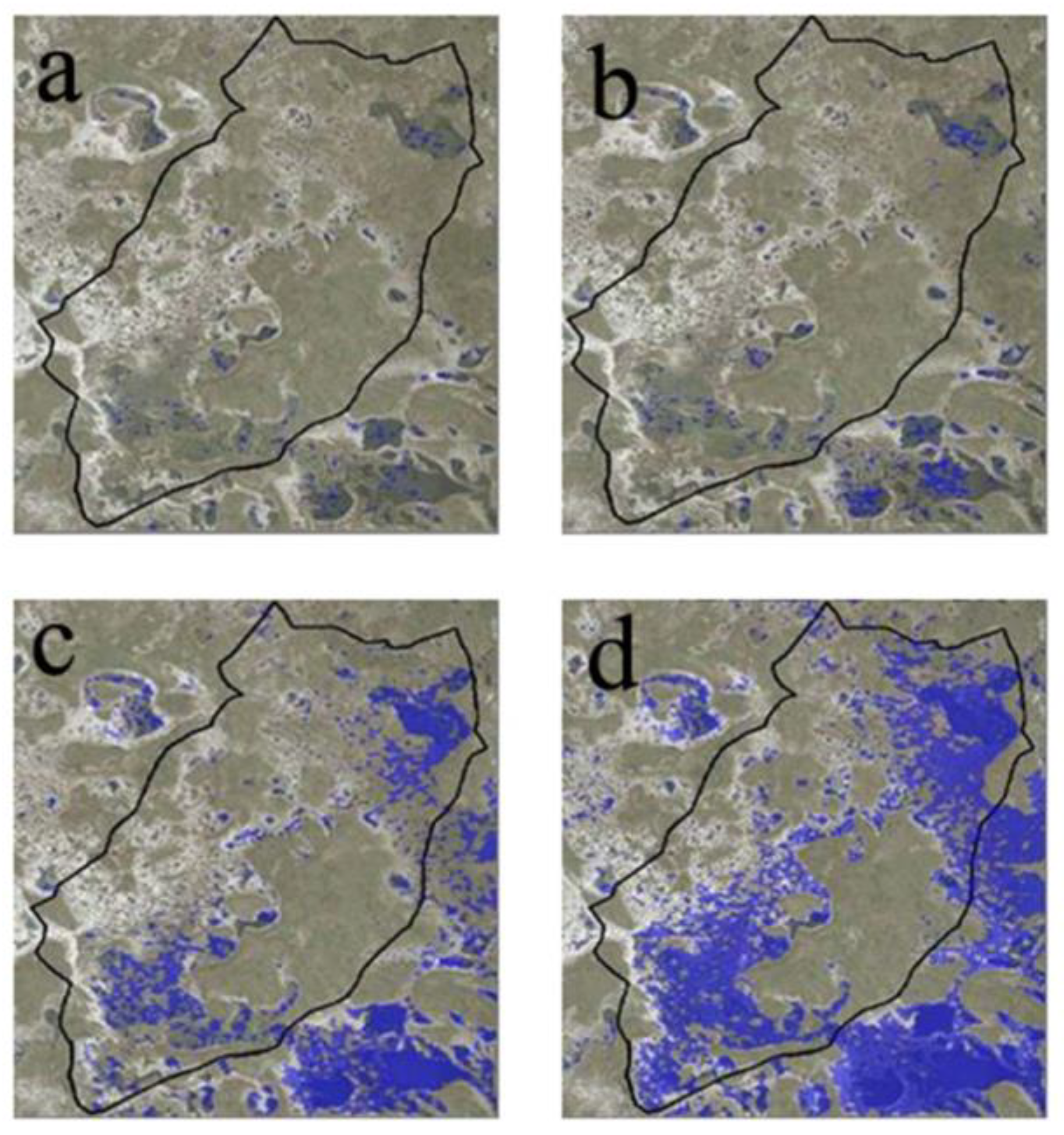
The effect of the water supply in the three-dimensional model can be simulated based on the calculated ecological water demand. Under the condition of a minimum water supply, the simulated β value was 0.83~2.29% (Figure 7a,b), which was less than the expected value (4~7%). Under the condition of an optimum water supply, the simulated β value was 7.98~36.27% (Figure 7c,d), which was less than the expected value (20~70%). These results indicated that there was a difference between the simulated and remote sensed interpreted β values. An examination of the parameters used for calculating the wetland ecological water demand demonstrated that the optimum stopover water level was used to calculate the stopover habitat water demand. However, the water levels were higher than 1 m for some regions in the study area. Therefore, the simulated β value was smaller.
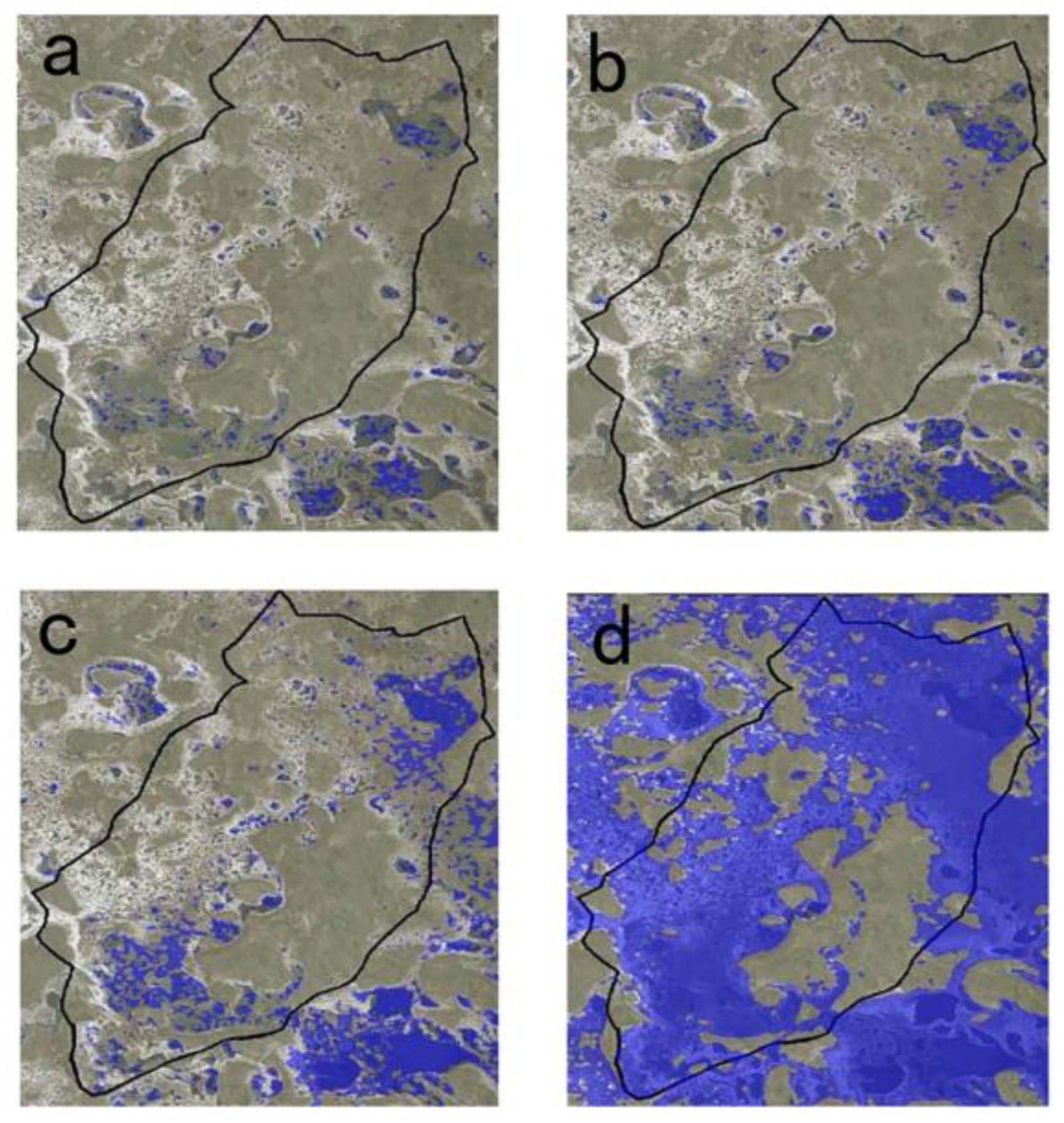
To correct the ecological water demand, the water supply was simulated based on β values of 4%, 7%, 20% and 70%. When the β value is 4~7%, the water area was small and dispersive. Some shallow water meadows appeared in the northeastern region of the study area (Figure 8a). Comparison of the β value of 4%, there are more small water areas with the β value of 7% (Figure 8b). The shallow water wetlands in the northeast of the study area can provide food resources and stopover sites for the Siberian cranes. This result could explain why the Siberian cranes stopped in the northeastern region of the study area when the β value was 4~7%. When the β value was 20%, there were two large water areas in the northeastern and southwestern regions of the study area (Figure 8c), which could provide stopover sites for a large group of Siberian cranes. In addition, some wetlands with small areas and disjunctive distributions in the middle of study area could provide stopover sites for a small number of Siberian cranes. Currently, the area of the study area is approximately 60 km2. When the β value was 70%, the study area was covered by water except hills and farmlands (Figure 8d). As opposed to S. planiculmis, Phragmites australis has become the dominant species. Because of the high-water levels and lack of food, the Siberian crane cannot stop at the study area. A β value of 70% is inadvisable.
Therefore, the ecological water demand of study area can be corrected based on the β value. The minimum β value for Siberian crane stopover sites was 7%, corresponding to the minimum ecological water demand of 3.75 × 10⁸ m3. The optimum β value was 20%, corresponding to the optimum ecological water demand of 5.21 × 10⁸ m3. The simulated minimum ecological water demand was similar to the maximum of the calculated water demand. The simulated optimum ecological water demand was in the range of the calculated optimum water demand. It indicates that these results can provide a reference for wetland restoration and scientific management of the study area.
3.4. Water Resource Management Schemes
A scientific and practical water resource management scheme plays a key role in habitat restoration [32]. The study area is next to the Nenjiang River that has an average annual runoff of 2.15 × 10¹⁰ m3. A water conservation project was conducted by the Chinese government and focused on water diversion from the Nenjiang River for paddy fields and wetland around the study area. The water after irrigating paddy fields enters into wetland. It is an important resource for restoring degraded wetland system. The total annual water diversion is 7.36 × 10⁸ m3. If the water diversion can be reasonably used, then the water supply can meet the optimum ecological water demand with a β value of 20%. Therefore, ecological restoration of the study area is feasible by introducing water from the Nenjiang River.
The water diversion project was influenced by an upstream interception and the hydrological cycle, resulting in a difference between the actual and planned water diversion. An effective water management strategy should be developed to restore the Siberian crane stopover sites. We suggest implementing three schemes to supply water based on different water diversion options.
First, when the water of the Nenjiang River is sufficient and expected water diversion can be reached, continuous water supply is adapted in the thawing period. The water supply refers to the calculated optimum ecological water demand.
Second, water should be provided based on different regions of the study area. In the process of water diversion, if the water supply cannot meet the optimum ecological water demand, then the low-lying land should be restored in the northeastern and southwestern regions of the study area to meet the minimum ecological water demand. This process can provide the improvised stopover sites for the Siberian cranes under conditions of water shortage.
Third, the water supply is provided by a simulated flood. The Nenjiang River, affected by the hydrological periods of wet years and dry years, can provide limited water resources for restoring wetlands in some years. If the water of the study area does not meet the optimum ecological water demand in the implementation process of the water diversion project for 3~5 years, then we should adjust the water diversion from the Nenjiang River and supply water through a simulated flood based on the optimum ecological water demand in the short term. This would keep a hydrological condition of alternating wet and dry. This can limit the growth of xerophytic vegetation in degraded wetlands and provide a basis for wetland restoration.
In different schemes to supply water, the continuous water supply is adapted in the thawing period, but the water supply in different regions and from simulated flood should arrive at an appropriate time. The autumn is defined as the best time to supply water through analysis. There are several reasons for this: (1) in autumn, the agricultural water use needed in the spring is avoided, and water resources can be easily adjusted; (2) the water from Nenjiang River is adequate in the autumn after storing water from rainfall in the summer; (3) the water from paddy fields further increases the available water in the autumn; and (4) the water supply in the autumn can effectively reduce the water shortage the following spring, provide a good habitat for waterfowl, and avoid submerging bird nests.
4. Conclusions
Ecological restoration is an effective way to protect Siberian crane stopover sites. In this study, the minimum and optimum ecological water demand values of 2.47 × 10⁸ m3~3.66 × 10⁸ m3, and 4.96 × 10⁸ m3~10.36 × 10⁸ m3 were calculated, respectively. A three-dimensional model was performed to simulate ecological water demand. However, there is a difference between the calculated and simulated ecological water demands. After correction, the minimum and optimum ecological water demand values suitable for the Siberian crane stopover habitat were 3.75 × 10⁸ m3 and 5.21 × 10⁸ m3, respectively, based on β values of 4%, 7%, 20%, and 70%. In addition, an effective water resource management scheme to protect Siberian crane stopover habitat has been established, including three methods of water supply: continuous water supply when there is sufficient water, water supply only to different regions when there is not sufficient water, and water supply from simulated floods every 3~5 years. The methods to calculate and correct ecological water demand and implement a water resource management scheme in this area can serve as a reference for restoring other waterfowl stopover sites and wetlands in semi-arid areas.
Author Contributions
Methodology, L.S.; software, H.B.; validation, H.J. and C.H.; formal analysis, H.J.; investigation, C.Z.; resource, H.J.; data curation, H.J.; writing—original draft preparation, H.J.; writing—review and editing, H.Y.; visualization, L.W.; supervision, L.S.; project administration, H.J.
Funding
This research was founded by the Special Funds of the State Environmental Protection Public Welfare Industry, grant numbers 201509040; the Fundamental Research Funds for the Central Universities, grant numbers 2412017QD023; and the Foundation of Jilin Educational Committee, grant numbers JJKH20180024KJ.
Conflicts of Interest
The authors declare no conflict of interest.
References
- Debeljak, M.; Džeroski, S.; Jerina, K.; Kobler, A.; Adamič, M. Habitat suitability modelling for red deer (Cervus elaphus L.) in South-central Slovenia with classification trees. Ecol. Model. 2001, 138, 321–330. [Google Scholar] [CrossRef]
- Mitsch, W.J. Wetland creation, restoration, and conservation: A wetland invitational at the Olentangy River Wetland Research Park. Ecol. Eng. 2005, 24, 243–251. [Google Scholar] [CrossRef]
- Bortolotti, L.E.; Vinebrooke, R.D.; St Louis, V.L. Prairie wetland communities recover at different rates following hydrological restoration. Freshw. Biol. 2016, 61, 1874–1890. [Google Scholar] [CrossRef]
- Cooper, D.J.; Kaczynski, K.M.; Sueltenfuss, J.; Gaucherand, S.; Hazen, C. Mountain wetland restoration: The role of hydrologic regime and plant introductions after 15 years in the Colorado Rocky Mountains, USA. Ecol. Eng. 2017, 101, 46–59. [Google Scholar] [CrossRef]
- Cui, B.S.; Yang, Q.C.; Yang, Z.F.; Zhang, K.J. Evaluating the ecological performance of wetland restoration in the Yellow River Delta, China. Ecol. Eng. 2009, 35, 1090–1103. [Google Scholar] [CrossRef]
- Dawson, S.K.; Warton, D.I.; Kingsford, R.T.; Berney, P.; Keith, D.A.; Catford, J.A. Plant traits of propagule banks and standing vegetation reveal flooding alleviates impacts of agriculture on wetland restoration. J. Appl. Ecol. 2017, 54, 1907–1918. [Google Scholar] [CrossRef]
- Liu, X.Y.; Tao, K.Y.; Sun, J.; He, C.Q.; Cui, J.; Chen, X.P. The introduction of woody plants for freshwater wetland restoration alters the archaeal community structure in soil. Land Degrad. Dev. 2017, 28, 1933–1942. [Google Scholar] [CrossRef]
- Baird, A.; Wilby, R.L. Eco-hydrology: Plant and water in terrestrial and aquatic environments. J. Ecol. 1999, 88, 1095–1096. [Google Scholar] [CrossRef]
- Hu, Z.J.; Ge, Z.M.; Ma, Q.; Zhang, Z.T.; Tang, C.D.; Cao, H.B.; Zhang, T.Y.; Li, B.; Zhang, L.Q. Revegetation of a native species in a newly formed tidal marsh under varying hydrological conditions and planting densities in the Yangtze Estuary. Ecol. Eng. 2015, 83, 354–363. [Google Scholar] [CrossRef]
- Obolewski, K.; Glinska-Lewczuk, K.; Jarzab, N.; Burandt, P.; Kobus, S.; Kujawa, R.; Okruszko, T.; Grabowska, M.; Lew, S.; Gozdziejewska, A.; et al. Benthic invertebrates in Floodplain Lakes of a Polish River: Structure and biodiversity analyses in relation to hydrological conditions. Pol. J. Environ. Stud. 2014, 23, 1679–1689. [Google Scholar]
- Zhou, J.; Zheng, L.D.; Pan, X.; Li, W.; Kang, X.M.; Li, J.; Ning, Y.; Zhang, M.X.; Cui, L.J. Hydrological conditions affect the interspecific interaction between two emergent wetland species. Front. Plant Sci. 2018, 8, 2253. [Google Scholar] [CrossRef] [PubMed]
- Brandyk, A.; Majewski, G. Modeling of hydrological conditions for the restoration of Przemkowsko-Przeclawskie Wetlands. Annu. Set Environ. Prot. 2013, 15, 371–392. [Google Scholar]
- Carvalho, D.; Horta, P.; Raposeira, H.; Santos, M.; Luís, A.; Cabral, J.A. How do hydrological and climatic conditions influence the diversity and behavioural trends of water birds in small Mediterranean reservoirs? A community-level modelling approach. Ecol. Model. 2013, 257, 80–87. [Google Scholar] [CrossRef]
- Martinez-Martinez, E.; Nejadhashemi, A.P.; Woznicki, S.A.; Love, B.J. Modeling the hydrological significance of wetland restoration scenarios. J. Environ. Manag. 2014, 133, 121–134. [Google Scholar] [CrossRef] [PubMed]
- Fu, X.F.; He, H.M.; Jiang, X.H.; Yang, S.T.; Wang, G.Q. Natural ecological water demand in the lower Heihe River. Front. Environ. Sci. Eng. China 2008, 2, 63–68. [Google Scholar] [CrossRef]
- Jin, X.; Yan, D.H.; Wang, H.; Zhang, C.; Tang, Y.; Yang, G.Y.; Wang, L.H. Study on integrated calculation of ecological water demand for basin system. Sci. China Technol. Sci. 2011, 54, 2638–2648. [Google Scholar] [CrossRef]
- Yu, F.K.; Huang, X.H.; Liang, Q.B.; Yao, P.; Li, X.Y.; Liao, Z.Y.; Duan, C.Q.; Zhang, G.S.; Shao, H.B. Ecological water demand of regional vegetation: The example of the 2010 severe drought in Southwest China. Plant Biosyst. 2015, 149, 100–110. [Google Scholar] [CrossRef]
- Cai, X.; Rosegrant, M.W. Optional water development strategies for the Yellow River Basin: Balancing agricultural and ecological water demands. Water Resour. Res. 2004, 40, 474–480. [Google Scholar] [CrossRef]
- Yan, D.H.; Wang, G.; Wang, H.; Qin, T.L. Assessing ecological land use and water demand of river systems: A case study in Luanhe River, North China. Hydrol. Earth Syst. Sci. 2012, 16, 2469–2483. [Google Scholar] [CrossRef]
- Berkowitz, J.F.; White, J.R. Linking wetland functional rapid assessment models with quantitative hydrological and biogeochemical measurements across a restoration chronosequence. Soil Sci. Soc. Am. J. 2013, 77, 1442–1451. [Google Scholar] [CrossRef]
- He, C.G.; Ishikawa, T.; Sheng, L.X.; Irie, M. Study on the hydrological conditions for the conservation of the nesting habitat of the Red-crowned Crane in Xianghai Wetlands, China. Hydrol. Process. 2009, 23, 612–622. [Google Scholar] [CrossRef]
- Jiang, H.B.; Wen, Y.; Zou, L.F.; Wang, Z.Q.; He, C.G.; Zou, C.L. The effects of a wetland restoration project on the Siberian Crane (Grus leucogeranus) population and stopover habitat in Momoge National Nature Reserve, China. Ecol. Eng. 2016, 96, 170–177. [Google Scholar] [CrossRef]
- Li, Y.P.; Huang, G.H.; Nie, S.L. Planning water resources management systems using a fuzzy-boundary interval-stochastic programming method. Adv. Water Resour. 2010, 33, 1105–1117. [Google Scholar] [CrossRef]
- Rad, A.M.; Ghahramana, B.; Khalili, D.; Ghahremani, Z.; Ardakani, S.A. Integrated meteorological and hydrological drought model: A management tool for proactive water resources planning of semi-arid regions. Adv. Water Resour. 2017, 107, 336–353. [Google Scholar] [CrossRef]
- Li, F.S.; Wu, J.D.; Harris, J.; Burham, J. Number and distribution of cranes wintering at Poyang Lake, China during 2011–2012. Chin. Birds 2012, 3, 180–190. [Google Scholar] [CrossRef] [Green Version]
- Jiang, H.B.; He, C.G.; Sheng, L.X.; Tang, Z.H.; Wen, Y.; Yan, T.T.; Zou, C.L. Hydrological modelling for Siberian Crane Grus Leucogeranus stopover sites in northeast China. PLoS ONE 2015, 10, e0122687. [Google Scholar] [CrossRef] [PubMed]
- Dong, Z.Y.; Wang, Z.M.; Liu, D.W.; Li, L.; Ren, C.Y.; Tang, X.G.; Jia, M.M.; Liu, C.Y. Assessment of habitat suitability for waterbirds in the West Songnen Plain, China, using remote sensing and GIS. Ecol. Eng. 2013, 55, 94–100. [Google Scholar] [CrossRef]
- Wang, X.Y.; Feng, J.; Zhao, J.M. Effects of crude oil residuals on soil chemical properties in oil sites, Momoge Wetland, China. Environ. Monit. Assess. 2010, 161, 271–280. [Google Scholar] [CrossRef] [PubMed]
- Yang, Z.F.; Cui, B.S.; Liu, J.L.; Wang, X.Q.; Liu, C.M. Theory, Methods and Practices of Ecological Environment Water Demand; Science Press: Beijing, China, 2003. [Google Scholar]
- Yang, Z.F.; Liu, J.L.; Sun, T.; Cui, B.S. Environmental Flows in Basins; Science Press: Beijing, China, 2006. [Google Scholar]
- Ning, Y.; Zhang, Z.X.; Cui, L.J.; Zou, C.L. Adaptive significance of and factors affecting plasticity of biomass allocation and rhizome morphology: A case study of the clonal plant Scirpus planiculmis (cyperaceae). Pol. J. Ecol. 2014, 62, 77–88. [Google Scholar] [CrossRef]
- Arfanuzzaman, M.; Rahman, A.A. Sustainable water demand management in the face of rapid urbanization and ground water depletion for social–ecological resilience building. Glob. Ecol. Conserv. 2017, 10, 9–22. [Google Scholar] [CrossRef]
Figure 1.
Trend of precipitation and temperature in the Momoge National Nature Reserve.

Figure 2.
Location of the study area.

Figure 3.
Stopover numbers of Siberian cranes in spring from 1983 to 2006.

Figure 4.
Variation of wetland area in study area.

Figure 5.
Relationship between Siberian crane number and β value.

Figure 6.
Effect of dynamic simulation for water supplementation. (a) initial stage; (b) drained stage; (c) evaporation completing stage.
Figure 6.
Effect of dynamic simulation for water supplementation. (a) initial stage; (b) drained stage; (c) evaporation completing stage.

Figure 7.
Effect of different levels simulated from ecological water demand. (a) The lowest threshold of minimum water demand; (b) the highest threshold of minimum water demand; (c) the lowest threshold of optimum water demand; and (d) the highest threshold of optimum water demand.
Figure 7.
Effect of different levels simulated from ecological water demand. (a) The lowest threshold of minimum water demand; (b) the highest threshold of minimum water demand; (c) the lowest threshold of optimum water demand; and (d) the highest threshold of optimum water demand.

Figure 8.
Effect drawing of different level simulated from β values. (a) β value is 4%; (b) β value is 7%; (c) β value is 20%; and (d) β value is 70%.
Figure 8.
Effect drawing of different level simulated from β values. (a) β value is 4%; (b) β value is 7%; (c) β value is 20%; and (d) β value is 70%.


Table 1.
Water demand for wetland plants.
| Grade | Cover Degree (%) | Study Area (km2) | Evaporation (mm) | Water Demand (108 m3) |
|---|---|---|---|---|
| Minimum | 30–50 | 303.10 | 1000 | 0.91–1.52 |
| Optimum | 60–80 | 303.10 | 1000~1200 | 1.82–2.91 |
Table 2.
Water demand for evaporation.
| Grade | Evaporation (mm) | Area of Study Area (km2) | β (%) | Water Demand (108 m3) |
|---|---|---|---|---|
| Minimum | 1813.4 | 303.10 | 4~7 | 0.22~0.39 |
| Optimum | 1813.4 | 303.10 | 20~70 | 1.10~3.85 |
Table 3.
Water demand for wetland soil.
| Grade | Field Capacity (%) | Soil Thickness (m) | Soil Area (km2) | Water Demand (108 m3) |
|---|---|---|---|---|
| Minimum | 35~45 | 1.2 | 281.88~290.98 | 1.22~1.52 |
| Optimum | 45~55 | 1.2 | 90.93~248.54 | 0.60~1.31 |
Table 4.
Water demand for stopover habitat.
| Grade | Area of Study Area (km2) | β (%) | Water Level (m) | Water Demand (108 m3) |
|---|---|---|---|---|
| Minimum | 303.10 | 4~7 | 0.10~0.20 | 0.01~0.04 |
| Optimum | 303.10 | 20~70 | 0.30~0.50 | 0.18~1.09 |
Table 5.
Water demand for supplying groundwater.
| Grade | Area of Study Area (km2) | β (%) | Permeability Coefficient (m/d) | Supplement Time (d) | Water Demand (108 m3) |
|---|---|---|---|---|---|
| Minimum | 303.10 | 4~7 | 0.005 | 180 | 0.11~0.19 |
| Optimum | 303.10 | 20~70 | 0.005 | 180 | 0.55~1.91 |
Table 6.
Total water demand in study area.
| Grade | Plant (108 m3) | Surface Evaporation (108 m3) | Stopover Habitat (108 m3) | Soil (108 m3) | Water Supplement (108 m3) | Total Water Demand (108 m3) |
|---|---|---|---|---|---|---|
| Minimum | 0.91~1.52 | 0.22~0.39 | 0.01~0.04 | 1.22~1.52 | 0.11~0.19 | 2.47~3.66 |
| Optimum | 1.82~2.91 | 1.10~3.85 | 0.18~1.09 | 0.60~1.31 | 0.55~1.91 | 4.96~10.36 |
© 2018 by the authors. Licensee MDPI, Basel, Switzerland. This article is an open access article distributed under the terms and conditions of the Creative Commons Attribution (CC BY) license (http://creativecommons.org/licenses/by/4.0/).
Share and Cite
MDPI and ACS Style
Jiang, H.; He, C.; Luo, W.; Yang, H.; Sheng, L.; Bian, H.; Zou, C. Hydrological Restoration and Water Resource Management of Siberian Crane (Grus leucogeranus) Stopover Wetlands. Water 2018, 10, 1714. https://doi.org/10.3390/w10121714
AMA Style
Jiang H, He C, Luo W, Yang H, Sheng L, Bian H, Zou C. Hydrological Restoration and Water Resource Management of Siberian Crane (Grus leucogeranus) Stopover Wetlands. Water. 2018; 10(12):1714. https://doi.org/10.3390/w10121714
Chicago/Turabian StyleJiang, Haibo, Chunguang He, Wenbo Luo, Haijun Yang, Lianxi Sheng, Hongfeng Bian, and Changlin Zou. 2018. "Hydrological Restoration and Water Resource Management of Siberian Crane (Grus leucogeranus) Stopover Wetlands" Water 10, no. 12: 1714. https://doi.org/10.3390/w10121714
Note that from the first issue of 2016, this journal uses article numbers instead of page numbers. See further details here.