Evolution of Velocity Field and Vortex Structure during Run-Down of Solitary Wave over Very Steep Beach

Abstract

An experimental results on the spatio-temporal variation of velocity field and vortex structure, generated from the separated boundary layers on the offshore side of the still-water shoreline, during the run-down process of non-breaking solitary waves over a 1:3 sloping beach are presented. Three waves having the incident wave-height to water-depth ratios (H₀/h₀) of 0.363, 0.263, and 0.171 were generated in a wave flume. Two flow visualization techniques and high-speed particle image velocimetry were employed. The primary topics and new findings are: (1) Mechanism of the incipient flow separation, accompanied by formation of the separated shear layer from the beach surface, is elucidated under the adverse pressure gradient, using the fine data of velocity measurements very close to the sloping boundary. (2) Occurrence of hydraulic jump subsequently followed by development of the tongue-shaped free surface and projecting jet is demonstrated through spatio-temporal variation in the Froude number. It is confirmed by a change in the Froude number from supercritical to subcritical range as the free surface rapidly rises from the onshore to offshore side. (3) A complete evolution of the primary vortex structure (including the core position, vortex size, and velocity distribution passing through the vortex core) is first introduced systematically, together with the illustration of temporal variation in the topological structure. The non-dimensional shoreward distance of the vortex core section decreases with the increase in the non-dimensional time. However, the non-dimensional size height of the primary vortex increases with increasing non-dimensional time. (4) Two universal similarity profiles for both the wall jet flow and the shear layer flow demonstrate independency of the two similarity profiles of the wave-height to water-depth ratio and the beach slope. The similarity profiles indicate the promising collapse of the data from three previous studies for 1:20, 1:10, and 1:5 sloping beaches.

1. Introduction

The solitary wave is characterized as a long wave having very stable motion of propagation over constant water depth nearly without changing the wave height and length (Russell [1]). However, as it travels over a sloping beach, it shoals and/or steepens, deforms continuously before breaking (but does not break for a non-breaking wave), and then subsequently starts to run up shoreward until the maximum run-up height has been reached. After reaching the maximum height along the sloping beach, it begins to run down the slope due to the action of gravity. As the water travels down the slope, the flow depth decreases continuously, making the flow supercritical before meeting the subcritical flow in the deep flow zone with decreasing velocity. It can be anticipated that the steeper the sloping beach, the more prominent the effect of gravity on the retreated flow. In Taiwan, as East and West coastal shorelines have beach slope approximately varying from 1:50 to 1:2 and from 1:1000 to 1:100, respectively, the investigation of solitary waves on sloping beaches receives the upmost importance. This kind of study can be utilized to simulate the run-up and run-down process of the waves as well as the shoreward inundation of a long wave or tsunami-like flow. Its aim is to predict the maximum run-up height, and thus, the inundation area of coastal zone for disaster mitigation.

To the best knowledge of the authors, Hall and Watts [2] were the first to investigate the vertical rises (i.e., the maximum run-up heights) of solitary waves traveling over different impermeable slopes. Approximate linear and nonlinear theories were developed by Synolakis [3] to predict the free surface profile and maximum run-up height of solitary waves traveling over a 1:19.85 (mild plane) beach, along with detailed verifications through a series of laboratory experiments for incident wave-height to water-depth ratios (H₀/h₀) in the range of 0.036 to 0.633. Applying the Lagrangian finite-element Boussinesq wave model, Zelt [4] studied, both numerically and experimentally, the characteristics of free surface profiles in the run-up stage of non-breaking and breaking solitary waves on plane beaches with (from mild to very steep) slopes varying from 1:19.85 to 1:2.75. Grilli et al. [5,6] used a completely nonlinear wave model, based upon the equations of potential flow and a series of wave-flume experiments to elucidate the shoaling and breaking features of solitary waves on different beach slopes that ranged from 1:35.0 to 1:6.5 and from 1:100 to 1:8. In their study, the breaking criterion named “slope parameter” and prediction of breaker type were proposed, along with illustration of empirical equations for calculating the water depth and wave celerity at breaking point. Using the combined results of both numerical simulations and flume tests, Lin et al. [7] presented the free surface profiles and velocity fields during the run-up and run-down phases of a solitary wave propagating over a very steep slope of 1:1.732. On the other hand, for a mild slope of 1:20, only the numerical result was presented. In their study, variations of the free surface and velocity field in hydraulic jump during the run-down phases were briefly illustrated, without addressing the boundary layer effect which in turn results in flow separation from the bottom boundary and vortex formation beneath the separated shear layer. Later, Li and Raichlen [8] experimentally investigated the breaking, impact of plunging jet on the sloping bottom with/without splash-up, and the consequent run-up of solitary waves, with H₀/h₀ ranging from 0.03 to 0.40, over a 1:15 plane beach. Using the particle image velocimetry (PIV) measurement technique, Jensen et al. [9] presented experimental results of velocity field and acceleration during the run-up stage of strongly nonlinear waves, for H₀/h₀ varying from 0.12 to 0.665, propagating on a moderately steep beach having a slope of 1:5.37.

Further, by conducting a series of laboratory experiments in a super-tank (300 m long, 5.0 m wide and 5.2 m deep) with H₀/h₀ in the range of 0.012 to 0.338, Hsiao et al. [10] re-examined the existing empirical formulae for wave breaking criterion, wave height variation and maximum run-up height of solitary waves on a 1:60 plane beach. The feature of the plunging solitary wave propagating over a 1:14 sloping bottom was reported by Sumer et al. [11], along with detailed illustrations of the free surface elevation and bed shear stress using hot-film probe. The mean bed shear stress on the sloping bottom was reported to increase considerably during the run-up and run-down phases. Lo et al. [12] conducted an experimental study in three different wave flumes to investigate the free surface elevation, reflected wave, maximum run-up height, mass and momentum fluxes during the run-up and run-down stages of both single and double solitary waves on four different plane beaches having slopes of 1:20, 1:12, 1:10, and 1:2.47. PIV measuring techniques were used by Pedersen et al. [13] to elucidate the disagreements between experimental and theoretical run-up heights of solitary waves traveling on a beach with a slope of 1:5.67; indicating that the former was prominently smaller than the latter, as predicted by the inviscid theory, and that the discrepancy can be attributable to the losses of onshore mass transport induced by the boundary layer flow.

Recently, Lin et al. [14] employed a high-speed PIV (hereafter named HSPIV, for the framing rate no less than 1000 Hz) with a resolution of 1024 × 1024 pixel to investigate spatial variation of the maximum onshore/offshore velocity in the external flows during the run-up/run-down stage of solitary waves traveling over a 1:10 sloping bottom. To observe, qualitatively, the flow separation and separated shear layer generated from a 1:10 sloping bottom during run-down stage of the solitary wave motion, Lin et al. [15] employed thin-layered fluorescent dye. Further, Lin et al. [16] used HSPIV measurement and the particle trajectory method to present an evolution of a solitary wave propagating over a 1:5 sloping bottom. In this study, the formation of vortex generated from the separated shear layer was observed qualitatively using the visualized images. Detailed elucidation for the evolution of vortex structure and associated velocity fields was, however, not addressed quantitatively. In addition, Hwung et al. [17] used experimental results to propose a new concept in evaluating the relative reduction of the maximum run-up height of a solitary wave (with H₀/h₀ = 0.400) passing through submerged barriers having combination from one to three in numbers (deployed from the toe of a 1:20 sloping beach toward onshore). The relative reduction was defined therein as the ratio of the difference between the maximum run-up height without barrier (R) and the counterpart with barriers (R’) to R, i.e., (R − R’)/R. The experimental results without a barrier, associated with the maximum run-up height as well as an instantaneous velocity field and corresponding visualized image of vortex structure, were presented for the solitary wave (with H₀/h₀ = 0.400) traveling over a 1:20 sloping beach. However, the evolution of vortex structure was not analyzed and elucidated.

Most recently, Skene et al. [18] combined a computational fluid dynamics (CFD) model, based on the two-phase incompressible Navier-Stokes equations, and a mathematical model, consisting of the coupled potential flow and nonlinear shallow water theories, to present the results related to water wave overwash of a step by small steepness, periodic incident waves. The CFD model was identified to describe the flow overturning, formation of vortices, and air entrainment process in the neighborhood of step corner where the overwash took place, and to illustrate breaking process in the bores traveling along the step. Higuera et al. [19] used both experimental methods and numerical model (https://github.com/phicau/olaFlow, a modified edition of the open source code, OpenFOAM^®) to investigate the swash flow dynamics generated by a solitary wave on a 1:3 sloping beach. More emphases were focused on the numerical results of bottom shear stress during the run-up and run-down phases and pressure gradient field around the occurrence of hydraulic jump. However, due to relatively insufficient simulation for the shoreline dynamics, the distinctions between calculated results and experimental data become more prominent as time increases, thus leading to the divergent results during the run-down phase.

Based on a literature survey, the key parameters that dominate the features of free surface elevation and velocity field of solitary wave traveling over a plane beach are the beach slope, S₀, and the incident wave-height to water-depth ratio, H₀/h₀. As reported and further emphasized by Grilli et al. [6], the effect of S₀ is more significant than that of H₀/h₀ for determining variation of free surface elevation (also wave height) evolving on the offshore and onshore sides of breaking point. In addition, according to specified terminologies employed in identifying the relative extent of the inclination of the sloping beach, S₀, a gentle or mild beach was called frequently for S₀ ≤ 1:20 (Synolakis [3]; Grilli et al. [6]; Hsiao et al. [10]; and Hwung et al. [17]); beaches having 1:15 ≤ S₀ ≤ 1:8 are called intermediate sloping beaches (Grilli et al. [6]; Lin and Hwung [20]; and Lin et al. [14]); a moderately steep beach designated for S₀ = 1:5.67 and 1:5.37 (Jensen et al. [9]; and Pedersen et al. [13]); and a very steep beach was named for S₀ ≥ 1:4 (Grilli et al. [6]; Lin et al. [7]; and Higuera et al. [19]).

As indicated by Grilli et al. [6], with more emphasis on the slope effect, the features of free surface elevation and global velocity field during the run-up and run-down phases reported in Hwung et al. [17] for S₀ = 1:20, Lin et al. [15,16] for S₀ = 1:10 and 1:5, and Higuera et al. [19] for S₀ = 1:3 demonstrated were fairly different. At this juncture, it is pertinent to mention that neither the detailed mechanism for the incipient flow separation nor a complete evolution of the vortex structure and associated velocity field during the entire run-down phase has been elucidated in these studies to date.

Accordingly, the unknown or still rudimentary key features for a solitary wave during its run-down process are itemized as: (1) Generation of the incipient flow separation, accompanied by separated shear layer from the beach surface; (2) occurrence of hydraulic jump subsequently followed by development of projecting jet; (3) evolution process of the primary vortex and related topological structure, together with the temporal-spatial variation of the core position and strength (in terms of vorticity) of the primary vortex; and (4) similarity profiles for the velocity distribution right passing through the core of the primary vortex that interacts with the solid sloping boundary and the external stream of the retreated flow.

The present study thus aims to elucidate, in depth, the key features abovementioned during the run-down of a solitary wave traveling on a very steep beach having S₀ = 1:3, using the quantitative HSPIV measurement data and qualitative flow-visualized images.

2. Experiment Set-Ups and Instrumentations

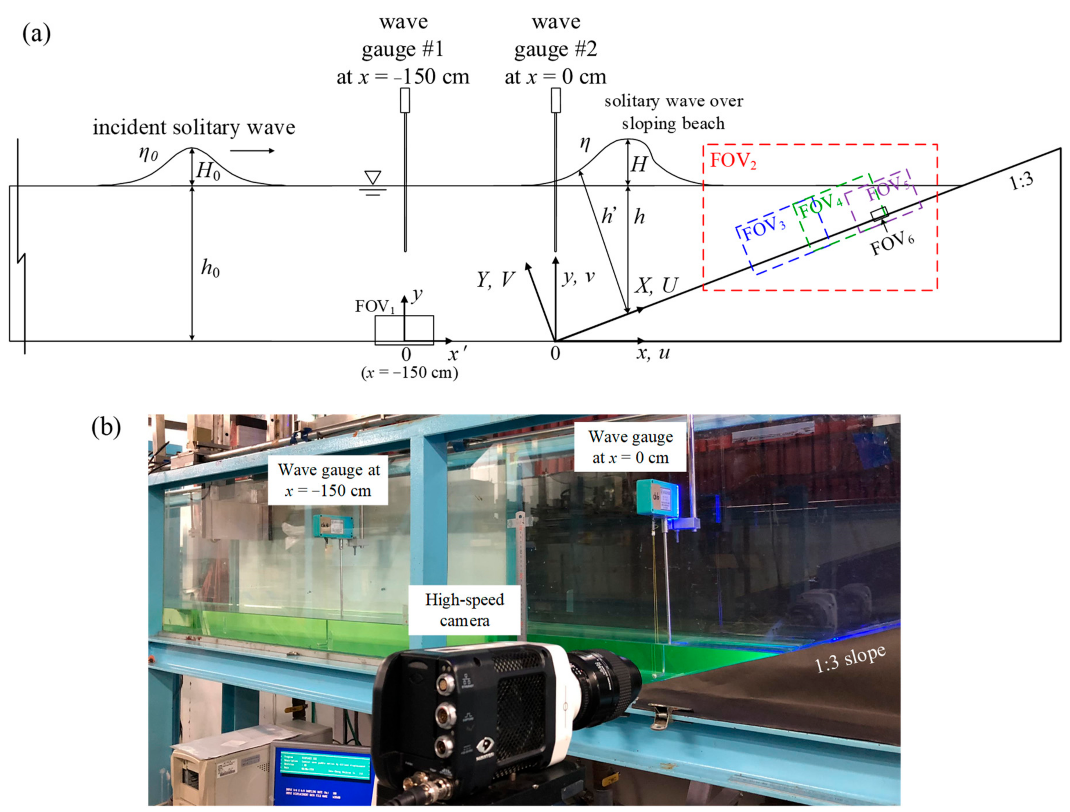
2.1. Wave Flume, Model of Sloping Bottom and Coordinate Systems

Laboratory experiments were conducted in a 14.00 m long, 0.25 m wide, and 0.50 m deep glass-bottomed and glass-walled wave flume. At one end of the flume, a precision servo-motor driven by a piston-type wave maker is mounted, the movement of which could follow the wave-plate trajectory, as presented by Goring [21]. An acrylic sheet of 1.5 cm thick was used to make a 1:3 sloping beach model 200.0 cm long, which was placed with its toe at 900.0 cm from the wave maker (Figure 1a,b).

Two Cartesian coordinate systems were used (see Figure 1a). The first coordinate system has the origin (x, y) = (0, 0) cm located at the toe of the sloping beach with positive x being in the horizontal onshore direction and the positive y in the vertical upward direction. On the other hand, the second coordinate system has the same origin (X, Y) = (x, y) = (0, 0) cm, but with the positive X being oriented shoreward along the sloping beach surface and the positive Y perpendicular upward to the beach surface. The relationship between x and X is x = 0.9487X. The associated velocity components used in the (x, y) and (X, Y) coordinates are (u, v) and (U, V), respectively. Herein, t denotes time and a non-dimensional time is defined as T = t × (g/h₀)^1/2 (with g defined as gravity acceleration), where t = 0 s (also T = 0) characterizes the instant when the crest of the solitary wave is exactly above the toe of the sloping beach, i.e., at x = X = 0 cm.

The free surface elevations and wave heights were measured using two capacitance-type wave gauges, one installed at x = −150.0 cm and the other at x = 0 cm. As shown in Figure 1a, η(x, t) is the instantaneous free surface elevation as well as h(x, t) and h’(X, t) are the still-water depth and the water depth beneath the free surface at the specified positions, x and X, respectively.

2.2. Flow Field Observations Using Flow Visualization Techniques (FVT)

The particle trajectory method was used to determine spatio-temporal variation of the free surface profile, and to visualize the “pathlined” flow structure underneath the free surface. Titanium dioxide (TiO₂) particles having a refractive index of 2.6 and a mean diameter of 1.8 μm were used as seeding particles. The fall velocity (or settling velocity) of titanium dioxide particles, estimated by Stoke’s law, is 4.5 × 10⁻⁴ cm/s. The effect of so tiny value of the falling velocity on the velocity measured can thus be neglected. In addition, the thin-layered fluorescent dye strip was used. The dye was a water solution of both fluorescein sodium (C₂₀H₁₀Na₂O₅) and little salt having a specific gravity of 1.003, measured by a precision hydrometer. The dye strip was injected very slowly and smoothly using a needle onto the beach surface near the still-water shoreline (at x = 24.0 cm) in the spanwise direction as the water mass inside the wave flume remained quiescent. Consequently, a fluorescent dye strip with nearly constant width was formed before the start of wave maker. As a result of solitary wave being generated, the dye strip is then stretched and transported along the sloping beach.

A high-speed digital camera (Phantom M310, Vision Research, see Figure 1b) with a maximum framing rate of 3260 Hz under the largest resolution of 1280 × 800 pixel (with a 12-bit dynamic range) was employed. To visualize the rapid variation in the free surface of solitary wave, the camera was operated at a framing rate of 1000 Hz. On the other hand, to explore the “pathline” pattern of the flow structure as well as the “streakline” pattern of the separated shear layer and the subsequent vortex structures, the sampling rate of this camera was set at 200–500 Hz, depending on the required observation zone. A fan-shaped laser light sheet (of 1.5 mm thickness) was projected upwards through the centerline of glass bottom of the wave flume. The light sheet was used to brighten the two-dimensional motion of uniformly suspended seeding particles on a vertical plane. An argon-ion laser head (Innova-300, Coherent Inc., Santa Clara, CA, USA) with 5 W energy output was used as a light source.

2.3. Velocity Measurements by HSPIV

The HSPIV system is composed of a high speed digital camera, laser head, reflecting mirrors, and optical lens, which were same as those used in FVT. To allow high image resolution and appropriate magnification of the measuring area, a Nikon 200 mm lens (f/4.0D AF Micro-Nikkor) was fitted to the camera. The images of flow fields characterized by the movement of seeding particles (the same as those used in FVT) were continuously recorded using the camera. For easy comprehension, the deployment for the six fields of view FOV₁–FOV₆ over the horizontal bottom and sloping beach is shown schematically in Figure 1a, together with the dimension, range, and pixel resolution of each FOV_i (i = 1–6) being listed in

Table 1. A list of dimension, range, and pixel resolution for each field of view, FOV_i (i = 1–6).

FOVi	Dimension	Range	Pixel Resolution
FOV1	2.00 cm × 1.00 cm	−1.00 cm ≤ x’ ≤ 1.00 cm	1280 × 640
FOV2	9.95 cm × 6.22 cm	10.80 cm ≤ x ≤ 20.08 cm	1280 × 800
FOV3	3.50 cm × 2.19 cm	13.15 cm ≤ X ≤ 16.65 cm	1280 × 800
FOV4	3.50 cm × 2.19 cm	15.75 cm ≤ X ≤ 19.25 cm	1280 × 800
FOV5	2.85 cm × 1.78 cm	17.55 cm ≤ X ≤ 20.40 cm	1280 × 800
FOV6	0.65 cm × 0.41 cm	18.50 cm ≤ X ≤ 19.15 cm	1280 × 800

. To ensure a high time-resolved HSPIV algorithm, a framing rate of 1000/2000/3000 Hz was set while capturing the images of velocity fields with FOV₁/FOV₂/(FOV₃–FOV₆).

Prior to cross-correlation calculation for the velocity field, the instantaneous images captured by HSPIV were processed for contrast enhancement. Firstly, all of the images were treated by Laplacian edge-enhancement technique (Adrian and Westerweel [22]) to intensify the brightness of particles. Secondly, following the image-processing steps used in the hybrid digital particle-tracking velocimetry technique (Cowen and Monismith [23]), the images after contrast enhancement were subtracted from the background images to exclude the constant noise source, if any. The captured images were then processed using cross-correlation technique (MPIV [24] Fortran edition, Mori and Chang [24], and Adrian [25]). The multi-pass PIV algorithm calculated the instantaneous velocity field from a pair of images from the interrogation window size of 64 × 64 pixels with a 50% overlap for the FOV. Both global-range and median filters were used to remove spurious vectors. Consequently missing vectors were interpolated to construct the whole velocity field.

2.4. Experimental Conditions

Three incident solitary waves with H₀/h₀ = 0.363, 0.263 and 0.171 were tested and designated as Cases 1−3, respectively (see

Table 2. A list of experimental conditions.

Case	H0 (cm)	h0 (cm)	H0/h0	Breaker Type
1	2.90	8.0	0.363	Non-breaking
2	2.10	8.0	0.263	Non-breaking
3	2.74	16.0	0.171	Non-breaking

). The solitary waves considered are of a non-breaking type over the sloping beach, which is in good agreement with that identified by the non-dimensional slope parameter (Grilli et al. [6]). Ten repeated runs were performed for the HSPIV measurements for each case. An ensemble-averaged method is used to smooth the velocity time series and to describe the spatial or temporal variation of the velocity fields. Case 1 (H₀/h₀ = 0.363) is used to illustrate a complete evolution (including first run-up, run-down, and second run-up) of the flow field. However, the velocity data of Cases 2 and 3 (H₀/h₀ = 0.263 and 0.171) are employed only in the analysis of similarity profile for the velocity distributions passing through the primary vortex core translating offshore over the sloping beach.

3. Preliminary Tests

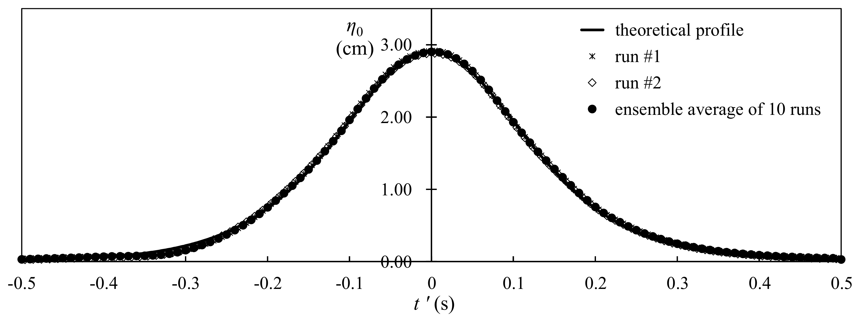
3.1. Verification for Free Surface Elevation over Horizontal Bottom

At first, the free surface elevation of the incident solitary wave, traveling over the horizontal bottom with a constant water depth of h₀, is validated. Figure 2 presents the comparison of the temporal variation in the non-dimensional, 10-run ensemble-averaged free surface elevations η₀(t’)/h₀ for the incident solitary wave of Case 1 measured at the section of x’ (= (x + 150.0) cm) = 0 cm with the theoretical wave profile (Dean and Dalrymple [26]), as given by

$${\eta }_0(x^{\prime },t^{\prime })=H_0{\mathrm{sech}}^2\left[\sqrt{\frac{3H_0}{4{h_0}^3}}(x^{\prime }-C_0{t}^{\prime })\right]$$

(1)

where t’ denotes time and the corresponding non-dimensional time can be defined as T’ = t’ × (g/h₀)^1/2, where t’ = 0 s (also T’ = 0) identifies the instant when the crest of the solitary wave is right above the section of x’ = 0 cm. The (nonlinear) wave celerity C₀ can be obtained theoretically from (g(H₀ + h₀))^1/2 or experimentally from the cross-correlation analysis of the time interval for the wave crest passing the first and second wave gauges (with a separation of 150.0 cm). The experimental results of two individual runs (run #1 and #2) are also plotted in Figure 2 for further comparison. Fairly good agreement between the temporal variation of these three free surface elevations (including run #1 and #2 and 10-run ensemble-averaged data) and that predicted by the theory is clearly observed for Case 1. The results demonstrate the satisfactory generation of incident solitary waves by the wave maker. It should be mentioned that, due to the wave traveling over a constant water depth at the speed of C₀, almost without changing its form (Lin et al. [14,27] and Keulegan [28]), the solitary wave is identified as one of the nearly permanent waves (Mei [29]), but not the dispersive one that disperses into waves of distinct wave periods and lengths (Lin et al. [30]).

3.2. Test for Viscous Effect of Two Sidewalls on Attenuation of Incident Wave Height

To explore the viscous effect of the horizontal glass bottom and two glass sidewalls on the damping/attenuation of incident wave height, the three wave gauges were especially deployed at x = −250.0 cm, −150.0 cm (i.e., x’ = 0 cm), and −50.0 cm (only the free surface elevation measured by the wave gauge at x = −150.0 cm is shown in Figure 2). The measured wave heights at these three sections are H₀ = 2.96, 2.90 and 2.85 cm, respectively, with a still water depth of h₀ = 8.0 cm (Case 1). As reported by Keulegan [28], the following two equations are used to compute the attenuation of wave height for a solitary wave traveling over a horizontal channel of finite width:

[(h₀/H₀)^1/4]_B − [(h₀/H₀)^1/4]_A = K_t × d/h₀

(2)

K_t = K₁ + K₂ = 1/12 × [1 + 2(h₀/W)] × {ν/[g^1/2 × (h₀)^3/2]}^1/2

(3)

here the subscripts “A” and “B” in Equation (2) represent two measuring sections with a separation of d in the wave propagation direction, W is the width of the channel (or the distance between the two sidewalls), and ν is the kinematic viscosity. Note that K₁ (= 1/12 × {ν/(g^1/2 × (h₀)^3/2)}^1/2) is the coefficeint of damping due to bottom friction, and K₂ (= 1/12 × 2(h₀/B) × {ν/(g^1/2 × (h₀)^3/2)}^1/2) represents the coefficient of damping caused by the two sidewalls. Therefore, K_t can be interpreted as the coefficient of combined damping as mentioned. In the present case, the measuring sections A and B are located at x = −250.0 and −50.0 cm, respectively, with h₀ = 8.0 cm, d = 200.0 cm, and W = 25.0 cm. Accordingly, the coefficeints are calculated to be K₁ = 3.13 × 10⁻⁴, K₂ = 1.75 × 10⁻⁴, and K_t = 4.88 × 10⁻⁴, demonstrating that the value of K₂ is smaller than that of K₁ and highlighting that less of a role is played by the friction of two side walls. The relative attenuation of the wave height between x = −250.0 cm and x = −50.0 cm is calculated to be {(H₀)_A − (H₀)_B}/(H₀)_B = 3.7%, in which the influence of two sidewalls is about 1.33% (=3.7% × K₂/K_t). This evidence fairly exhibits the slight effect of the finite width between the two sidewalls on the wave height attenuation and on the value of the incident wave height, H₀.

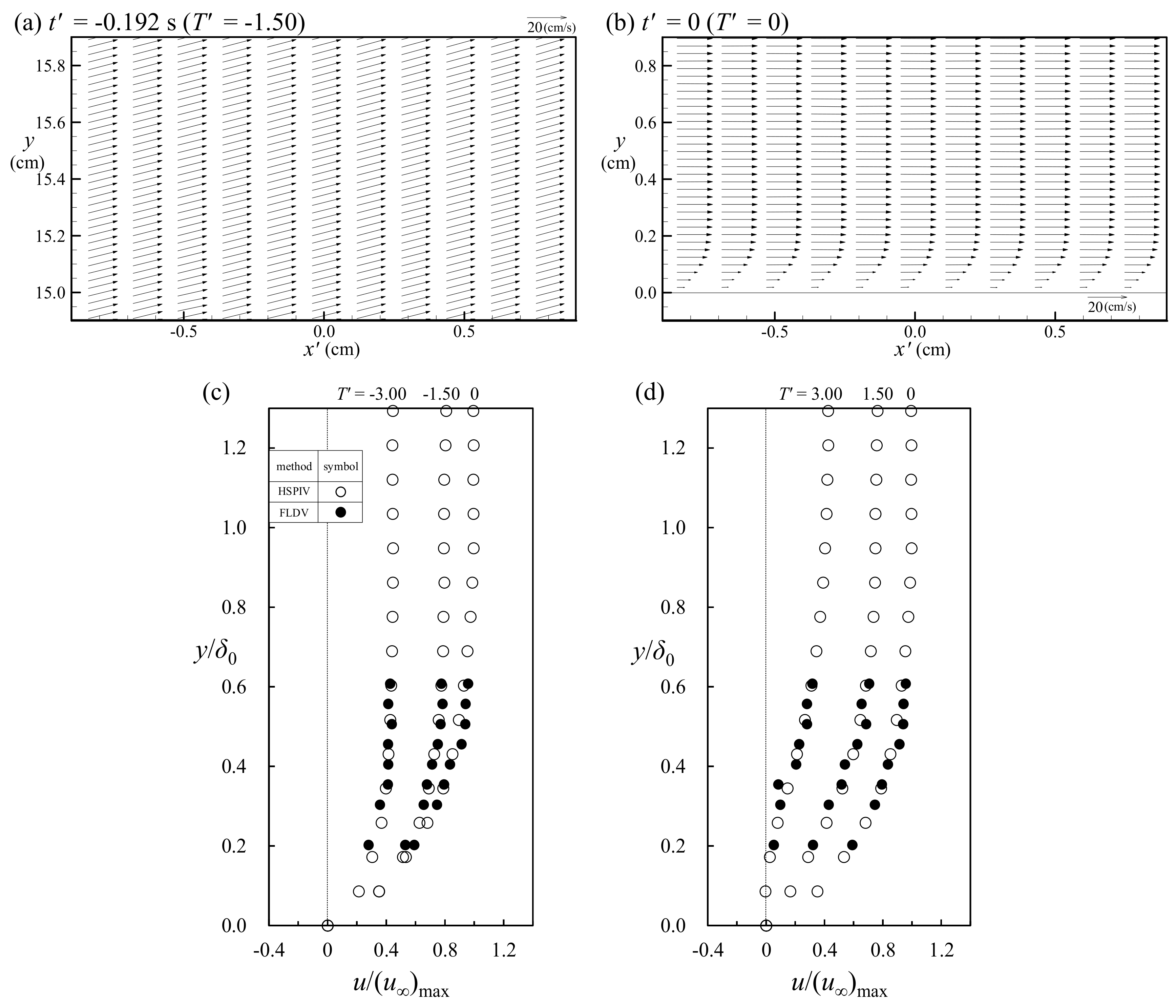
3.3. Verifications for Velocity Fields/Profiles Measured over Horizontal Bottom

Figure 3a,b illustrates two ensemble-averaged velocity fields over the horizontal bottom for 14.90 cm < y < 15.90 cm and 0 cm < y < 0.90 cm, measured around x’ = 0 cm at t’ = −0.135 and 0 s, respectively, for Case 3. Note that the measuring error for identifying the position, y = 0 cm, is about one pixel, equivalent to 0.01563 mm for FOV₁ (with a size of 2.0 cm wide × 1.0 cm high and a resolution of 1280 × 640 pixel). The former/latter represents the velocity field relatively away from/close to the bottom boundary layer before/while the wave crest reaches the section x’ = 0 cm. Following the method proposed by Chang and Liu [31], the measurement error of the velocity is described herein. Assuming the flow is two-dimensional, a continuity check is performed to compute the flux of each grid element F = |∂u/∂x + ∂v/∂y| × dA (in which Δx = Δy = 0.0282 cm for each grid element are used and dA (= Δx × Δy) is the area of a grid element) in the velocity field. Here, a representative flux, F₀ (= (u_∞)_max × Δy) is defined with (u_∞)_max is the free stream velocity outside the bottom boundary layer for t’ = 0 s. The relative error in the flux of the velocity field can be identified as F/F₀. The relative errors F/F₀ at most positions with negligible velocity gradient (see Figure 3a) are less than 2.6%, and the counterparts at locations having significant velocity gradients near the sloping beach (see Figure 3b) are at most 3.2%. These two tiny relative errors identified thus confirm fairly precise measurements in the velocity fields using the HSPIV system.

Figure 3c,d shows comparisons of the temporal variation of the non-dimensional horizontal velocity profiles for Case 3 measured by HSPIV with those obtained using fiber-optic laser Doppler velocimetry (TSI Inc., Shoreview, MN, USA) (Ho [32]) at x’ = 0 cm (i.e., x = −150.0 cm) for −3.00 ≤ T’ ≤ 0 and 0 ≤ T’ ≤ 3.00, respectively. The boundary layer thickness δ₀ and the maximum free stream velocity (u_∞)_max, both taking place at t’ = 0 s (T’ = 0), are used as the representative length and velocity scales, respectively. Herewith, the time-dependent boundary layer thickness, δ(t’), is defined as the distance from the bottom surface to the position where the horizontal velocity u(t’) at the edge of boundary layer is equal to 0.99u_∞(t’) at y’ = δ(t’) (Lin et al. [15,27]; and Sumer et al. [33]). It can be clearly witnessed from Figure 3c,d that the HSPIV data coincide very well with those measured by fiber-optic laser Doppler velocimetry for all of the five time instants, strongly highlighting satisfactory agreements between these two techniques of measurements.

It is worth mentioning that the roughness of the acrylic-made sloping beach surface is typically 7 × 10⁻⁴ cm or smaller [13,34,35], which is several order of magnitudes less than the boundary layer thickness in the present study (about 0.2–0.3 cm, see Figure 3b). Therefore, the beach surface can be treated as smooth and the effect of the roughness of the beach surface on the structure of boundary layer flow can be neglected.

3.4. Identification for Flow Pattern in Boundary Layer over Horizontal Bottom

Following the definitions used in Sumer et al. [33] for solitary wave propagating over constant water depth, the Reynolds number used in the boundary layer flow is defined as R_e = a_m × (u_∞)_max/ν, in which a_m (= (u_∞)_max × t_p/2π) is the amplitude (or half of the stroke) of the water particle displacement in the free-stream region, (u_∞)_max the maximum free stream velocity, and t_p the characteristic time scale that identifies the time width in the time series of either velocity or free surface elevation of solitary wave. In the present Cases 1–3, the corresponding Reynolds numbers R_e being 11,000, 8900 and 13,300 (see Lin et al. [27]) are all much smaller than 2 × 10⁵, indicating laminar flow in the boundary layer (Sumer et al. [33]). It should be mentioned that this study is only applicable to the flow at a laboratory scale. For example, Figure 3c,d has shown fairly identical non-dimensional profiles for different phases with a scale factor of 2.28, implying the existence of the Reynolds-number similitude for the present viscous boundary layer flows. However, scaling these cases to prototype, e.g., by a factor of 100 so that the still water depth is 8.0 m and wave heights of 2.1 and 2.9 m for Cases 1 and 2, would multiply the present R_e by a factor of 1000, thus rendering the values of Reynolds numbers far from the laminar regime and thus into the turbulent regime.

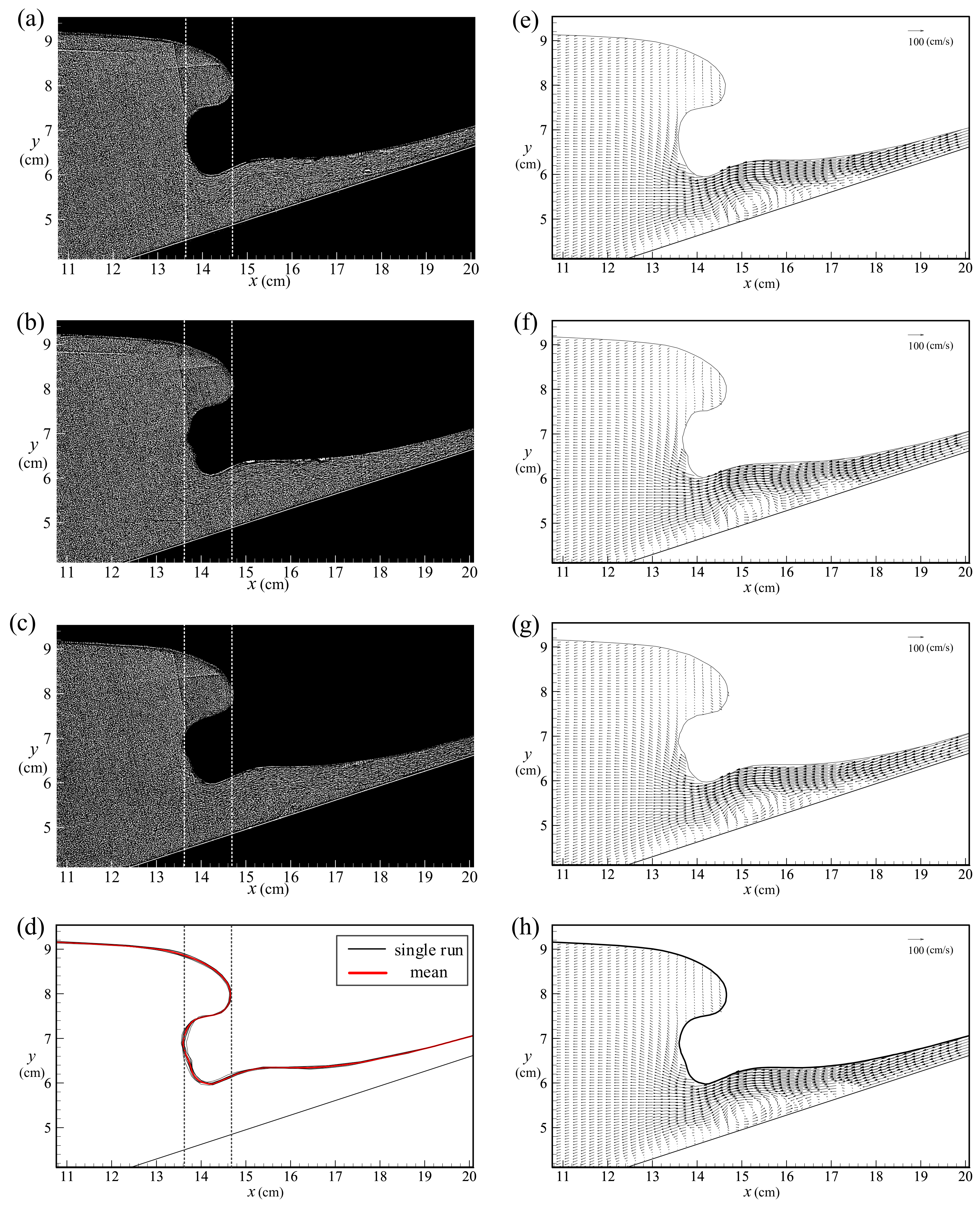
3.5. Repeatability Test for Instantaneous Free Surface Profile and Velocity Field over Sloping Bottom

A repeatability test for the free surface profile of the solitary wave propagating over the 1:3 sloping beach was carried out for Case 1. The high-speed camera was used to capture the instantaneous flow images (see Video attached in Supplementary Material). Figure 4a–c presents three images of the free surface profiles with projecting jet taken at the same time t = 1.048 s (i.e., T = 11.60), but for three different runs randomly selected from 10 repeated ones for 10.76 cm ≤ x ≤ 20.10 cm. It is worth mentioning that the projecting jet shown is not generated by breaking wave, but by hydraulic jump with a “backward” motion (also see Figure 5b). Two vertical dashed lines located at x = 13.60 and 14.68 cm are marked on the images as visual aid for comparison. Note that the tip positions of the three curling tongues are located exactly on the right vertical line, and that the inner-most waist positions beneath these three curling tongues are also nearly situated on the left vertical line. The three observations qualitatively highlight good repeatability for the generated solitary waves over the sloping beach. Figure 4d shows comparison of the ten instantaneous free surface profiles with the ensemble-averaged one obtained from the ten repeated runs. It is seen clearly that the instantaneous free surface profiles have only small difference among distinct runs and agree fairly well with the entire trend of the ensemble-averaged one, demonstrating high repeatability in the free surface profile.

Figure 4e–g shows three instantaneous velocity fields of the projecting jet at the same time, t = 1.048 s, with the free surface profiles of the runs shown in Figure 4a–c, respectively. It is surprisingly found that the three instantaneous velocity fields are not only very similar to each other, but also resemble the ensemble-averaged one (see Figure 4h), confirming good repeatability in the measurements of the instantaneous velocity field. Further, this observation result also implies that the random velocity fluctuations, turbulence, and three-dimensionality are relatively indiscernible and these effects on the velocity field can thus be neglected.

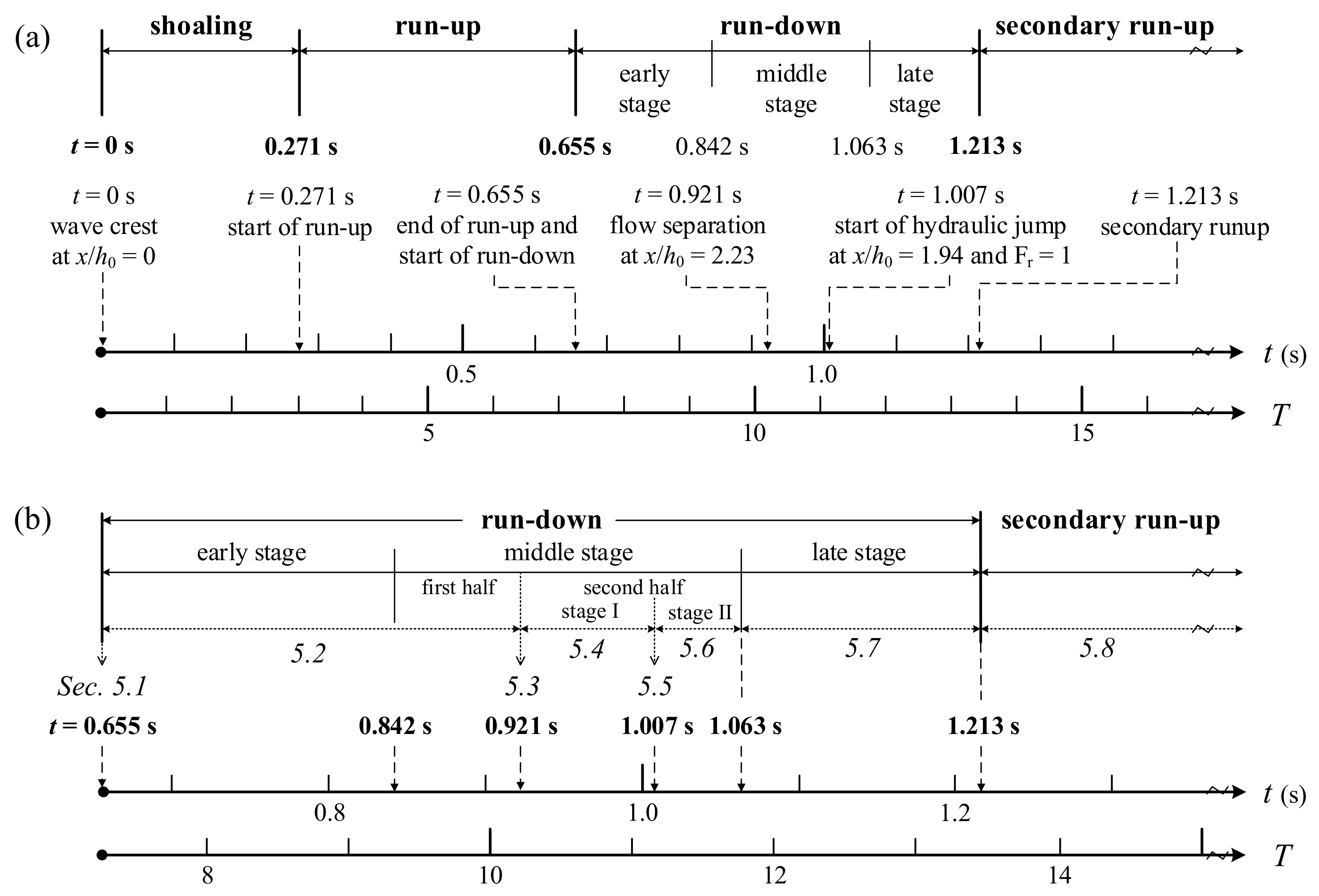
4. General Description of Run-Up and Run-Down Process of Solitary Wave

Following a similar way as stated in Figure 4d, a series of the spatial variations in the ensemble-averaged free surface profile for Case 1 are shown in Figure 5a and are illustrated chronologically as: (1) Wave crest arrives at the toe section (x = 0 cm) of the sloping beach for t = 0 s; (2) wave propagating over the sloping beach accompanied by subsequent initiation of the run-up motion (i.e., without wave breaking) for 0 s < t < 0.655 s; (3) wave motion reaches the maximum run-up height for t = 0.655 s, at which the first run-up motion ends and run-down motion commences; (4) the (first) run-down motion occurs for 0.655 s < t < 1.213 s, during which the incipient flow separation from the beach surface (to be addressed later) and hydraulic jump with sudden rising of the free surface (Sumer et al. [11]) take place for t = 0.921 and 1.007 s, respectively; and (5) the second run-up starts for t ≥ 1.213 s and then continues the motion up to t = 1.351 s.

It should be emphasized that very drastic change of the free surface profile takes place from t = 1.007 s for the occurrence of hydraulic jump, via t = 1.094 s for projecting jet of the curled free surface impinging on the retreated flow, to t = 1.141 s for formation of two-phase turbulent flow. For easy comprehension, a series of the temporal and spatial variations in the free surface profiles are displayed in Figure 5b for 1.007 s ≤ t ≤ 1.141 s. As seen in Figure 5a,b, soon after occurrence of hydraulic jump at t = 1.007 s, the free surface profile of the curling jet takes place at t = 1.017 s and moves “offshore” together with very prominent retreat in the waist portion of the free surface (i.e., positioned at y = 6.4–7.6 cm). For t = 1.048 s, accompanied by successive retreat in the waist portion and continuous decreasing in the water depth at about x > 16.0 cm, the upper free surface and the curling counterpart gets lowered. A comparison of the variation in the curling free surface for t = 1.048 and 1.077 s is made in Figure 5b, exhibiting apparent lowering in the upper and lower portions of the tip-shaped free surface and considerable retreat of the waist portion of the free surface. Due to the action of gravity, the projecting jet keeps bending towards the retreated flow (see Figure 5b for t = 1.085 s) as t increases right before the impingement occurring at t = 1.094 s. Hereafter, the evolution of the primary vortex, with air core being enclosed, can be observed with a two-phase turbulent flow. The other version by using time line to illustrate a complete evolution of solitary wave, including the run-up and run-down processes, is shown schematically in Figure 6a,b for Case 1.

Figure 7a illustrates a close-up of the fluorescent dye strip (with a nearly constant width) equally spanned the central vertical plane over the beach surface, as the water volume inside the wave flume was kept quiescent. Further, Figure 7b–e shows four visualized images associated with the green dye strip being transported on the sloping beach for 0 s ≤ t ≤ 0.921 s, i.e., including the full run-up stage as well as the early and first-half middle stages of run-down for Case 1. The images were captured using a mobile phone camera (iPhone 8 Plus) with a frame rate of 240 Hz, aiming to highlight high color fidelity of the images. The observation was made by the camera viewing the flow field with certain depression angle such that the width of dye strip along the sloping beach can be seen evidently. It is found that a long dye strip partially spans the sloping beach. Due to the onshore and offshore movements of the water particles (very near the beach surface) induced by the solitary wave during the run-up and run-down phases (see Figure 7b–d and Figure 7d,e), the dye strip is transported onshore/offshore almost without changing the width of dye strip. This observation, in fact, demonstrates no discernable motion in the spanwise direction and also the boundary layer flow that is seemingly two-dimensional. Neither a regular array of vortex tubes (with the rotation axis in the spanwise direction) in the laminar flow nor irregular disturbance such as turbulent spot in a transitional flow is observed close to the beach surface. Further, turbulence characterized by the pronounced three-dimensional irregularities as well as high levels of fluctuating velocity and vorticity (Tennekes and Lumley [36]) is not observed at all in the flow. Therefore, the characteristics of the boundary layer in the full run-up and the early run-down stages are in the laminar flow regime, which is lacking in the three-dimensional and turbulent features.

Due to a rapid decrease in the water depth and corresponding increase in flow velocity during the second-half middle stage of run-down, the corresponding field of view, such as that shown in Figure 7b−e, fails to give the flow information underlying the moving free surface in the shallower zone for t > 0.921 s. Instead, the high-speed camera with close-up (viewing normal to the glass sidewall) and the laser light sheet were used to capture the flow field. Under such a situation, the dye strip with a nearly constant width, shown in the visualized images, would exhibit a line appearance right over the beach surface. Figure 7f–j presents five instantaneous streakline patterns (visualized on the vertical plane along the centerline of the wave flume, i.e., 12.5 cm away from the front side wall). These observations reveal the formation of the shear layer separated from the location near x = 17.8 cm (or X = 18.8 cm) at t = 0.921 s, and the subsequent development of the associated vortex patterns for t = 1.007–1.085 s. It is surprisingly found that the vortex structures consisting of very smooth streaklines are clearly seen soon after the incipient flow separation for t > 0.921 s. For examples, at t = 1.007 s for occurrence of hydraulic jump (Figure 5b and Figure 7f), and at t = 1.017–1.077 s for the projecting jet moving downward (Figure 5b and Figure 7g–i). The observed feature still holds true before the projecting jet impinging upon the retreated flow at t = 1.085 s (Figure 5b and Figure 7j). Note that, on the offshore and onshore sides of these streaklined shear layer and vortex structure, the dye strip with nearly constant width is still observed evidently without exhibiting prominent three-dimensional or turbulent flow features. These observations for t ≤ 1.094 s indicate the two-dimensional feature of the boundary layer induced by the non-breaking solitary wave propagating over the 1:3 sloping beach. However, two-phase turbulent flow occurs for t > 1.094 s because the projecting jet have impinged upon the retreated flow with air bubbles being entrained into the flow.

Similarly, Figure 7k–o presents five streaklined flow fields each with the same time as that shown in Figure 7f–j, respectively, but visualized on the vertical plane 8.0 cm away from the front sidewall. Note that the streakline patterns shown in the middle and right columns of Figure 7, at any one of the five time instants, are fairly identical, strongly demonstrating the boundary layer flow is nearly two-dimensional, lacking in obvious three-dimensional or turbulent flow characteristics. Therefore, the following section addresses only the characteristics of the two-dimensional flow field.

5. Results and Discussion for Complete Evolution of Run-Down (Case 1)

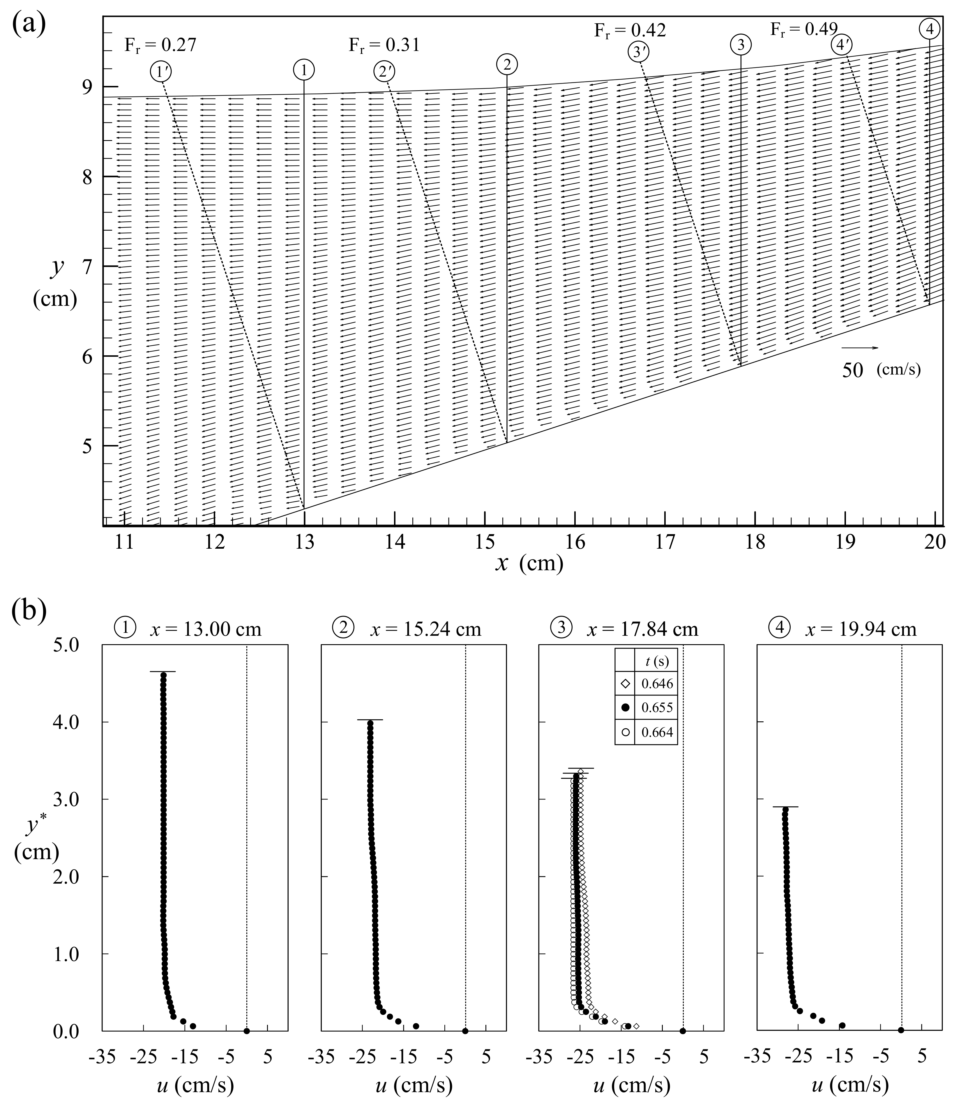
5.1. Start of Run-Down at t = 0.655 s

Figure 8a presents the spatial variation in the ensemble-averaged velocity field for 10.8 cm ≤ x ≤ 20.1 cm (11.38 cm ≤ X ≤ 21.19 cm) at t = 0.655 s for Case 1, specifying the end of run-up phase at which wave motion has reached the maximum run-up height and the start of run-down phase. It is found that all of the horizontal velocities have taken negative values, indicating the onset of run-down phase at this moment when the free surface of the wave exactly reaches its maximum onshore position. This evidence strongly exhibits prominent phase-lead of the offshore velocity field over the onshore propagation of the wave free surface. Figure 8b shows the profiles of u(y*), obtained at four different shoreward distances x (= 0.9487X) for t = 0.655 s, as illustrated in Figure 8a, with four vertical lines each having a circled number (from ① to ④), and y* = y − x/3. It is found that, at the most shoreward distance of x = 19.94 cm (X = 21.02 cm), the u(y*) profile exhibits quasi-linear distribution approximately, except that in the bottom boundary layer (Lin et al. [15,27]). However, as the shoreward distance decreases, the distribution of u(y*) is more toward uniform (but excludes that close to the bottom). Herein, the horizontal uniform or partially-depth-averaged velocity, u_u(x, t), is defined as the mean of velocities only within uniform or quasi-linear part of the whole distribution, i.e., without taking the velocities inside boundary layer flow into account. Note that the spatial and temporal variations of u_u(x, t) can be used as an indicator of flow acceleration or deceleration.

As shown in Figure 8b, the magnitude of the (offshore) uniform velocity u_u(x, t) existing within each velocity profile is observed to decrease continuously from 27.5 cm/s to 20.1 cm/s with decreasing shoreward distance from x = 19.94 cm (X = 21.02 cm) to x = 13.00 cm (X = 13.70 cm), respectively. These values of u_u(x, t) indicate the retreated flow decelerated spatially in the offshore direction for t = 0.655 s due to the convective acceleration (Daily and Harleman [37]) positive/negative in the onshore/offshore direction. More interestingly, as observed from the sub-figure ③ of Figure 8b for x = 17.84 cm (X = 18.80 cm), the magnitude of u_u increases with increasing t for t = 0.646–0.664 s. This observation strongly reveals that the retreated flow is temporally accelerated in the offshore direction because the local acceleration (Daily and Harleman [37]) holds positive/negative value in the offshore/onshore direction.

Following the approach adopted by Henderson [38], Chow [39], and Subramanya [40], the velocity component in parallel to and the water depth normal to the sloping bottom should be used to compute the Froude number for a flow moving over a sloping boundary. Accordingly, the Froude number is defined as F_r = −U_d/(gh’)^1/2 where U_d(X, t) is the depth-averaged velocity of U(X, Y, t) along the Y axis. Figure 8a also shows the corresponding Froude number at each section of the four inclined lines (marked with the numbers from 1’ to 4’ in a circle). The Froude numbers decrease continuously from F_r = 0.49 at x = 19.94 cm (i.e., X = 21.02 cm) to F_r = 0.27 at x = 13.00 cm (i.e., X = 13.70 cm) and are all smaller than unity, demonstrating that the retreated flow is subcritical at t = 0.655 s (i.e., the moment for the start of run-down).

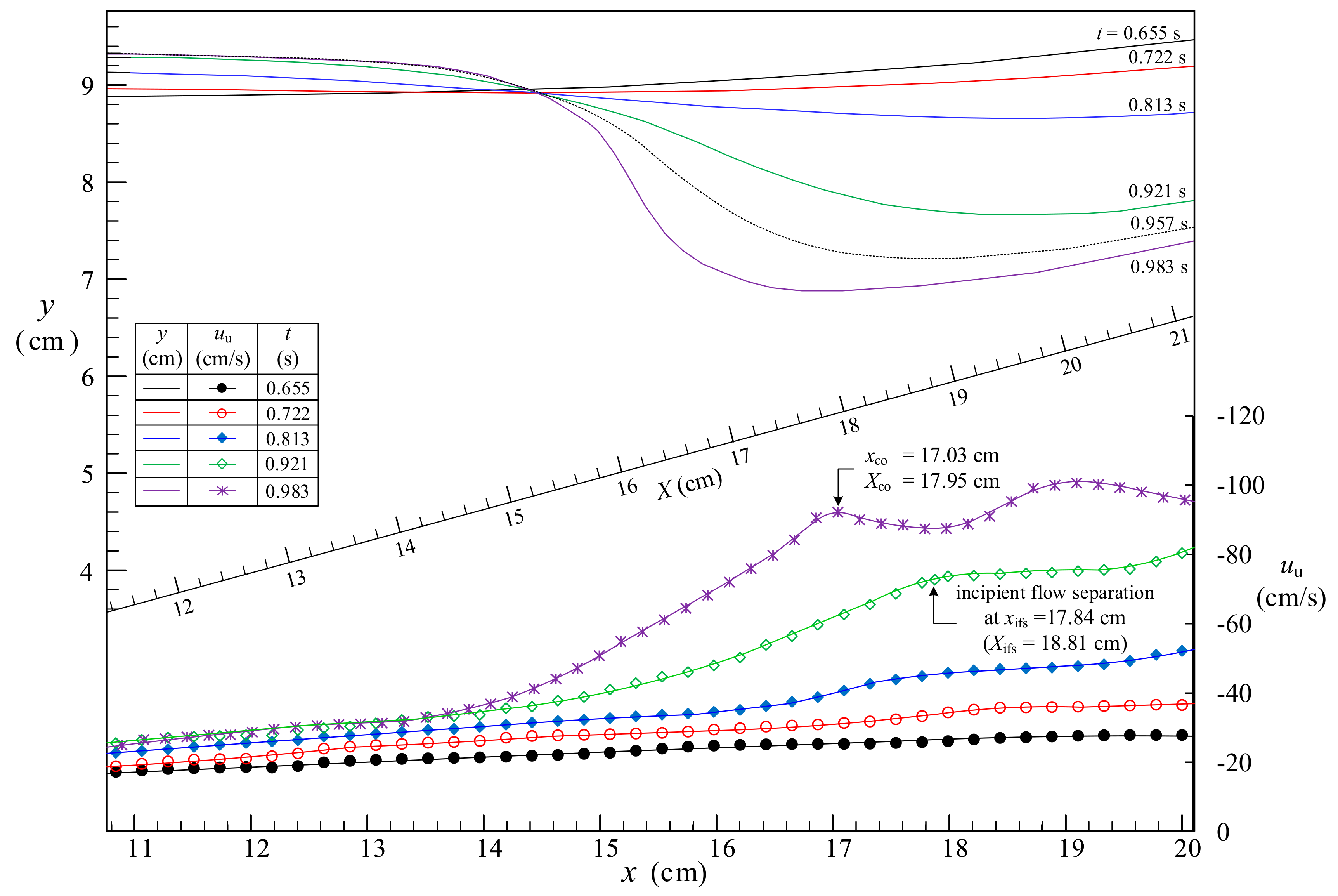
5.2. Early and First-Half Middle Stages of Run-Down for 0.655 s < t < 0.921 s

Once the maximum run-up height has been reached at t = 0.655 s, the water in the shallower region over the sloping beach is then driven by gravity, thus leading to a retreated flow generated for t > 0.655 s, and then undergoes run-down motion. Figure 9 shows a summarized plot for the spatial variation of the (offshore) horizontal uniform velocity u_u(x, t), along with the spatial change of free surface profile for 0.655 s ≤ t ≤ 0.983 s (Case 1), exhibiting successive depression of the free surface elevations in the region for x > 14.6 cm (i.e., X > 15.39 cm). Further, for t = 0.722/0.813 s, prominent decrease in the magnitude of u_u(x, t) in the offshore direction occurs from 36.6/52.5 cm/s at x = 20.1 cm (X = 21.19 cm) to 27.8/31.9 cm/s at x = 14.6 cm (X = 15.39 cm), respectively. This observation clearly indicates that the retreated flow is decelerated spatially in the offshore direction. More interestingly, the magnitude of u_u increases with increasing t for t = 0.655–0.921 s at any specified shoreward distance between x = 10.8 cm (X = 11.38 cm) and x = 20.1 cm (X = 21.19 cm) (see Figure 9), which strongly reveals that the retreated flow is accelerated temporally in the offshore direction.

As seen in Figure 10 for t = 0.813 s, the Froude number decreases successively from F_r = 1.15 at X = 21.02 cm, via F_r = 0.75 at X = 18.81 cm, to F_r = 0.46 at X = 16.06 cm. The result demonstrates the change in the retreated flow condition from supercritical state (F_r > 1.0) on the onshore side to a sub-critical one (F_r < 1.0) on the offshore side. The critical section (F_r = 1.0) occurs is located at X = X_cr = 20.32 cm (not shown). Soon after t > 0.813 s, the water depth still keeps decreasing for X > 15.39 cm (i.e., x > 14.6 cm, see Figure 9). At the same time, the retreated flow remains decelerated spatially and accelerated temporally in the offshore direction due to the effect of gravity. As a result, a supercritical flow is formed and moves offshore toward the deeper region where a subcritical flow exists. Therefore, a critical flow should exist between the deeper and shallower regions.

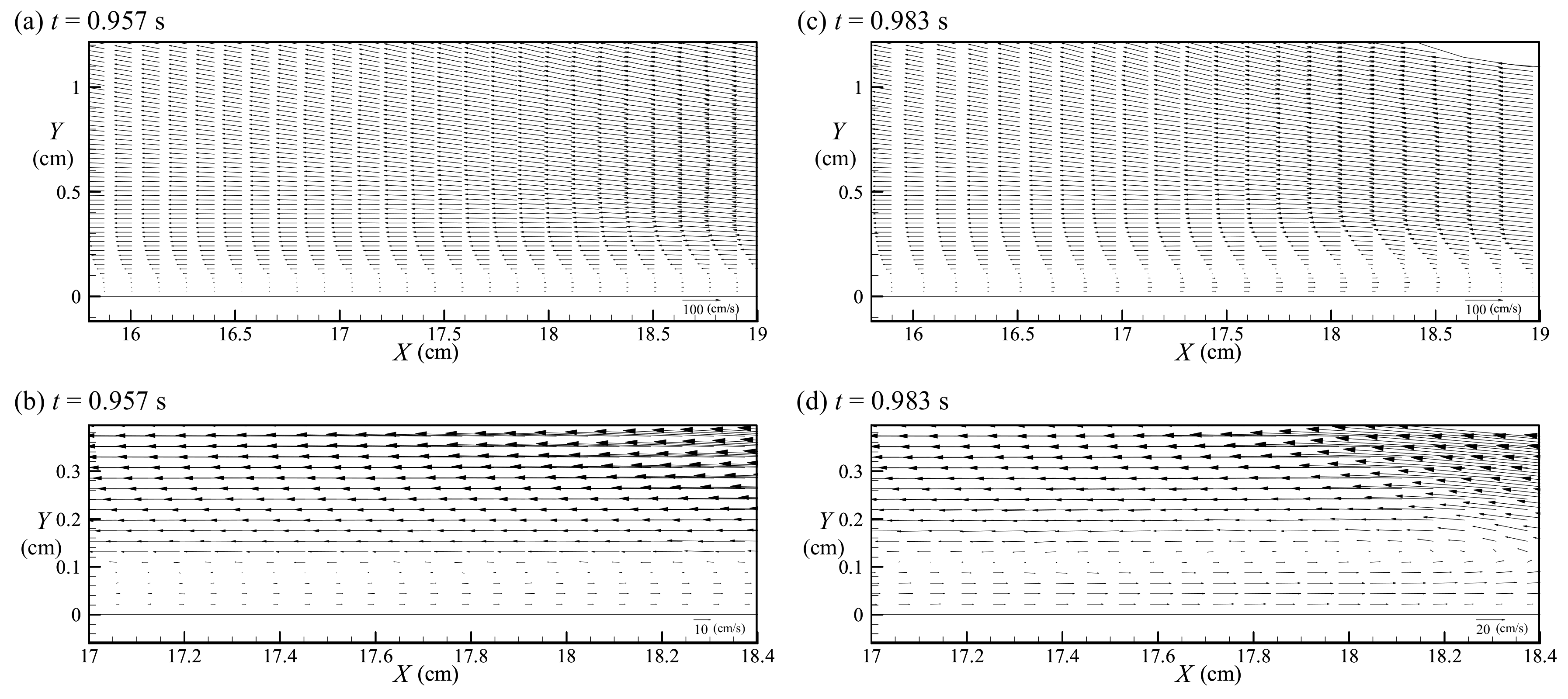
5.3. Incipient Flow Separation from Beach Surface at t = 0.921 s

Figure 11a illustrates the spatial variations of the velocity field and free surface profile having a very streamlined pattern between x = 14.6 cm (X = 15.39 cm) and x = 20.1 cm (X = 21.19 cm) at t = 0.921 s for Case 1. The corresponding variations of the free surface profile and the horizontal uniform velocity with the shoreward distance for t = 0.921 s can also be seen in Figure 9, in which very prominent depression of the free surface elevation takes place for 14.6 cm ≤ x ≤ 20.1 cm (15.39 cm ≤ X ≤ 21.19 cm). Note that, for t = 0.921 s, more profound decrease in the magnitude of the (offshore) horizontal uniform velocity u_u(x) changing from 81.5 cm/s at x = 20.1 cm (X = 21.19 cm) to 25.5 cm/s at x = 10.8 cm (X = 11.38 cm) strongly implies spatial deceleration of the retreated flow and adverse pressure gradient in the offshore direction. Further, as is also seen in Figure 11a, the Froude numbers marked near the circle numbers ①–⑤ indicate that the smaller/greater the water depth, the greater/smaller the Froude number. It is pertinent to mention that the critical flow appears at the section, X = X_cr = 18.04 cm (not shown) for t = 0.921 s, which is more offshore than that for t = 0.813 s (i.e., at X_cr = 20.32 cm).

Figure 11b,c presents a near-bottom velocity field and three velocity profiles measured in the boundary layer at three different locations for t = 0.921 s, respectively. In addition, Figure 11d illustrates a close-up and summarized edition for displaying the data that is very close to the sloping beach for the three velocity profiles shown in Figure 11c. The incipient flow separation (Schlichting [41]) does occur at X = X_ifs = 18.81 cm (see sub-figure 2’ of Figure 11c), which is located on the onshore side of the critical section (X_cr = 18.04 cm) with supercritical flow (see Figure 11a). As, very close to the beach surface, the gradient of the velocity component U(Y) with respect to Y is first identified to be zero; and because, on the offshore and onshore sides of the incipient flow separation point, the velocities very close to the sloping beach take the positive and negative values for Y < 0.023 cm (Figure 11d), respectively. Soon after the incipient flow separation at t = 0.921 s, the fluid particles that are very close to the beach surface move away and transport toward the external stream of retreated flow, and then to displace in a direction opposite to the external stream, resulting in a very thin recirculation zone under the separated shear layer. It is worth mentioning that the instant for the critical flow taking place right at the section of incipient flow separation (i.e., the critical section at X_cr = X_ifs = 18.81 cm) is corresponding to t = 0.874 s (not shown).

5.4. Second-Half Middle Stage I of Run-Down for 0.921 s < t < 1.007 s

Figure 12a,b illustrates the near-bottom velocity field and the corresponding close-up right over the beach surface, in which an elongated recirculation zone with onshore velocities very close to the sloping bottom can be identified near X = 17.0–19.0 cm at t = 0.957 s. This zone highlights the formation of primary vortex in the early stage of its entire evolution under the separated shear layer. Further, pronounced onshore velocities appear very near the sloping beach for Y < (0.07–0.085) cm, zero velocity takes place at about Y = (0.07–0.085) cm, and offshore velocities appear approximately for Y > (0.07–0.085) cm, respectively. Due to energy supply extracted from the supercritical retreated flow into the recirculation zone via momentum transfer by the separated shear layer, the primary vortex consequently develops with its size becoming larger and its core position moving more offshore with increase in t.

Figure 12c,d shows the counterparts of Figure 12a,b measured at t = 0.983 s to confirm the spatial deceleration of the retreated flow and the developing process of primary vortex under the separated shear layer. The (offshore) uniform velocity at any specified section in Figure 12c is larger than that in Figure 12a, revealing the temporal acceleration of the retreated flow. As seen in Figure 12d, the magnitudes and thicknesses of the onshore velocity zone occurring below the vortex core are greater than those at t = 0.957 s (see Figure 12b). Using the streamline pattern corresponding to Figure 12d (not shown), the size of the primary vortex can be defined as the height measured from the sloping beach, through the vortex core and along the positive Y direction, then up to a specified point. At this point, the most outside streamline surrounding the primary vortex is nearly confluent with, but parallel to the instantaneous one that stems from either the flow separation point or the saddle point (Lin et al. [42]). Such a height is termed hereafter “size height” and denoted by Y_size. For t = 0.983 s, the size height can be estimated to be Y_size = 0.21 cm at the section where the primary vortex core is located (hereafter named “core section” and defined as X_co), i.e., X = X_co = 17.95 cm.

It is worth mentioning that, for t = 0.957 and 0.983 s, the critical sections appear at X_cr = 17.44 and 17.08 cm, respectively, which are located at more offshore positions than that (=18.04 cm) for t = 0.921 s. Further, as is also seen in Figure 8, the nature of the horizontal uniform velocity u_u for t = 0.983 s is very different from those for t = 0.813 and 0.921 s. It does highlight the decrease of |u_u| from x = 19.0 cm (X = 20.03 cm) down to a local minimum (=87.3 cm/s) at about x = 17.9 cm (X = 18.87 cm), then an increase of |u_u| up to a local maximum (=92.3 cm/s) at x = 17.03 cm (X = 17.95 cm), and finally a prominent decrease of |u_u| down to the value of 36.3 cm/s at about x = 14.0 cm (X = 14.76 cm). Such a variation feature can be attributable to the influence of the rotational and translating motion of the primary vortex (with its core at x_co = 17.03 cm or X_co = 17.95 cm), as evidenced in Figure 12c,d.

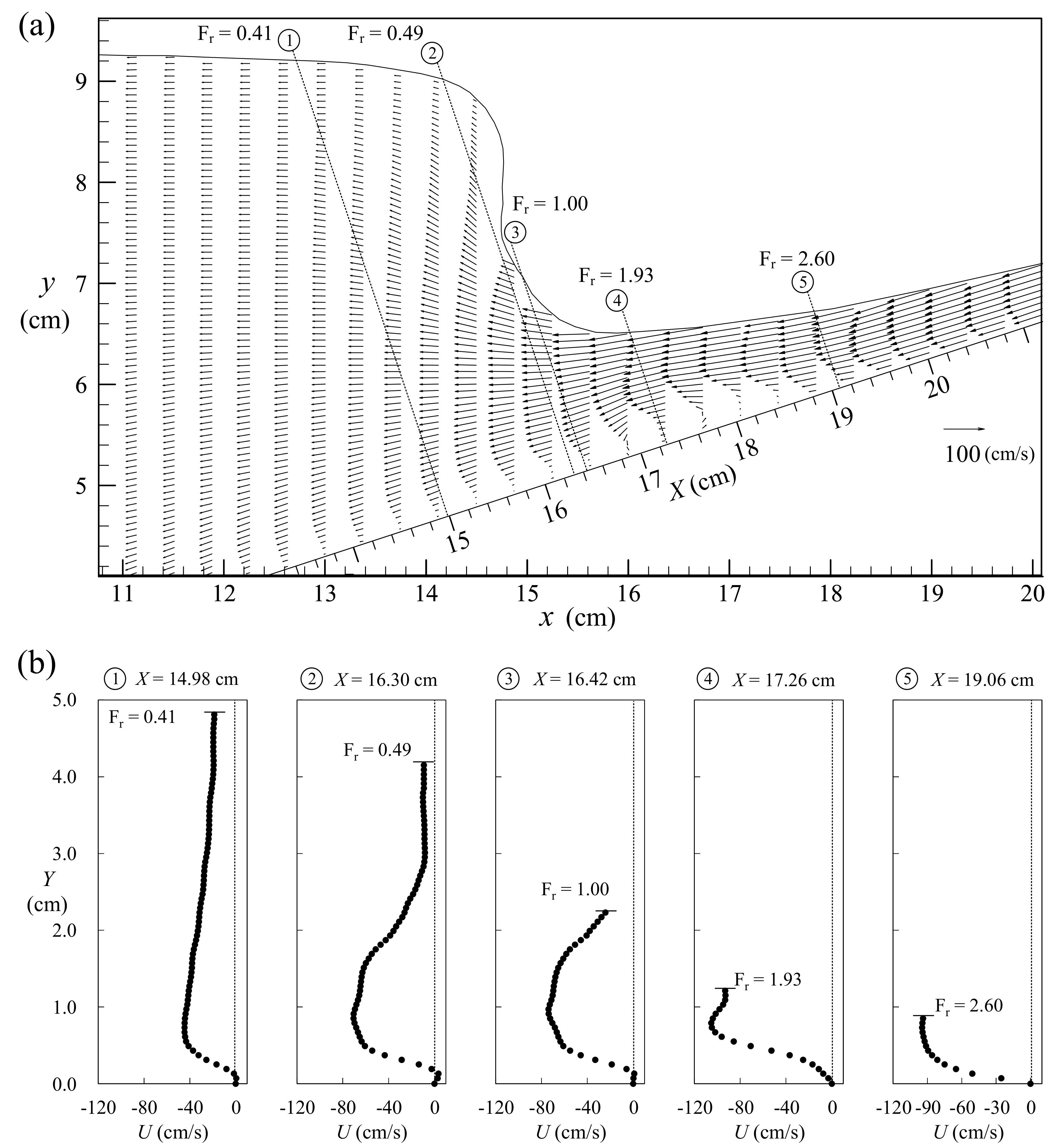
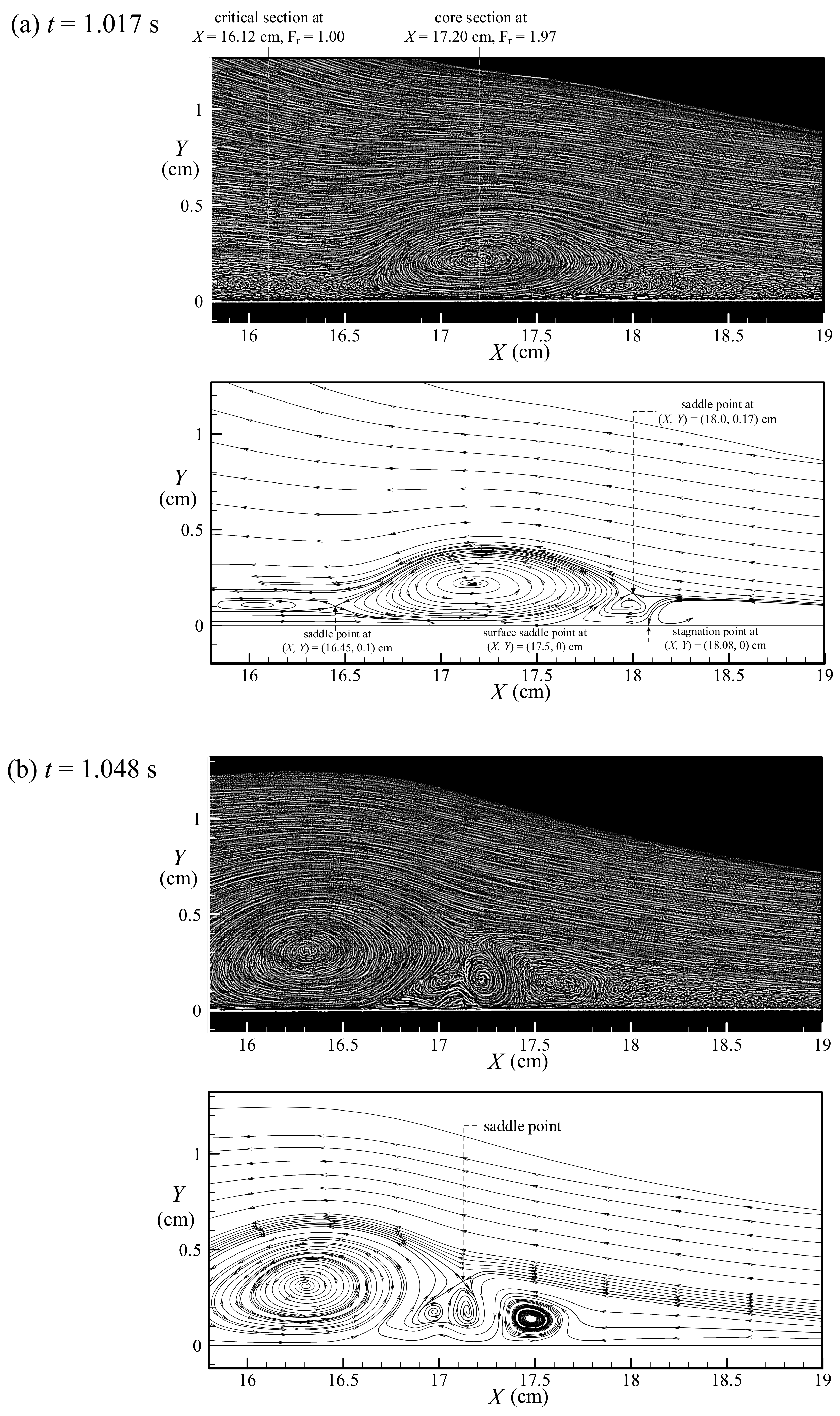
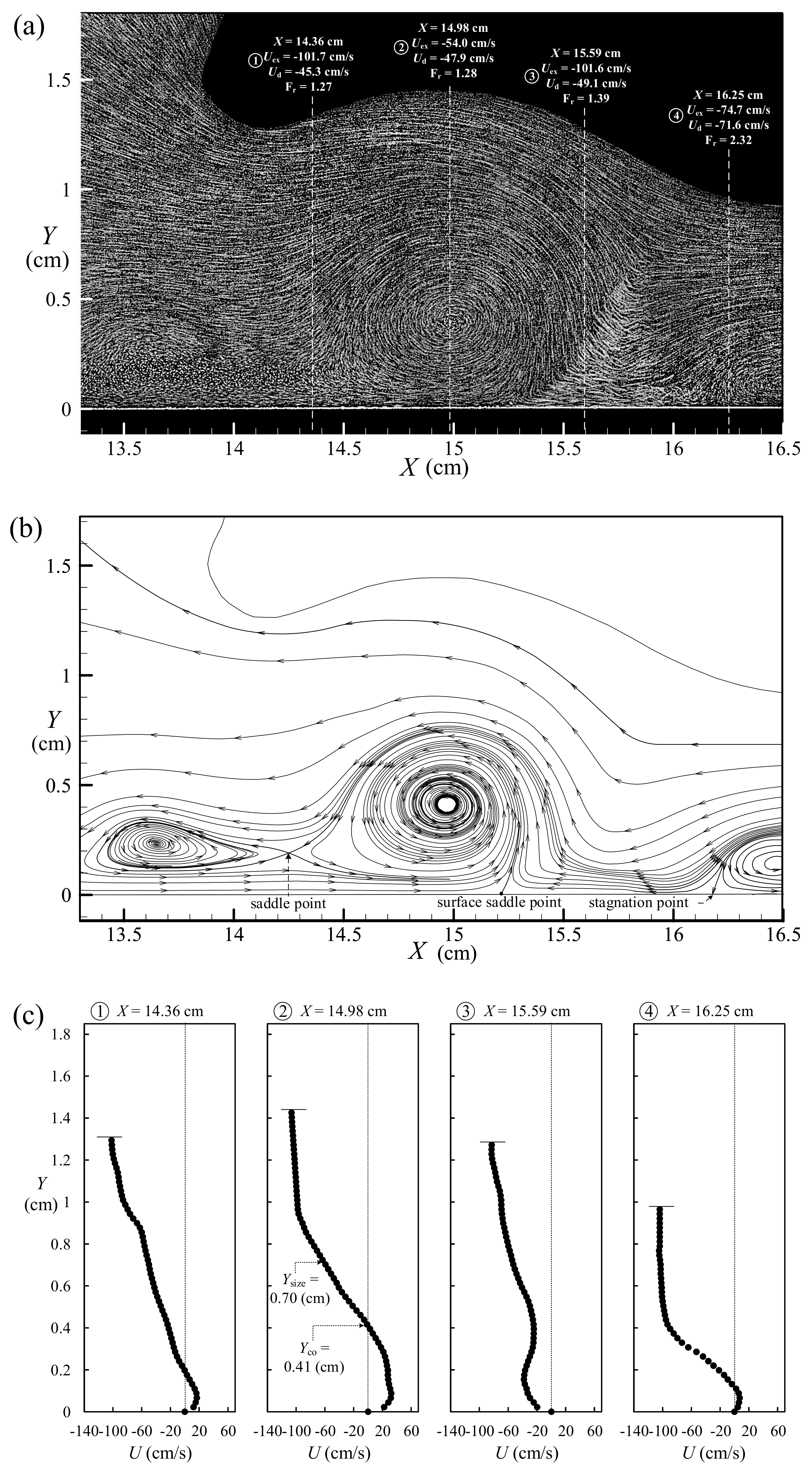
5.5. Incipient Hydraulic Jump at t = 1.007 s

As seen in Figure 8 for t = 0.983 s, more drastic lowering of the free surface is observed and is soon followed by the abrupt rising of the free surface profile. Figure 13a presents the ensemble-averaged velocity field obtained at t = 1.007 s for 10.8 cm ≤ x ≤ 20.1 cm, over which a sudden rise of free surface is seen around x = 14.4–15.2 cm. This feature marks the beginning of hydraulic jump (Sumer et al. [11]). Further, Figure 13b shows five velocity profiles of U(Y) for time t = 1.007 s, each labeled with the measuring section-number and position, together with the values of the Froude number. It is seen that the Froude number in the shallower/deeper water depth is larger/smaller than unity, indicating occurrence of the supercritical/subcritical flow. Note that the critical section is located at X_cr = 16.42 cm, see section ③ in Figure 13b.

The visualized image at t = 1.007 s, shown in Figure 14a, illustrates the well-organized primary vortex structure (accompanied by the two smaller vortices located on both sides of the primary vortex) developing with the core centering at X_co = 17.41 cm. Figure 14b presents the instantaneous streamline pattern (obtained from the corresponding velocity field), indicating the size height and core section of the primary vortex are, respectively, equal to Y_size = 0.36 cm and X_co = 17.41 cm, which are in good agreement with those observed from visualized image (see Figure 14a). With reference to the retreated flow, the velocity profile measured at X_co =17.41 cm exhibits the “opposite (i.e., onshore) flow” distributing from the bottom surface up to the core height. Further, the Froude number at X_co = 17.41 cm is still larger than unity (with F_r = 1.97), identifying the retreated flow at the core section is supercritical. It should be mentioned that, for t = 1.007 s, the critical flow occurs at X_cr = 16.42 cm (Figure 13a), which is located on the offshore side of the core section (at X_co = 17.41 cm).

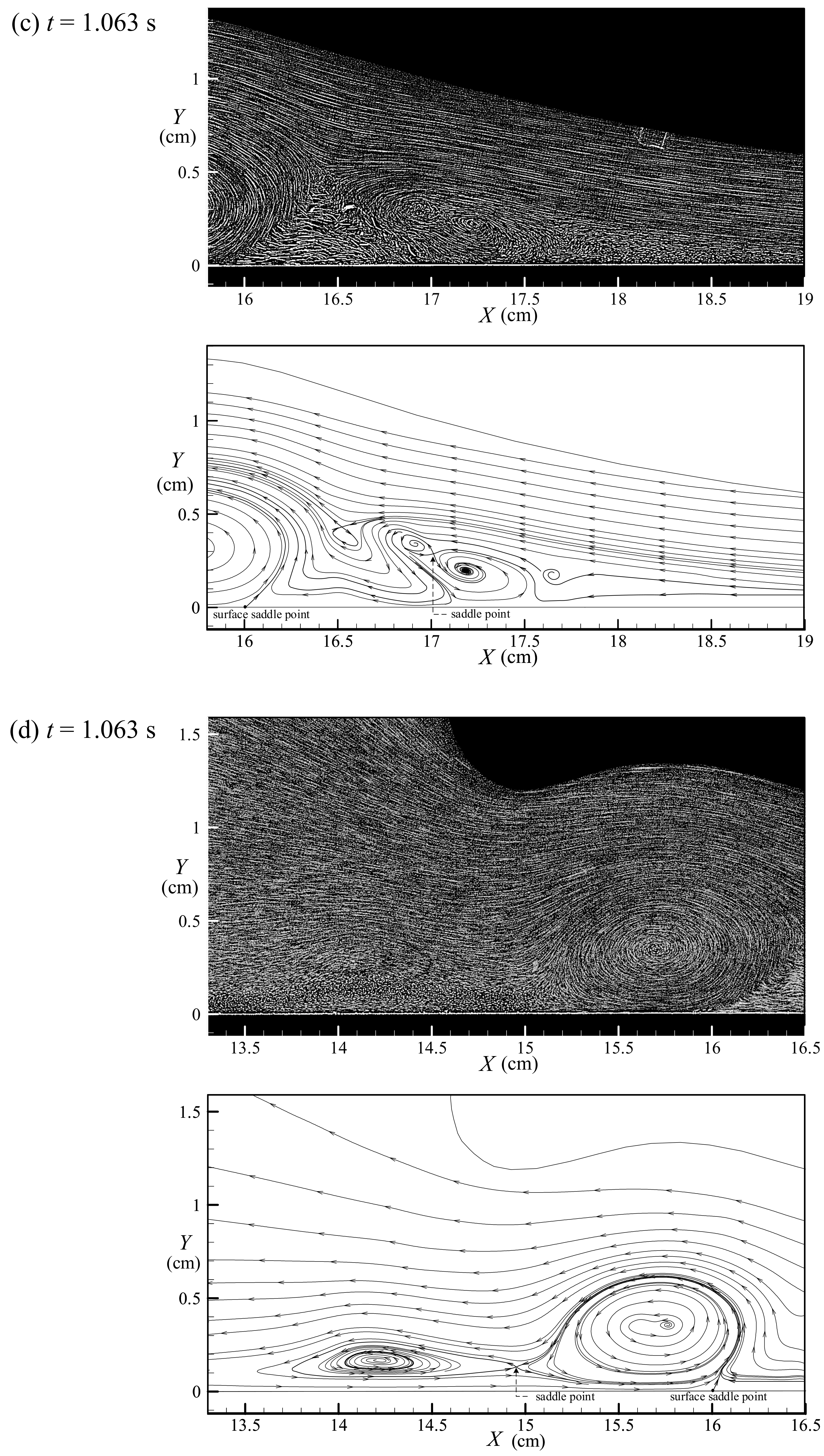
5.6. Second-Half Middle Stage II of Run-Down for 1.007 s < t ≤ 1.063 s

The free surface profile for t = 1.017 s, as shown in Figure 5b, soon after occurrence of hydraulic jump highlights the start of the curling jet with the tongue-shaped free surface moving “offshore.” Figure 15a presents the corresponding visualized image (on the top panel) and streamline pattern (on the bottom panel) for 15.80 cm ≤ X ≤ 19.00 cm, emphasizing the primary vortex. The primary vortex has a well-organized structure with the size height of Y_size = 0.40 cm and the core section at X_co = 17.20 cm. This core section is located on the onshore side of the critical section at X_cr = 16.12 cm (not shown), indicating occurrence of a supercritical flow at the core section. Two developing minor vortices rotating in the counterclockwise and clockwise directions are located on the offshore and onshore sides of the primary vortex for 15.8 cm ≤ X ≤ 16.4 cm and 17.6 cm ≤ X ≤ 18.1 cm, respectively. These two minor vortices are formed under separated shear layer with continuous energy supply from the accelerated, supercritical retreated flow. Two saddle points are seen evidently on both sides of the primary vortex, with one being located at about (X, Y) = (16.45, 0.1) cm and the other at (18.0, 0.17) cm. Moreover, a surface saddle point (Hunt et al. [43]) is identified at about (X, Y) = (17.5, 0) cm with one virtual streamline orienting upward from the bottom surface; and a stagnation point is observed at (X, Y) = (18.08, 0) cm with a streamline directing toward the beach surface. These observations exhibit, remarkably, a developing topological structure under the separated shear layer.

Figure 15b illustrates the visualized image (on the top panel) and streamline pattern (on the bottom panel) for 15.80 cm ≤ X ≤ 19.00 cm at t = 1.048 s, at which the projecting jet, consequent from the curling jet on the tip of free surface, is developing (also see Figure 5b). Due to persistent acceleration of the external stream in the supercritical retreated flow, the primary vortex subsequently evolves with further formation of the secondary and finer vortices beneath the separated shear layer for 16.8 cm ≤ X ≤ 17.8 cm. According to the principle of topological structure reported by Hunt et al. [43], a multi-vortex complex structure consisting of a series of vortices with critical point(s) (e.g., saddle, nodal, or stagnation point) in between keeps developing under the separated shear layer and moves offshore. For t = 1.048 s, the core section is located at X_co = 16.31 cm which is more onshore than that of the critical section (X_cr = 15.25 cm). Meanwhile, the size height is about Y_size = 0.57 cm, equal to half of the local water depth (i.e., h’/2 = 0.59 cm) approximately and greater than those for t = 0.983–1.017 s. Furthermore, Figure 15c shows the corresponding evolution of the secondary and finer vortices that move further offshore for 15.80 cm ≤ X ≤ 19.00 cm at t = 1.063 s. To provide more profound observation of the main structure in the primary vortex, a FOV ranging further offshore between X = 13.3 cm and X = 16.5 cm is used additionally. Figure 15d shows the primary vortex extending from X = 15.1 cm to X = 16.4 cm with the size height of Y_size = 0.64 cm and the core section at X_co = 15.7 cm for t = 1.063 s. The two images taken at the same t (Figure 15c,d) strongly demonstrate nearly identical flow structure existing in the overlapped region for 15.8 cm ≤ X ≤ 16.5 cm, and very high repeatability of the generated solitary wave over the sloping beach.

5.7. Late Stage of Run-Down for 1.063 s < t < 1.213 s

As depicted in Figure 5b for t = 1.048 and 1.077 s, the descent of projecting jet with some advancement in its tip as well as prominent drawn-back in the waist portion can be evidenced. Figure 16a,b shows the visualized image (on the top panel) and streamline pattern (on the bottom panel) of the flow field for t = 1.077 s. The result reveals that the primary vortex with a size height of Y_size = 0.70 cm moves toward offshore and interacts with a vortex located on its offshore side, undergoing a process of merging in 13.3 cm ≤ X ≤ 14.25 cm. The core of the primary vortex is located at X_co = 14.98 cm, which is more toward offshore, as compared with that for t = 1.048 s (i.e., at X_co = 16.31 cm). In addition, the external stream of the retreated flow appearing beneath the moving free surface and beyond the primary vortex is also observed. Figure 16c also presents four velocity profiles obtained at X = 16.25 cm, 15.59 cm, 14.98 cm (=X_co), and 14.36 cm. Due to the existence of the hump-shaped free surface profile over the external stream, the local water depths at these four sections vary very drastically. The mean velocity of the external stream, U_ex, can be obtained by partially depth-averaging over the velocity data beneath the free surface and just beyond the most outside streamline surrounding the primary vortex (see Figure 16b). Accordingly, the mean velocity of the external stream are in the order U_ex = −74.7, −101.6, −54.0, and −101.7 cm/s. Nevertheless, the fully depth-averaged velocities are correspondingly equal to U_d = −71.6, −49.1, −47.9, and −45.3 cm/s, demonstrating deceleration of the retreated flow in the offshore direction. In addition, the Froude numbers F_r, as shown in Figure 16a (marked over the four dashed lines), are larger than unity, revealing that the retreated flow is still supercritical up to t = 1.077 s.

Further, the convection velocity of the primary vortex core, U_cv, is defined as the mean velocity of the vortex core transported in the offshore direction within a specified time elapse. For t = 1.048 s, the convection velocity can be estimated from the visualized images for t = 1.040–1.057 s to be U_cv = −53.1 cm/s. It is also found that the magnitude of this convection velocity U_cv is, in fact, less than any one of the four mean velocities of the external stream, U_ex (also shown in the top of Figure 16a). Namely, the high-speed external stream, which has higher offshore speed, translates rapidly over the vortex with distinguishable curvature on the onshore side of the primary vortex, and “impinges upon” the primary vortex due to the relative obstruction of the primary vortex moving with lower convection velocity. The high-speed external stream also acts like a free-jump flow surrounding and over the primary vortex then behaves like a free-flop flow sliding down the primary vortex.

As observed from continuous images, the projecting jet before impinging and right touching the free surface of the supercritical retreated flow can be evidenced in Figure 17a,b for 13.3 cm ≤ X ≤ 16.5 cm at t = 1.091 and 1.094 s, respectively. Soon afterward, the vortex with air core being enclosed, rotating clockwise, is generated at t = 1.098 s (see Figure 17c). This fact highlights the formation of two-phase flow field for t > 1.094 s during the late stage of run-down. Figure 17d presents the visualized image of the vortical flow within a further offshore region of 10.8 cm ≤ X ≤ 14.0 cm also at t = 1.098 s, indicating that the upper primary vortex interacts with the lower minor vortex. Merging of these two upper and lower vortices is undergoing. The core position of the primary vortex has moved from X_co = 16.31 cm at t = 1.048 s, via X_co = 14.98 cm at t = 1.077 s, then to X_co = 13.40 cm at t = 1.098 s. Soon after a short time interval, say at t = 1.134 s, the merged vortex has been carried more offshore and upward by the turbulent stream induced by the high-speed retreated flow. Very chaotic flow field in the neighborhood of the merged vortex is observed hereafter.

5.8. Second Run-Up for t ≥ 1.213 s

During a time elapse of 0.206 s after occurrence of hydraulic jump at t = 1.007 s, the corresponding free surface profile at t = 1.213 s is presented in Figure 5b. The tail-end of the free surface of the retreated flow has reached its offshore-most position at x = 18.0 cm during a complete evolution of run-down motion for t = 0.655–1.213 s, substantiating the end of the run-down and the start of the second run-up. It should be emphasized that the flow fields at this stage and beyond are very turbulent at least under the influence of the following serial events: (1) Flow impingement between the projecting jet and the supercritical retreated flow; (2) formation of the two-phase vortex (with air core being enclosed); (3) irregular deformation of air bubbles or air core, random rising of air bubbles due to the buoyancy effect; and (4) the turbulence induced by the air-bubble’s wake during the rising process (Lin et al. [44]).

6. Discussion on Characteristics of Primary Vortex Structure

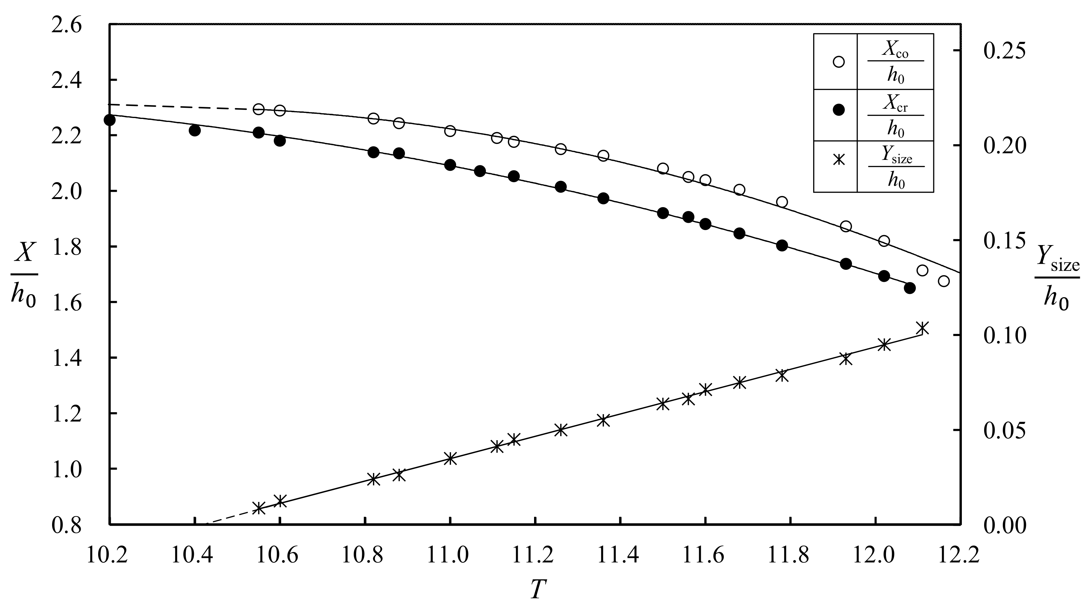
6.1. Variations of Critical and Core Sections as Well as Size Height for 10.20 ≤ T ≤ 12.11

Up to now, temporal variation of the critical section having F_r = 1.0 can be summarized for t = 0.921–1.094 s (i.e., T = 10.20–12.11) for Case 1. These data are all shown in the non-dimensional form of X_cr/h₀ versus T in Figure 18. Note that T = 10.20, the incipient flow separation occurs, and at T = 12.11, the projecting jet right impinges upon the free surface of the retreated flow. It strongly indicates that the critical section moves offshore as T increases for 10.20 ≤ T ≤ 12.11 as indicated in Figure 18 with a decrease in the value of X_cr/h₀. This is due to the vortex being enclosed with air core, thus leading to the two-phase flow field with a larger water depth. Later, with T ≥ 12.11, the critical section no longer exists. Figure 18 also illustrates the temporal variation of the non-dimensional size height Y_size/h₀, clearly indicating that the size height of the primary vortex increases linearly by increasing T for 10.55 ≤ T ≤ 12.11.

Summary of the temporal variation in the non-dimensional shoreward distance of the core section X_co/h₀ is also illustrated in Figure 18. It is shown that the primary vortex core moves offshore as T increases for 10.55 ≤ T ≤ 12.11, and that the core section appears on the onshore (i.e., shallower) side of the critical section at the identical T. Remember that, soon after the incipient flow separation at T = 10.20 (t = 0.921 s, see Figure 11b–d), a very thin flow reversal zone underlying the shear layer develops for 10.20 < T < 10.55. During this interval, the core of the elongated recirculation zone is hardly recognized. However, for T ≥ 10.55, the primary vortex evolved from the elongated recirculation zone can be identified, see Figure 12a–d for T = 10.60–10.88 (t = 0.957–0.983 s).

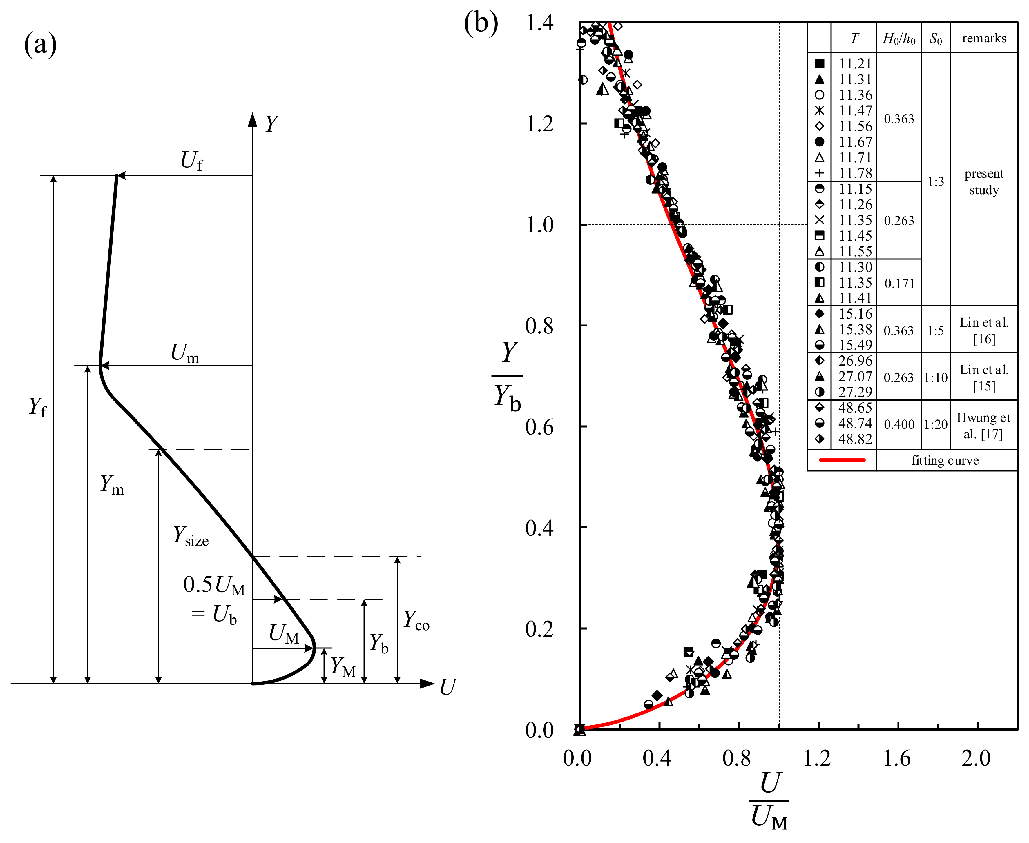
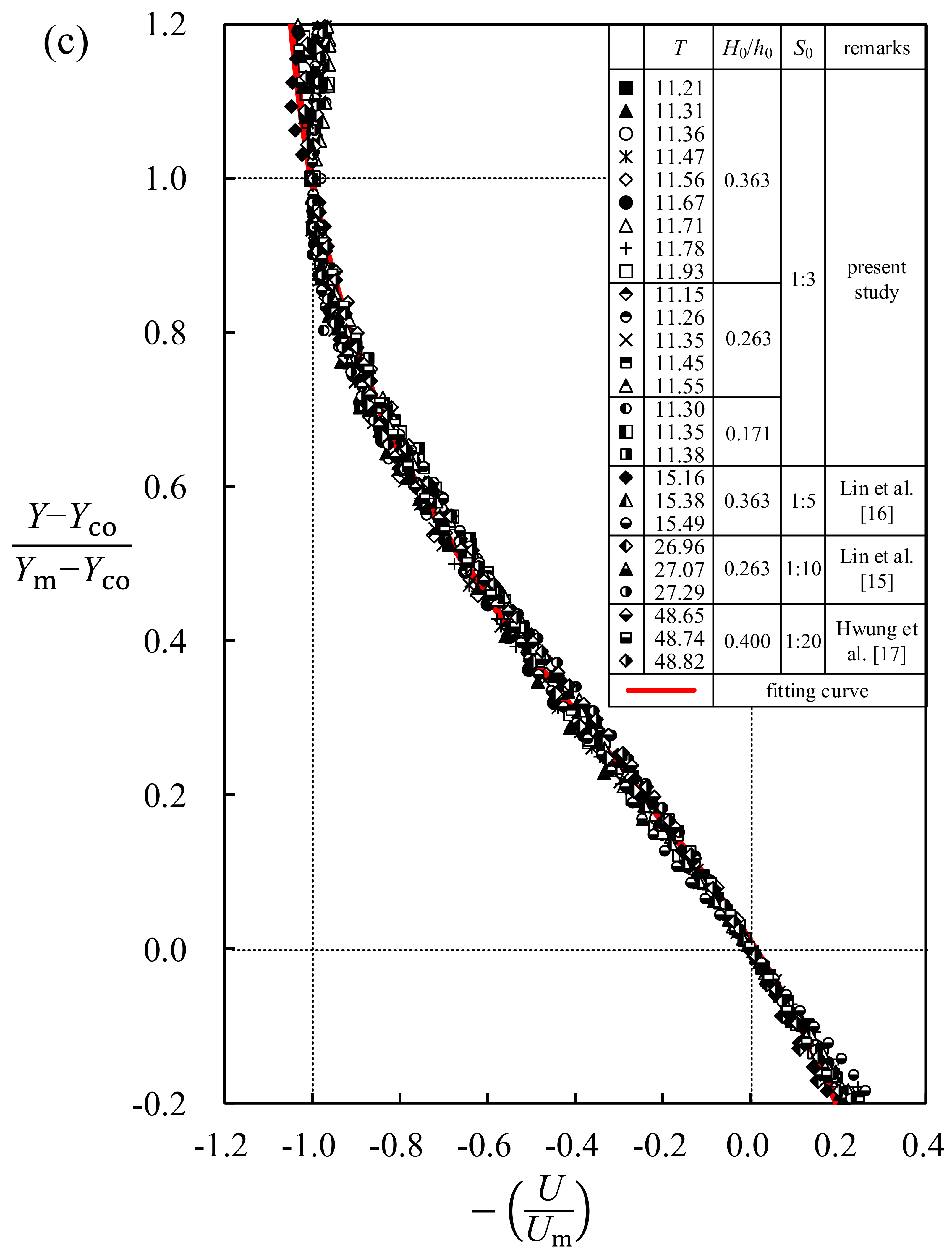
6.2. Similarity Profiles for Velocity Distributions at Core Sections for 11.00 < T < 12.11

As seen in Figure 14b for t = 1.007 s (T = 11.15) and the sub-figure ② of Figure 16c for t = 1.077 s (T = 11.93), a schematic diagram of the velocity profiles U(Y) passing through the primary vortex core at different t is shown in Figure 19a. Herein, Y_M denotes the height at which the maximum onshore velocity U_M (> 0) occurs and Y_co represents the core height of the primary vortex where U is equal to zero, i.e., U = U_co = 0. Further, Y_m represents the height where the negative maximum velocity U_m (< 0) occurs, and U_f (< 0) stands for the velocity nearly at the free-surface height, Y_f. Note that the velocity profile, U(Y), shows the uniform feature if U_m is equal to U_f for Y_m ≤ Y ≤ Y_f. However, if U_m occurs at the free-surface height Y_f, i.e., U_m = U_f, the velocity profile then exhibits the velocity gradient or non-uniform distribution for Y_co ≤ Y ≤ Y_f. It should be emphasized that, for 0 < Y ≤ Y_co, the velocity distribution is significantly influenced by the existence of the sloping beach and somehow exhibits a wall jet feature. On the other hand, the velocity profile U(Y) between Y = Y_co and Y = Y_m (or Y = Y_f if U_m = U_f) has the characteristics of shear layer between Y_co and Y_m or Y_f. Based on the interpretation mentioned above, two non-dimensional profiles for the velocity distributions U(Y) are proposed: One for the wall jet flow and the other for the shear layer flow.

For the first one that occurs close to the sloping beach, the maximum onshore velocity U_M and the height Y = Y_b where U = U_M/2 = 0 cm/s take places at the “half thickness” are taken as the characteristic velocity and length scales, respectively (Rajaratnam [45]). The data from not only Case 1 (with H₀/h₀ = 0.363), but also Cases 2 and 3 (with H₀/h₀ = 0.263 and 0.171, examples see Figure A1 in Appendix A) are all considered. Then, a non-dimensional profile for the velocity distributions that are close to the sloping beach, U(Y) (passing through the primary vortex core at different T), can be obtained by scaling with respect to these two characteristic scales. Figure 19b presents the non-dimensional plot for the present three cases, strongly highlighting a unique trend with a promising similarity, independent of the incident wave-height to water-depth ratio. However, to achieve a systematic summary for the effect of the beach slope, the data from Hwung et al. [17] for S₀ = 1:20 and Lin et al. [15,16] for S₀ = 1:10 and 1:5 (in which the global velocity fields were all demonstrated, but the details associated with vortex structures were not shown) are especially included in Figure 19b, via the similar rescaling process. It is surprisingly found that the trend of the data points from these three studies are almost identical to that of the present three cases, evidently indicating no effect of beach slope and wave-height to water-depth ratio on this similarity profile. Regression analysis for all of the data points illustrates that the universal similarity profile for the non-dimensional velocities, U(Y)/U_M, can be uniquely expressed as

U(Y)/U_M = 3.30(Y/Y_b − 0.02)^0.65 × {1.0 − erf(1.02(Y/Y_b − 0.02))} − 0.03 for 0 < Y/Y_b ≤ 1.4,

(4)

in which erf( ) is the error function. The regressed curve fits fairly well the data trend having a R² value of 0.982. This emphasizes that both the wave-height to water-depth ratio and the beach slope have no effect on the wall jet similarity profile. The present form of Equation (4) for the similarity profile of the onshore velocity is very similar to Verhoff’s velocity distribution equation for the traditional plane wall jet (Rajaratnam [45]; and Verhoff [46]), demonstrating the stream within the region between the core height and the sloping beach being the wall jet flow.

Regarding the second profile for the shear layer flow extending approximately from Y = Y_co to Y = Y_m (see Figure 19a), the representative velocity and length scales, −U_m (> 0) and (Y_m − Y_co) are used to formulate an appropriate similarity profile. Note that (Y_m − Y_co) stands for the representative thickness of shear layer. Herein, the same data sets used in Figure 19b have also been incorporated in the analysis. Accordingly, the dimensionless re-scaled velocity profile, −U/U_m (<0), against the dimensionless re-scaled thickness, Y* = (Y − Y_co)/(Y_m − Y_co), is plotted in Figure 19c with the non-linearly regressed fitting (R² = 0.997) as:

−U/U_m = −0.760 × tanh(1.869Y* − 0.484) − 0.331        for 0 ≤ Y* ≤ 1.0,

(5)

The above result exhibits a universal similarity profile for the velocities in the full thickness of the shear layer flow, again demonstrating neither the wave-height to water-depth ratio nor the beach slope has effects on this similarity profile. It should be indicated that Equation (5) is not only similar to those of the velocity distributions of the free and cavity shear layer flows (Michalke [47]; and Kuo et al. [48]), but also to the counterparts of a separated shear layer downstream of a submerged vertical plate or rectangular cylinder over which a solitary wave travels (Lin et al. [49,50]).

7. Conclusions

The evolutions of velocity field and vortex structure of the retreated flows on the offshore side of the still-water shoreline during run-down phase of non-breaking solitary waves, propagating over a 1:3 sloping beach, have been elucidated for Case 1 using two flow visualization techniques and HSPIV measurement system. The findings emphasize occurrences of the incipient flow separation and hydraulic jump, temporal variation in the shoreward position of critical section (with F_r = 1.0), and development of the primary vortex structure in terms of variations in size height, core section, and topological structure. Some important findings are drawn as follows:

• The run-down process of the solitary wave for 7.25 ≤ T < 13.43 can be divided into the early, middle, and late stages. In the early and first-half middle stage for about 7.25 ≤ T < 10.20, formation of the very streamlined free surface characterizes the flow event, highlighting the flow being decelerated in the offshore direction and subjected to adverse pressure gradient. The section of occurrence of the critical Froude number moves offshore as T increases for T > 9.00.
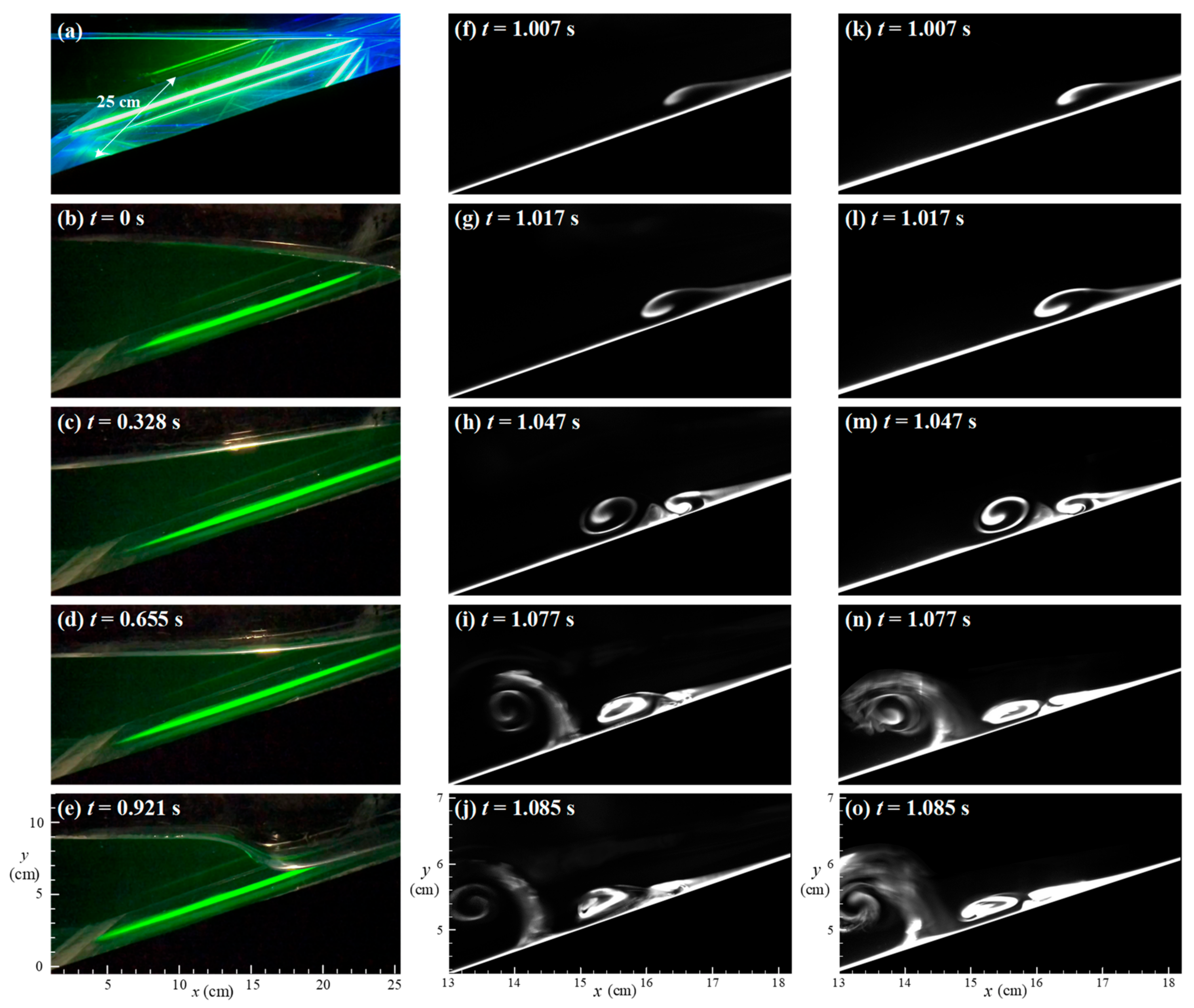
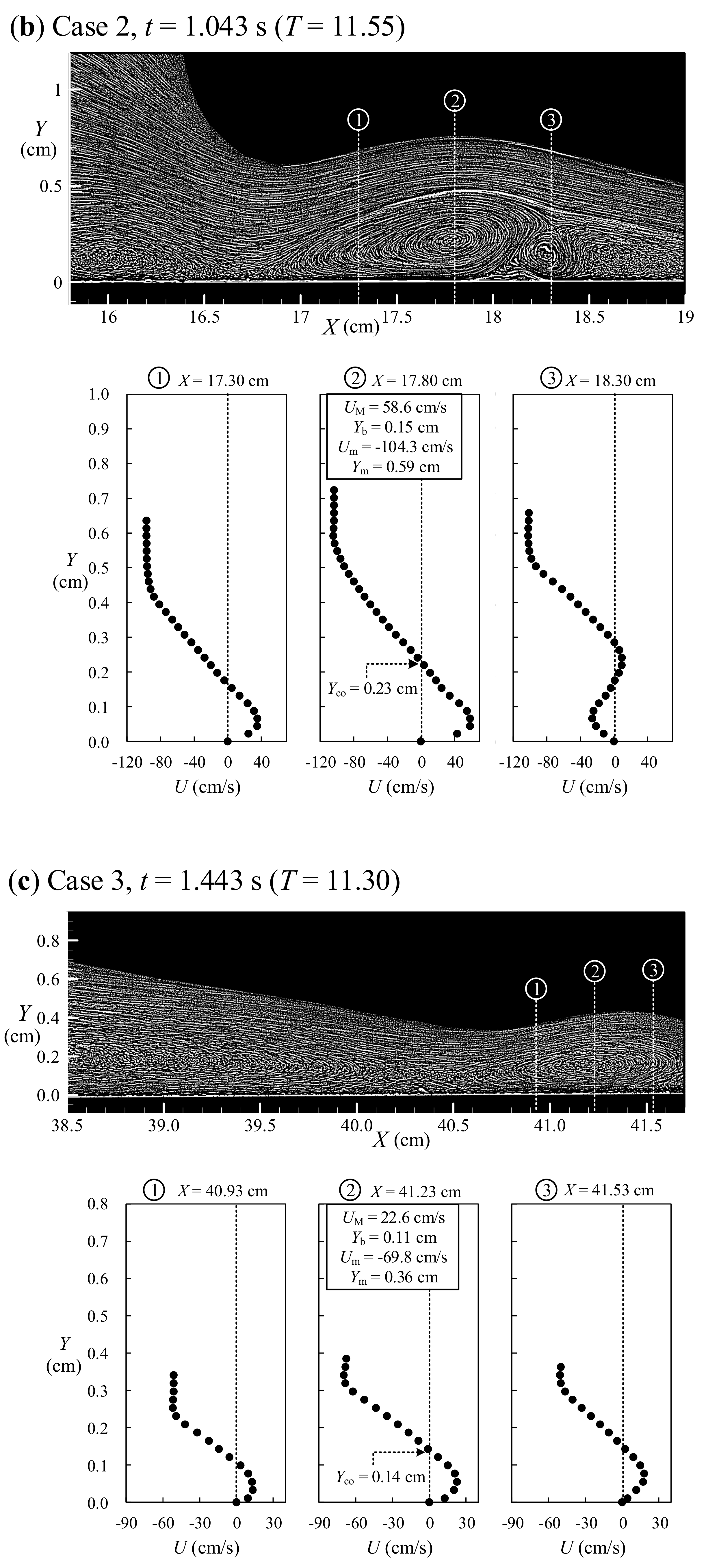
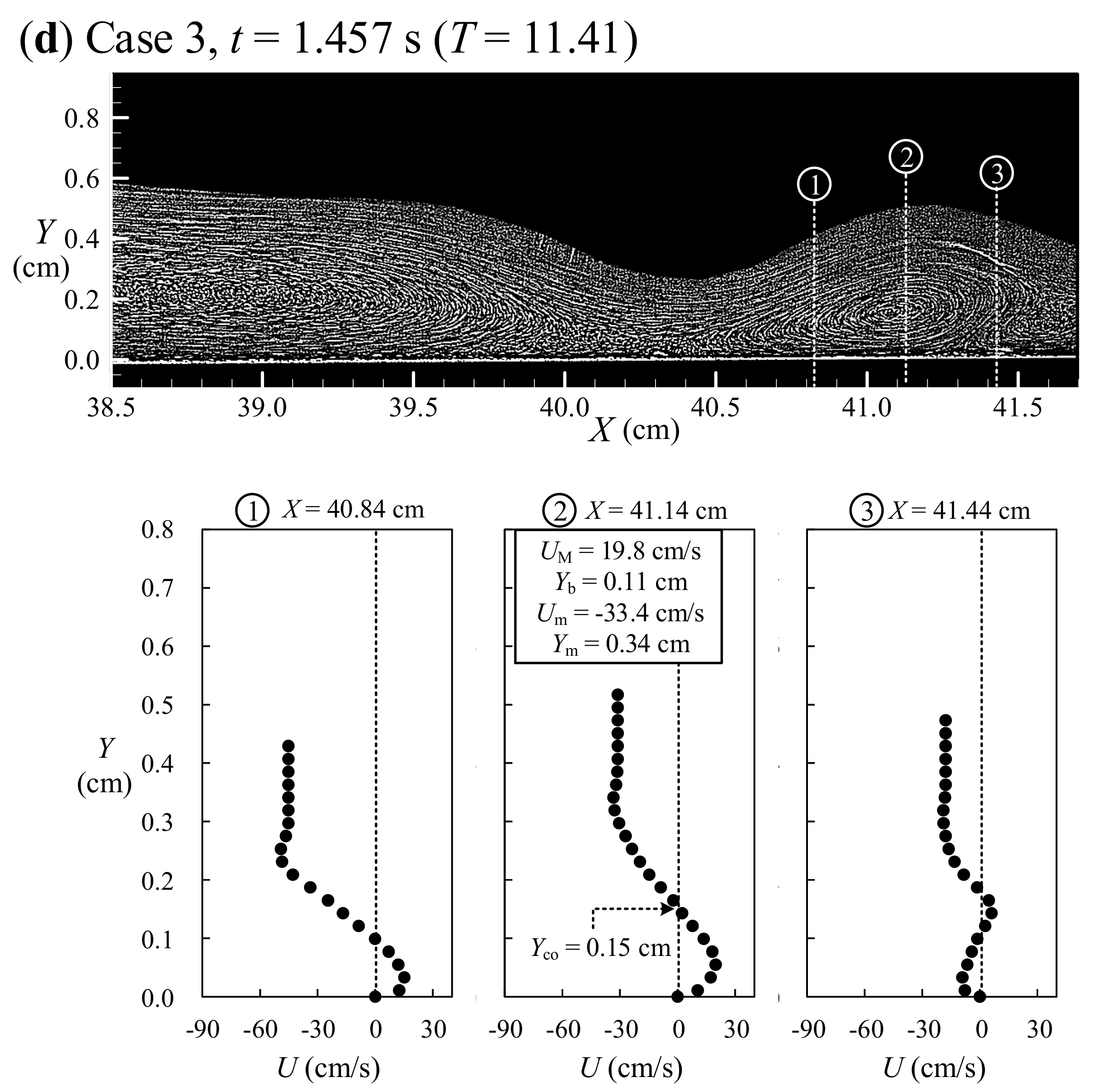
• In the second-half middle stage of the run-down process for 10.20 ≤ T < 11.60, the incipient flow separation, evolution of the primary vortex structure, hydraulic jump with sudden rising of the free surface in the retreated flow, and formation of curling jet on the upper portion of free surface take place sequentially.
• As regards the late stage of run-down process with 11.60 ≤ T < 13.43, transformation of the curled free surface into the impinging jet impacting on the free surface of the retreated flow at T = 12.11, and the two-phase flow with air core and/or subsequent air bubbles being entrained into vortex occur. Right at T = 13.43, the free surface of the retreated flow reaching its offshore-most position identifies the end of the run-down process.
• The non-dimensional shoreward distance of the critical/core section moves offshore as T increases for 10.2/10.55 ≤ T ≤ 12.11, with the latter taking place on the onshore side of the former for the identical T. The magnitudes of the non-dimensional size height of the primary vortex increases linearly with increasing T for 10.55 ≤ T ≤ 12.16. As a result of entrainment of air core within vortex, the two-phase flow field develops with a larger water depth for T ≥ 12.11, and consequently the critical section no longer exists.
• A unique similarity profile for the onshore velocity U(Y) measured through the primary vortex core and obtained very close to beach surface for 0 ≤ Y ≤ Y_co has been achieved by selecting the positive maximum velocity U_M and the specified half thickness Y_b as the characteristic velocity and length scales, respectively. This profile, with Equation (4), is very similar to Verhoff’s velocity distribution equation for the traditional plane wall jet, demonstrating existence of the wall jet flow right beyond the beach surface.
• Further, a similarity profile for the offshore velocity U(Y) in the shear layer, obtained between the core height of the primary vortex Y_co and the specified height Y_m, has been realized by selecting the negative maximum velocity U_m and the representative thickness of the shear layer (Y_m − Y_co) as the characteristic velocity and length scales, respectively. This profile, with Equation (5), identifies the feature of the shear layer flow, similar to those of traditional velocity distributions in the free and cavity shear layer flows.
• The two similarity profiles obtained for wall jet flow very close to the beach surface (0 ≤ Y ≤ Y_co) and for shear layer flow between the core height of the primary vortex Y_co and the specified height Y_m are obtained considering all of the three cases of the present study (H₀/h₀ = 0.171, 0.263, and 0.363) as well as data of Lin et al. [15,16] for S₀ = 1:10 and 1:5 and Hwung et al. [17] for S₀ = 1:20. This is evidence that neither the wave-height to water-depth ratio H₀/h₀ nor the beach slope S₀ has effects on both the wall jet and shear layer similarity profiles, strongly highlighting their universal feature.

It is expected that all of the results presented above can be regarded as a data bank and used to improve/verify the state-of-the-art or future numerical models step-by-step temporally.

References

1. British Association for the Advancement of Science. Committee on Waves. In Report of the Committee on Waves: Appointed by the British Association at Bristol in 1836 [and Consisting of Sir John Robison and John Scott Russell]; R. and J.E. Taylor: London, UK, 1838; pp. 417–496. [Google Scholar]
2. United States. Beach Erosion Board. Laboratory Investigation of the Vertical Rise of Solitary Waves on Impermeable Slopes; U.S. Beach Erosion Board: Washington, DC, USA, 1953.
3. Synolakis, C.E. The runup of solitary waves. J. Fluid Mech. 1987, 185, 523–545. [Google Scholar] [CrossRef]
4. Zelt, J.A. The run-up of nonbreaking and breaking solitary waves. Coast. Eng. 1991, 15, 205–246. [Google Scholar] [CrossRef]
5. Grilli, S.T.; Subramanya, R.; Svendsen, I.A.; Veeramony, J. Shoaling of solitary waves on plane beaches. J. Waterw. Port Coast. Ocean Eng. 1994, 120, 609–628. [Google Scholar] [CrossRef]
6. Grilli, S.T.; Svendsen, I.A.; Subramanya, R. Breaking criterion and characteristics for solitary waves on slopes. J. Waterw. Port Coast. Ocean Eng. 1997, 123, 102–112. [Google Scholar] [CrossRef]
7. Lin, P.; Chang, K.A.; Liu, P.L.F. Runup and rundown of solitary waves on sloping beaches. J. Waterw. Port Coast. Ocean Eng. 1999, 125, 247–255. [Google Scholar] [CrossRef]
8. Li, Y.; Raichlen, F. Energy balance model for breaking solitary wave runup. J. Waterw. Port Coast. Ocean Eng. 2003, 129, 47–59. [Google Scholar] [CrossRef]
9. Jensen, A.; Pedersen, G.K.; Wood, D.J. An experimental study of wave run-up at a steep beach. J. Fluid Mech. 2003, 486, 161–188. [Google Scholar] [CrossRef]
10. Hsiao, S.C.; Hsu, T.W.; Lin, T.C.; Chang, Y.H. On the evolution and run-up of breaking solitary waves on a mild sloping beach. Coast. Eng. 2008, 55, 975–988. [Google Scholar] [CrossRef]
11. Sumer, B.M.; Sen, M.B.; Karagali, I.; Ceren, B.; Fredsøe, J.; Sottile, M.; Zilioli, L.; Fuhrman, D.R. Flow and sediment transport induced by a plunging solitary wave. J. Geophys. Res. 2011, 116. [Google Scholar] [CrossRef] [Green Version]
12. Lo, H.Y.; Park, Y.S.; Liu, P.L.F. On the run-up and back-wash processes of single and double solitary waves—An experimental study. Coast. Eng. 2013, 80, 1–14. [Google Scholar] [CrossRef]
13. Pedersen, G.; Lindstrom, E.; Bertelsen, A.F.; Jensen, A.; Laskovski, D. Runup and boundary layers on sloping beaches. Phys. Fluids 2013, 25, 012102. [Google Scholar] [CrossRef]
14. Lin, C.; Yeh, P.H.; Hseih, S.C.; Shih, Y.N.; Lo, L.F.; Tsai, C.P. Pre-breaking internal velocity field induced by a solitary wave propagating over a 1:10 slope. Ocean Eng. 2014, 80, 1–12. [Google Scholar] [CrossRef]
15. Lin, C.; Yeh, P.H.; Kao, M.J.; Yu, M.H.; Hseih, S.C.; Chang, S.C.; Wu, T.R.; Tsai, C.P. Velocity fields in near-bottom and boundary layer flows in pre-breaking zone of solitary wave propagating over a 1:10 slope. J. Waterw. Port Coast. Ocean Eng. 2015, 141, 04014038. [Google Scholar] [CrossRef]
16. Lin, C.; Kao, M.J.; Tzeng, G.W.; Wong, W.Y.; Yang, J.; Raikar, R.V.; Wu, T.R.; Liu, P.L.F. Study on flow fields of boundary-layer separation and hydraulic jump during rundown motion of shoaling solitary wave. J. Earthq. Tsunami 2015, 9, 154002. [Google Scholar] [CrossRef]
17. Hwung, H.H.; Wu, Y.T.; Lin, C. Tsunami propagation and related new approach of mitigation. In Proceedings of the 8th Taiwan-Japan Joint Seminar on Natural Hazard Mitigation, Kyoto, Japan, 7 December 2015. [Google Scholar]
18. Skene, D.M.; Bennetts, L.G.; Wright, M.; Meylan, M.H.; Maki, K.J. Water wave overwash of a step. J. Fluid Mech. 2018, 839, 293–312. [Google Scholar] [CrossRef]
19. Higuera, P.; Liu, P.L.F.; Lin, C.; Wong, W.Y.; Kao, M.J. Laboratory-scale swash flows generated by a non-breaking solitary wave on a steep slope. J. Fluid Mech. 2018, 847, 186–227. [Google Scholar] [CrossRef]
20. Lin, C.; Hwung, H.H. Observation and measurement of the bottom boundary layer flow in the prebreaking zone of shoaling waves. Ocean Eng. 2002, 29, 1479–1502. [Google Scholar] [CrossRef]
21. Goring, D.G. Tsunami: The Propagation of Long Waves onto a Shelf; Technical Report No. KH-R-38; W. M. Keck Laboratory of Hydraulics and Water Resources, California Institute of Technology: Pasadena, CA, USA, 1978. [Google Scholar]
22. Adrian, R.J.; Westerweel, J. Particle Image Velocimetry; Cambridge University Press: New York, NY, USA, 2011. [Google Scholar]
23. Cowen, E.A.; Monismith, S.G. A hybrid digital particle tracking velocimetry technique. Exp. Fluids 1997, 22, 199–211. [Google Scholar] [CrossRef]
24. Mori, N.; Chang, K.A. Introduction to MPIV-PIV Toolbox in Matlab. User Reference Manual. 2009, pp. 1–15. Available online: http://www.oceanwave.jp/softwares/mpiv/index.php?Download (accessed on 1 November 2018).
25. Adrian, R.J. Particle imaging techniques for experimental fluid mechanics. Annu. Rev. Fluid Mech. 1991, 23, 261–304. [Google Scholar] [CrossRef]
26. Dean, R.G.; Dalrymple, R.A. Water Wave Mechanics for Engineers and Scientists; World Scientific Publishing Co. Pte. Ltd.: Hackensack, NJ, USA, 1995. [Google Scholar]
27. Lin, C.; Yu, S.M.; Wong, W.Y.; Tzeng, G.W.; Kao, M.J.; Yeh, P.H.; Raikar, R.V.; Yang, J.; Tsai, C.P. Velocity characteristics in boundary layer flow caused by solitary wave traveling over horizontal bottom. Exp. Therm. Fluid Sci. 2016, 76, 238–252. [Google Scholar] [CrossRef]
28. Keulegan, G.H. Gradual damping of solitary waves. J. Res. Nat. Bur. Stand. 1948, 40, 487–498. [Google Scholar] [CrossRef]
29. Mei, C.C. The Applied Dynamics of Ocean Surface Waves; World Scientific Publishing Co. Pte. Ltd.: Singapore, 1989. [Google Scholar]
30. Lin, C.; Kao, M.J.; Wong, W.Y.; Shao, Y.P.; Fu, C.F.; Yuan, J.M.; Raikar, R.V. Effect of leading waves on velocity distribution of undular bore traveling over sloping bottom. Eur. J. Mech. Ser. B Fluids 2018. [Google Scholar] [CrossRef]
31. Chang, K.A.; Liu, P.L.F. Pseudo turbulence in PIV breaking wave measurements. Exp. Fluids 2000, 29, 331–338. [Google Scholar] [CrossRef]
32. Ho, T.C. Characteristics of Vortical Flow Fields Induced by Solitary Waves Propagating over Submerged Structures with Different Aspect Ratios. Ph.D. Thesis, Department of Civil Engineering, National Chung Hsing University, Taichung City, Taiwan, 2009. [Google Scholar]
33. Sumer, B.M.; Jensen, P.M.; Sørensen, L.B.; Fredsøe, J.; Liu, P.L.F.; Carstensen, S. Coherent structures in wave boundary layers. Part 2. Solitary motion. J. Fluid Mech. 2010, 646, 207–231. [Google Scholar] [CrossRef]
34. Persson, B.N.J.; Albohr, O.; Tartaglino, U.; Volokitin, A.I.; Tossatti, E. On the nature of surface roughness with application to contact mechanics, sealing, rubber friction and adhesion. J. Phys. Condens. Matter 2005, 17, 82. [Google Scholar] [CrossRef] [PubMed]
35. Engineering Tool Box. Available online: http://www.engineeringtoolbox.com/surface-roughness-ventilation-ducts-d_209.html (accessed on 1 November 2018).
36. Tennekes, H.; Lumley, J.L. A First Course in Turbulence; the MIT Press: Cambridge, MA, USA, 1972. [Google Scholar]
37. Daily, J.W.; Harleman, D.R.F. Fluid Dynamics; Addison-Wesley Publishing Company, Inc.: Boston, MA, USA, 1966. [Google Scholar]
38. Henderson, F.M. Open Channel Flow; Macmillan Publishing Company Inc.: New York, NY, USA, 1966; pp. 218–219. [Google Scholar]
39. Chow, V.T. Open-Channel Hydraulics; McGraw-Hill Book Company: Singapore, 1973; pp. 425–428. [Google Scholar]
40. Subramanya, K. Flow in Open Channels; McGraw-Hill Book Company: New York, NY, USA, 1986; pp. 204–206. [Google Scholar]
41. Schlichting, H. Boundary Layer Theory; McGraw-Hill Book Company: New York, NY, USA, 1979. [Google Scholar]
42. Lin, C.; Chiu, P.H.; Hsieh, S.J. Characteristics of horseshoe vortex system near a vertical plate-base plate juncture. Exp. Therm. Fluid Sci. 2002, 27, 25–46. [Google Scholar] [CrossRef]
43. Hunt, J.C.R.; Abell, C.J.; Peterka, J.A.; Woo, H.J. Kinematical studies of the flows around free or surface-mounted obstacles—Applying topology to flow visualization. J. Fluid Mech. 1978, 86, 179–200. [Google Scholar] [CrossRef]
44. Lin, C.; Hsieh, S.C.; Lin, I.J.; Chang, K.A.; Raikar, V.R. Flow property and self-similarity in steady hydraulic jump. Exp. Fluids 2012, 53, 1591–1616. [Google Scholar] [CrossRef]
45. Rajaratnam, N. Turbulent Jet; Elsevier Scientific Publishing Company: Amsterdam, The Netherlands, 1976. [Google Scholar]
46. Verhoff, A. The Two-Dimensional Turbulent Wall Jet without an External Free Stream; Report No. 626; Princeton University: Princeton, NJ, USA, 1963. [Google Scholar]
47. Michalke, A. The instability of free shear layers. Prog. Aerosp. Sci. 1972, 12, 213–239. [Google Scholar] [CrossRef]
48. Kuo, C.H.; Huang, S.H.; Chang, C.W. Self-sustained oscillation induced by horizontal cover plate above cavity. J. Fluids Struct. 2000, 14, 25–48. [Google Scholar] [CrossRef]
49. Lin, C.; Ho, T.C.; Chang, S.C.; Hsieh, S.C.; Chang, K.A. Vortex shedding induced by a solitary wave propagating over a submerged vertical plate. Int. J. Heat Fluid Flow 2005, 26, 894–904. [Google Scholar] [CrossRef]
50. Lin, C.; Chang, S.C.; Chang, K.A. Laboratory observation of a solitary wave propagating over a submerged rectangular dike. J. Eng. Mech. 2006, 132, 545–554. [Google Scholar] [CrossRef]
Figure 1. (a) Schematic diagrams indicating sloping beach model and two coordinate systems, together with deployment of two wave gauges and six fields of view, FOV1–FOV6, for HSPIV measurements; and (b) photo showing wave flume, high-speed digital camera, and part of sloping beach.
Water 10 01713 g001
Figure 2. Comparison of temporal variation of free surface elevation measured at x = −150.0 cm over constant water depth with that predicted by the theory (Case 1).
Water 10 01713 g002
Figure 3. (a,b) Spatial variations of external and near-bottom velocity fields measured over horizontal bottom at t’ = −0.135 and 0 s (i.e., T’ = −1.50 and 0), respectively; and (c,d) comparison of horizontal velocity profiles in boundary layer measured by HSPIV with those obtained by fiber-optic laser Doppler velocimetry (Ho [32]) for different non-dimensional times (Case 3). Note that wave height and still water depth for this study are H0 = 2.74 cm and h0 = 16.0 cm, and counterparts for Ho [32] are H0 = 1.20 cm and h0 = 7.0 cm, both having identical value of H0/h0 = 0.171.
Water 10 01713 g003
Figure 4. Repeatability tests of instantaneous free surface profile and velocity field of solitary wave over sloping beach at t = 1.048 s (T = 11.60): (ac) instantaneous images taken for three distinct runs; (d) comparison of ten instantaneous free surface profiles with ensemble-averaged one; (eg) instantaneous velocity field corresponding to (ac), respectively; and (h) ensemble-averaged velocity field acquired from ten repeated runs (Case 1). Note that the flow structures shown are not generated by breaking wave, but by hydraulic jump with a “backward” motion (also see Figure 5b).
Water 10 01713 g004
Figure 5. Temporal and spatial variations of free surface profile: (a) global view for 0 s ≤ t ≤ 1.351 s (0 ≤ T ≤ 14.96); and (b) magnified view for run-down process during time interval 1.007 s ≤ t ≤ 1.141 s (11.15 ≤ T ≤ 12.64) (Case 1).
Water 10 01713 g005
Figure 6. Chronological sketches for (a) complete evolution of run-up and run-down process; and (b) detailed classification for different stages of run-down process (Case 1).
Water 10 01713 g006
Figure 7. Flow visualized images: (a) Close-up of green dye strip (with nearly constant width) over beach surface, while water volume inside wave flume being kept quiescent; (be) dye strip transported onshore without changing its width in spanwise direction at five different times; (fj) flow structures on central vertical plane 12.5 cm away from front sidewall at five distinct times; (ko) the counterparts each with same time as that shown in (fj), respectively, and on vertical plane 8.0 cm away from front sidewall.
Water 10 01713 g007
Figure 8. (a) Spatial variation of velocity field at t = 0.655 s; (b) velocity profiles, u(y*), obtained at four different shoreward distances, x, as marked in (a) each with vertical line marked by circled number (Case 1). Note that the shifted height is denoted by y* = yx/3.
Water 10 01713 g008
Figure 9. Variation of horizontal uniform velocity with shoreward distance, together with a change of free surface profile for t = 0.655–0.983 s (Case 1).
Water 10 01713 g009
Figure 10. Velocity profiles, U(Y), measured at five different positions for t = 0.813 s (Case 1).
Water 10 01713 g010
Figure 11. (a) Spatial variation of velocity field at t = 0.921 s; (b) near-bottom velocity field obtained at t = 0.921 s; (c) three velocity profiles selected from (a), depicting incipiency of flow separation in boundary layer at X = 18.81 cm, as shown in sub-figure 2’; and (d) detailed comparison of three velocity profiles very close to the beach surface (Case 1).
Water 10 01713 g011
Figure 12. (a) Near-bottom velocity field at t = 0.957 s; (b) close-up of near-bottom velocity field for (a); (c) near-bottom velocity field at t = 0.983 s; and (d) close-up of near-bottom velocity field for (c) (Case 1).
Water 10 01713 g012
Figure 13. (a) Velocity field corresponding to occurrence of hydraulic jump; and (b) five velocity profiles U(Y) extracted from (a) and marked with values of Froude number for t = 1.007 s (Case 1).
Water 10 01713 g013
Figure 14. (a) Visualized image of retreated flow moving offshore; and (b) streamline pattern for t = 1.007 s (Case 1).
Water 10 01713 g014
Figure 15. Visualized image (on top panel) and streamlined pattern (on bottom panel) obtained at (a) t = 1.017 s; (b) t = 1.048 s; (c,d) t = 1.063 s. Note that the range on abscissa in (d) is different from that shown in (ac) for Case 1.
Water 10 01713 g015aWater 10 01713 g015b
Figure 16. For t = 1.077 s, (a) visualized image with external stream moving offshore; (b) streamlined pattern; and (c) four velocity profiles U(Y) measured at four different positions, as marked by dashed lines on (a).
Water 10 01713 g016
Figure 17. Visualized images of interaction process between projecting jet and retreated flow at (a) t = 1.085 s before jet impinging; (b) t = 1.094 s for jet right impinging on retreated flow; (c) t = 1.098 s for jet bifurcating into two substreams; and (d) t = 1.098 s for merging of vortices (Case 1).
Water 10 01713 g017
Figure 18. Variations in non-dimensional shoreward distances for critical and core sections as well as in non-dimensional size height (Case 1).
Water 10 01713 g018
Figure 19. (a) Schematic plot of velocity profile U(Y) passing through primary vortex core; and (b) universal similarity profile of wall jet flow close to beach surface for YYM; (c) universal similarity profile of shear layer flow between Y = YM and Y = Ym. Note that data from the present three cases for S0 = 1:3, Lin et al. [15,16] for S0 = 1:5 and 1:10, and Hwung et al. [17] for S0 = 1:20 have been included to highlight no effect of H0/h0 and S0 on these two unique profiles.
Water 10 01713 g019aWater 10 01713 g019b