Research on the Data-Driven Quality Control Method of Hydrological Time Series Data


1
College of Computer and Information, Hohai University, Nanjing 211100, China
2
Huawei Technologies Co., Ltd., Nanjing 210012, China
*
Author to whom correspondence should be addressed.
Water 2018, 10(12), 1712; https://doi.org/10.3390/w10121712
Submission received: 17 October 2018
/
Revised: 13 November 2018
/
Accepted: 21 November 2018
/
Published: 23 November 2018
(This article belongs to the Special Issue Enhancing Hydrological Prediction through Modelling with Large Datasets)
Abstract
:Ensuring the quality of hydrological data has become a key issue in the field of hydrology. Based on the characteristics of hydrological data, this paper proposes a data-driven quality control method for hydrological data. For continuous hydrological time series data, two combined forecasting models and one statistical control model are constructed from horizontal, vertical, and statistical perspectives and the three models provide three confidence intervals. Set the suspicious level based on the number of confidence intervals for data violations, control the data, and provide suggested values for suspicious and missing data. For the discrete hydrological data with large time-space difference, the similar weight topological map between the neighboring stations is established centering on the hydrological station under the test and it is adjusted continuously with the seasonal changes. Lastly, a spatial interpolation model is established to detect the data. The experimental results show that the quality control method proposed in this paper can effectively detect and control the data, find suspicious and erroneous data, and provide suggested values.
1. Introduction
In recent years, with the in-depth development of information technology and the overall promotion of water conservancy, China’s water conservancy information construction has gradually deepened. Water conservancy informatization is to make full use of information technology to improve the application level and development and sharing of information resources through the collection, transmission, storage, processing, and use of water conservancy data [1].
With efficient computing facilities, hydrological data has grown exponentially and flooded into hydrological real-time databases. Mining more practical and valuable information from big data is getting more and more attention with the rapid growth of hydrological data. In the big data mining of massive hydrological data, the accuracy and credibility of experiments and applications can be guaranteed only when the data quality problems such as missing and abnormal data are in the controllable range. However, the monitoring level of hydrological stations in China is in the transition from manual recording and semi-automatic to fully automated monitoring. During this period, there will be uncertainties such as installation and the upgrade of the automatic station acquisition system, monitoring sensor interference with measurement accuracy, abnormal jump of instruments caused by extreme weather, and so on. These factors cause anomalies as well as lacks and errors in hydrological data of many monitoring stations. Such erroneous and abnormal data records sometimes mislead disaster management judgment and lead to property losses. Therefore, how to ensure the normalization and accuracy of incoming data is a key issue in the field of hydrology.
Many scholars have proposed some schemes for the control, management, and evaluation of data quality in recent years. Sciuto et al. [2] relied on the consistency of temperature data, set the sliding window of 11 to use the Fourier transform to smooth the average and mean square error of the data in the window, and establish the maximum and minimum temperature confidence intervals to find the abnormal values in the data. Steinacker et al. [3] expounded the error types and introduced some basic data quality control methods (such as extremum detection, consistency detection, Bayesian quality control, and complex artificial auxiliary control). On this basis, he proposed a method to find the weights between stations by establishing topological structure of the station space position for the direction of artificial auxiliary control. Sciuto and Abbot [4,5] used the rainfall data of the surrounding stations to establish the neural network prediction model and set the confidence interval of the data and regarded the rainfall data outside the confidence interval as the outlier. Fangjing Fu and Xi Luo [6] respectively investigated and detected the hydrological data stored in the warehouse from the aspects of rationality, completeness, and consistency of the data including detecting the extreme range of data records and the consistency between the internal factors. Yu Yufeng [7] used Benford’s rule to analyze the distribution law of data in the hydrological database and to test the rationality of the hydrological dataset as a whole. On the basis of research, the established hydrological data quality model proposed a hydrological data quality improvement scheme combining automatic cleaning and manual cleaning [8] and expounded the basic data quality processing methods from five aspects: missing data processing, logical error detection, repeated data processing, abnormal data detection, and inconsistent data processing, which provide some ideas for hydrological data quality control.
However, there are still many problems in the quality control of hydrological data. For example, the hydrological data quality control methods in China are more in the theoretical research and modeling stage, lack of complete data quality control algorithms, and models for real-time control of hydrological data. Many papers [3,4,5,6,7,8] mention that basic data quality control methods such as logic checking, extremum checking, internal consistency checking, time consistency checking, and spatial consistency checking can detect the data with quality problems but do not give a reliable value or an effective method to replace the problem data. For hydrological data that is short-term missing due to machine failure, linear quality control interpolation methods such as the average method, the weighting method, or the spatial interpolation method are generally used for filling. However, the filling values vary according to the density of the data collected and the credibility of the filling data lacks the measurement scale.
To solve these problems, this paper proposes a data-driven quality control method for hydrological data. According to the continuity of data in time, the hydrological data is divided into two types: continuous type and discrete type. The corresponding control models are established for different types of data to detect and control the real-time monitored data and to analyze and identify problem data such as abnormalities, errors, and redundancy from the point of view of data and expert knowledge to ensure the quality of hydrological data and to provide data support for hydrologists to conduct data mining analysis and decision-making. This article works as follows:
- For continuous data, two stable predictive control models, i.e. the horizontal optimized integrated predictive control model and the longitudinal predictive control model, are constructed from the horizontal and vertical perspectives. The model provides two predictive values and confidence intervals for suspicious data and it is up to the staff to decide whether to manually fill, recommend replacement, or retain the original value. The latest data is used as a sample set for periodic training and model adjustment, so that the model parameters can be dynamically updated with time. The predicted values of the two models are used to set the control interval at the center to detect and control the quality of continuous hydrological data. Establish the statistical data quality control interval from the perspective of statistics, combine horizontal and vertical predictive control models, and propose the continuous hydrological data control model. The hourly hydrological real-time data is detected from the perspective of time consistency and the number of monitoring data violating the control interval is taken as its suspicion.
- For discrete hydrological data with a large spatial difference and poor temporal continuity (such as rainfall), a discrete hydrological data control scheme is proposed. Centered on the measured stations, a topological map of similarity weights between neighboring stations is established and adjusted with seasonal variation. The spatial interpolation model of daily precipitation is constructed by using the monitoring data of stations with a large correlation around and the missing precipitation data in the short term are attempted to be filled.
- Set the online real-time adjustment strategy, according to the seasonal variation characteristics of hydrology, and dynamically adjust the parameters of the basic QC parameters, thresholds, and parameters of the predictive control model when establishing the control interval.
2. Basic Theories Used in Hydrological Data Quality Control Model
2.1. Hydrological Data Quality Control Model
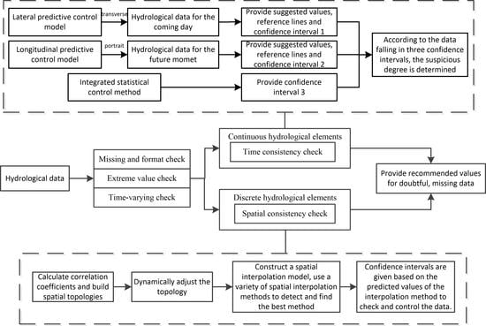
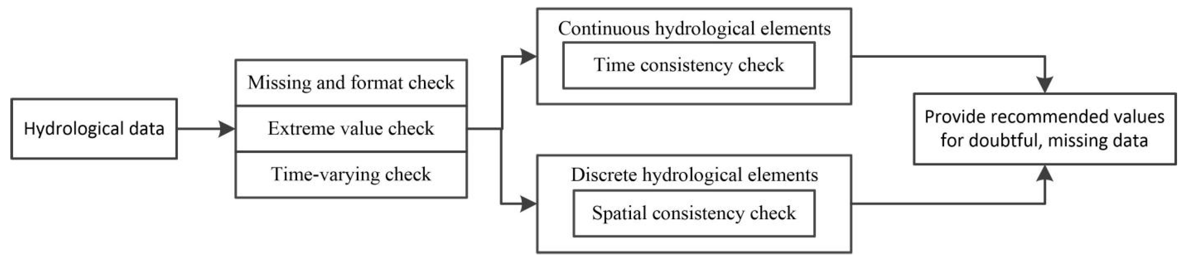
This paper reviews a set of quality control methods for hydrological data. On the basis of basic quality control (such as missing test and format check, extreme value check, and time-varying check), hydrological data are divided into two categories: continuous and discrete, which are checked and controlled separately. For continuous hydrological data, two combined predictive control models, one statistical control model, and the corresponding control interval are constructed to detect and control the hydrological factors such as the water level and discharge with good continuity from the horizontal, vertical, and statistical perspectives. For the suspicious data and the short-term missing data, the model provides the recommended value and confidence interval. For discrete hydrological data aiming at the disadvantage that rainfall data is difficult to control, this paper constructs the topological relation diagram of correlation coefficients centered on the measured stations and uses the spatial interpolation method based on the station data with large correlation coefficients to construct the spatial interpolation model and improve the prediction effect. The quality control framework proposed in this paper is shown in the Figure 1 below.
2.2. Related Theories
2.2.1. Definitions
Horizontal prediction: The process of predicting data at the same time of day m + 1 based on the data at the same time in the preceding m days.
Longitudinal prediction: The process of predicting data of (m + 1)th hour based on the data of the preceding m hours.
2.2.2. Prediction Methods
Recurrent Neural Network
The recurrent neural network (RNN) [9,10] is a popular learning method in the field of deep learning in recent years and is a kind of neural network for processing sequence data. Compared with the independent calculation results of common neural networks, the results of each hidden layer in RNN are correlated with the current input and the last hidden layer, that is, the input of hidden layer includes not only the output of the input layer but also the output of the previous hidden layer. However, RNN can only memorize part of the time series. Therefore, it is much shorter than long sequences. This results in the decrease of accuracy when the sequence is too long.
Support Vector Machines
Support Vector Machines (SVM) are developed for solving classification problems. It is a machine learning method based on the Vapnik-Chervonenkis Dimension theory and structural risk minimization [11]. Support Vector Regression (SVR) is a generalization of the SVM pattern recognition results in the regression domain. In the case of regression, an insensitive loss function Ɛ is introduced. If the error between the actual value and the predicted value is less than Ɛ, the loss is assumed to be zero. However, SVM merely transforms the difficulty of complexity in high-dimensional space to the difficulty of finding kernel functions. Even after determining the kernel function, quadratic programming is needed to solve the problem classification, which requires plenty of storage space.
Long-Short Term Memory
The Long-Short Term Memory model (LSTM) is a kind of Recurrent Neural Network (RNN) [10,12]. It proposes an improvement to the gradient disappearance problem in the RNN model and replaces the hidden layer nodes in the original RNN model with one memory unit. This memory unit consists of memory cells, forgetting gates, input gates, and output gates. The memory cells are responsible for storing historical information, recording, and updating historical information through a state parameter. The three gate structures determines the trade-off of information through the Sigmoid function, which acts on the memory cells.
2.2.3. Optimization Methods
Particle Swarm Optimization
Particle Swarm Optimization (PSO) [13,14,15,16] is a global optimization evolution algorithm proposed by Eberhart and Kennedy in 1995. The basic idea: Randomly initialize a group of particles, each of which flies at a certain speed in the search space, and evaluates the quality of the particles through a fitness function. The particle updates the speed by tracking the best solution found by the particle itself and the global best solution to fly to the position of the global best and find the optimal solution [17]. However, for functions with multiple local extremum points, it is easy to fall into the local extremum points and the correct results cannot be obtained.
Mind Evolutionary Algorithm
The Mind Evolutionary Algorithm (MEA) [18] is a global optimization algorithm that imitates human thinking. MEA inherits the idea of “group” and “evolution” of the Genetic Algorithm (GA) and innovates on this basis. It improves the search strategy in the process of population optimization and the evolutionary operator of evolutionary computation.
The core of MEA is convergence and alienation. Convergence refers to the process in which individuals compete to become winners in a subgroup and belong to local competition. Alienation is the process in which all subgroups compete with each other to become the winners in the whole space and constantly explore new points and replace the winners with temporary individuals with higher scores, which belong to global competition. For monotonic functions, MEA converges slowly around the optimal value. For multimodal functions, it converges to local optimum.
2.2.4. Statistical Methods
Adaptive Boosting
Adaptive Boosting (Adaboost) [19] is a representative algorithm in the Boosting family and it is one of the top 10 classical algorithms in the field of data mining. The algorithm idea is to train different weak classifiers for the same training set and then combine these weak classifiers to form a stronger final classifier. However, adaboost training is time consuming and requires re-selecting the best segmentation point for the current classifier each time.
Statistical Control
The horizontal statistical control refers to the process of establishing statistical confidence control for the data at the same time on the m + 1 day, according to the data of the same time in the previous m days by using the consistency of the time series.
The longitudinal statistical control refers to the process of establishing statistical confidence control for the data of m + 1 time, according to the real-time data of the previous m time of the history by using the consistency of the time series.
2.2.5. Spatial Interpolation Methods
The spatial interpolation methods mainly include inverse distance weighting, the trend surface method, the Kriging method, and other deformations. Each method has its scope of application and advantage. The trend surface method belongs to the global interpolation method while the other two methods belong to the local interpolation method [20,21].
Inverse Distance Weighting
Inverse Distance Weighting (IDW) was proposed by the National Meteorological Service of the United States in 1972. It uses the weighted average of observations from multiple stations to estimate the value of the estimated point. The magnitude of the weight depends on the square of the distance between the neighboring point and the estimated point [22]. It has low computational cost and universality and does not need to adjust the method, according to the characteristics of data. However, the size of IDW weight directly affects the size of standard deviation, determines the overall accuracy of interpolation, and has a significant impact on the interpolation results.
Trend Surface Method
The trend surface method uses the multiple regression method to analyze the spatial distribution characteristics of hydrological elements and constructs a curved surface to fit the trend and change of the elements [23]. That is to say, the hydrological factors are affected by two factors: the trend term and the random term in which the trend term reflects the overall change of the region and the random term reflects the local change characteristics of the region. However, interpolation is not good when sample points are sparse.
Kriging Method
The Kriging method is a spatial interpolation method commonly used on the basis of geostatistics. It is a method for finding the optimal, linear, and unbiased interpolation estimators of spatial distribution values [23]. Similar to the inverse distance weighting method, it is also a weighted average of local area estimates. However, the method is complicated, the calculation is large, and the operation speed is slow.
Some scholars introduced the nonlinear neural network and SVM technology into spatial precipitation interpolation and established a spatial interpolation model on this basis [20,21,22,23]. This paper will build a multi-variable SVM model and commonly used the spatial interpolation method for comparative analysis.
3. Continuous Hydrological Data Control Model
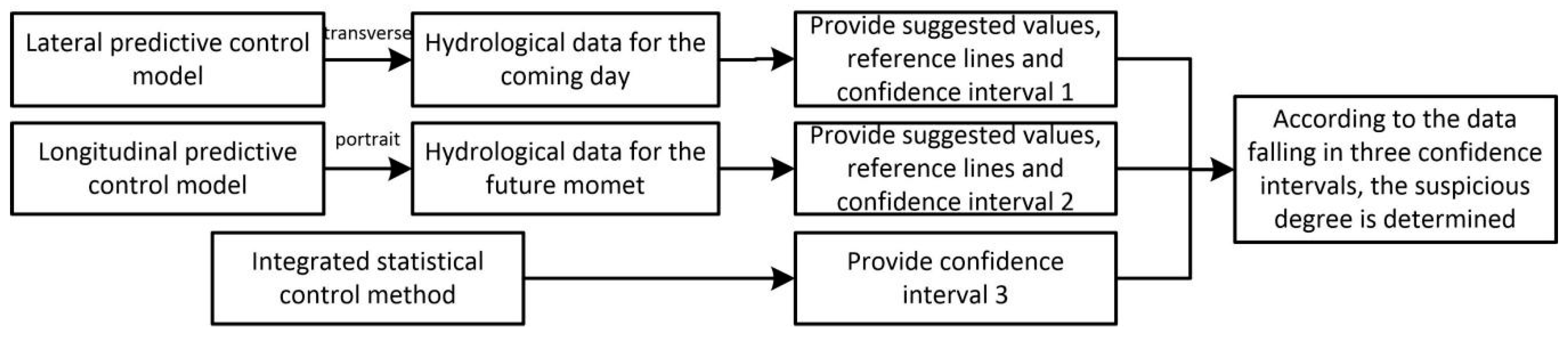
For the quality control of continuous hydrological time series, an integrated quality control scheme combining predictive control and statistical control is proposed in this paper. It includes the horizontal predictive control model, the longitudinal predictive control model, and the statistical control method based on wavelet analysis. The first two methods provide predictive reference lines and set predictive control intervals, according to predictive errors. The statistical method sets confidence intervals for real-time data, according to data consistency. If the data points are located in three control intervals, it is normal data. Otherwise, the number of control intervals violated will judge the suspicious data and the wrong data and a more credible alternative value will be provided for hydrologists instead of the suspicious and wrong data. The continuous hydrological data control method is shown in the following Figure 2.
3.1. Horizontal Predictive Control Model
Continuous hydrological time series data (such as water level and flow) have continuity and periodicity in a certain period. For continuous hydrological data, the data at the same times in adjacent two days are changed in a certain range generally. It is feasible to predict the hydrological condition of the same time in the future by using the data of the same time in history.
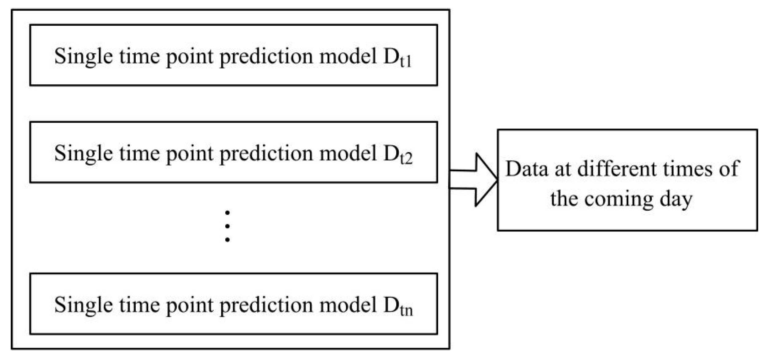
The hydrological real-time data is divided into hourly and minute levels, according to the reported time interval. The horizontal predictive control model is based on the real-time data per hour. It uses the real-time data at the same historical time to establish 24 unit control models for the next 24 h. That is, hydrologists can have a full understanding of the data changes in the coming day, according to the integrated control model (Figure 3).
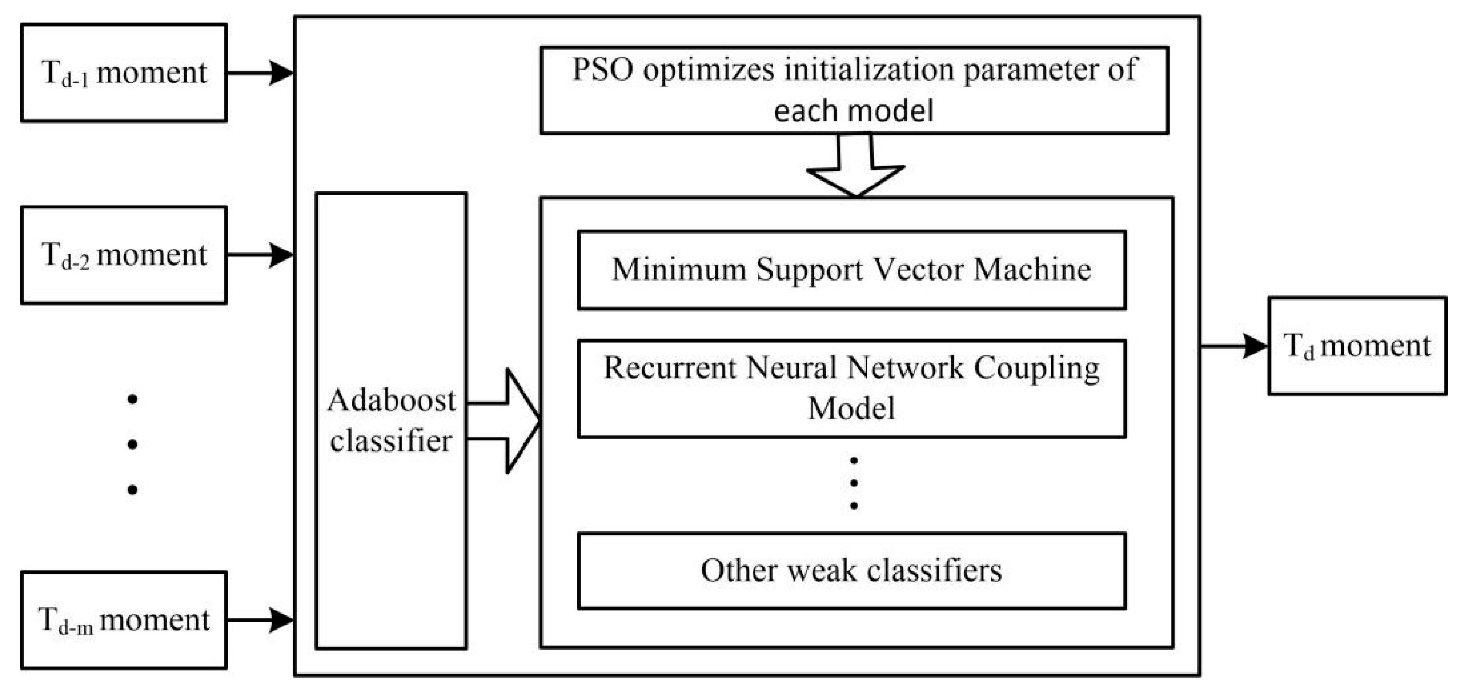
The horizontal predictive control model adopts the prediction model based on particle swarm optimization as the weak predictor and then combines several excellent weak predictors by the Adaboost algorithm to form a strong predictor. Compared with the single prediction model, the integrated predictive model has higher stability and robustness.
Particle swarm optimization (PSO) and the genetic algorithm (GA) belong to the global optimization evolutionary algorithm and both algorithms are widely used. The GA algorithm needs to adjust more parameters and is difficult to adjust. Compared with the PSO algorithm, which can solve complex nonlinear problems, the PSO algorithm needs to adjust fewer parameters and is easy to implement. Moreover, some studies [24,25,26,27] verify that the improved PSO is better than GA in optimizing the prediction model. Both recurrent neural networks (RNN) and support vector machines (SVM) are excellent predictive models and are all based on the selection of good initial parameters and high quality data. RNN is a popular learning method in the field of deep learning in recent years. Compared with the independent characteristics of the calculation results of ordinary neural networks, RNN can use its internal memory to process the input sequence of arbitrary time series, which has stronger dynamic behavior and computational ability. SVM transfers the inseparable problem in low-dimensional space to high-dimensional space to make the problem solvable. It is based on the Vapnik-Chervonenkis Dimension theory of statistical learning theory and the principle of structural risk minimization. Therefore, it can effectively avoid local minima and over-learning. If the two models are applied to the real-time control of hydrological data of automatic stations, the optimization algorithm is needed to optimize the initial parameters and select the appropriate model parameters. Using PSO to optimize the two models and select the global optimal parameters as the initial parameters of the prediction model can improve the prediction accuracy. Therefore, the real-time monitoring of the automatic station can be trained and applied without a manual selection of parameters.
The weak predictor in the Adaboost algorithm is an unstable predictive model (such as a neural network) or a variety of different predictive models. RNN is an unstable prediction model because the weights of each training network are different. Compared with the neural network, the generalization ability of SVM is stronger and the training results for the same data are stable. Selecting the single support vector machine and multiple recurrent neural networks as Adaboost weak predictors can complement the shortcomings between the algorithms and improve their generalization ability through the weighted combination of weak predictors. The SVM with larger generalization ability will be given larger weight.
An integrated predictive control model (as shown in Figure 4) is constructed for the same time in the future by using the strong predictor combined with the Adaboost algorithm. The confidence interval is established between the predicted value of the predictor and the weighted value of the mean square error to detect the reliability of the real-time data.
The horizontal predictive control model algorithm process is described below.
- Select data and normalize it to make data between (−1, 1).
- The initial parameters of SVM and RNN are optimized by PSO. The optimal SVM weak prediction model and WNN weak prediction model are established.
- Select m RNN and the best SVM. Then the m + 1 excellent models are selected as the weak predictor of Adaboost and establish the strong predictor of Adaboost.
- Referring to the predicted value and mean square error of the prediction model, the confidence interval of quality control is established with the predicted value as the center. Then the interval is connected and the upper and lower confidence intervals are smoothed by a wavelet transformation (More algorithm details can be found in the Supplementary Materials).
For the sample data, it is necessary to normalize the data so that the data is distributed between (−1, 1), which makes the sample data evenly distributed and reduces the possibility of early saturation of the weak predictor of RNN. The formula is as follows: , is the mean of all sample data and is the standard deviation of all sample data.
For the test sample data, we need to select the historical data of the same period to test and get the error standard of the strong predictor. The error of the strong predictor is related to the quality control range of real-time data. Because the hydrological data have annual periodicity, it is necessary to test the generalization ability of the strong predictor by using the hydrological data of the same historical period to make the control interval meaningful. In this way, the quality control interval of real-time data will change constantly, according to the time. For example, when the winter data changes slowly and the error is low, then the winter confidence interval will become smaller. The summer data fluctuations are larger and, therefore, its confidence interval will become larger. This dynamic adjustment of the confidence interval can improve the practicability of the control model.
The Adaboost algorithm is used to form a strong predictor to predict the real-time data simultaneously in the future and the predicted value yc and the mean square error mse are used to form a confidence interval where is a weighted value, and [27]. The confidence interval becomes when . The horizontal predictive control model is established to predict and control the data in the coming day. If the confidence interval is obtained, , . In the 24 models, there may be some abnormal predictive situations, which make some values of the confidence interval of predictive control abnormal. Common deionizing methods are easy to use to remove useful signals. Compared with common methods, wavelet analysis can use different soft and hard thresholds for the scale wave and every detail wave and maintain useful signals effectively. Therefore, the upper and lower bounds of the confidence interval are smoothed by wavelet analysis to make the adjacent control interval more consistent with the characteristics of the hour hydrological data.
3.2. Longitudinal Predictive Control Model
The hydrological real-time control station uploads m data every day with real-time characteristics. The offline training single predictive control model may cause the prediction error to increase because of the imperfect training, which makes the data predictive control deviation. However, the accuracy of the data needs real-time detection and control.
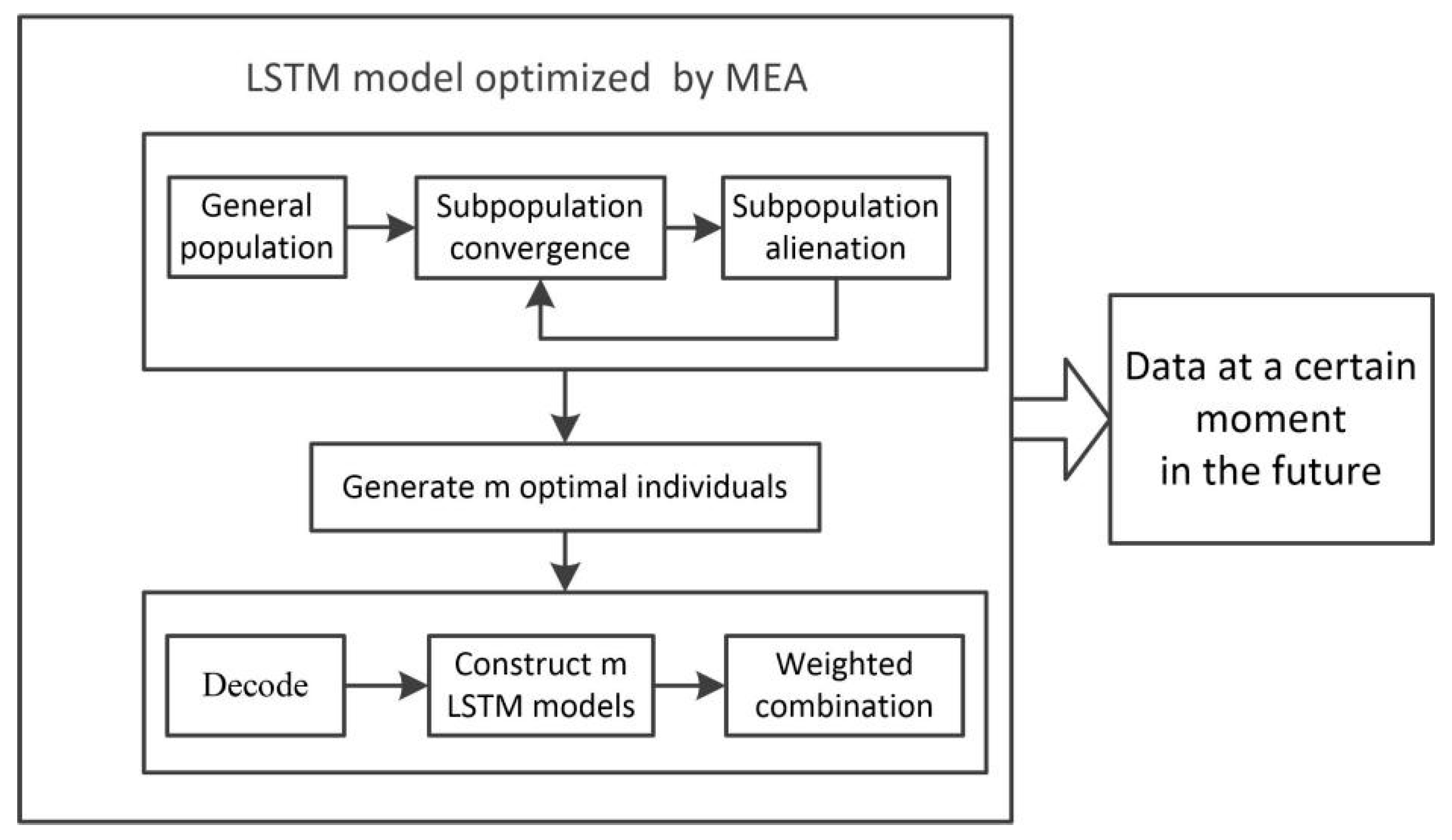
Based on the convergence and alienation of thought evolutionary algorithms and the idea of posting excellent individuals on the bulletin board, this paper improves the long-term and short-term memory network prediction model and proposes a longitudinal predictive control model. The model establishes a weighted combined control model to increase the robustness of the predictive control by selecting the first m excellent parameters on the bulletin board as the initial parameters of the network. It mainly trains the temporary model on the bulletin board after a period by using real-time historical data as the data set. If the best model in the temporary model is better than the worst model in the combined control model, it will be replaced in time. Lastly, it will be re-weighted to form the predictive control model, according to the predictive error (Figure 5).
The longitudinal predictive control model uses the temporary model to replace the worst model. In the case of ensuring that the stability of the combined model is small, the old network is replaced by a new excellent network. This method can continuously adjust the timeliness of the control model. According to the idea of MEA, the longitudinal predictive control model is constructed. The specific algorithm process is as follows.
- Training set / test set generation: Select data and normalize it to make data between (−1, 1). Then organize the data and predict the hydrological situation in the future by using the data of the previous N hours. Lastly, we randomly disrupt the sequence and select 80% of the data as the training set and the rest as the test set.
- Population generation: The initial population is randomly generated and ranked according to the mean square error from small to large. The first m individuals were selected as the center of the superior subpopulation, the first m + 1 to m + k individuals were selected as the center of the temporary subpopulation, and then m new subpopulations were generated, which surround the m centers within limits.
- Sub-population convergence operation: Convergence operation is to change the central point of the subpopulation by iteration and then randomly generate multiple points around the center to form a new subpopulation until the central point position does not change any more and the average error of the prediction model is minimized (that is, the highest score). Then the subpopulation reaches maturity. Lastly, the score of the center position is taken as the score of this sub-population.
- Subpopulation alienation operation: The scores of the mature subpopulations are ranked from large to small and the superior subgroups are replaced by the temporary subgroups with high scores. The temporary subgroups are supplemented to ensure the quantity is unchanged.
- Output the current iterative best individual and score: Find the highest scored individual from the winner subgroup as the best individual and score currently obtained and save it in the temporary array temp_best
- Select excellent individuals: The loop iteratively performs the convergence and dissimilation operations of the sub-populations until the loop stop condition is satisfied, that is, the optimal individual position does not change or the number of loop iterations is reached. Sort the array temp_best from large to small and select the top m as excellent individuals.
- Establish LSTM model: Decode m excellent individuals generated in 6, establish m LSTM models, assign the optimized initial weights and thresholds to different network models, and train the sample sets again to construct m LSTM models.
- Establish longitudinal predictive control model: use the test set to simulate the m model and then weigh the combination of m models according to the test mean square error to establish the longitudinal predictive control model.
After the above eight steps, the longitudinal predictive control model is established. Then, at intervals, m excellent individuals are selected from temp_best and k individuals randomly generated are added to form the center of the initial population and m + k populations are generated. Then perform steps 3 to 6. Lastly, the newly generated optimal individual in step 6 is selected, the optimal initialization parameter is assigned to the new LSTM model, the network is trained, and the mean square error of the new test set is obtained. If the error of the new network is smaller than the network in the combined model, use it to replace the largest error in the combined model and rebuild the combined model. Otherwise, the original combined model is not changed.
According to the data at different times, a time series curve is drawn. The predicted value at each moment on the prediction curve plus the positive and negative error values of the 95% confidence interval demarcation point of the single model prediction error is used as the upper and lower bounds of the point data control. Lastly, the control boundary is smoothed by the wavelet transformation and the part between the two smooth curves is used as the confidence interval.
3.3. Statistical Data Quality Control Model
The traditional data quality control method mainly relies on statistical methods to consistently detect and mark abnormal data and erroneous data. The test results are for expert reference.
The hydrological time series statistical data quality control method draws on the Fourier transform-based control method of Sciuto et al. [28] to establish a confidence interval by setting a fixed-size sliding window. In order to overcome the defects of the Fourier transformation, this paper uses the multi-scale refinement wavelet analysis of finite-width basis function to smooth the data of the sliding window and then the weighted mean and mean square error are obtained based on the method of giving high weights to adjacent values. The weighted mean and δ-fold mean square error are used to form a time series confidence interval to control the data quality in real time. The process flow is shown in Figure 6.
The statistical data quality control method (SDQC) is to establish a statistical confidence interval by weighted combination of horizontal and vertical statistical control methods. The algorithm steps are as follows:
- Parameter setting: Set the size of the horizontal and vertical sliding windows to n and m, respectively. The wavelet base of the wavelet analysis is the bior and the decomposition scale is k. The smoothing time span is d and the dynamic weight is and .
- Time series smoothing: The wavelet analysis is used to decompose and reconstruct the hydrological data and the smoothing sequence is obtained to reduce the short-term fluctuation and noise of the hydrological data.
- Confidence interval of hydrological time series: Taking hour real-time data as an example, the weighted mean value and the mean square error of sliding window length n at each time are obtained. Set as the confidence interval at the same time for the next day. The upper and lower bounds of confidence intervals are connected to form two upper and lower bound sequences and then the two sequences are smoothed by wavelet analysis to eliminate possible mutation points. If the interval change rate is large, the range of the error rate is limited to reduce the interval cell variation rate.
- Confidence interval of longitudinal time series: The monitoring data of the first m times are smoothed by wavelet analysis and the weighted mean value and mean square error are obtained. In addition, set as the confidence interval of real-time data at the next time, which needs to be constantly adjusted.
- Comprehensive confidence interval: The weighted control interval is obtained by using the confidence interval of the vertical time series and the horizontal time series at the same time.
3.4. Continuous Hydrological Data Quality Control Method
The continuous hydrological data quality control method combines the above two consistency check prediction control models and adds regular QC methods in meteorological fields such as the format check, lack of test, the extreme value check, and the time-varying check to carry out comprehensive quality control for hydrological data.
The continuous hydrological data quality control method consists of four parts: missing inspection, format inspection, extreme value inspection, and consistency inspection. The missing inspection is to detect data points that cannot be uploaded due to instrument failure. The format inspection is to check the date of the real time uploading system and whether the format of the station code conforms to the specification. Climate extreme value inspection is to detect the quality of real-time data uploaded from stations. Climate extreme value depends on the extreme value of regional historical data. If the real time data is greater than the extreme value, it is labeled as the wrong data. The consistency check is divided into two consistency checks: time and space. The temporal consistency includes the time-varying checking of the detection elements and the changing relationship between the multi-elements of the same station (such as the relationship between the water level and the discharge of the station). The spatial consistency is checking and controlling the consistency by using the correlation of the elements between the regional stations.
Continuous hydrological data quality control method establishes three confidence intervals with two predictive control methods and statistical data quality control methods on the premise of basic QC inspection. If the hydrological real-time data is in three confidence intervals, the data is considered to be correct. Otherwise, it is considered suspicious. According to the number of confidence intervals of data violation, the suspicious degree is formulated into three grades. In addition, there are six grades in all.
- Level 1: Data is outside a confidence interval.
- Level 2: Data is outside two confidence intervals.
- Level 3: Data is outside all confidence intervals.
- Level 4: Data is larger than the time varying rate.
- Level 5: Data is outside the maximum and minimum value.
- Level 6: The missing and malformed data.
As the number of intervals in which the detected data is violated increases, the suspiciousness of the data increases. All suspicious data, the erroneous data, and the missing data of the basic control detection are recorded in the system log and the recommended value of the real-time data modification and its credibility are given by the predictive control model, which can be referred by the water supply staff.
In the quality control process, if the data is missing, the horizontal predictive control model is used to give a suggested value and the input of the longitudinal predictive control model is replaced by the former recommended value. The statistical confidence interval is the horizontal time series confidence interval. This ensures that, in the event of an instrumental failure, it can still supply hydrological staff the three confidence intervals and recommended values of the real-time data for reference. If the lack of measurement time is long, the hydrological data of the adjacent station is required to help fill the measurement time.
4. Discrete Hydrological Data Control Model
The discrete hydrological data control model is aimed at hydrological data with large spatial and temporal differences such as rainfall. It uses spatial correlation of adjacent stations to establish network weight topology and dynamically adjusts network weight value according to real-time data correlation between stations in order to provide reference for hydrological workers to fill in the data. The data of automatic measurement stations with larger weights around the stations are selected for spatial interpolation. The advantages and disadvantages of the spatial interpolation method are analyzed by fitting error and the suitable method is found to detect and control the discrete data. The flow chart is shown below (Figure 7).
4.1. Hydrological Spatial Topological Structure
Among the hydrological data elements, the rainfall is not easy to control and test the data due to the large spatial anisotropy and poor time continuity. The method of controlling and checking the data of the rain gauge station through single station consistency does not work and spatial consistency data quality control between multiple stations is required. It makes use of the spatial distribution characteristics of hydrological elements and the distance, altitude, and topography between the regional hydrological automatic stations as well as the correlation degree between the elements and space affect the control effect.
In order to let hydrologists understand the relationship between an automatic station and other stations around it, this paper establishes a weight map of the station relationship based on the location and rainfall data of the automatic station so that hydrologists can understand the relationship between the stations in the whole basin or region. The construction of a regional topology network requires the following steps.
- Screening stations: Taking the measured stations as the center, the peripheral stations with radius distance S as the candidate set n are selected and marked, and then the station m with sufficient hydrological data are selected from the candidate stations.
- Constructing time series: Extracting the station data set in the specified time from the compiled historical hydrological database and counting the monthly factor values and constructing the m monthly time series.
- Correlation analysis: Analyze the correlation coefficient between the station under test and the m surrounding stations and obtain the correlation coefficient set between m + 1 stations where . The correlation coefficient set of the station under test is sorted from large to small and the stations with large correlations are selected (the general coefficient is above 0.6).
- Preserving the correlation coefficient: The station code and the coefficient, which have the bigger correlation coefficient with the station under test, are saved in the station relation table st-relation. In addition, for the other m stations, the stations with correlation coefficients greater than 0.6 are selected and stored in the table st-relation.
- Constructing regional networks: Looping steps 1 to 4 and constructing relational networks. The difference is that only unmarked peripheral stations are selected in step 1, which can greatly reduce the construction time of the regional station network.
First, in the construction of the station network, choosing the historical hydrological data as the data set of the model can reduce the influence of a large number of abnormal or erroneous data and make the network model coincide with the actual relationship. Second, for the hydrological elements with poor continuity such as precipitation, the time series composed of monthly precipitation with a large grain size is selected to calculate and construct the relationship network between stations. Because the time series consisting of daily, hourly, or minute precipitation has a small particle size, the missing or abnormal data have a great influence on the time series. For example, the correlation coefficients of monthly grain size of Shangli rainfall station with Chishan and Pingxiang rainfall stations on Xiangjiang River in Jiangxi Province are 0.85 and 0.77, respectively, while those of daily grain sizes are 0.78 and 0.73, respectively, and those of hourly grain sizes are 0.72 and 0.68, respectively. Lastly, the markup method is used to avoid repeated modeling and reduce the time of establishing the whole network.
Taking the radius S of the measured stations as a reference, the closeness of the stations is defined by the correlation coefficient between the data of the hydrological stations and the correlation network of the regional hydrological stations under the specified factors is constructed. Hydrologists can refer to the similarity coefficients between the measured stations and the surrounding stations and rely on the hydrological conditions of the surrounding stations to fill in missing or suspicious data in order to provide a basis for filling and replacing the hydrological data.
4.2. Dynamic Adjustment of the Topological Structure
For the correlation between hydrological stations considered as a whole above, the correlation of data between regional stations varies when applied to a particular season or month (as shown in Table 1).
It can be seen from the table that the overall correlation coefficients of Shangli with Chishan, Pingxiang, and Zongli rainfall stations on the Xiangjiang River in Jiangxi Province are 0.85, 0.77, and 0.56, respectively, while the correlation coefficients of spring, summer, autumn, and winter have some changes with the overall coefficient. For example, the correlation coefficient between Laoguan and Shangli in the spring is small while the other three seasons are relatively large. The correlation coefficient between Zongli and Shangli in the autumn and the winter is small and the correlation coefficient between the four stations and Shangli in the summertime is relatively low. Then, if only the overall correlation coefficient is used as a reference, it will result in an inability to accurately reflect the true correlation in different periods.
The correlation coefficients of the factors between stations will change with time and the correlation coefficients are directly related to the reliability of the data. Therefore, reducing errors and suspicious data can increase the confidence of the correlation coefficients. The variation of hydrological station elements is seasonal and periodic and the dynamic adjustment of the topological structure of the elements will provide a better basis for the hydrological workers to fill in the missing data and replace the suspicious data.
4.3. Spatial Interpolation Model
Influenced by the range and density of precipitation, the precipitation will form different rainfall grading lines in space. The spatial difference makes the area and direction of each precipitation process different, which will make the real-time rainfall difficult to control. Therefore, the basic QC detection method (time-varying rate test) is used to detect and control the hourly or minute rainfall while the spatial interpolation method is used to check the statistical daily rainfall data and the coarse-grained control of the quality of rainfall data is reliable.
Based on the correlation coefficients of the stations under test, a variety of spatial interpolation methods (such as Inverse Distance Weight, the Trend Surface Method, and the Kriging Method) can be constructed quickly. The multivariate SVM model and the commonly used spatial interpolation methods are constructed to compare. The input terms of various spatial interpolation methods and multivariate SVM models are the regional station data with the same elements at the same time as the station being measured and the outputs are the values of the measured stations at the same time.
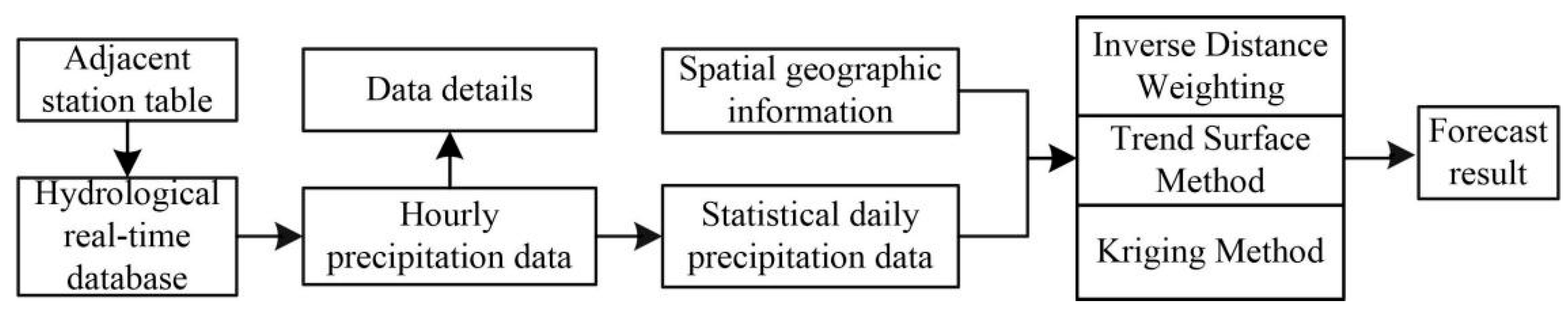
The specific process is shown in Figure 8.
The construction of the spatial quality control model is divided into the following steps:
- Referring to the table information of adjacent stations, the hourly real-time rainfall data of selected adjacent stations are extracted from the hydrological real-time database.
- View the data details and count the daily precipitation data without missing stations on the day.
- Using spatial geographic information (such as longitude and latitude or elevation) and daily precipitation data to construct three spatial interpolation methods, these three spatial interpolation methods have nothing to do with historical data. The model parameters are changed with the changes of regional data.
- Establish a three-dimensional space model and obtain predicted results based on the geographic information of the stations.
In order to improve the prediction accuracy of the spatial interpolation method, the spatial interpolation method is constructed by using the stations with large correlation coefficients in the same period (quarterly).
The final form of constructing the model by spatial interpolation is to assign a weight value to the stations around the region, which belongs to linear interpolation. In view of the uncertainty of rainfall data, the method of establishing the spatial prediction model only by using rainfall data of peripheral stations with coordinates is a little inadequate. Therefore, the suspicious data detected by the spatial interpolation method needs to be further checked and confirmed by manual intervention.
4.4. Discrete Hydrological Data Quality Control Method
The discrete hydrological data quality control method is mainly for the quality detection and manual replacement of hydrological elements (such as rainfall) with large spatial, temporal differences and strong spatial correlation. The steps are shown below.
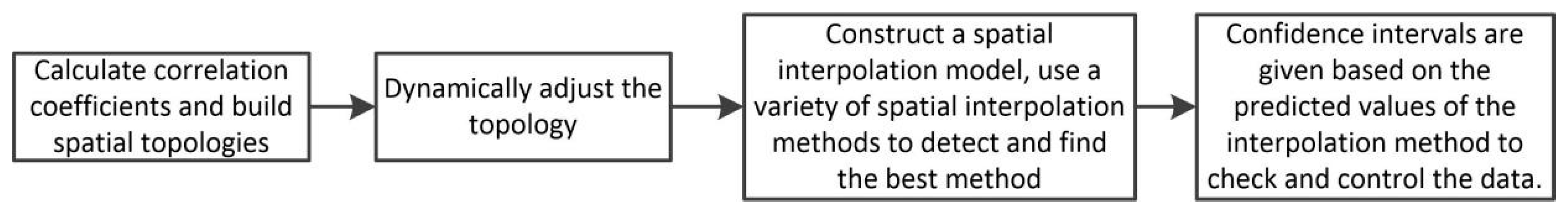
- Calculate the correlation between the station under test and the surrounding stations based on the spatial geography and data association of hydrological elements and construct a spatial topology.
- The correlation will change with the change of seasons. It is necessary to dynamically adjust the topology to fill the reference data and suspicious data for hydrological workers.
- Construct a spatial interpolation model, use a variety of spatial interpolation methods to detect spatial consistency, compare various linear spatial interpolation methods with nonlinear multivariate SVM methods, and analyze their advantages and disadvantages.
- Based on the predicted value of best-improved inverse distance spatial interpolation method, the confidence interval is given to check and control the daily precipitation data.
5. Experimental Analysis
5.1. Experimental Analysis of Continuous Data
Data preparation: The real-time data of the water level of the Guxiandu station on the Rao River in Jiangxi Province was used in the experiment. The time is recorded once every hour from 1 January 2006 to 31 December 2011, which is a total of 52,558 records. The sample data from 2006 to 2010 was selected as the training set and the 2011 sample data was used as the test set.
5.1.1. Experimental Analysis of the Horizontal Predictive Control Model
The horizontal predictive control model is to model 24 time points separately. Therefore, 24 predictive models need to be established to predict and control the data of the next day. The data is classified by the punctual time and 24 data sets are obtained in which each is 2190 records. The sample data from 2006 to 2010 was selected as the training set and the 2011 sample data was used as the test set.
When filling in the missing data and suspicious data, it is necessary to give the staff more accurate predictive value for reference and replace the original data with the predictive value. The following is a comparative analysis of the stability and prediction errors of the horizontal predictive control model (HPCM), the BP neural network, the RNN model, and the SVR model.
Figure 9 shows the water level value predicted by various models from 1 May 2011 to 8 May 2011 at 8 a.m. It is found that the horizontal predictive control model is better than other models and the error is relatively small. In the figure, we can also find that the overall error of SVR and RNN is smaller than that of the BP neural network. At the same time, SVR is slightly more stable than RNN. This indirectly shows that the combination of RNN and SVM is effective for HPCM and it is reasonable to give SVM, which has similar ideas with SVR high weight. The robustness (stability) of each model is analyzed below (Figure 10).
Figure 10 shows the rmse of the water level data at 8 a.m. in 2011. As can be seen from Figure 10, the rmse of the horizontal predictive control model is between (0.275, 0.289), the rmse of the BP neural network model is between (0.281, 0.366), the rmse of RNN model is between (0.289, 0.301), the rmse of SVR model is between (0.282, 0.298). It can be seen that the BP neural network is the most unstable while other models are relatively stable. The fluctuation of SVR is smaller than that of RNN because the generalization ability of SVR is stronger and more stable. Among them, the HPCM fluctuates less with the training data while its rmse is smaller. This may be because HPCM combines SVM and RNN, which has stronger generalization ability as well as the smallest fluctuation and relatively smaller rmse. This indicates that HPCM is very stable.
5.1.2. Experimental Analysis of the Longitudinal Predictive Control Model
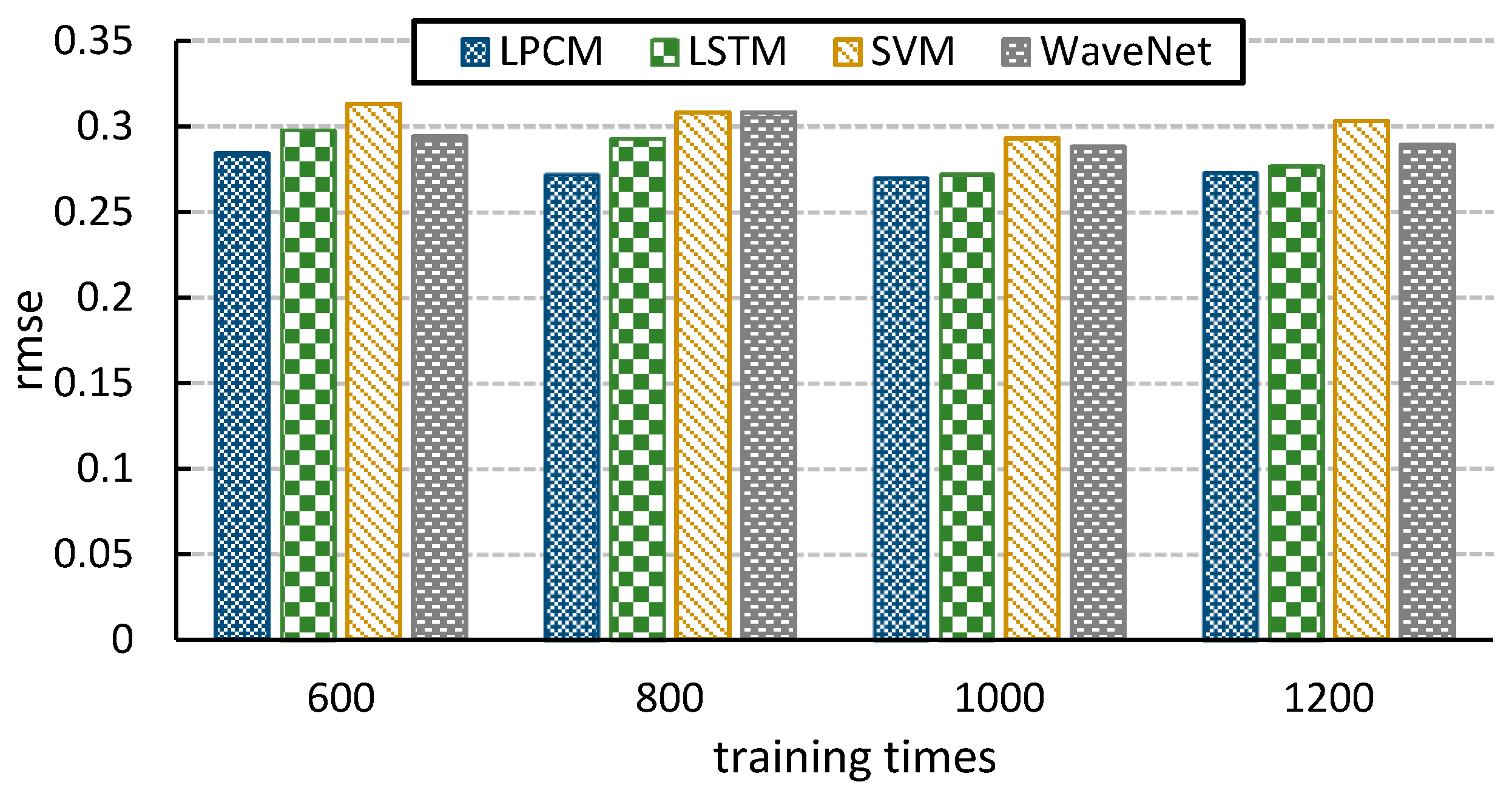
Since the water level change at 24 h a day is generally not very large, the error analysis here uses the predicted value at 8:00 a.m. from 1 October 2011 to 7 October 2011. The following is a comparative analysis of the stability and prediction errors of the four models of the longitudinal predictive control model (LPCM), the LSTM model, the SVM model, and the newly proposed WaveNet model [29].
The main component of the Wavenet model is a causal, dilated convolution network. Each convolution layer convolves the previous layer. As the convolution kernel increases, the number of layers increases and the perception in the time domain is stronger and the receptive field is even larger. Wavenet combines causal convolution and dilated convolution to allow the receptive field to multiply as the depth of the model increases. The increase in the receptive field is very important for long-term dependence in the construction of hydrological time series models.
Figure 11 shows the predicted value of different models at 8 a.m. from 1 October 2011 to 8 October 2011. In Figure 12, it is found that the longitudinal predictive control model is better than the other models and the error is relatively small. As a typical model in deep learning, the LSTM model is better than the SVM model. Even though the local error in LSTM may be a little larger than WaveNet, the overall error is smaller than in the WaveNet model. This indirectly shows that, in the longitudinal predictive control model, using LSTM to combine the model is better than using other models. The robustness (stability) of each model is analyzed below (see Figure 12).
As can be seen from Figure 12, the rmse of the longitudinal predictive control model is between (0.270, 0.284), the rmse of the LSTM model is between (0.272, 0.298), the rmse of the SVM model is between (0.293, 0.313), and the rmse of the WaveNet model is between (0.288, 0.308). In all models, the longitudinal predictive control model fluctuates less with the training data and the rmse is smaller. LSTM is better than SVM and WaveNet. Therefore, LPCM uses LSTM to optimize and uses good models to replace the poor model prediction results in combination to make the effect of LPSM better. This indicates that the stability of the longitudinal predictive control model is better.
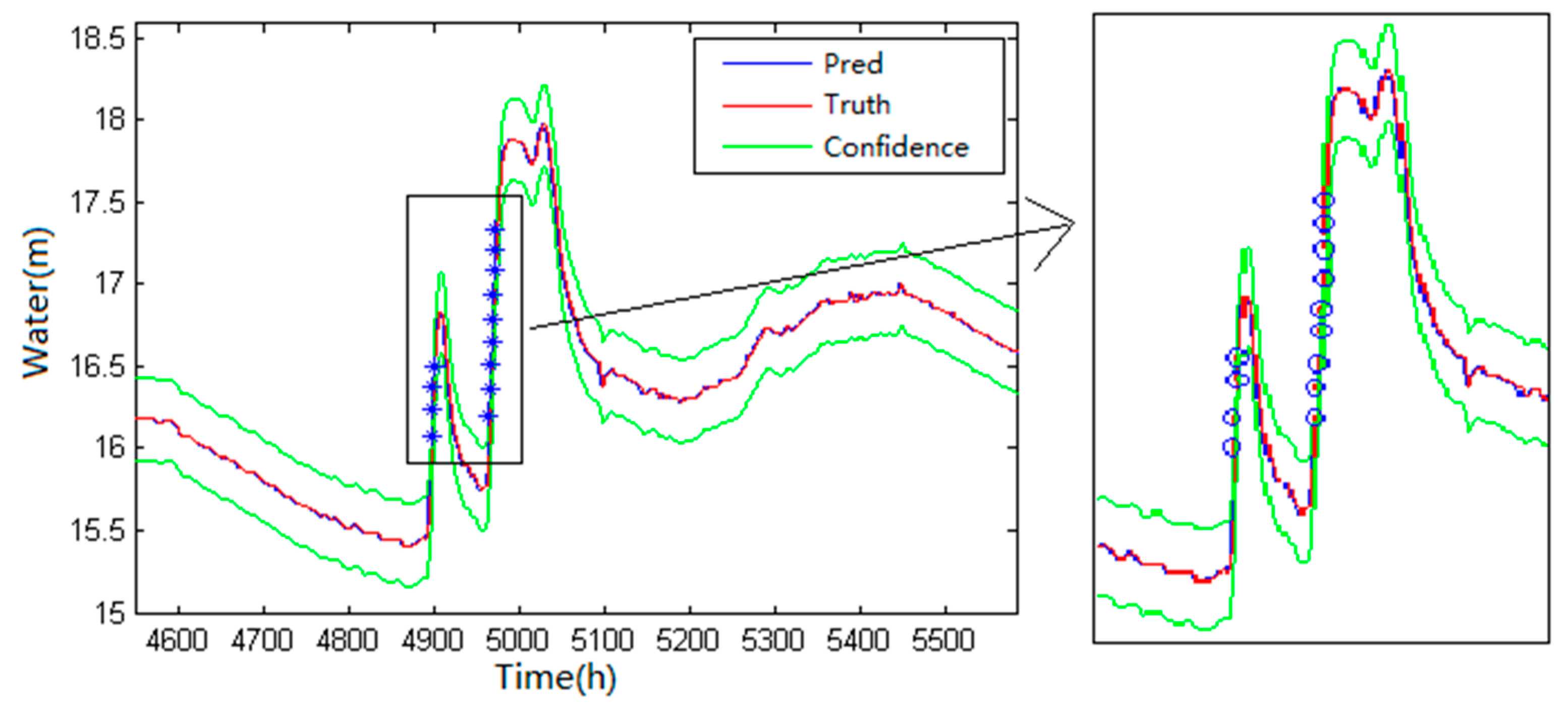
Figure 13 shows the control effect of the longitudinal predictive control model in the flood season of Guxiandu Station. The red line represents the predicted value, the blue line represents the actual value (or monitoring value), the two green lines are confidence intervals, and the blue stars are the detected abnormal data.
Analysis of the actual value and the predicted value of the graphics found that because the correlation coefficient between the hourly real-time data is large, the predicted value and the actual monitoring value of the longitudinal predictive control model fitting effect is very good. During the five days period from 4900 to 5000, the water level rapidly increased, declined, and then increased. There may be a heavy rain during these times or a large amount of water from the upper reaches came here. Due to the rapid change of water level, the data in these two periods are outside the confidence interval and are classified as suspicious periods, which need to be identified by hydrologists.
5.1.3. Experimental Analysis of the Statistical Data Quality Control Model
Figure 14 shows the effect of the comprehensive statistical quality control process during the flood season at the Guxiandu Station. The red line represents the average value, the blue line represents the actual value (or monitoring value) and the two green lines are confidence intervals.
As can be seen from Figure 14a, the statistic control method can construct a stable control interval for the stable region and the normal monitoring value is in the middle of it. It was found that the average value of the historical data window has lag compared with the actual detection value, which is the disadvantage of the statistical control. In positions 2580 to 2650, the rapid change of data results in large fluctuations in the upper and lower bounds of confidence intervals during this period. The statistical control interval is changed with the change of data size. The rapid change of the confidence interval does not meet the actual needs of hydrological data control.
Figure 14b shows the statistical control method in this paper. It is found that the lag and the interval change rate has been reduced. This is because the weighted average is used to establish confidence intervals and limit the rate of error variation in the improved statistical control method. From the figure, we can see that the statistical control effect of the method in this paper meets the actual demand.
5.1.4. Experimental Analysis of Continuous Hydrological Data Control
The continuous hydrological data control method (CHDC) was used to control the data of 72 months from 2006 to 2011 at the Guxiandu Water Level Station. Because the predictive control part needs training samples, we select the data from 2006 to 2010 for 60 months to train the model and control the data quality of the 12 months in 2011.
Table 2 shows the number of anomalies detected by different methods. All methods have undergone missing detection, extremum detection, and time-varying detection. Experiments show that the method proposed in this paper can detect suspicious values better. The single HPCM, LPCM, and statistical methods can detect many suspicious values, but they can be better combined to find all the suspicious values (More result details can be found in the Supplementary Materials).
5.2. Experimental Analysis of Discrete Data
5.2.1. Build Topological Structure
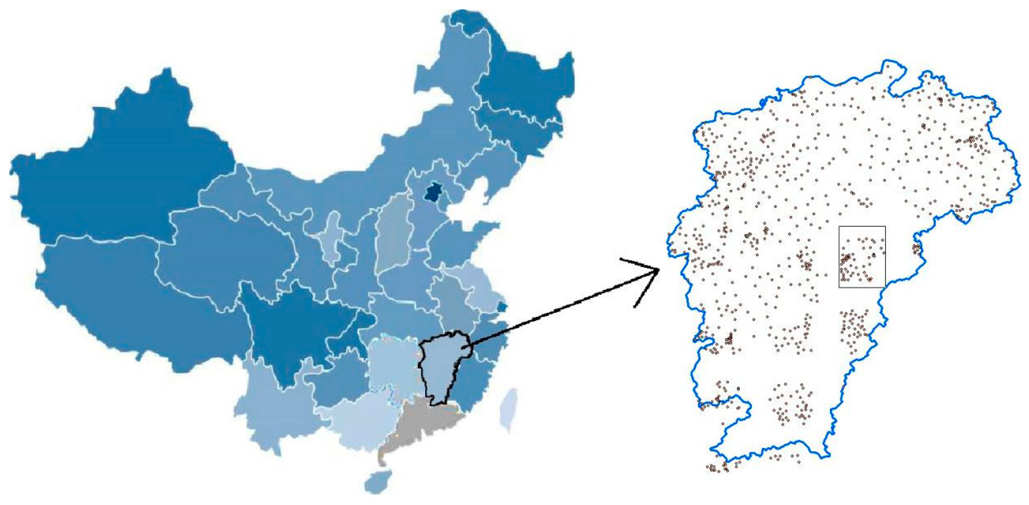
Data preparation: in this experiment, the Jiangxi Rainfall Station analyzes the spatial interpolation method. Figure 15 is the map of the Jiangxi Province. The point represents 812 rainfall stations in the Jiangxi Province. The selected part of the frame is the rainfall station for the spatial interpolation experiment.
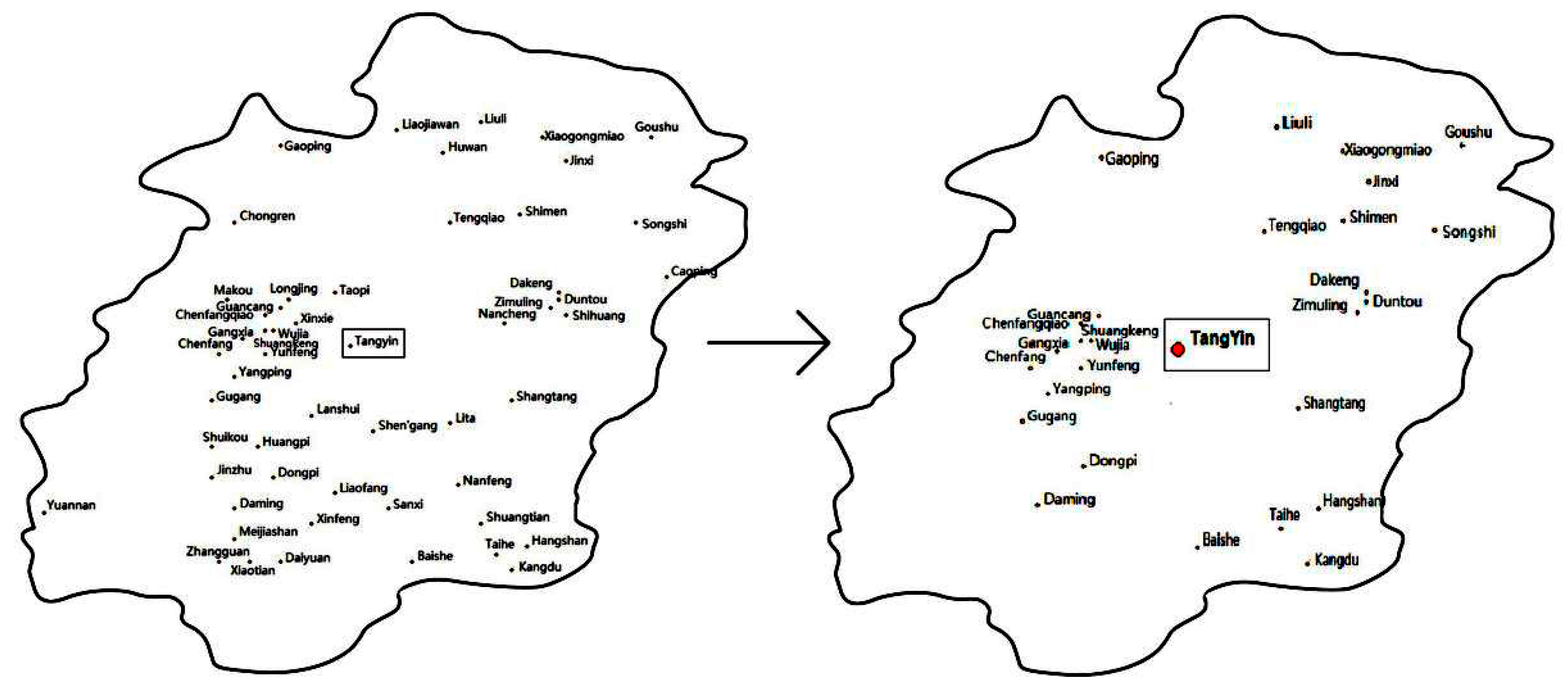
The enlargement effect of the box selection section is shown in Figure 16. The Tangyin station is located in the Fuhe River system of the Yangtze River valley. The Fuhe River system is an important branch of the Yangtze River Valley and the Poyang Lake valley. Therefore, it is meaningful to study the correlation between precipitations and ensure the quality of the data in the regional stations of the Fuhe River system.
Fifty-three rainfall stations around the location of the station are chosen as experimental objects. Due to the uncertainty of station time and data reporting of each station, some stations have been abandoned or too much data is missing. Therefore, the initial screening of the station is required before the model is built. We removed the stations with less historical data and found that 11 rainfall sites such as Daiyuan, Taopi, Xinxie, Makou, Chongren, Huwan, and so on have either been deactivated or have a large amount of missing data and need to be removed.
The daily rainfall data from 1 January 2000 to 31 December 2007 was selected as experimental data and the sum of monthly rainfall of each station was counted. The correlation between 42 stations will be calculated with the monthly rainfall of eight years. Select Tangyin station and other stations whose correlation coefficients were greater than 60% as candidate stations, which is a total of 27 stations (as shown in Figure 17).
As shown in Table 3, the horizontal distance of the candidate stations is within 50 km. Except for Yangping and Taihe, the other elevation distances are within 200 m. The correlation between rainfall data is related to the horizontal distance and the altitude distance. For example, although Shuangkeng is far from Tangyin elevation, its horizontal distance is close. Therefore, the correlation coefficient is relatively high while Kangdu is far away from Tangyin, but the altitude is only 4 m. Therefore, the correlation coefficient is relatively high too. There is also a special case such as the horizontal distance between Daming and Tong Yin, which is 24.6 km. The elevation distance is 119 m and it is large. However, the correlation with the Tangyin Rainfall Station is the highest, which may be caused by the topography of the surrounding area of the station.
5.2.2. Experimental Analysis of the Spatial Interpolation Model
In this experiment, the daily rainfall data of the Tangyin station in June 2007 was taken as an example for spatial interpolation.
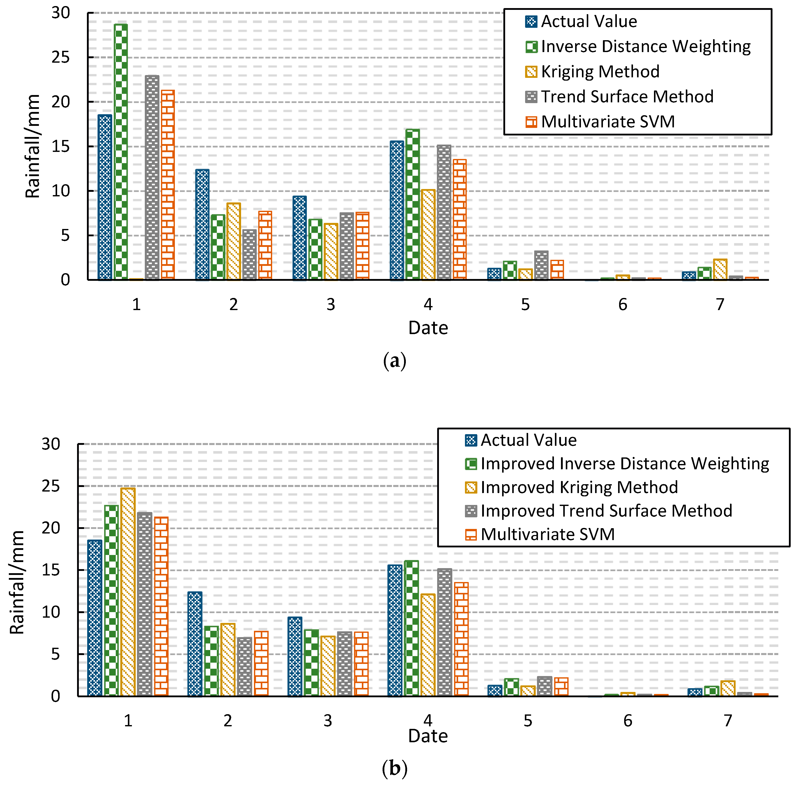
Figure 17a shows the comparison of the interpolation effects of the three spatial interpolation methods and the multivariate SVM in the period of more precipitation from 1 June 2007 to 7 June 2007. As can be seen from the figure, the errors of the three spatial interpolation models are larger than those of the multivariate SVM model. This shows that the interpolation method of plotting three-dimensional precipitation time-trend surface only by using spatial coordinates and the data of the surrounding stations at the same time is not as good as SVM constructed by using the historical data of the surrounding stations. On June 6, there was no precipitation in Tangyin. Because of the precipitation around some stations, the filled data was larger than 0. However, it was found that the maximum predicted value of the four models was generally 0.2, which is close to 0.
In Figure 17b, three improved spatial interpolation methods and multivariate SVM are used to compare the interpolation effects in the week with more precipitation from 1 June 2007 to 7 June 2007. From the table data, we can see that the error of the three spatial interpolation models constructed by the stations with a large correlation coefficient is higher than that of the original spatial interpolation method. Among them, the improved inverse distance weighting method is the most clear, which is even better than the multi-dimensional SVM. This may be because the inverse distance weighting method itself depends on the layout of the sample points and the experiment selects a station with a large correlation coefficient within a certain distance to construct the model, which improves the accuracy of the inverse distance weighting method.
In Table 4, the maximum error of the trend surface method is the smallest. The root mean square error of multivariate SVM is the smallest, the mean error is the minimum, and the prediction confidence is the largest. Multivariate SVM is the best. In order to improve the prediction accuracy of the spatial interpolation method, we construct the spatial interpolation method by using the stations with large correlation coefficients in the same period (quarterly) in the topological structure.
Table 5 shows that the improved spatial interpolation method has a slight improvement in overall error and confidence with an overall increase of 1.5%. The inverse distance weighting method has the least maximum error, the least root mean square error, the least mean error, the greatest prediction confidence, and the most obvious improvement. The results show that it is effective to construct the spatial interpolation model by finding the peripheral stations with a large correlation coefficient based on the topological structure established in this paper, which can improve the prediction accuracy of spatial interpolation.
In addition, Table 4 and Table 5 show that the maximum error of each model is more than 45 and the query discovery is the data of the Tangyin station from 20 August.
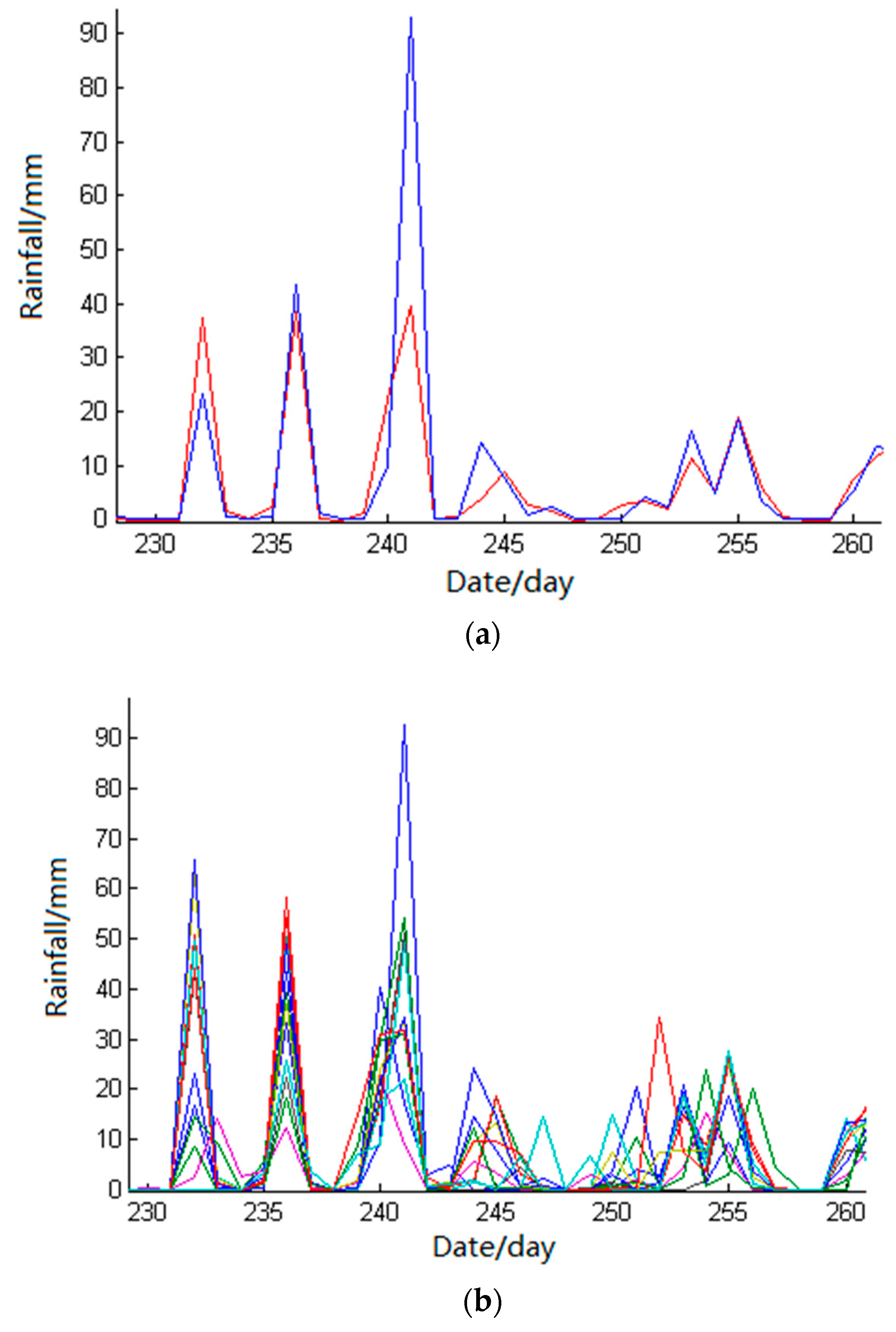
Figure 18a is a comparison chart of daily precipitation data between prediction and statistics. The blue line is the actual value and the red line is the predicted value. As can be seen from the graph, the blue line rose rapidly in 20 August.
Figure 18b is a comparison map of the surrounding stations in which the blue line represents the rainfall of the station at the station. As in Figure 18, precipitation in 20 August is much larger than that in other peripheral stations. Combining hourly precipitation data, it was found that precipitation between 5 p.m. and 7 p.m. was up to 86.7 mm. By analyzing the historical maximum of the station, it is found that the maximum daily precipitation in the rainy season reaches 157 mm, which indicates that the station is affected by extreme weather. If it follows the data quality control process, this point is determined to be an abnormal point.
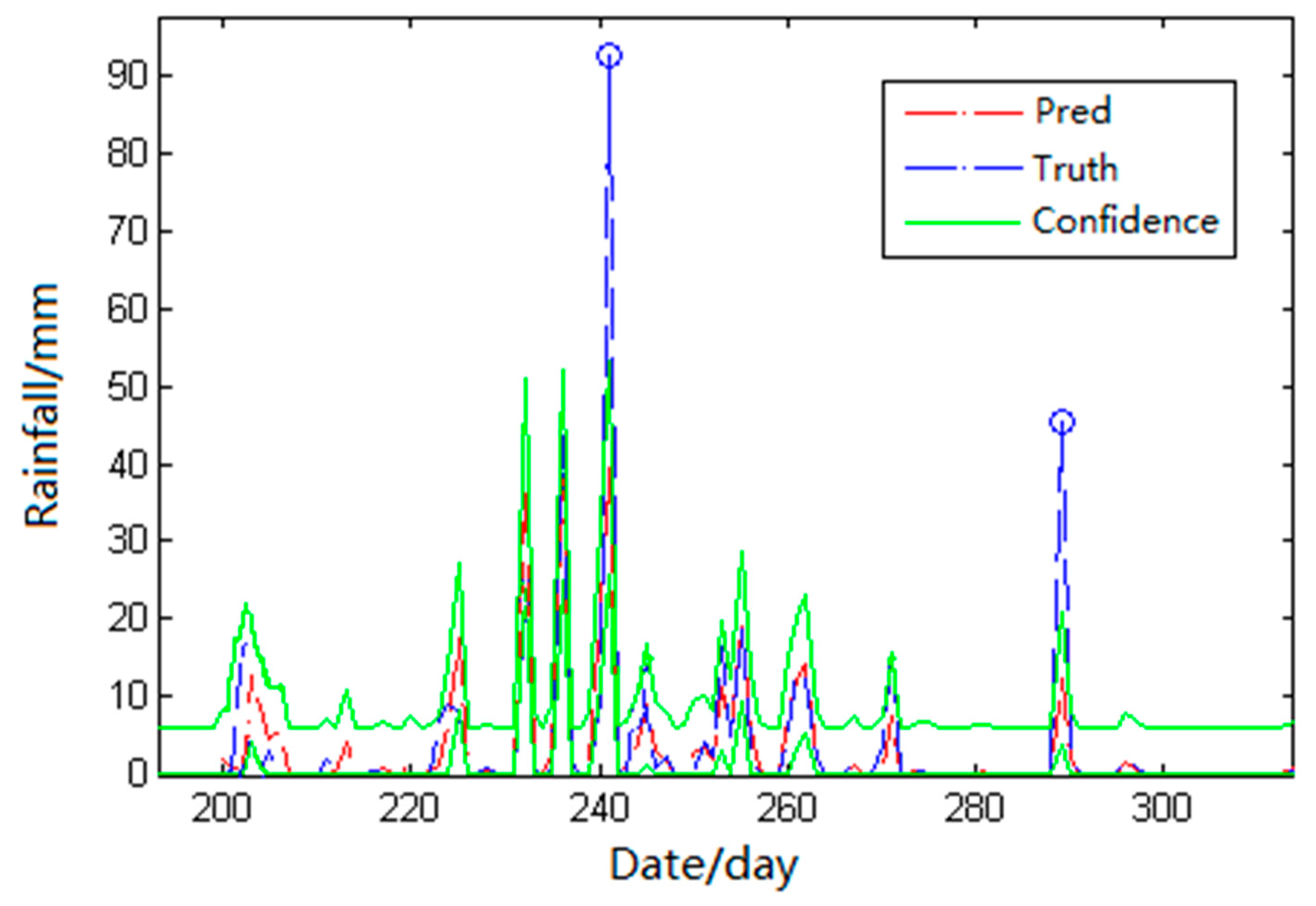
Figure 19 shows the suspicious data detection graph of the improved inverse distance weighting method. The red dotted line is the predicted value, the blue dotted line is the actual statistical value, the green solid line is the boundary of the confidence interval, and the blue circle is the detected suspicious data point.
In Figure 19, there are two suspicious data points from June to September in Tang Yin. The results of the spatial interpolation model based on simultaneous data coordinate the position and the elevation of the stations around the region, which have some improvement. More Rainfall-Related factors can be added to build the control model to improve the prediction accuracy and increase the controllability of rainfall.
6. Conclusions
According to the characteristics of hydrological data and combined with the idea of predictive control, this paper studies the methods of data quality control and data consistency and puts forward the hydrological data quality control method based on data-driven methods.
For continuous hydrological data, the method is established from the perspective of time consistency. Two combined predictive control models, one statistical control model and the corresponding control interval are constructed to detect and control the hydrological factors such as water level and discharge with good continuity from the horizontal, vertical, and statistical perspectives and the suspicion degree is set by the number of data violating the control interval. For the suspicious data and the short-term missing data, the model provides the recommended value and confidence interval.
For discrete hydrological data, the method is established from the point of view of spatial consistency. Aimed at the disadvantage that rainfall data is difficult to control, this paper constructs the topological relation diagram of correlation coefficients centered on the measured stations, studies and analyzes the advantages and disadvantages of various spatial interpolation methods, points out that the prediction effect of ordinary spatial interpolation method is poor, and finds that the spatial interpolation method based on the station data with large correlation coefficients can improve the prediction effect.
Experiments show that the proposed method can detect and control the hydrological data more effectively and provide a highly reliable substitution value for the hydrological workstation as a reference. Yet, there are still many shortcomings in this paper. For example, the network topology established in the discrete hydrological data quality control model can consider more hydrological factors (such as slope, slope direction, and the location of the station away from the water). For hydrological elements with large spatial variability (such as precipitation), more factors (such as regional seasonal periods) can be considered as auxiliary factors to construct the spatial interpolation model.
Supplementary Materials
The following are available online at https://www.mdpi.com/2073-4441/10/12/1712/s1, Figure S1: Statistical chart of data quality test results of Guxiandu station., Table S1: Abnormal check list of water level hourly data in Guxiandu station in 2011.
Author Contributions
Conceptualization, Q.Z. Methodology, Q.Z. and X.C. Software, Q.Z. and X.C. Valida, Q.Z., D.W., and Y.Z. Formal analysis, Q.Z. Investigation, X.C. and Y.Y. Resources, D.W. and Y.Z. Data curation, Q.Z. and X.C. Writing-Original draft preparation, Q.Z. Writing-Review and editing, D.W. and Y.Z. Visualization, Q.Z. and Y.Y. Supervision, D.W. and Y.Z. Project administration, D.W. and Y.Z.
Funding
This research received no external funding.
Acknowledgments
This work has been partially supported by The National Key Research and Development Program of China (Nos. 2018YFC0407900) and the Ministry of Water Resources Public Welfare Industry Research Special Foundation of China (No.201501022).
Conflicts of Interest
The authors declare no conflict of interest.
References
- Hu, G. Thoughts on the informationization of water conservancy. China Water Conserv. 2002, 11, 50–51. [Google Scholar]
- Sciuto, G.; Bonaccorso, B.; Cancelliere, A.; Rossi, G. Probabilistic quality control of daily temperature data. Int. J. Climatol. 2013, 33, 1211–1227. [Google Scholar] [CrossRef]
- Steinacker, R.; Mayer, D.; Steiner, A. Data quality control based on self-consistency. Mon. Weather Rev. 2011, 139, 3974–3991. [Google Scholar] [CrossRef]
- Sciuto, G.; Bonaccorso, B.; Cancelliere, A.; Rossi, G. Quality control of daily rainfall data with neural networks. J. Hydrol. 2009, 364, 13–22. [Google Scholar] [CrossRef]
- Abbot, J.; Marohasy, J. Application of artificial neural networks to rainfall forecasting in Queensland, Australia. Adv. Atmos. Sci. 2012, 29, 717–730. [Google Scholar] [CrossRef]
- Fu, F.; Luo, X. Study on quality control method of hydrological data. Water Resour. Inf. 2012, 5, 12–15. [Google Scholar]
- Yu, Y.; Wan, D. An application research of Bedford′s Law in hydrological data quality mining. Microelectron. Comput. 2011. [Google Scholar] [CrossRef]
- Yu, Y.; Zhang, J.; Zhu, Y.; Wan, D. Data quality control and management for hydrological database. Hydrol. 2013, 33, 65–68. [Google Scholar]
- Potter, C.; Venayagamoorthy, G.K.; Kosbar, K. RNN based MIMO channel prediction. Signal Process. 2009, 90, 440–450. [Google Scholar] [CrossRef]
- Vinayakumar, R.; Soman, K.P.; Poornachandran, P. Detecting malicious domain names using deep learning approaches at scale. J. Intell. Fuzzy Syst. 2018, 34, 1355–1367. [Google Scholar] [CrossRef]
- Ding, S.; Qi, B.; Tan, H. An overview on theory and algorithm of support vector machines. J. Univ. Electron. Sci. Technol. China 2011, 40, 2–10. [Google Scholar]
- Zhou, Y.; Huang, C.; Hu, Q.; Zhu, J.; Tang, Y. Personalized learning full-path recommendation model based on LSTM neural networks. Inf. Sci. 2018, 444. [Google Scholar] [CrossRef]
- Kennedy, J.; Eberhart, R. Particle Swarm Optimization, Proceedings of ICNN’95—International Conference on Neural Networks, Perth, WA, Australia, 27 November–1 December 1995; IEEE: Piscataway, NJ, USA, 1995. [Google Scholar]
- Chen, C.; Tian, Y.; Bie, R. Research of SVR Optimized by PSO compared with BP network trained by PSO. J. Beijing Norm. Univ. 2008, 5, 449–453. [Google Scholar]
- Li, Hu.; Wang, J. The short-term load forecast based on the PSO-RNN. Softw. Guide 2017, 16, 125–128. [Google Scholar]
- Wang, S.; Feng, N.; Li, A. A BP network learning algorithm based on PSO. Comput. Appl. Softw. 2003, 8, 74–76. [Google Scholar]
- Hu, W.; Li, Z. A simpler and more effective particle swarm optimization algorithm. J. Softw. 2007, 18, 861–868. [Google Scholar] [CrossRef]
- Wang, W.; Tang, R.; Li, C.; Liu, P.; Luo, L. A BP neural network model optimized by mind evolutionary algorithm for predicting the ocean wave heights. Ocean Eng. 2018, 162, 98–107. [Google Scholar] [CrossRef]
- Cao, Y.; Miao, Q.; Liu, J.; Gao, L. Advance and prospects of AdaBoost algorithm. Acta Autom. Sin. 2013, 39. [Google Scholar] [CrossRef]
- Wong, K.W.; Wong, P.M.; Gedeon, T.D.; Fung, C.C. Rainfall prediction model using soft computing technique. Soft Comput. 2003, 7, 434–438. [Google Scholar] [CrossRef]
- Lin, G.F.; Chen, L.H. A spatial interpolation method based on radial basis function networks incorporating a semivariogram model. J. Hydrol. 2004, 288, 288–298. [Google Scholar] [CrossRef]
- Zhou, J.; Sha, Z. A New Spatial Interpolation Approach Based on Inverse Distance Weighting: Case Study from Interpolating Soil Properties; Springer: Berlin/Heidelberg, Germany, 2013. [Google Scholar]
- Zhu, R.; Li, L.; Wang, H.; Gan, H. Comparative study on the spatial variability of rainfall and its spatial interpolation methods. China Rural Water Hydropower 2004, 7, 25–28. [Google Scholar]
- Yang, Z. Bankruptcy prediction based on support vector machine optimized by particle swarm optimization and genetic algorithm. Comput. Eng. Appl. 2013, 49, 265–270. [Google Scholar]
- Liu, J.; Qiang, H; Wang, Y. Application of particle swarm operation algorithm in water level-discharge relation curve fitting. J. Int. Hydroelectr. Energy 2008, 26, 11–13. [Google Scholar]
- Jiang, Y.; Hu, T.; Gui, F.; Wu, X.; Zeng, Z. Application of particle swarm optimization to parameter calibration of Xin’anjiang model. J. Eng. Univ. Wuhan 2006, 44, 871–879. [Google Scholar]
- Liu, X.; Ju, X.; Fan, S. A research on the applicability of spatial regression test in meteorological datasets. J. Appl. Meteorol. Sci. 2006, 1, 37–43. [Google Scholar]
- Rissanen, P.; Jacobsson, C.; Madsen, H.; Moe, M.; Pálsdóttir, P.; Vejen, F. Nordic Methods for Quality Control of Climate Data; DNMI (Norwegian Meteorological Institute): Oslo, Norway, April 2000. [Google Scholar]
- Oord, A.V.D.; Li, Y.; Babuschkin, I.; Simonyan, K.; Vinyals, O.; Kavukcuoglu, K.; Driessche, G.; Lockhart, E.; Cobo, L.; Stimberg, F.; et al. Parallel WaveNet: Fast High-Fidelity Speech Synthesis. In Proceedings of the 35th International Conference on Machine Learning, Stockholm, Sweden, 10–15 July 2018; Volume 80, pp. 3918–3926. [Google Scholar]
Figure 1.
Quality control framework for hydrological data.

Figure 2.
Continuous data quality control flow chart.

Figure 3.
Integrated predictive control model for the next day.

Figure 4.
Integrated predictive control model at the same time in the future.

Figure 5.
Longitudinal predictive control model.

Figure 6.
The flow chart of the statistical data quality control method.

Figure 7.
The discrete hydrological data control flow chart.

Figure 8.
Flow chart of spatial data quality control.

Figure 9.
Predicted value of different models.

Figure 10.
The root mean squared error rmse of different models under different training times.

Figure 11.
Predicted value of different models.

Figure 12.
Rmse of different models under different training times.

Figure 13.
Predictive control effect of the flood season in the Guxiandu station.

Figure 14.
(a) The flood season of the Guxiandu station under a basic statistical control method. (b) The flood season of the Guxiandu station under the statistical control method in this paper.
Figure 14.
(a) The flood season of the Guxiandu station under a basic statistical control method. (b) The flood season of the Guxiandu station under the statistical control method in this paper.

Figure 15.
Schematic map of rainfall stations in Jiangxi.

Figure 16.
Schematic map of rainfall stations around the Tang Yin station.

Figure 17.
(a) The comparison of the interpolation effects of different methods. (b) The comparison of the interpolation effects of different improved methods.
Figure 17.
(a) The comparison of the interpolation effects of different methods. (b) The comparison of the interpolation effects of different improved methods.

Figure 18.
(a) Comparison of daily precipitation data between prediction and statistics of Tangyin. (b) Comparison of daily precipitation data of stations in the surrounding stations of Tangyin.
Figure 18.
(a) Comparison of daily precipitation data between prediction and statistics of Tangyin. (b) Comparison of daily precipitation data of stations in the surrounding stations of Tangyin.

Figure 19.
Suspicious data detection of rainfall in Tang Yin from June to September in 2007.


Table 1.
Correlation coefficient between Shangli and adjacent stations in Xiangjiang River, Jiangxi Province.
Table 1.
Correlation coefficient between Shangli and adjacent stations in Xiangjiang River, Jiangxi Province.
| Stations | Spring (1–3) | Summer (4–6) | Autumn (7–9) | Winter (10–12) | Whole |
|---|---|---|---|---|---|
| Chishan | 0.90 | 0.63 | 0.85 | 0.94 | 0.85 |
| Pingxiang | 0.70 | 0.64 | 0.87 | 0.79 | 0.77 |
| Zhongli | 0.66 | 0.57 | 0.46 | 0.22 | 0.56 |
| Laoguan | 0.49 | 0.68 | 0.88 | 0.80 | 0.75 |
Table 2.
Detected anomalies of different methods for the Guxiandu Station.
| Models | CHDC | HPCM | LPCM | SDQC | SVM | RNN | LSTM |
|---|---|---|---|---|---|---|---|
| Detected anomalies | 56 | 41 | 42 | 37 | 37 | 36 | 39 |
Table 3.
Correlation coefficient and distance table for candidate stations.
| Station Name | Da Ming | Dong Pi | Yun Feng | Wu Jia | Hang Shan | Gang Xia | Teng Qiao | Shuang Keng | Kang Du |
| Correlation coefficient | 0.86 | 0.82 | 0.81 | 0.78 | 0.78 | 0.77 | 0.77 | 0.76 | 0.74 |
| Distance/km | 24.6 | 19.6 | 6.9 | 6.7 | 30.9 | 8.9 | 19.9 | 7.3 | 33.7 |
| Altitude distance/m | 119 | 46 | 56 | 48 | 15 | 14 | 93 | 110 | 4 |
| Station name | Yang ping | Gao ping | Song shi | Dun tou | Zimu ling | Chen fang | Chen fangqiao | Gu gang | Shi men |
| Correlation coefficient | 0.73 | 0.73 | 0.72 | 0.71 | 0.71 | 0.71 | 0.70 | 0.70 | 0.70 |
| Distance/km | 10.1 | 29.6 | 31.1 | 18.8 | 17.7 | 10.6 | 8.3 | 13.1 | 24.3 |
| Altitude distance/m | 514 | 117 | 5 | 41 | 78 | 21 | 121 | 39 | 92 |
| Station name | Liu li | Shang tang | Guang cang | Jin xi | Xiao gongmiao | Da keng | Gou shu | Baishe | Taihe |
| Correlation coefficient | 0.68 | 0.66 | 0.65 | 0.65 | 0.64 | 0.63 | 0.63 | 0.63 | 0.62 |
| Distance/km | 34.6 | 14.6 | 8.1 | 33.4 | 35.1 | 19.3 | 41.4 | 31.4 | 31.4 |
| Altitude distance/m | 101 | 82 | 132 | 104 | 104 | 122 | 146 | 67 | 476 |
Table 4.
Comparison of original spatial interpolation methods and multivariate SVM.
| Rainfall Prediction Model | Maximum Error | Rmse | Average Error | Predictive Confidence |
|---|---|---|---|---|
| Inverse Distance Weighting | 49.02 | 18.54 | 1.7945 | 79.56% |
| Kriging Method | 51.35 | 17.79 | 1.6912 | 80.06% |
| Trend Surface Method | 47 | 20.35 | 1.9327 | 76.57% |
| Multivariate SVM | 49 | 15.68 | 1.5654 | 81.11% |
Table 5.
Comparison of spatial interpolation methods and multivariate SVM.
| Rainfall Prediction Model | Maximum Error | Rmse | Average Error | Predictive Confidence |
|---|---|---|---|---|
| Inverse Distance Weighting (general) | 49.02 | 18.54 | 1.7945 | 79.56% |
| Inverse Distance Weighting (improve) | 48.34 | 14.92 | 1.4945 | 82.56% |
| Kriging (general) | 51.35 | 17.79 | 1.6912 | 80.06% |
| Kriging (improve) | 49.35 | 15.79 | 1.5803 | 80.83% |
| Trend Surface Method (general) | 47.30 | 20.35 | 1.9327 | 76.57% |
| Trend Surface Method (improve) | 47.36 | 19.55 | 1.9015 | 77.63% |
| Multivariate SVM | 49 | 15.68 | 1.5654 | 81.11% |
© 2018 by the authors. Licensee MDPI, Basel, Switzerland. This article is an open access article distributed under the terms and conditions of the Creative Commons Attribution (CC BY) license (http://creativecommons.org/licenses/by/4.0/).
Share and Cite
MDPI and ACS Style
Zhao, Q.; Zhu, Y.; Wan, D.; Yu, Y.; Cheng, X. Research on the Data-Driven Quality Control Method of Hydrological Time Series Data. Water 2018, 10, 1712. https://doi.org/10.3390/w10121712
AMA Style
Zhao Q, Zhu Y, Wan D, Yu Y, Cheng X. Research on the Data-Driven Quality Control Method of Hydrological Time Series Data. Water. 2018; 10(12):1712. https://doi.org/10.3390/w10121712
Chicago/Turabian StyleZhao, Qun, Yuelong Zhu, Dingsheng Wan, Yufeng Yu, and Xifeng Cheng. 2018. "Research on the Data-Driven Quality Control Method of Hydrological Time Series Data" Water 10, no. 12: 1712. https://doi.org/10.3390/w10121712
Note that from the first issue of 2016, this journal uses article numbers instead of page numbers. See further details here.