Application Research of an Efficient and Stable Boundary Processing Method for the SPH Method

Abstract

The boundary truncation of the kernel function affects the numerical accuracy and calculation stability of the smooth particle hydrodynamics (SPH) method and has been one of the key research fields for this method. In this paper, an efficient and stable boundary processing method for the SPH method was introduced by adopting an improved boundary interpolation method (i.e., the improved Shepard method) which needs only the sum of direct accumulation for fixed-boundary particles to improve the numerical stability and computational efficiency of the fixed ghost particle method. The improvement effect of the method was demonstrated by comparing it with different interpolation methods using the cases of still water, a wave generated by dam-breaking, and a solitary wave attacking problem with fixed walls and a moveable wall. The results showed that the new boundary processing method for SPH can help remarkably improve the efficiency of calculation and reduce the oscillations of pressure when simulating various flows.

1. Introduction

The smoothed particle hydrodynamics (SPH) method is a type of Lagrange meshless method for obtaining approximate numerical solutions for equations of fluid dynamics by replacing the fluid with a set of particles. This method was first proposed by Lucy (1977, [1]) and Monaghan and Gingold (1977, [2]) who applied it to astrophysical problems. By assuming the fluid character of weakly compressibility, Monaghan (1994, [3]) was the first to use the weakly compressible SPH (WCSPH) method to simulate the free-surface problem. In this method, fluid is considered to be incompressible if its density variation is less than 1% (Monaghan, 2005, [4]), and the pressure varies according to the equation of state (EOS) rather than solving the Poisson equation. The SPH method is very suitable for solving free-surface problems with strong non-linearities, such as sloshing (Chen, 2017, [5]), hydraulic jumps (Padova, 2018, [6]), plunging breaking waves (Padova, 2018, [7]), etc. More recently, the WCSPH method has become increasingly generalized to handle the pressure stability of flow field with diffusive terms (Antuono, 2012, [8]) and the turbulence model (Padova, 2017, [9]; 2018, [10]).

The SPH scheme can reach a second order accuracy for flow field particles (Zheng, 2010, [11]). However, this method suffers from inadequate computational accuracy for flow-field boundary particles due to the truncation of the kernel function which does not satisfy the consistency condition (Sun, 2015, [12]). The truncation of the kernel function also induces penetration through boundaries for boundary particles. In order to solve these problems, different boundary processing methods have been proposed by many researchers.

The artificial boundary forces method was proposed by Monaghan (1994, [3]), which is a convenient and fast method that arranges the fixed particles on the boundary, since repulsive force equations are not easy to choose (Hashemi, 2012, [13]) and the truncation of the kernel function on the boundary still exists. The mirror ghost particles method is a kind of widely used boundary processing method. Affected by the change of mirror normal direction, this method cannot be well applied to a complex boundary, especially when the boundary changes direction sharply (Monaghan, 2009, [14]).

The fixed ghost boundary method is an enhanced treatment of the mirror ghost particles method. The main advantage of using the fixed ghost particles method is that this method allows for simple modeling of complex geometries (Marrone, 2011, [15]). The selection of the fixed particle interpolation method is the key point of the fixed ghost boundary method.

The moving least squares (MLS) interpolation method, a common interpolation method of fluid particle values, is used in this method (Colagrossi, 2003, [16]; Bouscasse, 2013, [17]). Benefiting from high interpolation accuracy, the MLS method can obtain accurate results. However, the disadvantage of this method is that the computational complexity is very high (Zheng, 2010, [18]). In addition, mathematical analysis shows that insufficient number of particles in the interpolation domain may cause unreliable results (Chen, 2017, [5]) in the process of solving equations with the inverse matrix.

Simplified finite difference interpolation (SFDI) is also an efficient meshless interpolation method which was originally proposed by Ma (2008, [19]) and particularly useful for MLPG_R (meshless local Petrov Galerkin method with Rankine source approach) (Sriram, 2012, [20]). The SFDI method is a second-order accurate scheme based on the Taylor series expansion, which is generally as accurate as the MLS interpolation. This method has been used in the ISPH (incompressible smooth particle hydrodynamics) method to calculate the first-order derivative of pressure on the solid boundary (Zheng, 2017, [21]; Zhang, 2018, [22]) and to deal with the free-surface flow problem using the WCSPH method (Chen, 1999, [23]). Although the matrix inverse is not required for this method, it is still complicated to conduct the interpolation calculation in the SPH method.

The normalized interpolation method is a commonly used method. In this method, the kernel function and its derivatives are normalized in order to satisfy the normalization and symmetry conditions for particles. It has been widely used in the WCSPH method (Wen, 2016, [24]) for the kernel function and its derivatives correction and ISPH method (Xu, 2009, [25]) for gradient and divergence operations. This method is an algorithm that saves computation time and is less accurate. In addition, when performing derivative operations, the stability of the modified algorithm is reduced due to the existence of equations with the inverse matrix.

In order to improve the computational stability and efficiency of boundary particle interpolation, an efficient boundary processing method—the improved Shepard method, which was first used in gravity field data interpolation (Xu, 2010, [26])—is introduced as a new interpolation method for the SPH method. The new method improves the Shepard function approximation model and algorithm from the aspects of the construction of weight function and the selection of sampling points which achieve higher smoothness and better attenuation. With the benefits of non-negative and range-restricted properties (Kang, 2011, [27]; 2012, [28]), the new method requires less CPU consumption time, presents a better computational efficiency, and a higher interpolation accuracy. Moreover, with the help of the new method, the problem of numerical instability caused by insufficient particle number or singular matrix can also be effectively solved.

This paper is organized as follows. The general concepts of the SPH methodology and the fixed ghost boundary method are reviewed in Section 2. Then, the conventional boundary processing methods and the improved Shepard method is included in Section 3. In Section 4, some benchmark problems such as hydrostatic tank, dam-breaking problem, and solitary wave simulations are presented to validate the accuracy and efficiency of the wall boundary handling. Some beneficial conclusions will be described in Section 5.

2. SPH Methodology and Fixed Particle Interpolation Method

2.1. SPH Methodology

The Lagrangian form of the Euler equation for barotropic, weakly compressible fluid including the mass and momentum conservations are presented as follows:

$$\frac{D\rho }{Dt}+\rho \nabla ·\mathit{u}=0$$

(1)

$$\frac{D\mathit{u}}{Dt}=-\frac{1}{\rho }\nabla p+\mathit{f}$$

(2)

where $\rho$ is the density of the fluid, u is particle velocity vector, t is time, p is pressure, and f is the body force field.

Considering the weakly compressible fluids in the standard SPH formulation, the governing equations are closed with the EOS which directly links the density field to the pressure field, i.e.,

$$p=c_0^2(\rho -{\rho }_0)$$

(3)

where ρ₀ is the reference density which is equal to 1000 (kg/m³) for fresh water and c₀ is the speed of sound evaluated in absence of compression, i.e., with ρ = ρ₀.

Another frequently used EOS for water is proposed as follows (Monaghan, 1999, [29]):

$$p=\frac{{\rho }_0{c}_0^2}{\gamma }\left[{\left(\frac{\rho }{{\rho }_0}\right)}^{\gamma }-1\right]$$

(4)

where c₀ is the reference speed of sound, γ is the specific heat ratio of water and is equal to 7.0. Different choices can be made for EOS, generally with a very weak influence on the results (Molteni, 2007, [30]).

The WCSPH scheme has the drawbacks of some numerical instabilities, which have been traditionally managed by the use of an artificial viscosity term (Monaghan, 2005, [4]). In this framework, we adopted the SPH scheme proposed by Marrone (2011, [15]) in which a proper artificial diffusive term is used into the continuity equation in order to remove the spurious numerical high-frequency oscillations in the pressure field. This SPH scheme reads:

$$\{\begin{array}{l}\frac{D{\rho }_i}{Dt}=-{\rho }_i{\displaystyle \sum _j\left({\mathit{u}}_j-{\mathit{u}}_i\right)·{\nabla }_i{W}_{ij}d{V}_j+\delta hc{\displaystyle \sum _j{\mathit{\psi }}_{ij}·{\nabla }_i{W}_{ij}d{V}_j}}\\ {\rho }_i\frac{D{\mathit{u}}_i}{Dt}=-{\displaystyle \sum _j\left(p_i+p_j\right)·{\nabla }_i{W}_{ij}d{V}_j+{\rho }_i{\mathit{f}}_i+\alpha hc{\rho }_i{\displaystyle \sum _j{\pi }_{ij}·{\nabla }_i{W}_{ij}d{V}_j}}\\ p_i=c_0^2({\rho }_i-{\rho }_0)\\ \frac{D{\mathit{x}}_i}{Dt}={\mathit{u}}_i\end{array}$$

(5)

where

$${\mathit{\psi }}_{ij}=2({\rho }_j-{\rho }_i)\frac{{\mathit{x}}_{ji}}{{|{\mathit{x}}_{ji}|}^2}-[{\langle \nabla \rho \rangle }_i^L+{\langle \nabla \rho \rangle }_j^L],{\pi }_{ij}=\frac{({\mathit{u}}_j-{\mathit{u}}_i)·{\mathit{x}}_{ji}}{{|{\mathit{x}}_{ji}|}^2},$$

and ${\mathit{x}}_{\mathit{i}\mathit{j}}=-{\mathit{x}}_{ij}={\mathit{x}}_{\mathit{i}}-{\mathit{x}}_j$, ${\langle \nabla \rho \rangle }^{\mathrm{L}}$ is the renormalized density gradient defined as:

$$\begin{array}{l}{\langle \nabla \rho \rangle }_i^L={\displaystyle \sum _j({\rho }_j-{\rho }_i)}{L}_i{\nabla }_i{W}_{ij}d{V}_j\\ L_i={[{\displaystyle \sum _j({\mathit{x}}_j-{\mathit{x}}_i)}\otimes {\nabla }_i{W}_{ij}d{V}_j]}^{-1}\end{array}$$

(6)

Coefficients δ and α control the intensity of the diffusion of density and velocity, respectively. For what concerns the artificial viscosity, Marrone (2011, [15]) experienced that the minimum value to stabilize the numerical scheme is α = 0.02. With respect to the diffusive parameter, an in-depth analysis has been provided by Antuono (2010, [31]) which proving that this term did not influence the global evolution of the fluid, but was just acting to smooth the pressure field. Further, for both the viscosity and diffusive parameters, small variations in the neighborhood of these values do not imply any significant change in the numerical output according to Marrone (2011, [15]).

A cut-off limit δ and renormalized smoothing function was used in this paper (Morris, 1996, [32]) in order to match the property of unit integral of the kernel:

$$W(s,h,\delta )=\frac{e^{-{(s/h)}^2}-e^{-{(\delta /h)}^2}}{2\pi {\displaystyle {\int }_0^{\delta }s(e^{-{(s/h)}^2}-e^{-{(\delta /h)}^2})ds}}$$

(7)

Because of the better stability properties and the higher code efficiency, δ = 3h was chosen which is the same radius of the fifth-order B-spline support (Colagrossi, 2003, [16]).

2.2. Fixed Ghost Boundary Method

The fixed ghost particle method is a kind of boundary handling method by arranging fix-position particles on the boundary which means the particles have different physical characters at different times but the positions never change during the simulation.

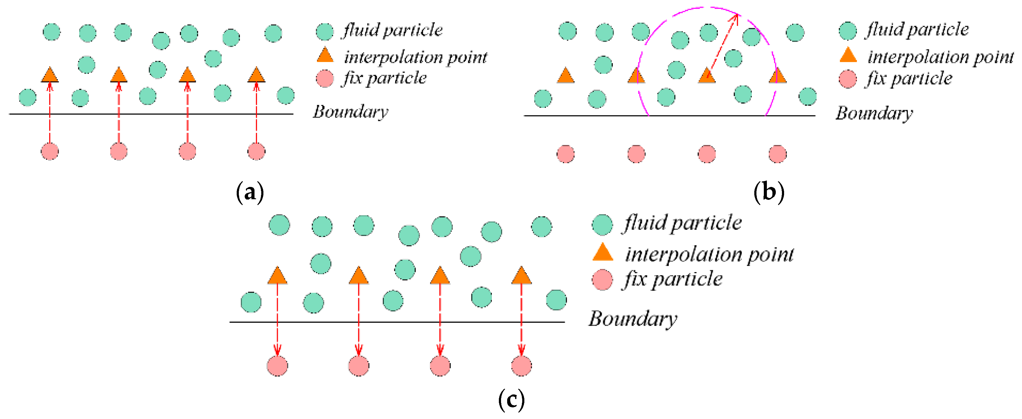
Fixed ghost particles, mirror particles of fixed ghost particles (or interpolation points), interpolation of mirror particles, and laws of mirror are four elements of the fixed ghost boundary method which can be achieved through the following steps (see Figure 1):

(1)

Arrange the fixed ghost particles on the normal unit vector (out of the fluid domain) and distribute mirror particles (i.e., interpolation points) on the opposite direction according to the shape of the surface,

(2)

The physical properties of mirror particles are evaluated through performing interpolation among the fluid particles,

(3)

The physical properties of fixed ghost particles are duplicated from the mirror particles according to the laws of mirror.

It is possible to enforce the Dirichlet condition by the fixed ghost particle method. For the free-slip condition, the tangential velocity component did not change during the mirroring procedure and the normal velocity component was reversed in order to enforce the boundary condition $\mathit{u}·\mathit{n}=0$. For the no-slip condition, both the tangential velocity component and the normal velocity component were reversed. The assignment of pressure field of the fixed ghost particle method obeyed the Neumann condition, i.e., $\partial \mathit{p}/\partial \mathit{n}=\rho \mathit{f}·\mathit{n}$.

A more detailed description of the fixed ghost particle method for special shape and handling method were provided by Marrone (2011, [15]), Chen (2017, [5]), and Kolerski (2013, [33]).

3. Boundary Interpolation Method

3.1. Moving Least Squares (MLS) Method

The moving least squares (MLS) method is a widely used interpolation scheme (Colagrossi, 2003, [16]), and the pressure of the interpolation point is evaluated as follows:

$${\mathrm{P}}_G={\displaystyle \sum _{j\in fluid}{p}_j{W}^{MLS}\left({\mathit{r}}_j\right)V_j+d\rho \mathit{g}·\mathit{n}}$$

(8)

where d is the distance between the interpolation point and its corresponding fixed ghost particle.

The moving least squares kernel W^MLS is given by:

$$\{\begin{array}{ll}{W}^{MLS}(r_j)={\mathit{M}}_i{}^{-1}{\mathit{e}}_1·{\mathit{b}}_{ij}W(r_j)& \\ b_{ij}{}^T=[1,(x_j-x_i),(y_j-y_i),(z_j-z_i)];& {\mathit{e}}_1{}^T=[1,0,0,0]\\ {\mathit{M}}_i={\displaystyle \sum _j{\mathit{b}}_{ij}\otimes {\mathit{b}}_{ij}W(r_j)d{V}_j}& \end{array}$$

(9)

The solution process of W^MLS is very complex which includes a variety of operations like the tensor product, sum of matrices, and inverse of the matrix. The MLS method has the following shortcomings. First, if the sample size is less than the characteristic number, the fitting equation is under-determined and the equations with an inverse matrix do not exist. For the linear basis function, the characteristic number is three, and for the quadratic basis function, the characteristic number is six, that is, when the number of particles in the interpolating domain is less than the characteristic number, the solution will fail. Secondarily, the numerical results are unstable because of the singular or morbid state of the matrix in the process of matrix inversion. Thirdly, this method uses a large amount of calculations and has a low computational efficiency, and the calculated amount shows a quadratic relationship with the number of adjacent particles.

3.2. Simplified Finite Difference Interpolation (SFDI) Method

The SFDI method is another useful method for an interpolation scheme which is cheaper to compute than the MLS scheme, mainly because the matrix inverse is not involved (Ma, 2008, [19]). The relevant key formulas are summarized as follows:

$$f\left(\mathit{r}\right)={\displaystyle {\sum }_{J=1}^N{\mathsf{\Phi }}_j\left(\mathit{r};{\mathit{r}}_i\right)f\left({\mathit{r}}_{\mathit{j}}\right)}$$

(10)

where ${\mathsf{\Phi }}_J\left(\mathit{r};{\mathit{r}}_{\mathit{i}}\right)$ is the shape function in the SFDI interpolation and is defined by

$${\mathsf{\Phi }}_j\left(\mathit{r};{\mathit{r}}_i\right)=\frac{w\left(\left|{\mathit{r}}_j-\mathit{r}\right|\right)}{{\displaystyle {\sum }_j^{n}w\left(\left|{\mathit{r}}_j-\mathit{r}\right|\right)}}-\left(1-{\delta }_{ij}\right)B_{0,j}\left({\mathit{r}}_i\right)+{\delta }_{ij}{\displaystyle {\sum }_{j\ne i}^n{B}_{0,j}\left({\mathit{r}}_i\right)}$$

(11)

where the position vector of a particle represented by ${\mathit{r}}_i$ that is taken as the nearest one to the point $\mathit{r}$, ${\delta }_{ij}=\{\begin{array}{c}1i=j\\ 0i\ne j\end{array}$, $B_{0,j}\left({\mathit{r}}_i\right)=\frac{w\left(\left|{\mathit{r}}_j-{\mathit{r}}_i\right|\right)}{{\left|{\mathit{r}}_j-{\mathit{r}}_i\right|}^2}{\displaystyle {\sum }_{k=1}^2\frac{{\mathit{R}}_{0,x_k}}{n_{i,x_k}}}\left({\mathit{r}}_{j,x_k}-{\mathit{r}}_{i,x_k}\right)$ and

$${\mathit{R}}_{0,x_k}=\frac{{\displaystyle {\sum }_j^n\left({\mathit{r}}_{j,x_k}-{\mathit{r}}_{x_k}\right)w\left(\left|{\mathit{r}}_j-\mathit{r}\right|\right)}}{{\displaystyle {\sum }_j^{n}w\left(\left|{\mathit{r}}_j-\mathit{r}\right|\right)}}$$

(12)

Similar to the MLS method, for the consistency of the formula form, we defined: $W^{\mathrm{SFDI}}\left(r_j\right)={\mathsf{\Phi }}_j\left({\mathit{r}}_0;{\mathit{r}}_i\right)$, the pressure of the interpolation point is evaluated as follows

$${\mathrm{P}}_G={\displaystyle \sum _{j\in fluid}{p}_j{W}^{\mathrm{SFDI}}\left(r_j\right)+2d\rho \mathit{g}·\mathit{n}}$$

(13)

Different from the way in which the MLS method is used to inverse the matrix, the SFDI method effectively improves the stability of the interpolation operation by adopting the Taylor series expansion (Zheng, 2017, [21]), and reduces the required calculation time. However, since solving equations with W^SFDI contains many summation parameters, the computational complexity of this method is a quadratic relationship with the number of neighboring particles.

3.3. Normalized Interpolation Method

The normalized interpolation method is a well-known method in the SPH family. For boundary particles and/or irregularly distributed particles, it will be unable to satisfy the normalization and symmetry conditions (Wen, 2016, [24]). To overcome these problems, it has been used here with the corrective kernel approximation of a function given by

$$f_i=\frac{{\displaystyle {\sum }_{j=1}^n{f}_j}{W}_{ij}{V}_j}{{\displaystyle {\sum }_{j=1}^n{W}_{ij}{V}_j}}={\displaystyle {\sum }_{j=1}^n{f}_j}{\tilde{W}}_{ij}{V}_j$$

(14)

where the modified kernel function ${\tilde{W}}_{ij}$ can be written as:

$${\tilde{W}}_{ij}=\frac{W_{ij}}{{\displaystyle {\sum }_{j=1}^n{W}_{ij}{V}_j}}$$

(15)

The pressure of the interpolation point is evaluated as follows:

$${\mathrm{P}}_G={\displaystyle \sum _{j\in fluid}{p}_j\tilde{W}\left(r_j\right)V_j+2d\rho \mathit{g}·\mathit{n}}$$

(16)

Different from the MLS method, there is no need for a normalized interpolation method to perform the inverse operation when using the kernel function which makes the method have better stability. In addition, the solution for this method is relatively simple compared with the SFDI method, and obtains better computational efficiency. The calculation amount of the ${\tilde{W}}_{ij}$ method changes linearly with the number of neighboring particles. However, the low accuracy of the numerical results has become a significant disadvantage to this approach.

3.4. Improved Shepard Interpolation Method

The improved Shepard interpolation method will be presented in this section. According to the Shepard method (Shepard, 1968, [34]), physical properties at any arbitrary point are obtained through the function:

$$f\left(x\right)=\{\begin{array}{ll}\frac{{\displaystyle {\sum }_{j=1}^n{r}_i{}^{-\mu }}f\left(x_j\right)}{{\displaystyle {\sum }_{j=1}^n{r}_i{}^{-\mu }}}\hfill & r_i\ne 0\hfill \\ f\left(x_i\right)\hfill & r_i=0\hfill \end{array}$$

(17)

where $r_i=\sqrt{{(x-x_i)}^2+{(y-y_i)}^2}$ within 2-D space, μ > 0 is the power parameter.

Assuming that $\phi (r_i)=r_i{}^{-1}$, then the weighting functions can be defined as:

$$W^{shepard}\left(x_i\right)=\frac{r_i{}^{-\mu }}{{\displaystyle {\sum }_{i=1}^n{r}_i{}^{-\mu }}}=\frac{\phi {(r_i)}^{\mu }}{{\displaystyle {\sum }_{i=1}^n\phi {(r_i)}^{\mu }}}$$

(18)

The weighting functions W^shepard(x_i) are at least C⁰ continuous (Lodha, 1997, [35]) and the power parameter is set to two because this makes the Shepard interpolation be optimal in a certain sense among all stable rational interpolation schemes (Farwig, 1986, [36]). In order to ensure the continuity of the weighting functions and their derivatives, and the continuity of the physical properties of the mirror particle, μ = 4 was used in this paper.

Similar to the properties of kernel functions in the SPH method, the Shepard weighting function should be compactly supported in order to enhance the computational efficiency and reduce the impact of remote particles on the interpolation point. Franke (1980, [37]) modified the weighting function so that it was compactly supported and Kang (2011, [27]) proposed a guideline about the choice of the influence domain. In order to satisfy Newton’s third law, the influence domain of the weight function should correspond to the support domain of the kernel function of the SPH method.

An improved Shepard method which has a higher smoothness and a better attenuation is used in this paper:

$$\phi (r_i)=\beta (r_i)\frac{1}{r_i}$$

(19)

$$\beta \left(x_i\right)=\{\begin{array}{ll}{e}^{-\frac{r_i^2}{1-{\left(\frac{r_i}{R}\right)}^{\lambda }}}\hfill & 0\le r_i\le R\hfill \\ 0\hfill & r_i>R\hfill \end{array}$$

(20)

where R is the influence domain which is equal to δ in Equation (7), and λ is an adjustment index which can change the attenuation of W^shepard.

Therefore, the pressure of a generic ghost particle is evaluated as follows:

$${\mathrm{P}}_G={\displaystyle \sum _{j\in fluid}{p}_j{W}^{shepard}\left(r_j\right)V_j+2d\rho \mathit{g}·\mathit{n}}$$

(21)

Since matrix inversion is not required in this method, the improved Shepard method obtains a better numerical stability and robustness than the MLS method. By using a direct summation form, the improved Shepard method also has higher computational efficiency than the MLS method and the calculated amount of the central particle also has a linear relationship with the number of neighboring particles.

In this study, we found that the improved Shepard method had a better computation efficiency than the MLS method or the simplified finite different interpolation method, as shown in

Table 1. Comparisons of calculated amount.

Interpolation Method	Calculated Amount (Relationship with Neighboring Particles)
Moving Least Squares method	Quadratic
Simplified Finite Difference Interpolation method	Quadratic
Normalized interpolation method	Linear
Improved Shepard method	Linear

. Moreover, compared to the normalized interpolation method, the improved Shepard method had higher precision in the case of similar time consumption (Xu, 2010, [26]). In addition, instead of interpolation by the nearest particle assignment or by changing interpolation methods when the number of the interpolation particle was less than the characteristic number, the improved Shepard algorithm kept a better stability and robustness of the interpolation results by means of distance weighted average evaluation.

4. Numerical Results

4.1. Hydrostatic Tank Test

Similar to the test of Chen et al. (2015, [38]), a simple two-dimensional rectangular hydrostatic test was used to show the accuracy and efficiency gap between and MLS method, FSDI method, normalized method, and the improved Shepard method. This test case ran on a CPU (Central Processing Unit) with an Intel(R) Xeon(R) E3-1230 [email protected] GHz processor, 16 GB of memory, and a 64-bit Windows OS.

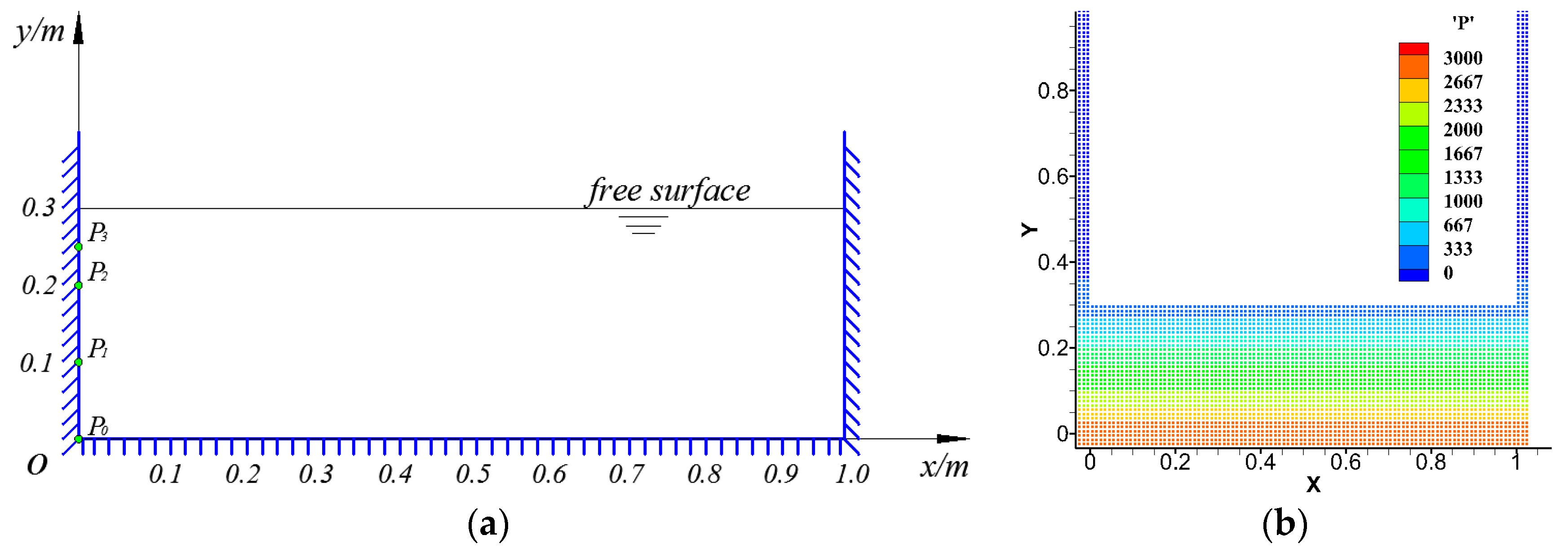
As shown in Figure 2, the length of the model was 1 m and the depth was 0.3 m. This test was also computed by the standard WCSPH with artificial viscosity (α = 0.02). The initial distance between particles was Δx = Δy = 0.01 m, with h = 1.30 Δx, and a time step equal to 10⁻⁴ s. The simulation ended at the physical time 35 s. The model is given by Figure 2, and four pressure detection points P₀ (0, 0), P₁ (0, 0.1), P₂ (0, 0.2), and P₃ (0, 0.25) are set on the left vertical wall.

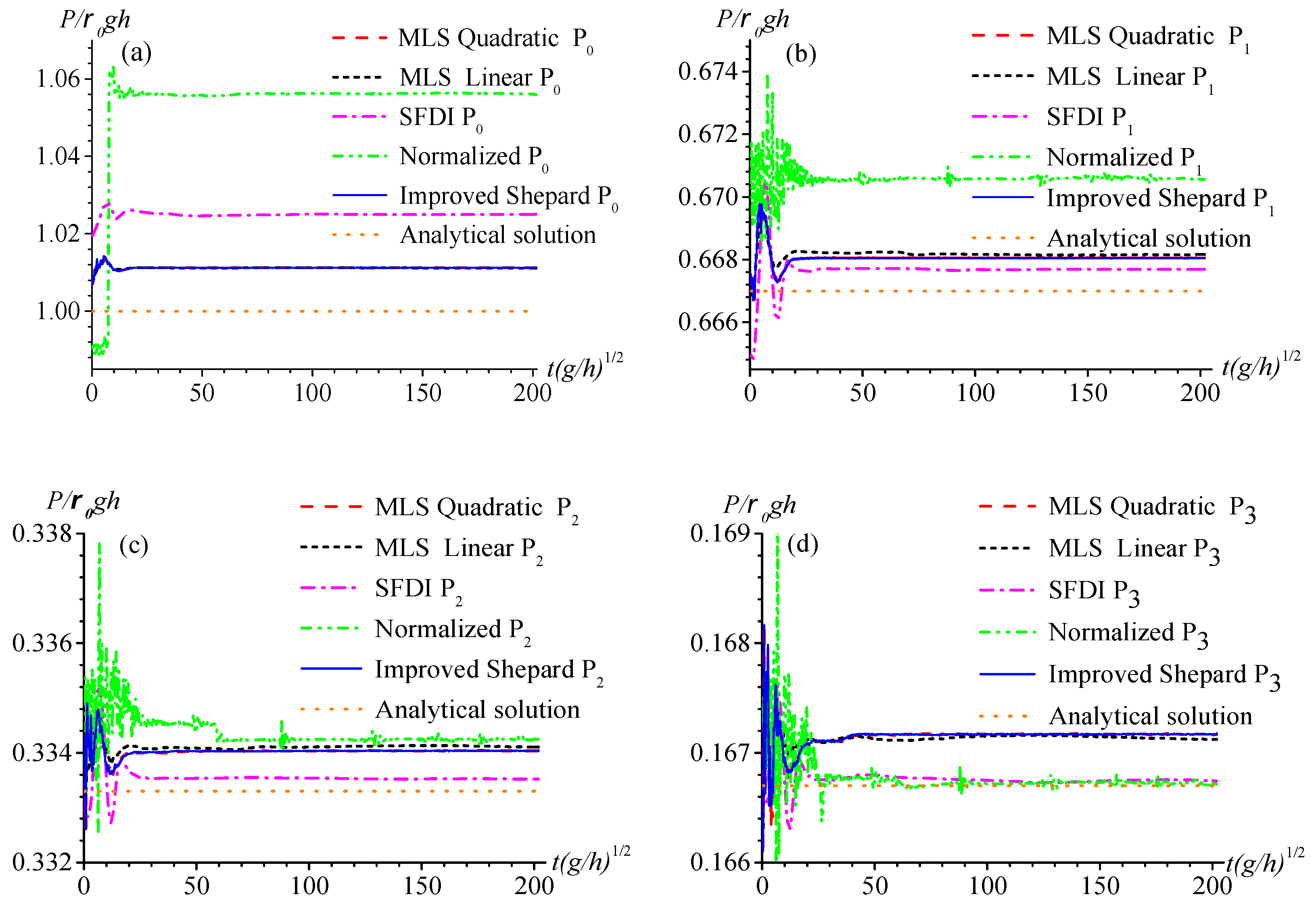
Figure 3 shows the history of static water pressure recorded at P₀, P₁, P₂, and P₃ using the different interpolation methods and the analytical solution. Influenced by the accuracy of interpolation methods, the stability of the pressure numerical results obtained by several interpolation methods were different. The normalized method had a lower interpolation precision, and the initial moment pressure showed obvious oscillation, while the pressure field always had slight fluctuations. In the SFDI method, the pressure results also showed significant oscillations at the initial moment. In comparison, the MLS method and the improved Shepard method had relatively stable pressure results, and the numerical values of the improved method were basically consistent with the numerical results of the MLS quadratic method, indicating that the improved Shepard method has good numerical accuracy.

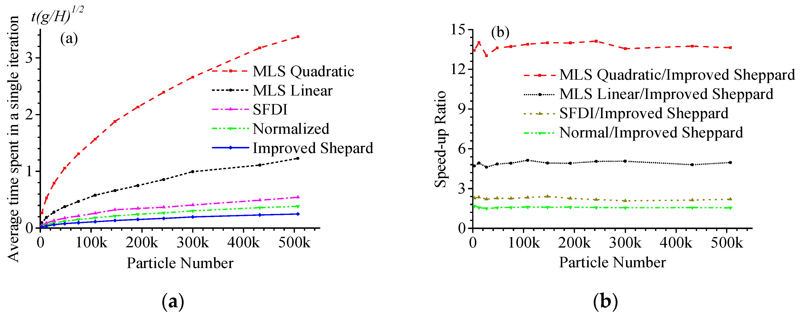
Figure 4a shows the average single-step calculation time for each method with different numbers of particles. As the number of particles increased, the calculation time of the MLS method increased rapidly, especially for the quadratic basis method. The time-consuming and inefficient algorithm was not conducive to the application of the SPH method. Compared with the MLS method, the SFDI method, normalized method, and the improved Shepard method exhibited obvious characteristics of low-time consumption and high efficiency. Further, it can be seen from the speed-up ratio (the ratio of the calculation time of each method to the improved Shepard method under the same conditions) that the calculation speed of the improved Shepard method was more than twice that of the SFDI method and 1.5 times that of the normalized method.

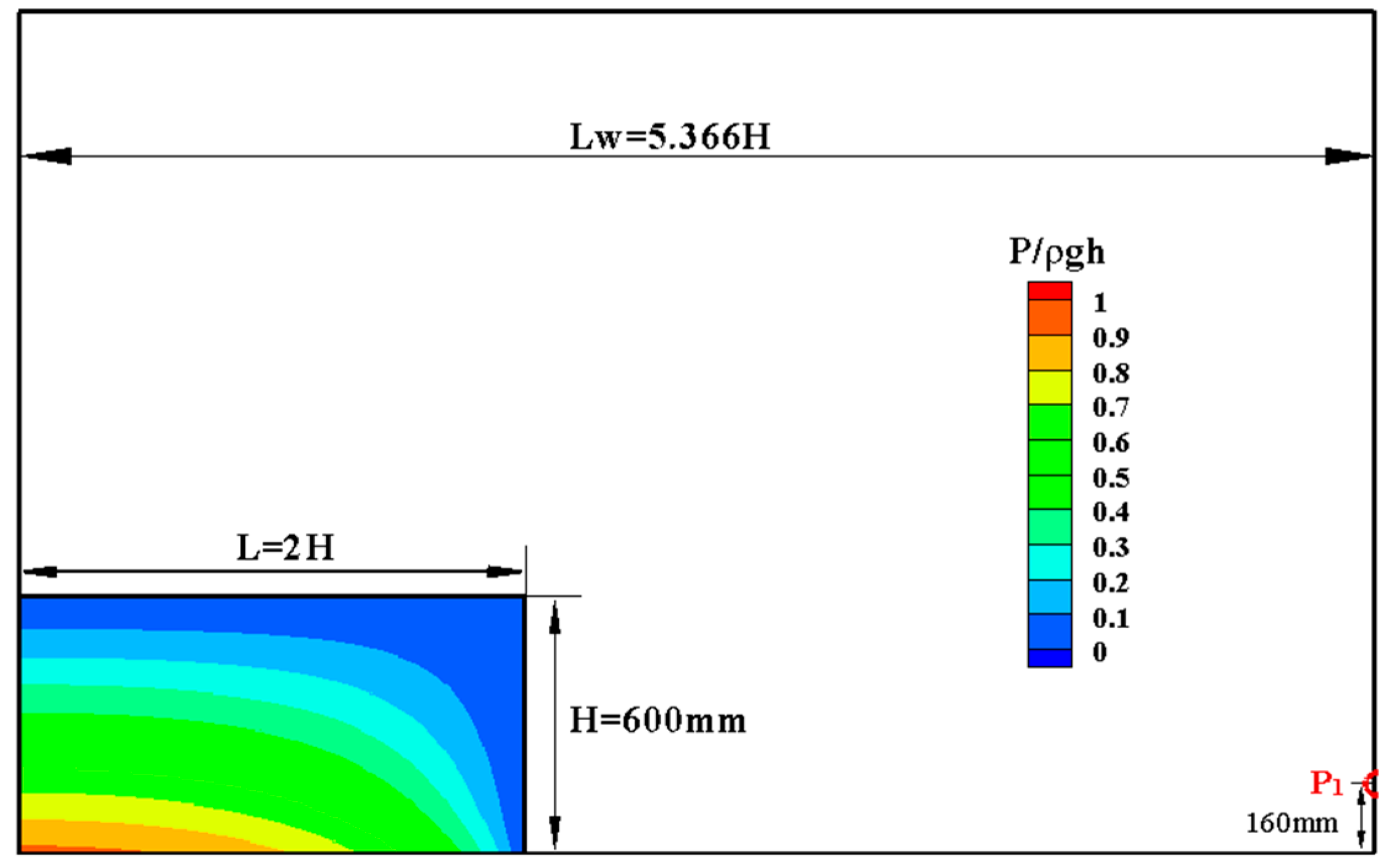
4.2. Dam-Breaking Problem

Dam break flow is a well-known practical and analytical free-surface flow problem used to validate the effectiveness of the improved Shepard method. The schematic setup of the problem is depicted in Figure 5, where a rectangular column of water was confined. The width of the water column was L and the height of this water column was H. At the beginning of the computation, the dam instantaneously collapsed. The pressure sensor P₁ was chosen for the right wall according to the experimental results of Buchner (2002, [39]).

In this section, H = 0.6 m, L/H = 2.0, and L_w = 5.366H were used. The initial distance between particles was Δx = Δy = 0.004 m and the total particle number was 45,000. The time step equaled 10⁻⁴ s and the speed of sound C₀ was equal to $20\sqrt{gH}$.

Considering the weakly compressible fluids hypothesis, an improved initial density field assignment method was adopted by combing it with the Laplace equation and the equation of state in this paper. When the baffle was opened, the pressure should have obeyed the Laplace equation, and the top and right side of the water column did become free surface, namely, the pressure was zero along these sides, and the normal pressure gradient on the left side of the border and bottom of the water column was 0 and −ρg, respectively. In addition, the equation of state should also be satisfied. Therefore, the initial control equation is shown as follows:

$$\{\begin{array}{ll}{\nabla }^{2}P=0\hfill & \left(0<x<\mathrm{L},0<y<H\right)\hfill \\ \frac{\partial P}{\partial y}=-\rho g\hfill & \left(0<x<L,y=0\right)\hfill \\ \frac{\partial P}{\partial x}=0\hfill & \left(x=0,0<y<H\right)\hfill \\ P=0\hfill & \left(x=L \mathrm{or} y=H\right)\hfill \\ P=c_0{}^2(\rho -{\rho }_0)\hfill & \mathrm{on}\mathrm{the}\mathrm{field}\hfill \end{array}$$

(22)

The expression of initial density can be obtained as follows:

$$\rho ={\rho }_0+{\displaystyle \sum _{\mathrm{n}=0}^{\infty }{\alpha }_n\cos ({\lambda }_{n}x)\sinh }{\lambda }_n(H-y)$$

(23)

where

$${\alpha }_n=\frac{{\rho }_{0}g\sin ({\lambda }_{n}x)}{{\lambda }_n(c_0{}^2{\lambda }_n\cosh ({\lambda }_{n}H)-g\sinh ({\lambda }_{n}H))(0.5L+\sin (2{\lambda }_{n}L)/4{\lambda }_n)}$$

(24)

$${\lambda }_n=(\mathrm{n}+\frac{1}{2})\frac{\pi }{L},(n=0,1,2\dots )$$

(25)

The expression of initial pressure can be obtained by combining Equation (23) and the equation of state and shown in Figure 5.

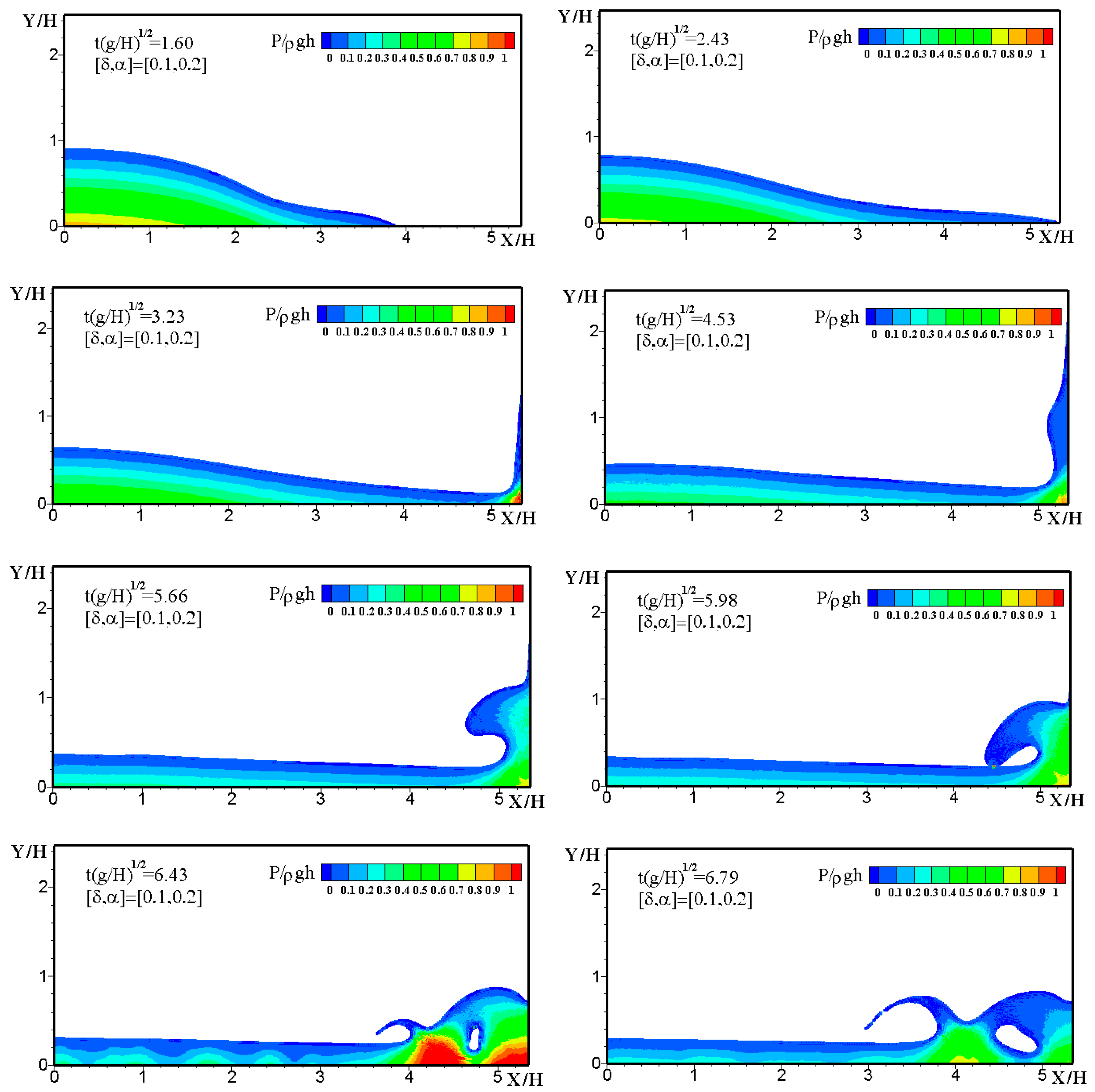
Figure 6 gives several snapshots at different times which show the evolution of the free surface. As the calculation advances, the water column collapses and the free surface evolves freely under the action of gravity. The front end of the flow touches the right vertical wall (which occurs at about $t\sqrt{g/H}=2.43$) and begins to climb. The plunging wave closure forms a closed hole (which occurs at about $t\sqrt{g/H}=5.98$). It is clear that, by using the improved initial density field assignment method, the fluid pressure field remained stable during the collapse process.

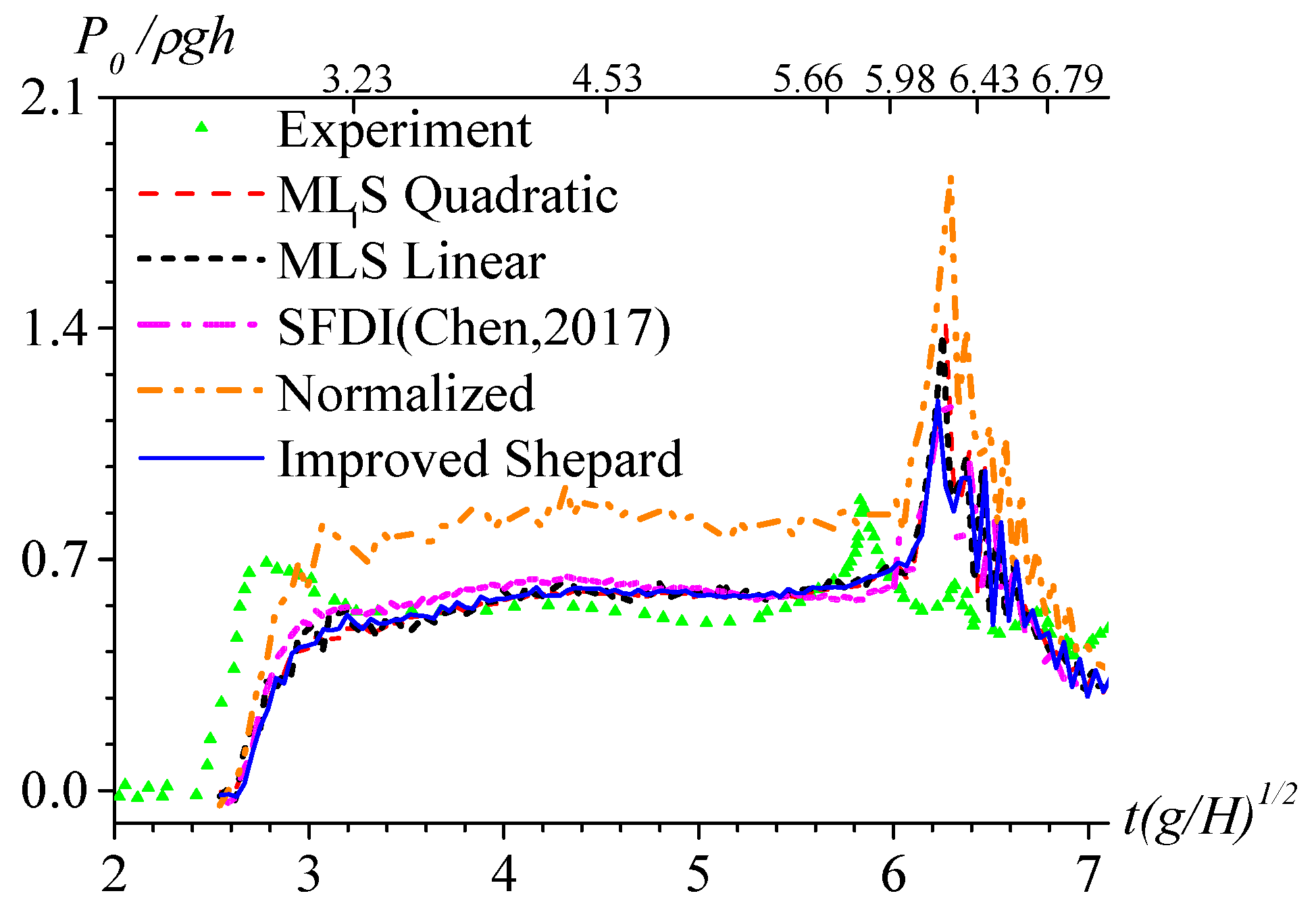
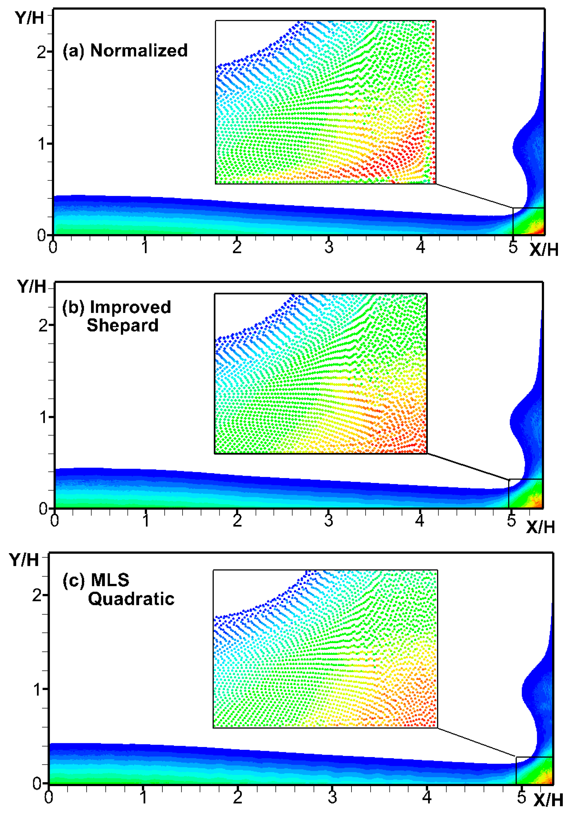
Figure 7 shows the time–history curves of dynamic pressure results on P₁ from experimental data and different numerical methods. All of the interpolation methods recorded the pressure change during the free-surface climb and the plunging wave closure. The MLS method, the SFDI method (Chen, 2017, [5]), and the improved Shepard method have similar calculation results, while the normal method provided significantly larger numerical values than other methods. In fact, due to the low precision of the normal method, the pressure value of the particle point had deviations at the wall surface, and the flow field pressure resulted in unstable oscillation. As shown in Figure 8, the pressure field of the improved Shepard method and the MLS method showed better continuity and stability than the normalized method. In addition, according to Ren (2016, [40]) and Philip (1999, [41]), that all the numerical results take longer to reach the right side of the straight than the experimental results may be due to that the door is gradually opened during the experiment, while the numerical simulation is instantaneous.

Figure 9 shows the comparison of the average single time step for different interpolation methods during the dam-break process. In this case, the free-surface flow led to an increase in the number of fixed interpolated particles, and the single-step calculation time increased. Unlike the sharp increase in the computational time of the MLS method, the improved Shepard method exhibited the characteristic of approximately linear slow growth. From the comparison of computational efficiency, the improved Shepard method was 1.4 times faster than the normalized method, 1.9 times faster than the SFDI method, 4.2 times faster than the MLS method (linear based), and 11.6 times faster than the MLS method (quadratic based) method at least.

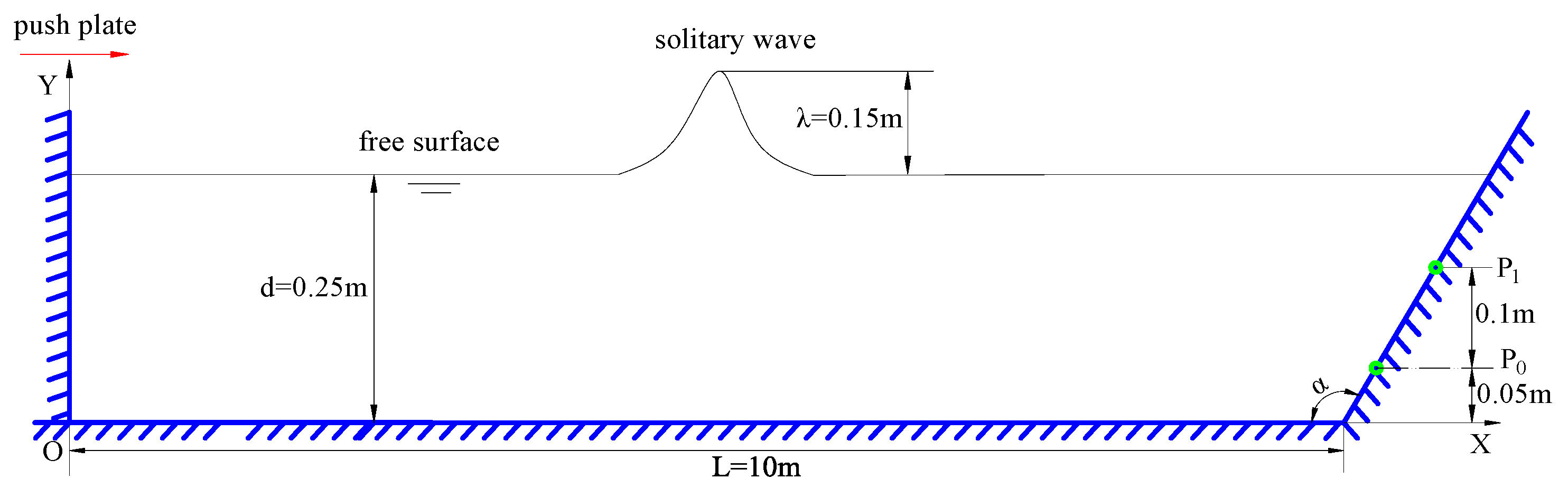
4.3. Solitary Wave Impact on Fixed Seawalls

In consideration of the particle motion characteristics of the SPH method and the truncation of the kernel function on the boundary, the long-distance wave propagation easily leads to the large numerical dissipation of the flow field particles, resulting in large numerical error accumulation. In addition, the stability of the boundary treatment method also plays a key role in the accuracy of the numerical results. Solitary wave is a kind of extreme wave phenomenon in coastal and ocean engineering problems, which is used to represent certain characteristics of the tsunami wave (Lin, 2015, [42]). In this section, the solitary wave propagation over a constant water depth and impact on a solid wall is considered to verify the effectiveness and stability of the improved Shepard method.

The wave simulation physical model is shown in Figure 10, a model with an inclination angle α (α = 120°) on the right wall is used to verify the ability of the improved Shepard method to deal with complex boundaries. The common basic information of the model was as follows: the length of the tank model was 10 m, the depth of the water was 0.25 m, two measurement points were located on the right wall at a distance of y = 0.05 m (P₀) and y = 0.15 m (P₁) to monitor the pressure time history for comparison with the numerical results of Chen (2017, [5]) and the experimental results of Zheng (2015, [43]). Besides, in order to compare the effect of different interpolation methods on the stability of the pressure results, the MLS method (both linear-based and quadratic-based) and SFDI method were also used in this part.

The solitary wave height was λ = 0.15 m and the wave non-linearity was ε = λ/d = 0.6. The particle spacing was dx = 0.01 m, the particle size was 0.0001 m and the time step equaled 0.0001 s. The fluid particle number was 25,180.

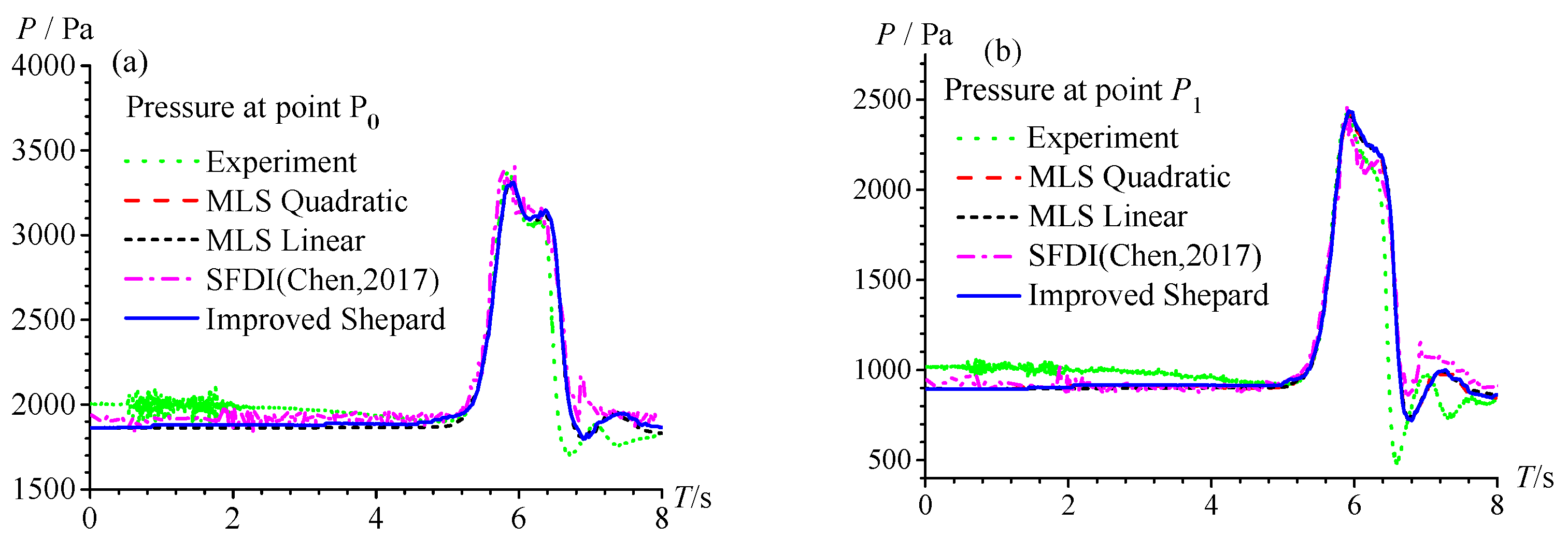
Figure 11 gives the comparison of pressure time histories at P₀ and P₁. From the results in both figures, it shows that the improved Shepard method can achieve good results compared with the experimental data in the process of wave peak transmission.

The results show that compared with the unstable pressure results of the SFDI method by Chen (2017, [5]), the difference between the improved Shepard method and the MLS method was small and coincided well in this paper. Although the interpolation accuracy of the MLS algorithm was higher than that of the Shepard method in mathematics, the high-precision algorithm easily generated a singular matrix when the number of particles was small or the particles were irregularly distributed, which affected the stability and accuracy of the calculation results. In comparison, the calculation results reflected the good numerical stability and robustness of the improved Shepard method.

As shown in Figure 12, the improved Shepard method was still the most efficient method among several methods in terms of computational efficiency. The computational efficiency of improved Shepard method was nearly twice faster than that of the SFDI, 3.7 times faster than that of MLS (linear based) method and 9.6 times faster than that of MLS method (quadratic based). Therefore, the improved Shepard method obtained extremely high computational efficiency while ensuring the accuracy of the calculation results.

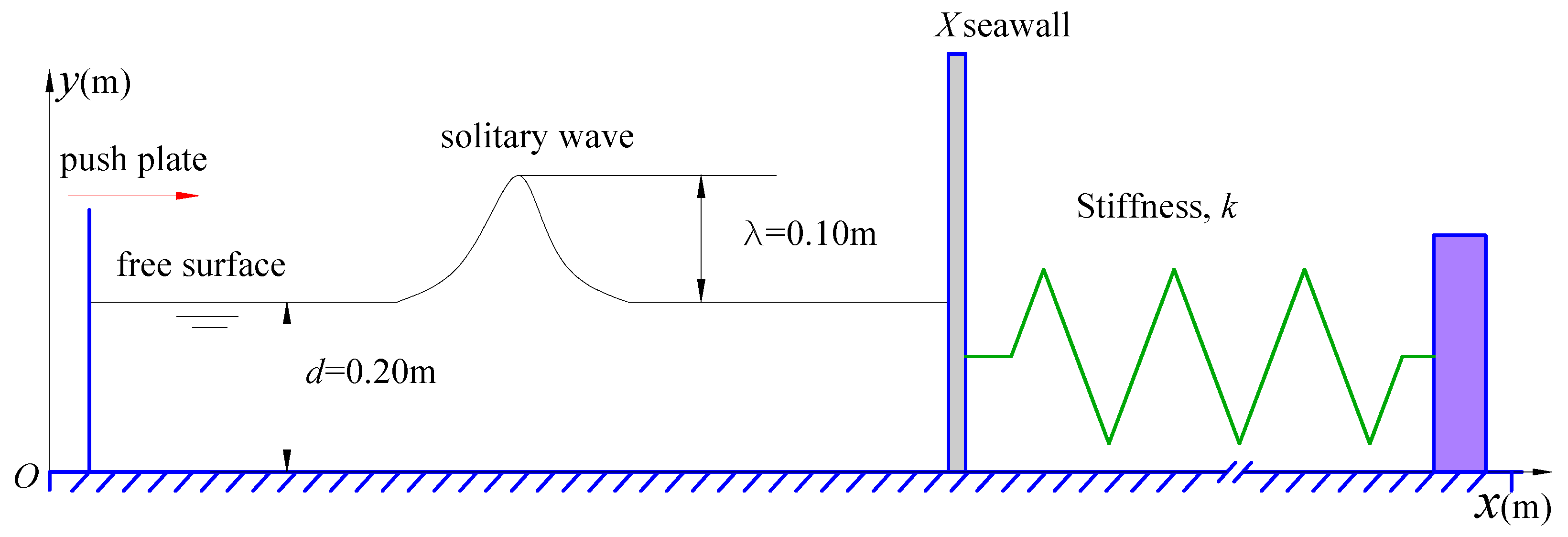
4.4. Solitary Wave Impact on Movable Seawalls

We tested a wave–structure interaction problem associated with a passively moving seawall which was derived from the conceptual design of energy-absorbing tsunami shelters presented in Pimanmas et al. (2010, [44]) and simulated by Liang et al. (2017, [45]) with an incompressible SPH (ISPH) method. The configuration is given in Figure 13. It is assumed that the energy-absorbing connectors behave like an ideal spring and the passively moving seawall is idealized into a simple spring-mass system which consists of a spring attached to a vertical wall. Seawall mass and spring stiffness were the only two parameters used to describe the properties of the movable structure in this simplified model.

The seawall was initially located at $x_{seawall}^0$ = 2.50 m, with a water depth of 0.20 m under hydrostatic conditions, and the spring system was in its relaxed form. When the wave generated by the wave maker begins to propagate to the right side, the impact force on the seawall will change compared with the static water conditions. When the change exceeds a specified threshold value, the seawall will become mobile.

The spring-mass system is used to sustain a certain amount of impact force before it can be compressed according to Liang et al. (2017, [45]). The onset of motion for the system is determined by a threshold force ratio, defined as F_threshold = 1.10 × F_static. The acceleration, velocity, and position of the seawall were calculated as follows:

$$a_{seawall}^n=\{\begin{array}{ll}\frac{\left(F_{impact}^n-F_{threshold}\right)-k·\left(x_{seawall}^n-x_{seawall}^0\right)}{m_{seawall}},\hfill & F_{impact}^n>F_{threshold}\hfill \\ -\frac{k·\left(x_{seawall}^n-x_{seawall}^0\right)}{m_{seawall}},\hfill & F_{impact}^n\le F_{threshold}\hfill \end{array}$$

(26)

$$v_{seawall}^{n+1}=v_{seawall}^n+a_{seawall}^n\mathsf{\Delta }t$$

(27)

$$x_{seawall}^{n+1}=\{\begin{array}{ll}{x}_{seawall}^n+v_{seawall}^{n+1}\mathsf{\Delta }t,\hfill & x_{seawall}^{n+1}>x_{seawall}^0\hfill \\ x_{seawall}^0,\hfill & x_{seawall}^{n+1}\le x_{seawall}^0\hfill \end{array}$$

(28)

where k is the spring stiffness coefficient and m_seawall the mass of seawall. Superscripts n and (n + 1) denote the current and future time steps, respectively.

The following formulation was adopted to evaluate the impact force on vertical walls by Liang et al. (2017, [45]):

$$F_{impact}^n=m_i{\displaystyle \sum _j\frac{m_j}{{\rho }_j}}\left[-\frac{p_j}{{\rho }_j}+\frac{p_i}{{\rho }_i}\right]\times {\nabla }_i{W}_{ij}$$

(29)

The impact force computed by Equation (29) was non-dimensionalized as follows:

$$F*=F_{impact}/F_{static}$$

(30)

where F* is the non-dimensional impact force and F_static denotes the hydrostatic force on the wall.

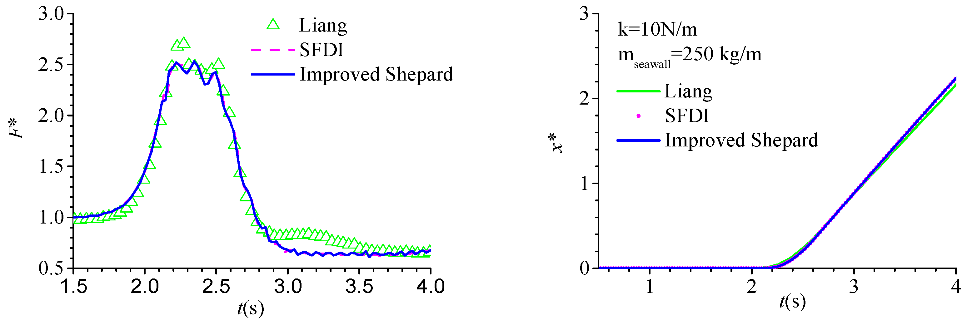
In this paper, the wave condition and seawall properties followed the simulation of Liang et al. (2017, [45]), where seawall mass m_seawall = 250 kg/m and spring stiffness coefficient k = 10 N/m. The initial distance between particles was Δx = Δy = 0.008 m and the total particle number was 8025. The time step equaled 5.0 × 10⁻⁴ s and speed of sound C₀ was equal to $10\sqrt{gH}$.

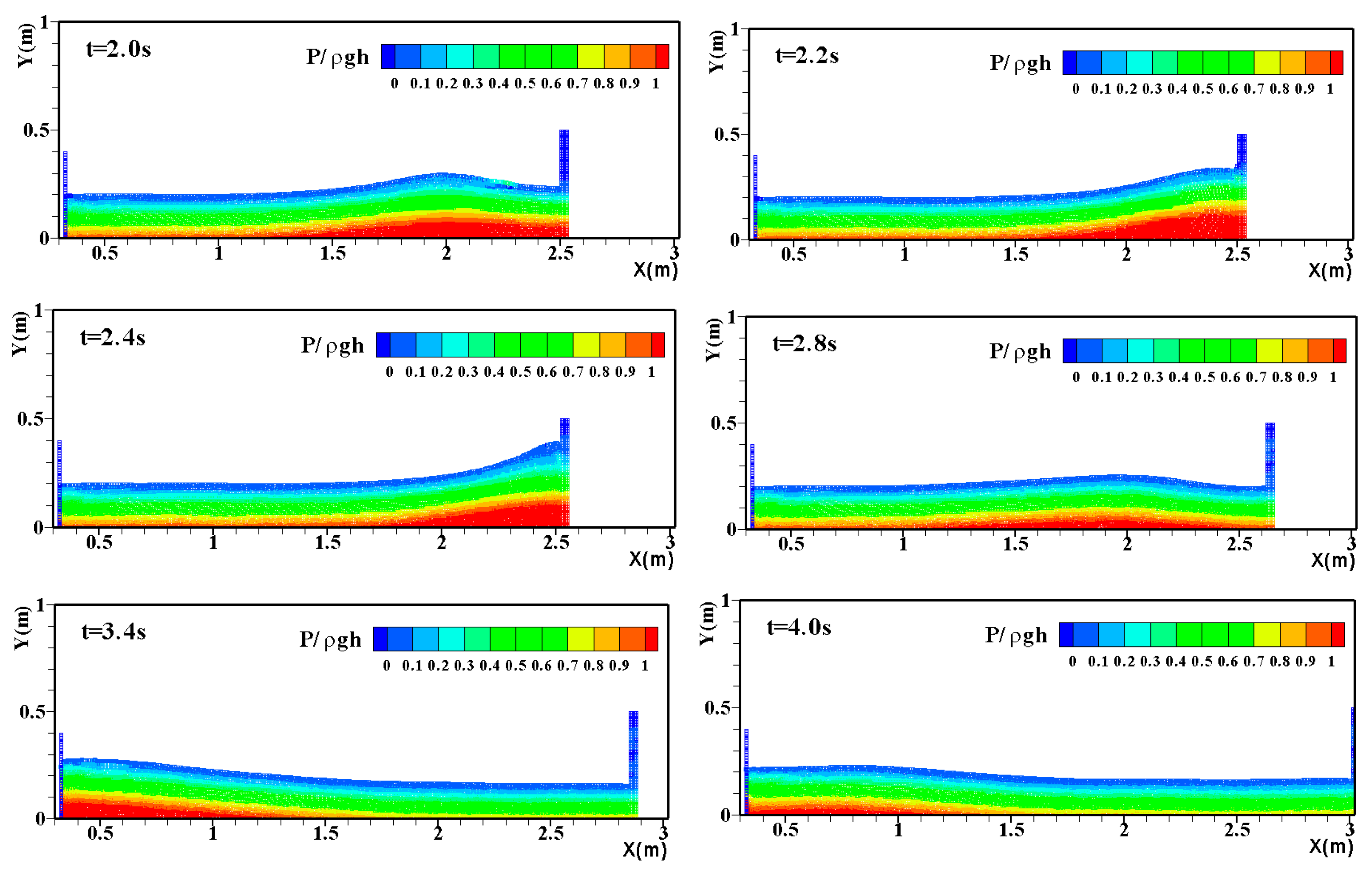
Figure 14 presents some snapshots of the surface profile results with pressure contours using WCSPH. The seawall became mobile between t = 2.00 s and t = 2.20 s. Then, the wave continued to rise, and the pressure of the seabed increased, reaching its peak at about t = 2.4 s. Comparing the surface profiles t = 2.0 s of t = 2.8 s, it can be seen that the reflection wave surface decreased obviously due to the spring-mass system absorbing part of the impact. After that, the reflected waves propagated to the left, and the seawall continued to move to the right, and the location of the seawall was about 2.96 m when t = 4.00 s.

Figure 15 compares the wave force, seawall displacement, and wave run-up at the seawall for the seawall at rest and while in motion. For the purpose of comparison, the experimental data from Liang et al. (2017, [45]) were also plotted. The seawall displacement was non-dimensionalized as: $x*=X/h$, where X denotes the seawall displacement.

From the comparison of forces, it can be seen that the numerical results of the improved Shepard method and the SFDI method were in good agreement in this case and the spring-mass system effectively reduced the impact force acting on the seawall by the solitary wave. The results for force match well the result of Liang et al. (2017, [45]) before 2.8 s. After that, due to the influence of particle compression, the velocity difference of the push plate was faster than that of Liang et al. (2017, [45]), as shown on seawall displacement, and the pressure obviously decreased. There was a small gap between this value and the results of Liang et al. (2017, [45]), which may have been influenced by the difference between the weakly compressible SPH method and the incompressible SPH method. In addition, considering the calculation efficiency, in this case, the average calculation time of the improved Shepard method was at least 1.8 times faster than that of the SFDI method, which reflects the high efficiency of the improved Shepard method.

5. Conclusions and Discussions

An efficient and stable boundary processing method was introduced by embedding the improved Shepard method into the interpolation of physical quantities of boundary-fixed particles for the SPH method in this paper. A rectangular hydrostatic tank was used to compare the calculation accuracy and efficiency between the MLS method, normalized method, SFDI method, and improved Shepard method. Furthermore, for comparing these four kinds of interpolation methods, a benchmark model of dam-breaking with a new initial flow field arrangement formula was considered. Finally, the solitary wave impact on a fixed wall with different inclination angles and a moveable wall with a spring-mass system was also adopted with different interpolation methods.

The results illustrate that applying the improved Shepard method to the SPH method can achieve good calculation precision results which are closer to the MLS method when compared with the normalized method and the SFDI method. Secondly, by using a simple summation operation process, the computational efficiency of the improved Shepard method was much higher than the MLS method, SFDI method, and even more than half faster than the normalized method. Thirdly, since there was no need for matrix inversion, the improved Shepard method had better stability and robustness than the MLS method.

References

- Lucy, L.B. A numerical approach to testing of fission hypothesis. Astron. J. 1977, 82, 1013–1024. [Google Scholar] [CrossRef]
- Gingold, R.A.; Monaghan, J.J. Smoothed particle hydrodynamics: Theory and application to non-spherical stars. Mon. Not. R. Astron. Soc. 1977, 181, 45–58. [Google Scholar] [CrossRef]
- Monaghan, J.J. Simulating free surface flows with SPH. J. Comput. Phys. 1994, 110, 399–406. [Google Scholar] [CrossRef]
- Monaghan, J.J. Smoothed particle hydrodynamics. Rep. Prog. Phys. 2005, 68, 1703–1758. [Google Scholar] [CrossRef]
- Chen, Y.S.; Zheng, X.; Jin, S.Q.; Duan, W.Y. A corrected solid boundary treatment method for Smoothed Particle Hydrodynamics. China Ocean Eng. 2017, 31, 238–247. [Google Scholar] [CrossRef]
- Padova, D.D.; Mossa, M.; Sibilla, S. SPH numerical investigation of characteristics of hydraulic jumps. Environ. Fluid Mech. 2018, 18, 849–870. [Google Scholar] [CrossRef]
- Padova, D.D.; Brocchini, M.; Buriani, F.; Corvaro, S.; Serio, D.F.; Mossa, M.; Sibilla, S. Experimental and numerical investigation of pre-breaking and breaking vorticity within a plunging breaker. Water 2018, 10, 387. [Google Scholar] [CrossRef]
- Antuono, M.; Colagrossi, A.; Marrone, S. Numerical diffusive terms in weakly-compressible SPH schemes. Comput. Phys. Commun. 2012, 183, 2570–2580. [Google Scholar] [CrossRef]
- Padova, D.D.; Mossa, M.; Sibilla, S. SPH modelling of hydraulic jump oscillations at an abrupt drop. Water 2017, 9, 790. [Google Scholar] [CrossRef]
- Padova, D.D.; Mossa, M.; Sibilla, S. SPH numerical investigation of the characteristics of an oscillating hydraulic jump at an abrupt drop. J. Hydrodyn. 2018, 30, 106–113. [Google Scholar] [CrossRef]
- Zheng, X.; Duan, W.Y.; Ma, Q.W. Comparison of improved meshless interpolation schemes for SPH method and accuracy analysis. J. Mar. Sci. Appl. 2010, 9, 223–230. [Google Scholar] [CrossRef]
- Sun, P.; Ming, F.; Zhang, A. Numerical simulation of interactions between free surface and rigid body using a robust SPH method. Ocean Eng. 2015, 98, 32–49. [Google Scholar] [CrossRef]
- Hashemi, M.R.; Fatehi, R.; Manzari, M.T. A modified SPH method for simulating motion of rigid bodies in Newtonian fluid flows. Int. J. Non-Linear Mech. 2012, 47, 626–638. [Google Scholar] [CrossRef]
- Monaghan, J.J.; Kajtar, J.B. SPH particle boundary forces for arbitrary boundaries. Comput. Phys. Commun. 2009, 180, 1811–1820. [Google Scholar] [CrossRef]
- Marrone, S.; Antuono, M.; Colagrossi, A.; Colicchio, G.; Le Touzé, D.; Graziani, G. δ-SPH model for simulating violent impact flows. Comput. Methods Appl. Mech. 2011, 200, 1526–1542. [Google Scholar] [CrossRef]
- Colagrossi, A.; Landrini, M. Numerical simulation of interfacial flows by smoothed. J. Comput. Phys. 2003, 191, 448–475. [Google Scholar] [CrossRef]
- Bouscasse, B.; Colagrossi, A.; Marrone, S.; Antuono, M. Nonlinear water wave interaction with floating bodies in SPH. J. Fluid Struct. 2013, 42, 112–129. [Google Scholar] [CrossRef]
- Zheng, X. An Investigation of Improved SPH and Its Application for Free Surface Flow. Ph.D. Thesis, Harbin Engineering University, Harbin, China, 2010. [Google Scholar]
- Ma, Q.W. A New Meshless Interpolation Scheme for MLPG_R Method. CMES 2008, 23, 75–89. [Google Scholar]
- Sriram, V.; Ma, Q.W. Improved MLPG_R method for simulating 2D interaction between violent waves and elastic structures. J. Comput. Phys. 2012, 231, 7650–7670. [Google Scholar] [CrossRef]
- Zheng, X.; Ma, Q.W.; Shao, S.D.; Khayyer, A. Modelling of Violent Water Wave Propagation and Impact by Incompressible SPH with First-Order Consistent Kernel Interpolation Scheme. Water 2017, 9, 400. [Google Scholar] [CrossRef]
- Zhang, N.B.; Zheng, X.; Ma, Q.W.; Duan, W.Y.; Khayyer, A.; Lv, X.P.; Shao, S.D. A hybrid stabilization technique for simulating water wave—Structure interaction by incompressible Smoothed Particle Hydrodynamics (ISPH) method. J. Hydro-Environ. Res. 2018, 18, 77–94. [Google Scholar] [CrossRef]
- Chen, J.; Beraun, J.; Carney, T. A corrective smoothed particle method for boundary value problems in heat conduction. Int. J. Numer. Methods Eng. 1999, 46, 231–252. [Google Scholar] [CrossRef]
- Wen, H.J.; Ren, B.; Dong, P.; Wang, Y.X. A SPH numerical wave basin for modeling wave-structure interactions. Appl. Ocean Res. 2016, 59, 366–377. [Google Scholar] [CrossRef] [Green Version]
- Xu, R.; Stansby, P.; Laurence, D. Accuracy and stability in incompressible SPH (ISPH) based on the projection method and a new approach. J. Comput. Phys. 2009, 228, 6703–6725. [Google Scholar] [CrossRef]
- Xu, Z.Y.; Jian, G.Y.; Zhao, L.; Ding, F.X. Improved Shepard Method and Its Application in Gravity Field Data Interpolation. Geomat. Inf. Sci. Wuhan Univ. 2010, 35, 477–480. [Google Scholar]
- Kang, Z.; Wang, Y.Q. Structural topology optimization based on non-local Shepard interpolation of density field. Comput. Methods Appl. Mech. Eng. 2011, 200, 3515–3525. [Google Scholar] [CrossRef]
- Kang, Z.; Wang, Y.Q. A nodal variable method of structural topology optimization based on Shepard interpolant. Int. J. Numer. Methods Eng. 2012, 90, 329–342. [Google Scholar] [CrossRef]
- Monaghan, J.; Kos, A. Solitary waves on a Cretan beach. J. Waterw. Port Coast. Ocean Eng. 1999, 125, 145–154. [Google Scholar] [CrossRef]
- Molteni, D.; Colagrossi, A.; Colicchio, G. On the use of an alternative water state equation in SPH. In Proceedings of the SPHERIC, 2nd International Workshop, Universidad Politécnica de Madrid, Getafe, Spain, 23–25 May 2007. [Google Scholar]
- Antuono, M.; Colagrossi, A.; Marrone, S.; Molteni, D. Free-surface flows solved by means of SPH schemes with numerical diffusive terms. Comput. Phys. Commun. 2010, 181, 532–549. [Google Scholar] [CrossRef]
- Morris, J.P. Analysis of Smoothed Particle Hydrodynamics with Applications. Ph.D. Dissertation Thesis, Department of Mathematics, Monash University, Victoria, Australia, 1996. [Google Scholar]
- Kolerski, T.; Shen, H.T.; Kioka, S. A numerical model study on ice boom in a coastal lake. J. Coast. Res. 2013, 29, 177–186. [Google Scholar] [CrossRef]
- Shepard, D. A two-dimensional interpolation function for irregularly-spaced data. In Proceedings of the 23rd National Conference, New York, NY, USA, 27–29 August 1968; ACM: New York, NY, USA, 1968; pp. 517–523. [Google Scholar]
- Lodha, S.K.; Franke, R. Scattered data techniques for surfaces. In Proceedings of the Scientific Visualization Conference, Dagstuhl, Germany, 9–13 June 1997; pp. 189–230. [Google Scholar]
- Farwig, R. Rate of convergence of Shepard’s global interpolation formula. Math. Comput. 1986, 46, 577–590. [Google Scholar]
- Franke, R.; Nielson, G.M. Smooth interpolation of large sets of scattered data. Int. J. Numer. Methods Eng. 1980, 15, 1691–1704. [Google Scholar] [CrossRef]
- Chen, Z.; Zong, Z.; Liu, M.B.; Zou, L.; Li, H.T.; Shu, C. An SPH model for multiphase flows with complex interfaces and large density differences. J. Comput. Phys. 2015, 283, 169–188. [Google Scholar] [CrossRef]
- Buchner, B. Green Water on Ship-type Offshore Structures. Ph.D. Thesis, Delft University of Technology, Delft, The Netherlands, 2002. [Google Scholar]
- Ren, B.; Wen, H.; Dong, P.; Wang, Y. Improved SPH simulation of wave motions and turbulent flows through porous media. Coast. Eng. 2016, 107, 14–27. [Google Scholar] [CrossRef]
- Philip, L.-F.; Lin, P.Z.; Chang, K.A.; Sakakiyama, T. Numerical modeling of wave interaction with porous structures. J. Waterw. Port Coast. Ocean Eng. 1999, 125, 322–330. [Google Scholar]
- Lin, P.Z.; Liu, X.; Zhang, J. The simulation of a landside-induced surge wave and its overtopping of a dam using a coupled ISPH model. Eng. Appl. Comput. Fluid Mech. 2015, 9, 432–444. [Google Scholar]
- Zheng, X.; Hu, Z.H.; Ma, Q.W.; Duan, W.Y. Incompressible SPH based on rankine source solution for water wave impact simulation. Proced. Eng. 2015, 126, 650–654. [Google Scholar] [CrossRef]
- Pimanmas, A.; Joyklad, P.; Warnitchal, P. Structural design guideline for Tsunami evacuation shelter. J. Earthq. Tsunami 2010, 4, 269–284. [Google Scholar] [CrossRef]
- Liang, D.F.; Wei, J.; Shao, S.D.; Chen, R.D.; Yang, K.J. Incompressible SPH simulation of solitary wave interaction with movable seawalls. J. Fluid Struct. 2017, 69, 72–88. [Google Scholar] [CrossRef]
Figure 1.
(a) Arrangement of mirror particles. (b) Interpolation of mirror particles. (c) Assignment of fixed particles.
Figure 2.
Initial setup of the rectangular hydrostatic test. (a) Computational model on the left and (b) initial pressure field on the right.
Figure 3.
Time history comparison of static water pressure. Comparison between the MLS, SFDI, normalized, and improved Shepard methods at (a) P0, (b) P1, (c) P2, and (d) P3.
Figure 4.
Comparison of the computational efficiency between the improved Shepard and other methods. Average time spent in a single iteration (a) and a sped-up comparison (b).
Figure 5.
Sketch of the model of the dam-break flow against a vertical wall.
Figure 6.
Snapshots of the evolution of the dam-break flow against a vertical wall.
Figure 7.
Dam-break flow against a vertical wall. Comparison between the pressure loads measured experimentally and predicted by the numerical model at P1.
Figure 8.
An example of corner point pressure distribution. Comparison between the (a) normalized method, (b) improved Shepard, and (c) MLS method (quadratic based).
Figure 9.
Comparison of computational efficiency between the improved Shepard and other methods for dam-breaking. (a) Average time spent in a single iteration, (b) a sped-up comparison.
Figure 10.
Schematic view of the solitary wave tank.
Figure 11.
Comparisons of the numerical wave impact pressure time histories with experimental data at P0 (a) and P1 (b).
Figure 12.
Comparison of the computational efficiency between the improved Shepard and other methods for solitary wave impact on fixed seawalls. (a) Average time spent in a single iteration, (b) a sped-up comparison.
Figure 13.
Schematic sketch of the movable seawall model.
Figure 14.
Schematic sketch of the wave surface profiles.
Figure 15.
Comparison of the non-dimensional impact force (left) and seawall displacement (right) for the seawall at rest and while in motion with numerical data from Liang et al. (2017, [45]).