An Assessment of Groundwater Contamination Risk with Radon Based on Clustering and Structural Models

Abstract

There is currently some controversy in the scientific community regarding the efficiency of the water–rock interaction process in the contamination of radon in groundwater. In this study, some difficulties were found in the sampling phase. Many of the water collection points are used for human consumption. As such, some municipalities did not want to collaborate. When this natural contaminant is undetectable to the human sense and may cause pulmonary neoplasms in the long term, it is difficult to obtain collaboration from the municipalities concerned. To overcome this controversy, it is important to understand that geogenic, climatic, hydrological, and topographic features may contribute to the effective transfer of radon from rocks to groundwater. In brief, this new approach combines the radon transfer from the geological substrate to the groundwater circulation through hierarchic agglomerative clustering (HAC) and partial least squares-path modeling (PLS-PM) methods. The results show that some lithologies with higher radon production may not always contribute to noticeable groundwater contamination. In this group, the high-fracturing density confirms the recharge efficiency, and the physical-chemical properties of the hydraulic environment (electric conductivity) plays the main role of radon unavailability in the water intended for human consumption. Besides, the hydraulic turnover time of the springs can be considered an excellent radiological indicator in groundwater. In the absence of an anomalous radioactive source near the surface, it means that the high-turnover time of the springs leads to a low-radon concentration in the water. Besides linking high-risk areas with a short period required to free local flow discharges, this study exposes the virtues of a new perspective of a groundwater contamination risk modeling.

1. Introduction

In Europe, concerns about the protection of public health about the presence of radionuclides in water intended for human consumption are associated with a legal framework publication comprising the European Directive [1]. The groundwater radon contamination into the surrounding environment may raise concerns for the general public, requiring the continuous monitoring for the assessment of harmful human health effects caused by its radionuclides disposal. Mineral waters belong to the public domain of the Portuguese government. When some mineral waters acquire specific therapeutical properties, they can be used in thermal establishments, with Government Dispatch [2] requiring complete physical-chemical analyzes. Natural radioactivity from geological materials, in particular, radon gas (²²²Rn) exposure, is considered a risk factor for human health. Regarding exposure to radon gas, health impacts are mostly associated with its solid progeny, which can aggregate to the ambient aerosols and thus be inhaled and deposited in the epithelial lung’s tissues, causing neoplasms. It is estimated that approximately 3% to 20% of all lung cancer deaths are attributed to radon exposure worldwide [3]. In the Iberian Peninsula, some studies were also carried out that point to the above considerations. For example, Hespanhol et al. [4] carried out a hospital-based study in patients from the north of Portugal, identifying an increasing trend of patients diagnosed with lung cancer, highlighting in 2008 32.2% of the total registered cases (n = 3288) and two years later a new increase for the 39.5%. For this reason, groundwater radon exposure also contributes to a significant environmental problem in drinking-water consumption.

Radon activities in groundwater are mainly controlled by uranium and thorium contents of the aquifer material, the hydrochemical properties of the aquifer, the geothermal heat flow influence, the water–rock interaction or even hydraulic turnover time [5,6,7,8,9,10,11,12,13]. Since radon is almost chemically inert and extremely mobile, its behavior is mostly influenced by the physical processes than by the chemical interactions [14]. Currently, some limitations are still recognized in the knowledge of the processes that control the radon emanation in geological materials and the subsequent dynamic of water–rock interaction. For the proposal of large-scale risk maps, the radon emanation in rocks is vital in land-use management plans. Thus, the emanation coefficient (CE) and radon production potential of rocks (PRN) in concomitance with fracturing density could be considered as critical features for the assessment of groundwater radon risk exposure. The geogenic radon potential plays the main role for radon risk maps, although this approach implies an extensive description of the local geology, uranium and radium contents, soil-gas radon, and permeability [15]. Currently, there is no consensus on a generally accepted method for geogenic, indoor and groundwater radon risk mapping [16,17,18,19,20,21,22,23,24,25], but there is an enormous effort by the scientific community to develop a new methodology for a conceptual geogenic radon hazard index that explains all the complex system of radon production and transport into different anthropogenic compartments and natural systems [17,21,26]. Despite the reduced contribution of radon contamination in groundwater on the overall radon risk, the groundwater recharge coefficient was included as a geogenic factor in the geogenic radon hazard index proposed by Bossew et al. [26]. This paradigm shift occurs because there is a radiological exposure through inhalation and ingestion of water that should not be neglected. For the assessment of groundwater contamination risk maps, it is useful to establish a direct comparison between radon concentration in rocks and groundwater. Then, how is it justified when in some areas there is a high-radon production in the rocks and a reduced radon concentration underground? In order to answer this question, it is important to study the connection between several factors that can increase the radon diffusion from rocks to surface water, namely the weathering of U-bearing minerals under certain specific pH conditions [27,28,29,30,31,32,33,34,35], the weathering rate, rock hydraulic diffusivity [36,37,38,39,40], and the emanation coefficient [41]. The main purpose of this study is to present a new standpoint on the radiological assessment of drinking water based on the relationship between groundwater contamination risk and radon production in rocks. In brief, this new approach combines the radon transfer from the geological substrate to the groundwater circulation with partial least squares (PLS)-path modeling (Smart-PLS graphics user interface) to explain the associations between water rock-interaction processes, physical-chemical water properties, topographic feature, migration, dilution, and the groundwater contamination radon risk. In the first stage, the use of the clustering methods allowed us to separate mineral-water from non-mineral water collection points (e.g., springs, boreholes and dug wells). The hydrogeological conceptual framework model presented in this study helps visualize some theoretical links between geology, hydraulic circuit type, and the radon concentration in groundwater (mineral and non-mineral). As such, this study also aims to contribute to clustering methods and parallel coordinate plots to the knowledge of the control mechanisms (hydro-physicochemical properties) on radon concentration, particularly in the geothermal water. Subsequently, PLS-PM is run to verify which theoretical relations are valid only for drinking water. This innovative research was conducted in 97 water collection points located in a mountainous area of the Trás-os-Montes and Alto Douro region, northern Portugal. Besides the assessment of groundwater radon risk, this study aimed to use the hydraulic turnover time, which forecasts the contaminated groundwater circulation time from rocks sources to emergency areas. This research topic is relevant for the radiological planning of groundwater quality protection, primarily where the high radon concentrations in drinking water represent a radiological hazard to consumers. In this scenario, remedial actions need to be urgently applied to contaminated water until it reaches a level which complies to the requirements for the protection of human health. Overall, this study is valuable for water planners and policy decision-makers, because these clustering and PLS-PM modeling exercises can be widely applied worldwide. On the other hand, this new methodology helps to identify high-radiological risk areas to prevent damages in human health due to water consumption.

2. Study Area

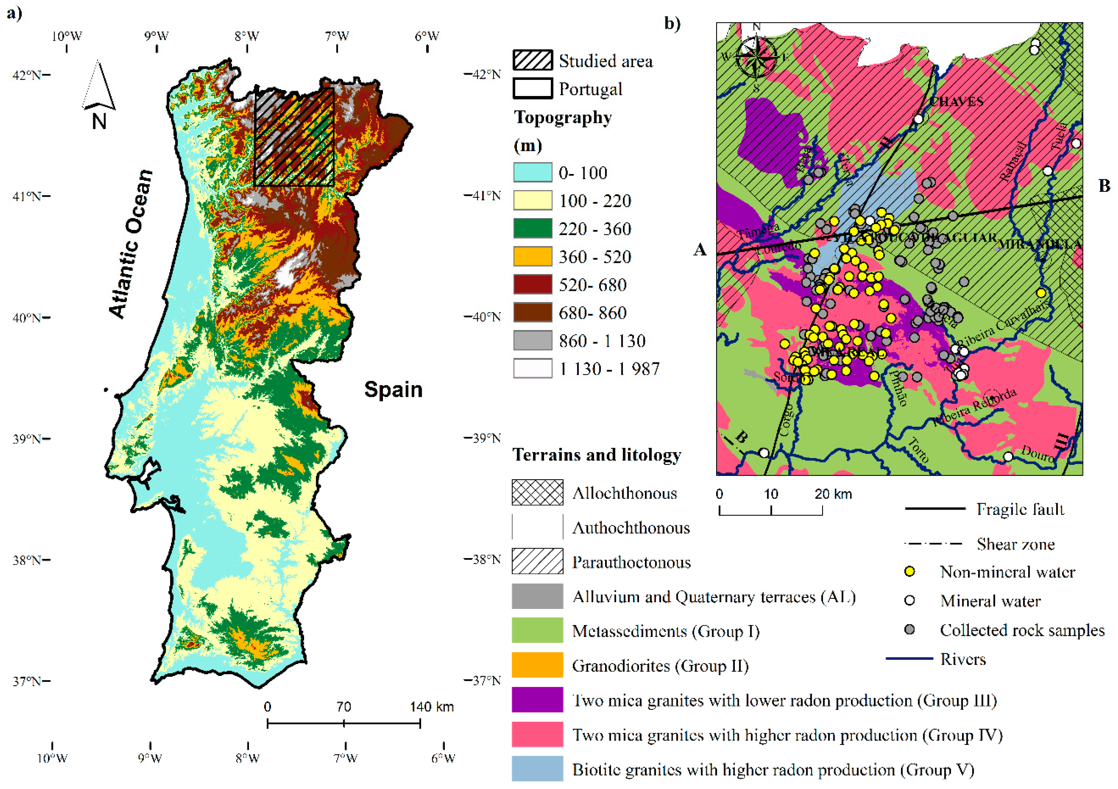
2.1. Location, Geomorphology, and Climate Study Area

The study area comprehends a sector of northern Portugal limited to the East and North by Spanish border and the West by the Atlantic coast (Figure 1a).

This region belongs to the Trás-os-Montes and Alto Douro province with topography contrasting among lowlands valley plains with the dendritic arrangement, craggy reliefs from the watershed boundary and nearby hillslopes. Therefore, altitudes in this region vary between 49 and 1507 m.a.s.l (Figure 1a), and the hillslopes comprise the north–northeast (NNE) to south–southwest (SSW) trending mountains of Gerês, Larouco, Barroso, and Marão-Alvão.

These undulated reliefs and fitted valleys by steep sides are located on the final section of the Tâmega river. The Tua river results from the junction of the Tuela and Rabaçal rivers. The main valleys of Tua river are bordered by Falperra, Padrela, Nogueira and Bornes mountains, with imposing granites and quartzite crests. These two main rivers bloom out in the Orense and Zamora provinces (Spain) while the course of water debouches into the Douro river. Essentially, the climate is moderately humid alternating between wet and dry periods. As a result of elevation differences, the rainfall ranges from 400 mm·year⁻¹ in the lowlands to 2700 mm·year⁻¹ in the highlands (30-years average; [45]). Natural recharge of the fissured aquifer system developed though rainfall across the saprolite layer and the underlying fracture network. The hydraulic flow occurs in local leptosols, fractured aquifers, and flows as a double porosity system though interflow and baseflow [46]. The natural flow discharge occurred mainly by fracture-artesian springs, boreholes, and dug wells.

2.2. Geology

The study region is located in the Autochthonous terrains of the Central Iberian Zone (CIZ), separated by Main Trás-os-Montes Thrust (MTMT; [47,48,49,50,51]) from two overlapping domains of the Galiza-Trás-os-Montes Zone (GTMZ): (a) the Parautochthonous terrains at the base and (b) Allochthonous domains at the top (Figure 1b; [52]). The metasediments arrangement into a single group was performed through its similar radiological identity. By contrast, granitoids were separated into different groups, being classified by their installation age and its rock’s ability to produce radon (Figure 1b). Several groups of granitoids occur in the study area, namely granodiorites of São Lourenço (Group II), two-mica granites with low-radon production (Group III), two-mica granites with high-radon production (Grupo IV), and biotite granites with high-radon production (Group V). The emplacement of these granitoids occurred during the ductile–fragile deformation phases (D3 and D4), between 321 and 290 Ma [53]. These Variscan granitoid outcrops in the metasedimentary formations of the Schist-Grauwacke Complex (Neoproterozoic-Lower Cambrian), Lower to Upper Ordovician, in the lower set of nappes Parautochthonous Thrust Complex (Silurian-Devonian) and Allochthonous Complex Domain with the installation during the Middle Devonian [54].

The tectonic depressions are significant relief forms, being related to the main regional tectonic accident called Penacova-Régua-Verín fault (PRVF). The movement along this geotectonic structure with a NNE–SSW direction produced tectonic hillslopes, which limit some depressions as a result of the maximum compression axis NW–SE in the Upper Miocene, causing left disconnections and push-up reliefs in the Alvão-Marão mountain [55]. For the evolution of drainage network, much contributed the Variscan heritage with the contrasts between the granitic massifs, the quartzite reliefs such as the Murça ridges, as well as the influence of late-Variscan fracturing network in contact with the fluvial courses [56].

3. Materials and Methods

3.1. Analytical Methods

3.1.1. Radiological Profile in Rocks

Given the substantial amount of radon production potential and emanation coefficient data collected in metasedimentary and granitic rocks (n = 119) from the studied area of Martins [57] and Martins et al. [58], the planning of radiological groundwater protection on the current study was performed only in a restricted area provided in Figure 1b. The emanation coefficient and radon production potential methodologies are widely described in Pereira et al. [59]. The radioactive isotopes of rocks namely, potassium (K₂O), uranium (U) and thorium (Th) were analyzed by gamma spectrometry with thallium-activated sodium iodide (NaI(Tl)) detector and 3-inch diameter, branded ORTEC, with samples placed inside a lead shield to protect from background radiation. A total of 119 representative samples was collected in metasedimentary (n = 50) and granitoids outcrops (n = 69). In general, these rocks samples present a low degree of physical alteration, with 500 g of weight previously milled in a grinder with a particle size less than 2 mm being collected. After grinding these rocks, samples are placed in Marinelli beakers with a volume of 0.2 L. After this preparation, the samples should remain at rest isotopic equilibrium, even before spectrometer measurements. The measurement time per sample used is 36,000 s corresponding to about 10 h of continuous measurements. To carry out a suitable calibration, standard measurements provided by the International Atomic Energy Agency (IAEA) were carried out under the same experimental conditions. Depending on the isotope analyzed and its activity, the uncertainties are variable, being estimated between 5% and 25% of the measured value. K₂O activity is directly measurable through ⁴⁰K occurring at the peak of 1460 keV, the U was measured through ²¹⁴Bi at the peak of 1764 keV, and Th through ²⁰⁸Tl at the 2614 keV peak. All peaks were observed with the right intensity and without any overlap.

3.1.2. Groundwater Sampling and Hydraulic Turnover Time Calculation

This groundwater radiological study was developed during summertime (July 2014) with 97 groundwater samples (springs, boreholes and dug wells) collected over a wide area of Trás-os-Montes and Alto Douro region. The groundwater collection sites were previously performed based on natural discharge, lithological variability, contact zones, intense fracturing, a radiometric map, and the presence of natural groundwater sources used for public supply. The radioisotope ²²²Rn sampling was previously carried out with the preparation of the water vessels that contain 12 mL of scintillation cocktail (Betaplate) in each one. In this selected collection sites, the geographical coordinates, capture type, date and time, electrical conductivity (μS·cm⁻¹), pH, and temperature (°C) were included in the field measurements. For the analyses of electrical conductivity and temperature we used a portable WTW LF320 conductivity meter and for pH we used a portable WTW pH320 pH meter. The following procedures for radiological analysis require the collection of 10 mL of groundwater into the vial. This process implies that the minimum of turbulence is developed to avoid air bubbles. After sealing the vial, the content should be shaken to mix the collected water with the Perkin-Elmer ^® scintillation cocktail. Radon gas is preferably concentrated in the organic phase, immediately below of cocktail level (double-phase method; [60]). The analytical procedures were performed in the Laboratory of Natural Radioactivity (LRN)–University of Coimbra, following the methods available in Pereira et al. [61]. Groundwater radon isotope was measured on the Perkin-Elmer^® Quantullus 1220 ultra-sensitive spectrometer with Liquid Scintillation Counting (LSC). In general, the estimated overall error is less than 15% of the measured values. To confines radon gas, teflon-coated polyethylene vials were used [62]. After three hours of sample resting, where the equilibrium between the radon and its short half-life progeny is restored, the groundwater sample is introduced into the spectrometer. Corrective action shall then be taken on the regular activities as a function of the elapsed time between the analysis and the harvest. Resting time efficiency was assessed by measuring several standard solutions of ²²⁶Ra after radon had reached the secular equilibrium of 21 days. The hydraulic turnover time (t, s) can be estimated through a combination of streamflow discharge rate (Q, m^–3·s^–1) and a1 and a3 constants retrieved from a scatter plot of ln(ΔQ/Δt) versus. ln(Q), as proposed by [63]:

$$\mathrm{t}=\frac{1.98}{\mathrm{Q}\sqrt{{\mathrm{a}}_1{\mathrm{a}}_3}}$$

(1)

where a1 and a3 correspond to intercept y values of straight lines with slope 1 and 3 representing the lower envelope to the scatter points. All data for the calculation of hydraulic turnover time are given in Table S3 of the Supplementary Materials.

In the absence of streamflow discharge rate and a1, a3 data for the calculation of hydraulic turnover time in the total collection points, only data related with Group V was removed from a study of Pacheco and Van der Weijden [37]. Some studies show the importance of applying several methods that evaluate and predict groundwater levels using artificial intelligence by neural network simulation [64,65,66,67] and dendrochronology [68]. On the other hand, another study developed by Alizadeh et al. [69] shows that it would be important to explore the river-flow-induced impacts in the performance of machine learning models applied for water quality-radiological parameters. For future studies, it is intended to explore and apply for this study region these previously mentioned methods. As the amount of radon depends on some features such as aquifer material, water–rock interaction, hydraulic turnover time, uranium content, etc. [5,31,70,71], it should be noted that local and intermediate flows circuits may contain high-radon concentrations, mainly due to its short time of water–rock interaction from the half-life of radon. As such, in radiological studies, it is crucial to relate the estimated spring’s turnover time and streamflow discharge rate with the radon contamination.

3.2. Hydrogeological Conceptual Model

Currently, some limitations are still recognized in the knowledge of the processes that control the radon emanation, as well as the transport mechanisms on geological materials. The radon emanation in rocks occurs when the disintegration of the radium atom leads to the generation of the radon atom, which being a gas can migrate for different natural systems. The porosity, grain size, and emanation coefficient control the permeability and subsequent radon mobility in the rocks. The crystalline rocks originate fractured aquifers with variable bedrock hydraulic properties (hydraulic conductivity and effective porosity), thus promoting the efficiency of the recharge rate compared to other types of rocks (Figure 2a).

The configurations in the hydrogeological framework during the radon transport in shallow and deep circuits are portrayed in Figure 2b. This conceptual model was used in this study, with the necessary adjustments and represents the typical flow systems of fractured rock aquifers that develop an exchange between shallow and deep groundwater and water–rock interaction. Precipitation accumulates in the saprolite horizon and flows through the fissured aquifer of interflow and baseflow, working as a double porosity system [46]. In this studied area, where the topography has a sharp relief, infiltrated water is also subject to lateral flows, and a parcel of it drains through the saprolite horizon, and shallow fractures ultimately emerging in springs, boreholes and dug wells.

The aquifer storage capacity and hydraulic turnover time are also crucial for radon transfer from rocks to the groundwater. It means, therefore, that in shallow hydraulic circuits with certain physical-chemical conditions (electric conductivity, temperature, and pH), the transfer of radon to the groundwater may occur, depending on a longer time of water-rock interaction. The hydraulic turnover time in hydrogeological systems are extremely variable and may occur over days up to thousands of years. In addition, in this conceptual model where the flow lines are represented, the sub-vertical fracture system allows three situations: (a) local flow system (green flow lines), (b) intermediate flow system (yellow flow lines) and (c) regional flow system (red flow lines; Figure 2b).

On the other hand, there may be a mixture of water circuits coming from different depths (springs a, b, and c of the conceptual model; Figure 2b). However, to validate this previous hypothesis, there is no discharge rate for all water collection points to compute the turnover time. Radon gas may thus become a hydrogeological marker for aquifer systems with relatively short flow distances. Since the radon half-life is only 3.8 days, after about 20 days the radon concentration generally decreases considerably to the point of not being analytically detectable [72]. Furthermore, the radon levels in mineral and non-mineral waters can be higher if the system of water collection points has an open water circuit (e.g., without water tap or closed borehole) which, associated with high recharge, may bring more elevated amounts of dissolved radioactive minerals to the surface [9].

Figure 2. A hydrogeological conceptual model for radon contamination in groundwater of the studied region. (a) Geologic section profile with tectonic structures like thrust faults, faults and shear zones and fault-joint/fault-lineament types faults; (b) main tectonic structures with a microscopic overview of radon transfer from metasedimentary and granitic rocks to groundwater. A detailed description of model premises is provided in Section 3.2.

Figure 2. A hydrogeological conceptual model for radon contamination in groundwater of the studied region. (a) Geologic section profile with tectonic structures like thrust faults, faults and shear zones and fault-joint/fault-lineament types faults; (b) main tectonic structures with a microscopic overview of radon transfer from metasedimentary and granitic rocks to groundwater. A detailed description of model premises is provided in Section 3.2.

The geogenic and hydrogeological conditions are essential for the design of this conceptual model of water–rock interaction, displaying a radon transfer from the surrounding rocks to mineral and non-mineral water. The dynamics of interaction between all these features described above is extremely complex, and it is particularly challenging to establish coherent models to explain the radon transfer rate from rocks to the groundwater. For this purpose, the application of this conceptual model through the combination of hierarchic agglomerative clustering (HAC) and PLS-PM analysis may help to demystify this controversial issue mainly due to the study of several involved processes in water-rock interaction.

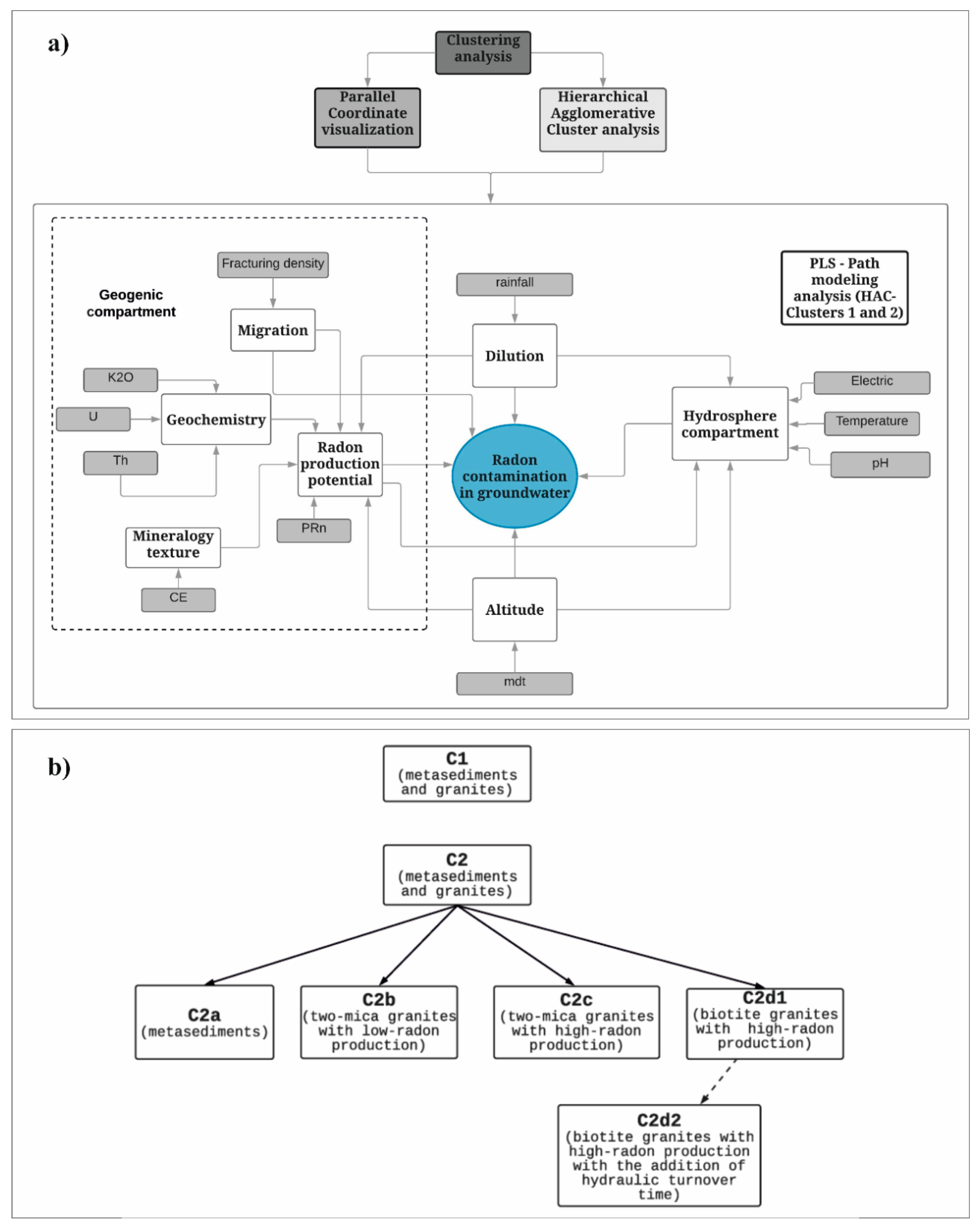
3.3. Technical Workflow

This scientific workflow was prepared to estimate the groundwater radon contamination in this study region. This workflow is composed of three interconnected modules (Figure 3a): (1) the HAC, which uses a graphical representation of hierarchical clusters (dendrogram) that ensure the grouping of the database through dissimilarities between objects; (2) the parallel coordinates visualization (PCV) to describe groups according to measured variables, and (3) the PLS-PM module which define connections between established latent variables (LV).

The main purpose of the PLS-PM module is verifying if the radon contamination in groundwater can be related to the (a) geogenic compartment, (b) hydrosphere compartment, (c) altitude, and (d) dilution. Firstly, in the geogenic compartment occurs the interaction of several features (geochemistry, mineralogy texture, and migration) which may influence the radon amount available for transport in rocks (PRN, radon production potential). The geochemical profile is represented by potassium, uranium and thorium contents (K₂O, U, and Th, respectively), the mineralogy texture that characterizes the rock’s ability to release radon (emanation coefficient), and fracturing density. Secondly, the hydrosphere compartment implies the action of some physical-chemical properties (electric conductivity, temperature, and pH). Thirdly, this PLS-PM analysis also explores the effect of dilution (rainfall recharge) in the radon production potential, radon contamination in groundwater and hydrosphere compartment. Besides, it is also essential to understand the interaction between altitude (digital terrain model) and the latent variables described previously. Subsequently, once the geogenic component is crucial for the description of the radiological profile of the rocks, the cluster C2 was subject to the lithological reorganization (Figure 3b). A more detailed description of this reorganization will be further discussed in Section 4.

3.3.1. Clustering Analysis (Hierarchical Agglomerative Cluster (HAC) Analysis and Parallel Coordinate Visualization (PCV))

The entire dataset used for HAC analysis and PCV has been extracted from physical-chemical, climate, topographic and radiological conditions depicted in Tables S1 and S2 of Supplementary Materials. The HAC and PCV are two graphical users interface tools, available in Excel using the XLSTAT statistical software. The HAC is one of the most popular clustering methods that portrays the dissimilarities between objects to be grouped, resulting in a dendrogram, which shows the following data grouping with a suitable number of clusters. The process starts when a specific number of objects minimize the agglomeration criterion, creating a cluster that comprises them. The dissimilarity between these clusters is computed using the agglomeration criterion, and this process only ends until all objects have been clustered. These successive clustering operations produce a binary clustering tree that represents a hierarchy of partitions, where it is possible to choose a partition at a given level through some objective criteria. For this work, the proximity type used was the dissimilarity through the Euclidean distance, also applying the ward’s agglomeration method with a truncation of four clusters. Ward’s method was used to create groups, where the variance within the groups is minimized. According to Hands and Erit [72], Blashfield et al. [73] e Mooi and Sarstedt [74], the ward’s method performed significantly better than other clustering procedures. The PCV visualization method is a useful tool for HAC data analysis to describe groups using variables. Thus, the goal of the PCV plot is to comprise what features (altitude, precipitation, electric conductivity, temperature, pH and ²²²Rn in groundwater) may influence the dissimilarity between each cluster generated by HAC analysis.

3.3.2. Partial Least Squares-Path Modeling (PLS-PM)

In the last decades, partial least squares developed by Wold [75,76] was the most effective advanced statistical analysis techniques that emerged in social sciences, mainly due to constant increasingly data. In the present study, PLS-PM was applied in the Smart-PLS Software [77], and it was used as a formative model because measured variables are viewed as causes of LV [78].

The initial planning workflow comprehends a statistical modeling technique that established causal connection paths among blocks of variables called latent variables (LV), which further linked to measured variables (MV). Path coefficients represent the effect of exogenous on endogenous latent variables and are computed through links among LV, while the connections between LV and MV are quantified by weights [79]. For each regression in this structural model, the coefficient of determination (R²) plays an important role, representing the amount of variance in the latent dependent variable (endogenous) explained by its independent latent variable (exogenous). The PLS-PM models may be formative or reflective (or rarely, mixed). A reflective path model is characterized by a path diagram with causal arrows, which start in a latent variable (factor) and end up in the measured indicator variables. In the formative path model, the arrow senses are reversed [80], being the model preferentially used in several studies (Figure 4a; [81]).

The measured score of an LV (LV_j; Figure 4b; Equation (1)) is the weighted sum of X_i scores [82], and the predicted score of an endogenous LV (e.g., LV_p,c in Figure 4b; Equation (2)) is the weighted sum of all exogenous latent variables and path coefficients (pc):

$${\mathrm{LV}}_{\mathrm{j}}={\displaystyle \sum }_{\mathrm{i}-1}^{\mathrm{n}}\left({\mathrm{X}}_{\mathrm{i}\times {\mathrm{W}}_{\mathrm{i}}}\right)$$

(2)

$${\mathrm{LV}}_{\mathrm{p},\mathrm{c}}={\mathrm{LV}}_{\mathrm{A}}\times {\mathrm{pc}}_{\mathrm{ac}}+{\mathrm{LV}}_{\mathrm{B}}\times {\mathrm{pc}}_{\mathrm{bc}}$$

(3)

All information about the sources and complete dataset of measured and latent variables are depicted in

Table 1. Sources of information and list of measured variables used as a source data for partial least squares-path modeling (PLS-PM). This table contains the identification of variables, their measurements units, and description. The n values represent the number of sites used in the interpolation of variables that were measured solely at specific locations (see locations in Figure 1b) Websites was assessed in February 2017. Symbol description (institution names in Portuguese): SNIRH—Sistema Nacional de Informação em Recursos Hídricos; DGT—Direção Geral do Território.

Compartment Type		Measured Variable	n	HAC Classes				Units	Description	Source
				1	2	3	4
Water 222Rn	222Rn		97	x	x	x	x	Bq·L−1	Radon potential data in groundwater from 97 monitoring
Geogenic compartment	Geochemistry	K2O	119	x	x	x	x	%	Measured radioactive potassium in 119 samples of rocks and soils of the studied area using a portable spectrometer
		U	119	x	x	x	x	ppm	Measured radioactive uranium in 119 samples of rocks and soils of the studied area
		Th	119	x	x	x	x	ppm	Measured radioactive thorium in 119 samples of rocks and soils of the studied area
	Mineralogy texture	CE	119	x	x	x	x	%	Mineralogy texture in 119 samples of rocks (emanation coefficient)	[57]
	Radon production potential	PRN	119	x	x	x	x	Bq·m−3·h−1	Radon production potential in 119 samples of rocks of the studied area	[57]
Hydrosphere compartment	Electric conductivity		97	x	x	x	x	µS·cm−1	Electric conductivity data of 97 monitoring stations
	Temperature		97	x	x	x	x	°C	Temperature data of 97 monitoring stations
	pH		97	x	x	x	x	dimensionless	pH data of 97 monitoring stations
Altitude	mdt		97	x	x	x	x	m	Topography obtained from analysis of a digital elevation model (DEM)	DGT
Migration	Fracturing density		*	x	x	x	x	km·km−2	Possible migration of radon by fracturing density in rocks from entire studied area	[53]
Dilution	Rainfall		*	x	x	x	x	mm·year−1	Annual precipitation that may promote some dilution of radon in groundwater	Portuguese information on Water Resources

* These variables were used from shapefile and raster files.

. For this path modeling, all weights and path coefficients were initially set to 1, consider the default value for this software. The final values are being reached after a maximum number of 300 iterations that usually ensures the convergence model and the highest values of R² for endogenous latent variables [83]. A well-fitting formative measurement model should not display excessive multicollinearity of indicator variables in the set for any given formative modeled factor [79]. Nonetheless, since formative models embody a form of ordinary least squares (OLS) regression, the usual regression test for multicollinearity problems may be applied.

In this type of formative modeling, the multicollinearity may be a problem if the variance inflation factor (VIF) exceeds 5. Therefore, when R-squared for a formative factor is less than 0.80, multicollinearity is not a problem by the criteria of VIF > 5.

Hair et al. [79], suggest that formative factors flagged for high multicollinearity by VIF tests must be dropped from the model or otherwise operationalized. Nevertheless, Garson [84] disagrees with this suggestion, since it is true that multicollinearity among the indicators for a formative factor inflates standard errors and makes an assessment of the relative importance of the independent variables unreliable, such high multicollinearity does not affect the efficiency of the regression estimates. Instead, this author mentioned above considers that some emphasis should be given to the items for a formative factor, including the coverage of all constituent dimensions.

3.4. Dataset Preparation

The radiological analysis in rocks, groundwater, and hydraulic turnover time dataset are all provided in Tables S1–S3 of the Supplementary Materials in three separate Excel files. Other Excel files for PLS-PM dataset and data modeling results with correlation matrix, external and internal VIFs are depicted in Tables S4–S29. The Geographic data are represented as figures embedded along with the current text. They were prepared using ArcMap [85], a computer package increasingly used in many hydrologic and environmental studies [86,87,88,89,90,91,92,93,94,95,96,97,98,99,100,101]. The complete summary dataset with information sources is depicted in Table 1 and Figure 5a–g. In Figure 5a–g, the maps of measured variables were prepared with ArcMap’s kriging geostatistical tool and the Zonal Statistics as Table tool to obtain the average value for each water collection point. These average values were subsequently exported to the Excel worksheet for each cluster with a specific geology group (Tables S4, S8, S12, S16, S20, and S24) to be used in the Smart PLS-PM software [77].

The average value for each interpolated variable was computed for each water collection point using a buffer of 500 m. Some variables were collected as raster files from the sources available online (Figure 5a,b; Table 1), namely precipitation and fracturing density. In these cases, a buffer of 500 m was also generated, and the ZST tool was applied directly to the measured values. It is also important to mention that only 8 collection sites used for PLS-PM analysis were excluded from clusters C1 and C2 (n = 72) because they were located outside of the border area of the respective interpolated rasters. The number of measured sites is depicted in Table 1, and the interpolated locations that overlap to the water collection points are illustrated in Figure 5a–g.

4. Results

Given the substantial amount of physical-chemical and radiological groundwater data collected from Trás-os-Montes and Alto Douro region, the protection planning of drinking water is extremely important to ensure public health.

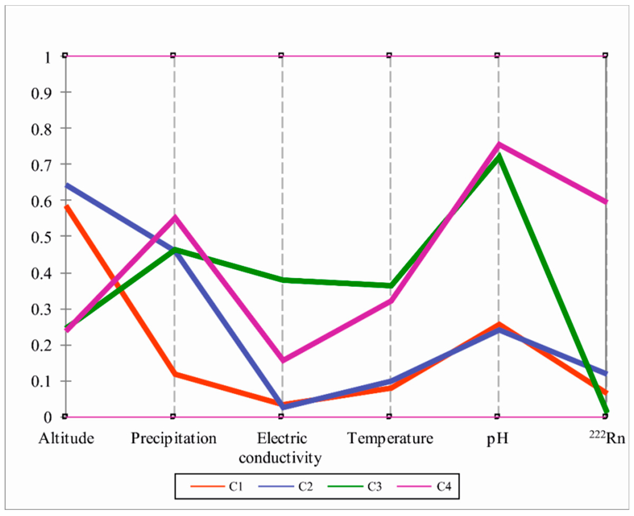
4.1. Clustering Analysis

The results of the HAC analysis (n = 97) are summarized in

Table 2. Descriptive statistics for climatic, topographic, and physical-chemical hydrologic parameters of each HCA cluster.

Id_HAC Classes	Statistics Criteria	Altitude (m)	Precipitation (mm·year−1)	Electric Conductivity (µS·cm−1)	Temperature (°C)	pH	222Rn (Bq·L−1)
Class 1 (n = 15)	µ ± σ	657.3 ± 176.1	670.4 ± 102.4	109.8 ± 86.8	14.3 ± 1.7	5.7± 0.4	245.9 ± 230.7
	Med	602.0	657.9	67.5	14.7	5.9	111.6
	CV	0.3	0.2	0.8	0.1	0.1	0.9
	Min.–Max.	440–1053.0	453.6–833.3	24.7–274.0	11.5–16.8	5.0–6.5	37.4–642.1
Class 2 (n = 65)	µ ± σ	715.4 ± 169.3	1291.6 ± 221.1	88.8 ± 85.9	15.2 ± 2.6	5.7± 0.4	439.3 ± 380.5
	Med	725.0	1286.9	51.6	15.0	5.6	342.3
	CV	0.2	0.2	1.0	0.2	0.1	0.9
	Min.–Max.	306.0–1078.0	901.9–2275.4	18.1–343.0	10.3–22.3	4.7–6.9	9.7–1520.7
Class 3 (n = 11)	µ ± σ	305.4 ± 157.5	1298.4 ± 316.4	973.2 ± 725.6	28.0 ± 13.0	7.7 ± 1.0	49.8 ± 46.7
	Med	284.0	1341.8	728.0	22.4	7.9	38.9
	CV	0.5	0.2	0.7	0.5	0.1	0.9
	Min. –Max.	54.0–594.0	538.0–1803.6	335.0–2520.0	15.4–58.8	6.1–8.9	0.6–172.2
Class 4 (n = 6)	µ ± σ	297.8 ± 90.4	1463.1 ± 122.6	413.8 ± 39.0	26.0 ± 4.2	7.9 ± 0.4	2196.4 ± 802.0
	Med	311.5	1456.6	408.0	27.0	7.9	1949.3
	CV	0.3	0.1	0.1	0.2	0.1	0.4
	Min.–Max.	163.0–396.0	1249.6–1642.1	364.0–485.0	17.8–31.1	7.1–8.3	1419.1–3687.7

Symbols: ID is the identification code of the collecting site.

for physical-chemical, climatic, topographic, and radiological features, as well as in the dendrogram of Figure 6a–b. According to the PCV procedure, when the mean lines are activated, the XLSTAT displays for each cluster a line with the mean of the multiple measured variables. This means, therefore, that when the rescale option is activated, it facilitates the visualization of multiple measured variables distribution for each cluster.

Through the impact of the dissimilarity degree in the total dataset, four different clusters were generated. Two profiles with two homogeneous clusters for mineral water (C3 and C4) and non-mineral water (C1 and C2, Figure 6b) are visible.

An Excel worksheet comprising n rows and p columns was only prepared for two homogeneous clusters of HAC analysis (Cluster 1 and 2) to be used as input data for Smart-PLS, where n represents the water collection points and p the number of measured and interpolated variables. The value of n was set to 12 in cluster 1 and 60 in cluster 2. These homogeneous clusters represent only non-mineral waters, distinguishing themselves through geology.

The water collection points of C1 cluster are composed mainly of metasedimentary rocks (Group I), whereas in C2 outcrops mostly on granitoids (Groups III, IV, and V). The remaining clusters produced by the HAC analysis (Clusters 3 and 4) representing mineral waters which were not included in the PLS-PM modeling due to an insufficient data set (n < 10). Since some features are unknown in the groundwater sampling sites, the use of the kriging interpolation tool becomes crucial for a consistent dataset preparation (Figure 5c–g). Other interpolation methods were tested (Inverse distance weighted and topo to raster). Hence, the kriging tool proved to be more robust and efficient in the present case, due to the sparse available data embedded in most of the measured variables.

The HAC results represented in a PCV plot were depicted in Figure 7, to explain which features influenced the established categorization. This projection displays two typical patterns, highlighting the importance of precipitation, pH and ²²²Rn values (Med = 1456.6 mm. year⁻¹, 7.9 and 1949.3 Bq.L⁻¹, respectively; Figure 7; Table 2) in mineral water (cluster C4), remaining high altitude values (Med = 725.0 m; Figure 7; Table 2) for non-mineral water (cluster C2).

The collected water sites used for human consumption are inserted in clusters C1 and C2, and it is essential to highlight the maximum value of altitude obtained for each of these clusters (Max = 1053.0 and 1078.0 Bq·L⁻¹; Table 2).

In most clusters (C1, C2, and C3), the variability was significant, particularly with regards to electric conductivity and ²²²Rn concentration; however, the altitude and pH features have a higher variation coefficient or close to 50% only for C3 (Table 2). The variability was particularly crucial in ²²²Rn concentration for these three clusters, wherein the variation coefficient was the highest percentage (90%; Table 2), although the electric conductivity followed a similar pattern of variation with ²²²Rn concentration (Table 2).

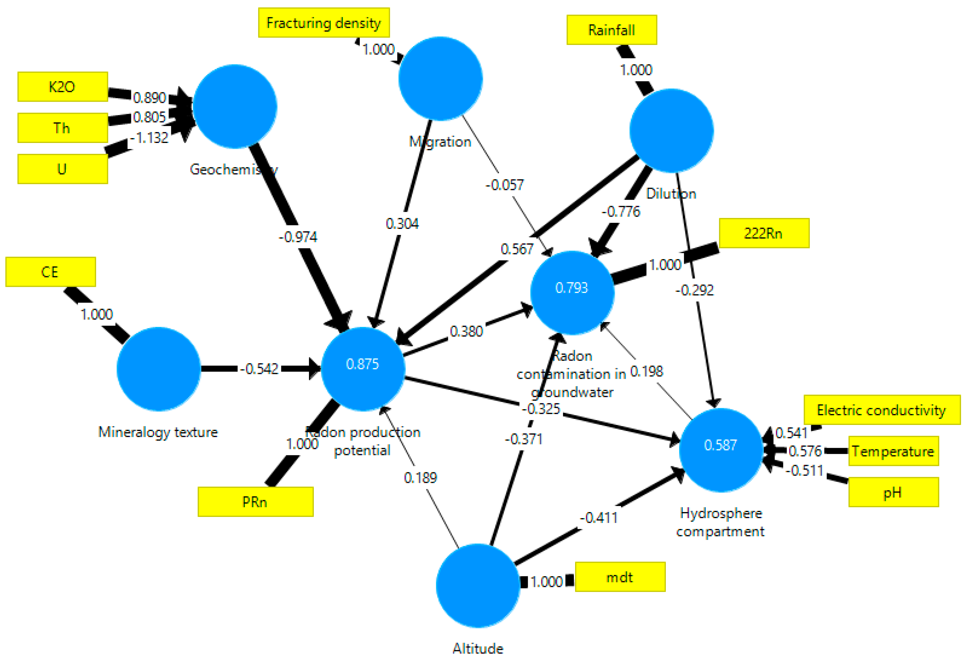
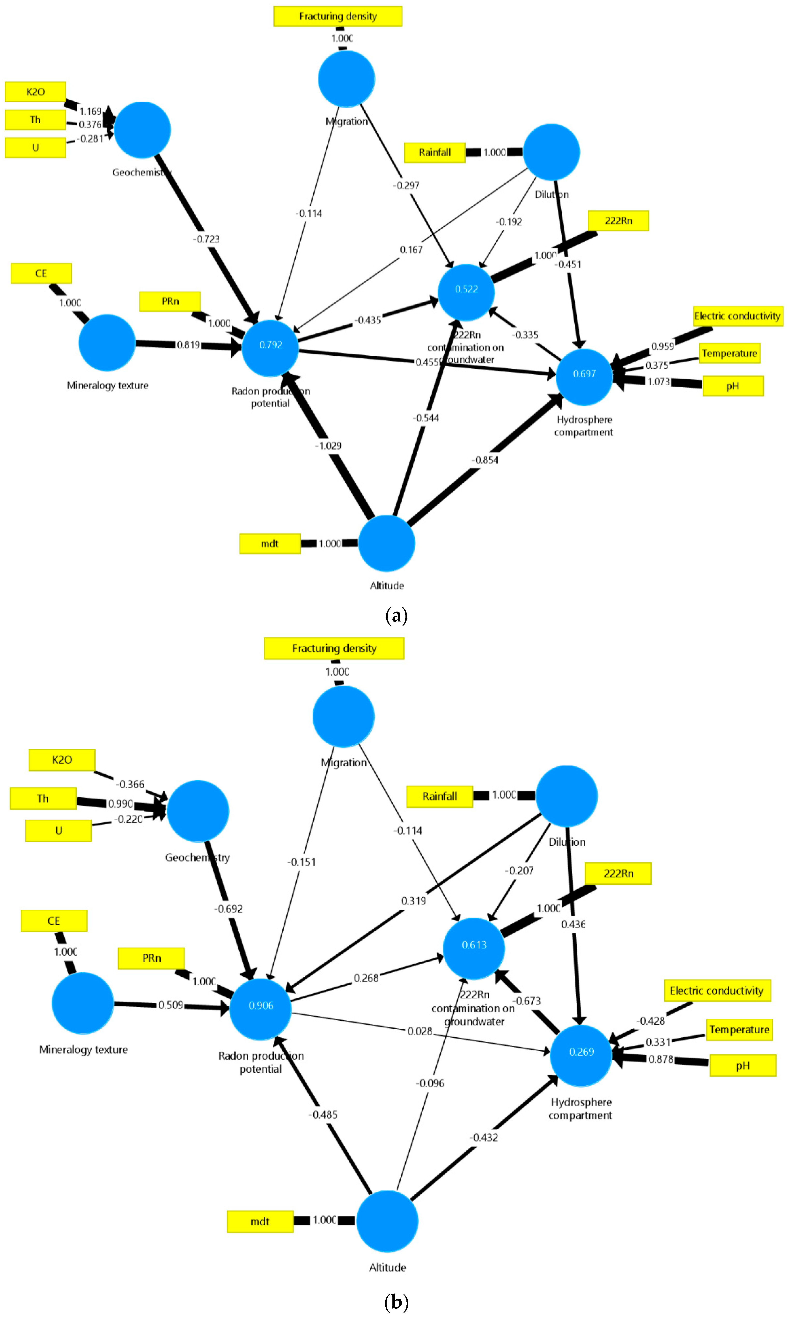
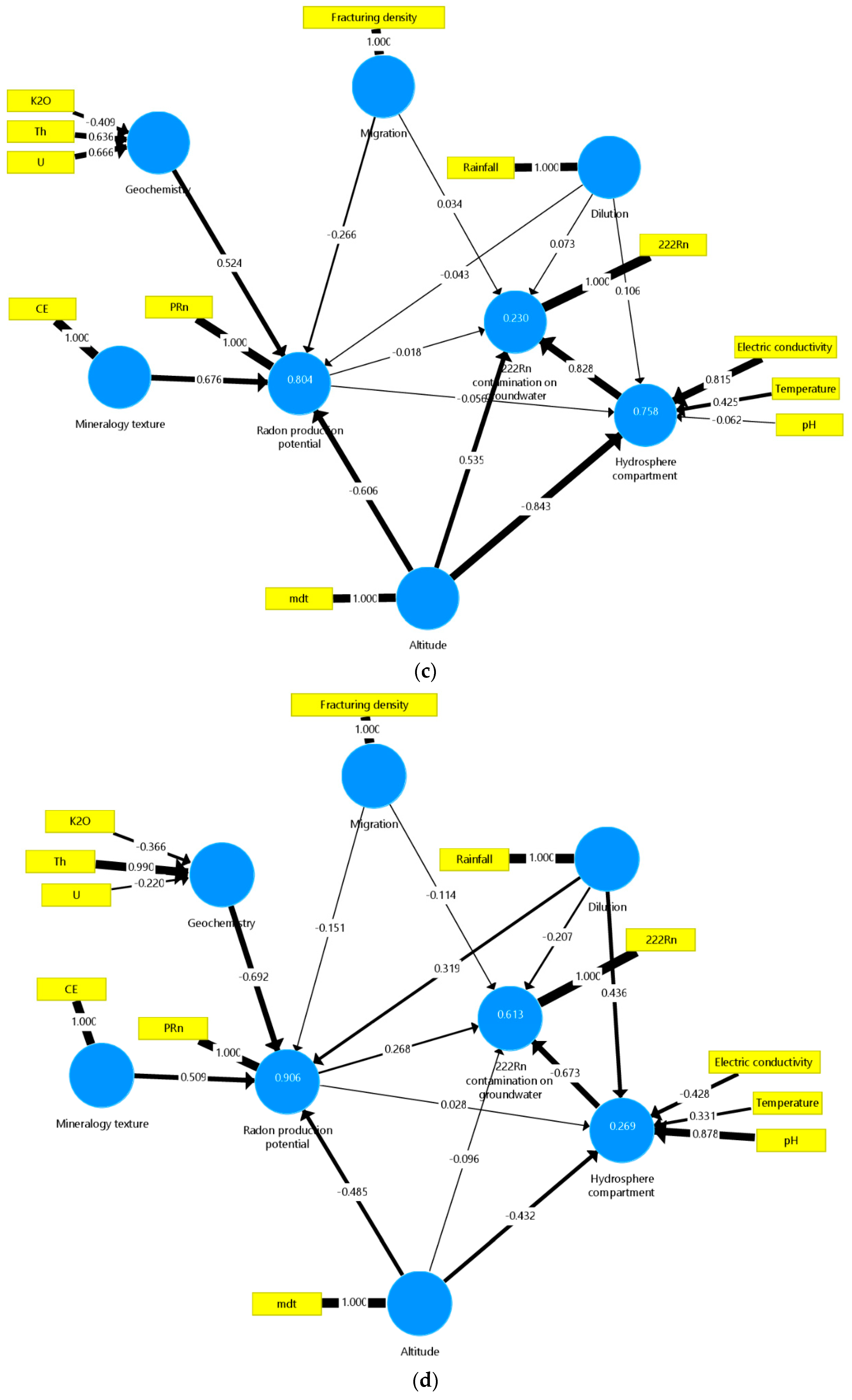
4.2. Partial Least Squares-Path Modeling

The PLS-PM of all computed and measured variables are represented in the maps of Figure 8, Figure 9 and Figure 10, where the links, path coefficients, and weights between latent, sub-latent, and measured variables are determined. The spatial measurement distributions are indicated in Figure 1b, from which the Excel worksheet was prepared to source PLS-PM data.

The application of PLS-PM to cluster datasets C1 and C2 (Tables S4 and S8) followed a three-step procedure: (1) in the first step all structural inner and outer model were used in the statistical model being linked to a three endogenous latent variables called “Radon contamination in groundwater—RN” and two sub-latent variables called “radon production potential—PRN” and “Hydrosphere compartment—HC”. Five exogenous latent variables are called “ Mineralogy texture–M”, “Geochemistry—G”, “Migration—M”, “Dilution—D” and “Altitude—A”; (2) in second step, since the R² of latent and sub-latent variables obtained for cluster C2 were low due mainly to the high radiological heterogeneity of granites, it was performed a refined analysis according to several types of granites (Group III, Group IV and finally Group V); (3) finally as in the third refinement analysis (Group V), R-squared was also low, it was decided the exclusive addition of hydraulic turnover time. All the equations generated through PLS-PM analysis for each model are depicted in

Table 3. Equations developed by PLS-PM models to represent the relationships between measured, exogenous, and endogenous latent variables.

Line	Model	Equation
1	C1	PRN = −0.542MT − 0.974G + 0.304M + 0.567D + 0.189A
2	C1	HC = −0.292D − 0.325PRN − 0.411A
3	C1	RN = 0.380PRN − 0.057M − 0.776D + 0.198HC − 0.371A
4	C2a	PRN = 0.819MT − 0.723G ± 0.114M + 0.167D − 1.029A
5	C2a	HC = −0.451D + 0.455PRN − 0.854A
6	C2a	RN = −0.435PRN − 0.297M − 0.192D − 0.335HC − 0.544A
7	C2b	PRN = 0.509MT − 0.692G − 0.151M + 0.319D − 0.485A
8	C2b	HC = 0.436D + 0.028PRN − 0.432A
9	C2b	RN = 0.268 PRN − 0.114M − 0.207D − 0.673HC − 0.096A
10	C2c	PRN = 0.676MT + 0.524G − 0.266M − 0.043D − 0.606A
11	C2c	HC = 0.106D − 0.056PRN − 0.843A
12	C2d1	PRN = 0.426MT + 1.234G − 0.178M − 0.555D + 0.236A
13	C2d1	HC = 0.821D − 0.413PRN − 0.180A
14	C2d2	PRN = 0.485MT + 0.822G − 0.394M − 0.580 + 0.265A
15	C2d2	HC = 0.759D + 0.480RN − 0.572A
16	C2d2	RN = 0.041 PRN + 0.545M − 0.553D + 1.380HC + 0.516A

. Depending on the model, the variance inflation factors were computed to detect multi-collinearity between measured variables (see Tables S6, S7, S10, S11, S14, S15, S18, S19, S22, S23, S26 and S29 of the Supplementary Materials). If two or more variables were collinear, it must have selected one and discarded the others to prevent the computed unpredictable weights [84].

4.2.1. Cluster C1 Composed by Metasediments and Granites (n = 12)

The variance explained by the cluster C1 model (Figure 8) is high for the endogenous latent variables PRN (R² = 0.875) and RN (R² = 0.793) and medium for HC (R² = 0.587). In line 1 of Table 3 is expressed the direct influence of exogenous latent variables like mineralogy texture (MT), geochemistry (G), migration (M), dilution (D) and altitude (A) on endogenous latent variable radon production potential (PRN; see general information in Equation (3); Table 3). On the same model, in line 2 of Table 3 is represented the direct influence of exogenous latent variables like dilution (D), radon production potential (PRN) and altitude (A) on the hydrosphere compartment (HC; Table 3). Finally, in line 3 of Table 3 is expressed the direct influence of latent variables PRN, M, D, HC, and A on groundwater radon contamination (RN; Table 3):

Figure 8. Diagrammatic representation of PLS-PM complete models for cluster C1 composed mainly by metasediments. The circles represent the latent variables, and the rectangles are the formation variables (see description in Table 1), the arrows characterize the links between the formation and associated latent variable, as well as among related latent variables, while arrow labels are weights and path coefficients that quantify those links. Please consult the caption of Figure 4 for additional information.

Figure 8. Diagrammatic representation of PLS-PM complete models for cluster C1 composed mainly by metasediments. The circles represent the latent variables, and the rectangles are the formation variables (see description in Table 1), the arrows characterize the links between the formation and associated latent variable, as well as among related latent variables, while arrow labels are weights and path coefficients that quantify those links. Please consult the caption of Figure 4 for additional information.

The most important measured values (w > 0.5) of latent variable geochemistry are potassium (w = 0.890) and thorium contents (w = 0.805). However, for latent variable hydrosphere compartment, the most measured variables are the electric conductivity (w = 0.541) and temperature (w = 0.576). The radon production potential has a more pronounced effect (w = 0.380) on radon contamination in groundwater than the remaining latent variables (Figure 8). When measured scores (Equation (2)) of latent variable radon contamination in groundwater are compared to corresponding predicted scores (Equation (3)), the following relationship is obtained: RNp = 0.793 RNm, which means a reduced deviation between measured and predicted scores. Moreover, all hypothesized path relationships are statistically significant, except for the standardized path coefficient between migration and radon contamination in groundwater, because its normalized path coefficient (pc = −0.057) is lower than 0.1 [81]. In general, the PLS results for cluster 1 are reliable because coefficients of determination of endogenous latent variables are medium to high (>0.5) and path coefficients with their signs expose the impact of exogenous on endogenous latent variables (this issue will be further discussed in Section 5). In general, for all measured parameters, the values were distributed over a wide range. However, this trend was different for precipitation, temperature, pH, K₂O, and Th (

Table 4. Descriptive statistics for climatic, topographic, physical-chemical water properties, and geogenic parameters of each cluster used for PLS-PM, including the segmentation performed on the C2 cluster based on the granite type.

Id_HAC	Statistics Criteria	Altitude (m)	Precipitation (mm·year−1)	Electric Conductivity (µS·cm−1)	Temperature (°C)	pH	222Rn (Bq·L−1)	PRn (Bq·m−3·h−1)	CE	K2O (%)	Th (ppm)	U (ppm)	Fracturing Density (km·km−2)	Turnover Time (years)
Cluster 1 (n = 12)	µ ± σ	707.3 ± 162.0	689.3 ± 93.9	76.4 ± 59.0	14.1 ± 1.7	5.7± 0.5	285.1 ± 242.6	165.6 ± 55.6	0.14 ± 0.06	5.0 ± 0.6	15.4 ± 1.4	7.4 ± 2.6	1.7 ± 0.7
	Med	670.5	677.7	53.5	14.4	5.6	216.0	152.2	0.13	5.0	15.0	8.4	1.7
	CV	0.2	0.1	0.8	0.1	0.1	0.9	0.3	0.39	0.1	0.1	0.3	0.4
	Min.–Max.	495.0–1053.0	581.1–833.3	24.7–235	11.5–16.8	5.0–6.5	37.0–642.0	100.3–313.2	0.06–0.22	4.2–5.7	13.4–18.4	2.7–11.3	0.4–2.7
Cluster 2 (n = 60)	µ ± σ	731.7 ± 147.4	1291.6 ± 221.1	85.4 ± 84.9	15.2 ± 2.6	5.7± 0.4	457.6 ± 387.3	189.3 ± 63.5	0.13 ± 0.04	5.2 ± 0.3	15.0 ± 0.9	8.3 ± 2.2	1.7 ± 0.7
	Med	734.5	1287.6	48.8	15.0	5.6	387.0	173.7	0.13	5.3	14.9	8.5	1.7
	CV	0.2	0.2	1.0	0.2	0.1	0.8	0.3	0.28	0.1	0.1	0.3	0.4
	Min.–Max.	306.0–1078.0	901.9–2275.4	18.1–343.0	10.3–22.3	4.7–6.9	14.0–1521.0	95.7–397.0	0.04–0.21	4.4–5.9	12.5–18.9	2.9–13.6	0.1–3.4
Cluster 2a (Group I) (n = 11)	µ ± σ	677.3 ± 183.6	1339.5 ± 347.5	120.7 ± 113.6	15.8 ± 3.0	5.6 ± 0.4	273.0 ± 298.4	159.9 ± 36.2	0.13 ± 0.04	5.1 ± 0.4	14.9 ± 0.5	6.9 ± 2.6	2.2 ± 0.5
	Med	701.0	1322.8	56.0	15.3	5.6	137.0	153.2	0.12	5.3	14.9	7.7	2.1
	CV	0.3	0.3	0.9	0.2	0.1	1.1	0.2	0.33	0.1	0.0	0.4	0.2
	Min.–Max.	413.0–970.0	933.0–2275.4	28.7–330.0	12.1–22.3	4.7–6.3	14–1013.0	95.7–234.2	0.04–0.21	4.4–5.7	14.2–16.0	2.9–12.2	1.5–3.2
Cluster 2b (Group III) (n = 17)	µ ± σ	751.1 ± 74.5	1292.3 ± 232.3	74.1 ± 67.8	15.6 ± 2.6	5.6 ± 0.4	567.9 ± 444.1	165.1 ± 31.9	0.11 ± 0.02	5.3 ± 0.2	15.0 ± 1.4	9.8 ± 0.2	1.7 ± 0.8
	Med	732.0	1286.9	49.8	15.1	5.5	389.9	157.3	0.11	5.3	14.9	9.8	1.5
	CV	0.1	0.2	0.9	0.2	0.1	0.8	0.2	0.22	0.0	0.1	0.2	0.5
	Min.–Max.	628.0–879.0	901.9–1911.0	18.1–250.0	12.3–20.8	5.1–6.6	116.4–1520.7	108.6–213.5	0.07–0.14	4.8–5.9	12.5–18.9	4.8–13.6	0.6–3.4
Cluster 2c (Group IV) (n = 20)	µ ± σ	729.8 ± 171.1	1261.9 ± 136	86.6 ± 92.2	14.7 ± 2.7	5.6 ± 0.4	594.2 ± 368.2	190.8 ± 75.2	0.13 ± 0.03	5.4 ± 0.2	14.8 ± 0.6	7.9 ± 1.4	1.8 ± 0.8
	Med	748.0	1251.1	34.5	14.6	5.5	588.5	166.1	0.12	5.4	14.8	7.8	1.9
	CV	0.2	0.1	1.1	0.2	0.1	0.6	0.4	0.24	0.0	0.0	0.2	0.4
	Min.–Max.	434.0–1035.0	1037.8–1553.2	19.1–343.0	10.3–21.3	5.0–6.7	31.0–1385.0	136.1–397.0	0.09–0.18	4.8–5.8	13.7–16.1	4.2–9.6	0.1–3.3
Cluster 2d (Group V) (n = 12)	µ ± σ	757.2 ± 130.9	1280.9 ± 165.9	67.1 ± 42.9	14.6 ± 1.9	6.0 ± 0.3	242.9 ± 193.8	248.0 ± 54.9	0.17 ± 0.02	4.8 ± 0.2	15.3 ± 0.7	8.1 ± 1.6	1.3 ± 0.5	16.1 ± 21.6
	Med	724.5	1286.9	54.6	14.8	6.0	189.5	240.3	0.17	4.8	15.2	8.4	1.2	7.2
	CV	0.2	0.1	0.6	0.1	0.1	0.8	0.2	0.13	0.0	0.0	0.2	0.4	1.3
	Min.–Max.	478.0–1078.0	1045.3–1573.9	21.2–164.0	11.4–17.8	5.6–6.9	46.0–749.0	163.0–344.5	0.14–0.21	4.6–5.3	14.2–16.9	5.3–10.7	0.8–2.7	1.9–71.2

Symbols: ID is the identification code of the collecting site; t is the turnover time of spring water (Equation (1)).

).

4.2.2. Cluster C2 Composed by Metasediments and Granites (n = 60)

The variances explained by the C2 structural model (Figure 9) are extremely low for radon contamination in groundwater (R² = 0.070). These results are not consistent because it is unlikely that all exogenous latent variables explain only less than 1% of radon contamination in groundwater. This incongruence is expected because this cluster is represented by several types of rocks, namely metasediments and granites with different radiological profiles. In this scenario, this cluster should not be applied singly in the PLS-PM model. On the contrary, it must be added separately in four other clusters composed by Group I, (C2a) Group III (C2b), Group IV (C2c) and finally Group V (C2d; Figure 10a–e). Regarding ²²²Rn activity, values ranged between 14 to 1521 Bq·L⁻¹ (Table 4), and the precipitation is also extremely variable, ranging from 902 to 2275 mm·year⁻¹ (Table 4).

Figure 9. Diagrammatic representation of PLS-PM complete models for cluster C2 composed by different groups of rocks from the studied region.

Figure 9. Diagrammatic representation of PLS-PM complete models for cluster C2 composed by different groups of rocks from the studied region.

(a) Cluster C2a composed by metasediments—(Group I)

The variances explained by the C2a cluster model (Figure 10a) is high for the endogenous latent variables PRN (R² = 0.792) and medium for RN (R² = 0.522) and medium for HC (R² = 0.697). Line 4 of Table 3 expresses the direct influence of exogenous latent variables mineralogy texture (MT), geochemistry (G), migration (M), dilution (D) and altitude (A) on endogenous latent variable radon production potential (PRN; Table 3). For this model, in line 5 of Table 3 is represented the direct influence of exogenous latent variables dilution (D), radon production potential (PRN) and altitude (A) on the hydrosphere compartment (HC; Table 3). Furthermore, in line 6 of Table 3 is portrayed the direct influences of latent variables PRN, M, D, HC, and A on groundwater radon contamination (RN; Table 3). The most important measured values (w > 0.5) of latent variable geochemistry are potassium (w = 1.169), While for the latent variable hydrosphere compartment they are the electric conductivity (w = 0.959) and pH (w = 1.073). All exogenous latent variables have a negative effect on endogenous latent variable radon contamination in groundwater (Figure 10a). When measured scores (Equation (2)) of latent variable radon contamination in groundwater are compared to corresponding predicted scores (Equation (3)), the following relationship is obtained: RNp = 0.522 RNm, which mean some deviation of measured and predicted scores. Moreover, all hypothesized path relationships are statistically significant and the PLS results for cluster C2a are reliable because coefficients of determination of endogenous latent variables are medium to high (>0.5) and path coefficients with their signs expose the influences of exogenous on endogenous latent variables (this issue will be further discussed in Section 5). The distribution of precipitation is notorious (933 to 2275 mm·year−1) at the same time with fairly variable radon activity (14 to 1013 Bq·L⁻¹; Table 4). Furthermore, fracturing density has a considerable value (Med = 2.1 km·km⁻²; Table 4).

(b) Cluster C2b composed by two-mica granites with low-radon production—Group III

The variances explained by C2b cluster (Figure 10b) are just higher for radon production potential (R² = 0.906), moderate for radon contamination in groundwater (R² = 0.613) and lower for hydrosphere compartment (R² = 0.269). The relationship between radon contamination groundwater and exogenous latent variables (MT, G, M, D, and A) was described in line 7 of Table 3.

The line 8 of Table 3 expresses the influence of exogenous latent variables D, PRN, and A on hydrosphere compartment (HC). The influence of exogenous latent variables PRN, M, D, HC, and A on groundwater radon contamination (RN) is portrayed in line 9 of Table 3.

The most critical measured values in latent variable geochemistry are thorium contents (Th; w = 0.990), While for latent variable hydrosphere compartment is the pH conditions (w = 0.878). The radon production potential has a more significant positive effect (w = 0.268) on radon contamination in groundwater than the remaining latent variables (Figure 10b). By contrast, the hydrosphere compartment has a remarkable negative effect (w = −0.673) on the endogenous latent variable RN. When measured scores (Equation (2)) of latent variable radon contamination in groundwater are compared to corresponding predicted scores (Equation (3)), the following relationship is obtained RNp = 0.613 RNm, which mean some deviation of measured and predicted scores. Additionally, all hypothesized path relationships are statistically significant except for the standardized path coefficient between altitude and radon contamination in groundwater because its normalized path coefficient (pc = −0.096) is lower than 0.1. Overall, the PLS results for cluster C2b outcome some reliability to the model because coefficients of determination are lower to high (>0.2) and path coefficients with their signs expose some impacts of exogenous on endogenous latent variables (this issue will be discussed further in Section 5). The radon activity in drinking water ranges from 116 to 1521 Bq·L⁻¹, associated with high-uranium contents, reaching approximately from 5 to 14 ppm (Table 4).

(c) Cluster C2c composed by two-mica granites with high-radon production—Group IV

The PLS-PM model for cluster C2c (Figure 10c) displays higher variances for radon production potential (R² = 0.804), moderate for hydrosphere compartment (R² = 0.758) and lower for radon contamination in groundwater (R² = 0.230). The direct influence between endogenous latent variable radon contamination in groundwater and exogenous latent variables (MT, G, M, D, and A) is expressed in line 10 of Table 3. On the other hand, line 11 of Table 3 applies to the relationship between exogenous latent variables D, PRN, and A on the hydrosphere compartment (H).

As the coefficient of determination for the endogenous latent variable RN is less than 0.25, the equation that expresses the direct impact was not developed (Figure 10c). The essential measured values (w > 0.5) in latent variable geochemistry are thorium and uranium contents (w = 0.636 and w = 0.666, respectively), whereas for latent variable hydrosphere compartment the most measured variable is the electric conductivity (w = 0.815; Figure 10c). The hydrosphere compartment has a significant positive effect (w = 0.828), and the radon production potential has an insignificant negative effect (w = −0.018) on radon contamination in groundwater (Figure 10c).

The relationship between measured scores (Equation (2)) of latent variable radon contamination in groundwater to the corresponding predicted scores (Equation (3)) are obtained by the following association: RNp = 0.230 RNm, which mean a substantial deviation of measured and predicted scores. Furthermore, the most hypothesized path relationships are statistically significant, although except for standardized path coefficient between radon production potential and migration to radon contamination in groundwater (pc = −0.018 and pc = 0.034, respectively) and between dilution to the same endogenous latent variable (0.073; Figure 10c). In this scenario, in the PLS results for Group IV cluster outcome there is some inaccuracy in the model because the coefficients of determination are lower to high (>0.2) and some path coefficients are not statistically significant. The distribution of radon activity in drinking water displays the highest values (Med = 589 Bq·L⁻¹) and a greater K₂O content (Med = 5.4%; Table 4).

Figure 10. Diagrammatic representation of PLS-PM complete models for cluster C2 composed by different groups of rocks from the studied region: (a) Group C2a composed by metasediments (Group I), (b) Group C2b composed by two-mica granites with low-radon production (Group III), (c) Group C2c composed by two-mica (d) Group C2d1 composed by biotite granites with high-radon production (Group V), (e) Group C2d2 composed by biotite granites with high-radon production (Group V) with the addition of the hydraulic turnover time.

Figure 10. Diagrammatic representation of PLS-PM complete models for cluster C2 composed by different groups of rocks from the studied region: (a) Group C2a composed by metasediments (Group I), (b) Group C2b composed by two-mica granites with low-radon production (Group III), (c) Group C2c composed by two-mica (d) Group C2d1 composed by biotite granites with high-radon production (Group V), (e) Group C2d2 composed by biotite granites with high-radon production (Group V) with the addition of the hydraulic turnover time.

(d) Cluster C2d1 composed by biotite granites with high-radon production—Group V

The results of the PLS-PM structural model for cluster C2d1 (Figure 10d) display higher variances for radon production potential (R² = 0.971), moderate for hydrosphere compartment (R² = 0.523) and lower for radon contamination in groundwater (R² = 0.120). Because of lower variance (R² < 0.25) on radon contamination in groundwater, it was decided to present in Table 3 only the direct influence of exogenous latent variables (MT, G, M, D, and A) on endogenous latent variables radon production potential and hydrosphere compartment (lines 12 and 13 of Table 3).

As the PLS-PM structural model for this group of Group V displays a low coefficient of determination, it is crucial to understand for this scenario if the hydraulic turnover time may influence an increase of the R2 value of the model. In this way, it was chosen to incorporate this new feature in the hydrosphere compartment of this new PLS-PM structural model (C2d2), which will be briefly described below.

(e) Cluster C2d2 composed by biotite granites with high-radon production potential with the addition of hydraulic turnover time

The variances explained by cluster C2d2 (Figure 10e) are just higher for radon production potential (R² = 0.943) and moderate for both radon contamination in groundwater (R² = 0.592) and hydrosphere compartment (R² = 0.739). The relationship between radon contamination in groundwater and exogenous latent variables (MT, G, M, D, and A) is represented in line 14 of Table 3. In line 15 of Table 3 is portrayed the influence of exogenous latent variables D, PRN, and A on hydrosphere compartment (HC; Table 3). Furthermore, for the direct impact of exogenous latent variables PRN, M, D, HC, and A on groundwater radon contamination (RN; line 16 of Table 3).

The essential measured values in latent variable geochemistry are uranium content (w = 0.834), while for the latent variable hydrosphere compartment the most measured variables are the electric conductivity and temperature (w = 1.830 and W = 0.988, respectively; Figure 10e). The hydrosphere compartment has a significantly higher effect (w = 1.380) on radon contamination in groundwater than that produced by radon production potential (w = 0.041) (Figure 10e). The relationship between measured scores (Equation (2)) of latent variable radon contamination in groundwater to the corresponding predicted scores (Equation (3)) are obtained by the following association: RNp = 0.592 RNm, which mean a moderate deviation of measured and predicted scores. Furthermore, the most hypothesized path relationships are statistically significant, although except for the standardized path coefficient between radon production potential to radon contamination in groundwater (pc = 0.041; Figure 10e). The PLS results for Group V with the addition of hydraulic turnover time reveal some accuracy in the model because the coefficients of determination are moderate to high (>0.5) and most of the path coefficients are statistically significant. This group has a high-radon production in rocks (Med = 240 Bq·m⁻³·h⁻¹) and a low-radon activity in drinking water, ranging from 45 to 749 Bq·L⁻¹ (Table 4).

5. Discussion

5.1. General Analysis of HAC and PCV Plot Results

The results of the HAC dataset projected in the PCV plot shows an individualization in two homogeneous clusters of mineral and non-mineral water profiles for hydrological and physicochemical properties (Figure 7). However, these profiles’ individualization for the dilution, altitude, and ²²²Rn concentration features cause some entropy. Moreover, in the mineral water clusters pair (C3 and C4), there are two important distinguishing features, the electric conductivity and radon concentration. In the remaining set of non-mineral water clusters (C1 and C2), only precipitation makes them different (Figure 7), which could mean the importance of recharge in cluster C2 aquifer storage. On the other hand, all mineral clusters (C3 and C4) present the highest values of physicochemical, radiological and climatic features, contrasting with the remaining clusters (C1 and C2) that display a higher altitude (Figure 7). These water collection points for non-mineral water are placed at a higher elevation (Med = 602.0 and 725.0 m, respectively), contrary to the mineral water collection points (Med = 284.0 and 311.5 m; Figure 7; Table 2). Additionally, there is a large discrepancy of radon concentration in the mineral water clusters (C3 and C4), such that cluster C3 has so low-radon levels (Med = 111.6 and 342.3 Bq·L⁻¹, respectively) than non-mineral water (Med = 38.9 Bq·L⁻¹, respectively; Figure 7, Table 2). In non-mineral water, the physicochemical properties of water do not significantly affect the radon ability to be transferred from rocks (Figure 7). The opposite occurs between mineral clusters because cluster C3 has major electric conductivity and low-radon transfer to groundwater (Med = 38.9 Bq·L⁻¹; Table 2). The radon levels for cluster C3 are much lower than in the remaining clusters (Table 2; Figure 7). These low-radon levels are explained by a sampling problem, due to the existence of a closed circulation system (tap or closed borehole) in the end zone of water collection points. Under these circumstances, there is no constant water circulation because the tap or closed borehole remains permanently closed. As radon has a short half-life (3.8 days), when the water circulation returns, most of the radon gas no longer exists. The variability of electric conductivity and ²²²Rn is quite noticeable for three clusters (C1, C2, and C3), but is essential to emphasize the highest coefficient of variation for ²²²Rn contamination (90%; Table 2).

5.2. General Analysis of PLS-PM Results

It was decided to use a radar diagram to simplify the discussion of the PLS-PM results, (Figure 11) to compile a restricted description for entire cluster C2, since it contains a more significant amount of data with the effective lithological representation of the studied area.

The radar mesh represents specific formative variables of latent variables and comprises different segments used for weights (n = 7), path coefficients (n = 5) or even 4 grid-lines used for both positive and negative effects. All plotted lines over the shaded area describe path coefficients and negative effects values removed from equations represented in Table 3. Most of the coefficients are positive for weights because they express benefits for latent variables “radon production potential” and “hydrosphere compartment”, and negative for path coefficients because they represent a harmful effect for the same latent variables. For this reason, in the positive impact display the farther from the graph center the lines segments are, the more beneficial is the measured value as formative variables of radon contamination in groundwater, although the opposite occurs for negative effects. In the display of positive effects, the lines describe the weights of relevant formative variables (w > 0.5) on latent variables, however for negative effects describe an unsuitable formative variable on latent variables (w < −0.5).

A brief discussion of the PLS-PM models will be carried out to explain which measured variables may influence the radon production potential, hydrosphere compartment, and contamination of radon in the groundwater. Thus, in metasediments, the formative variable “mineralogy texture” (w = 0.819) has a positive effect on radon production potential (Figure 10a and Figure 11). Therefore, this means that these two measured variables promote the radon transfer via water–rock interaction (PRn). Beyond the rock’s ability to release radon, it is essential high-uranium content that metasediments do not have (Table 4; Figure 10a). It is worth noting that K₂O in metasediments contributes to large weight (w = 1.169) in radon production potential sub-latent variable (PRn; Figure 11a). This significant contribution is counterbalanced by the negative path coefficient of geochemistry (pc = −0.723), which renders a total negative effect of K₂O (w × pc = −0.845) on radon production potential (Figure 10a). It means that occurs a low-radon production in lithologies with high-K₂O contents (Table 4). The Th contents in Group III (C2b) is the only with a significant negative total effect (w × pc = −0.685) on radon production potential. On the other hand, the Th contents contribute to large weight (w = 0.990) to geochemistry sub-latent variable in combination with a significant contribution of the negative path coefficient of Geochemistry (pc = −0.692; Figure 11a). In this scenario is expected a larger Th content for lower radon production potential.

The uranium diagnosis reveals for all studied lithologies a totally positive effect. Nevertheless the Group V has the highest positive effect (w × pc = 0.685), justified through a significant contribution of a substantial weight (w = 0.834) to radon production potential (PRn; Figure 11a) with the support of positive path coefficient of geochemistry (pc = 0.822; Figure 10e). For an independent check, U content occurs for highest radon production potential, as confirmed in the results of Table 4. These radiological results in rocks were compared to a general study of Pereira et al. [59] in several granites of the North and Center of Portugal, being confirmed that groups III and IV have a lower potential to produce radon than the two-mica granites studied by the author above. The opposite occurs in the biotite granites of this study area (Group V) when compared to those of the North and Center of Portugal.

In all the studied lithologies, there are cumulative positive effects of electric conductivity on radon contamination in groundwater. It should be noted that the highest total effects (w × pc = 0.674 and w × pc = 2.525, respectively) stand out in the two types of granites with high-radon production (C2c and C2d2). As formerly mentioned, major electric conductivity occurs for highest radon contamination in groundwater. These findings confirm the hypothesis of several mineralization sources in groundwater with low-radon levels [22,35]. As regards to the hydraulic turnover time, PLS-PM results in Group V presents a total negative effect (w × pc = −0.481) on radon contamination in groundwater, i.e., the high-hydraulic turnover time promotes a lower radon concentration in groundwater (Figure 10e). According to Prasad et al. [102], the radon occurrence is related to the controlled hydrogeological patterns of water collection points namely, tectonic activity, thrust faults, faults and shear zones, fault-joint/fault-lineament types and finally the permeability of the rocks. The results of hydraulic turnover time in the PLS-PM model for Group V also reflects the multiplicity of hydrogeological characteristics that control the radon contamination in groundwater and validate the hydrogeological conceptual model. Once in a more in-depth flow system there is a longer rock-water interaction time. However, as radon has a short half-life when the groundwater reaches the surface level, most of the radon gas no longer exists. This trend of hydraulic turnover time can also be confirmed by the results obtained for Group V (Table S24), where springs with longer hydraulic turnover time have low radon concentrations and vice versa. All these considerations are also confirmed by Choubey et al. [31] and Belgacem et al. [103] where they claim that radon levels in groundwater are highly variable following its genetic type and depth of groundwater circulation. It is also important to highlight that it is intended in the future to apply for this entire region an innovative model (LIFI-PATRAM) that integrated an AEM flow solution to simulate the flow and transport of radioactive contaminants [104]. In future perspectives, it is intended to apply this model to predict the flow of radiological pollutants in this region.

In the PLS-PM model of Group III (C2b, the pH results contribute with a major positive weight (w = 0.878) in the hydrosphere compartment sub-latent variable (HC; Figure 11a). Nevertheless, this significant contribution is counterbalanced by the negative path coefficient of HC (pc = −0.723), which renders a total negative effect (w × pc = −0.590) on radon contamination in groundwater (Figure 10b and Figure 11a,d). However, the opposite is observed in Group V where the negative weight (w = −1.679) to hydrosphere compartment sub-latent variable (Figure 11a) is counterbalanced by the positive path coefficient of HC (pc = 1.380), which renders a high positive total effect (w × pc = 2.317) on radon contamination in groundwater (Figure 10e and Figure 11b,c). Therefore, this means that for Group II, the high-pH conditions promote lower radon contaminations in groundwater and for Group V, the opposite occurs.

An increase of drinking water temperature also decreases the radon solubility [105], although this does not always happen because only the Group V and Group IV have a relevant positive total effect of temperature conditions (w × pc = 1.363 and w × pc = 0.352, respectively) in groundwater contamination, describing an increased temperature for water collection points with low radon concentration. The path modeling of Groups I and IV displays the better positive effect of emanation coefficient (CE; pc = 0.819 and pc = 0.676) on the PRN (Figure 10b). The hydrosphere compartment has a negative effect (pc = −0.673) on radon concentration (RN) of Group III and two greater positive effects in Groups III and V (pc = 0.828 and pc = 1.380, respectively; Figure 11b,d). It is also important to highlight the negative effect in exogenous latent variable “Dilution” on RN endogenous latent variables for all studied lithologies, although significantly for Group V (pc = −0.553; Figure 11c). For an altitude diagnosis, there is a moderately positive effect on RN for Group IV and Group V (pc = 0.535, and pc = 0.516, respectively; Figure 11b) and a somewhat negative effect in Group I (Figure 11d). The migration also presented a positive impact on RN for Group V (pc = 0.545; Figure 10b).

Despite all the discussion around the PRN, it is verified that this feature becomes scarcely relevant to the RN due to the low positive and negative effects for all studied lithologies (Figure 11a–c). In summary, almost all studied PLS-PM models have a coefficient of determination of more than 50%, except for Group IV where there may be other measured variables that are unknown, and that may contribute to an increase of R-squared.

In addition to the specific discussion for each studied lithology through the previously performed PLS-PM modeling, it is also intended to carry out a general review of the statistical analysis results for each lithological group. The first hypothesis for the present discussion match to the observation that radon contamination in the groundwater of Groups III and IV is high in line with low-radon production potential in comparison with Groups I and V. However, this means that Group V did not provide high-levels of radon contamination in groundwater as in the groups mentioned above (Table 4). Therefore, this means that although Group V has a higher radon production potential than other granites, this by itself does not mean that there is a higher transfer of radon to the water (Table 4).

It should also be noted that precipitation presents a reduced variability between all studied lithologies (Table 4). The recharge of these aquifers is only useful on dilution of radon concentration in water if the aquifer material develops an efficient hydraulic conductivity. Martins, [57] and Vilaverde, [106] confirmed all these considerations regarding to the aquifer permeability by the higher emanation coefficient observed in Groups I (CE = 0.12) and V (CE = 0.17) compared to the two-mica granites (Groups III and IV; CE = 0.12 and 0.11; Table 4). According to Chau [67], integration of artificial intelligence into water quality modelling has conventionally been placed on algorithmic procedures to solve specific problems. In future studies, we intend to develop this innovative methodology in this entire region. The artificial neural network simulation used by Taormina et al. [65] and Taormina et al. [66] can also be a viable alternative to physical-based models to simulate the responses of the aquifer under plausible future scenarios of climate changes. In the future it would also be important for this study region to apply this useful methodology to predict the impact of climate change on the groundwater flow and consequent effect on radiological contamination.

5.3. Management Guidelines

The European Directive [1] provides for water supply management and public health radon exposure a parametric value of 100 Bq·L⁻¹. In contrast with the European guidelines, the transposition to the Portuguese law through Decree-law 23/2016 [107] establishes a parametric value of 500 Bq·L⁻¹. However, for mineral water, the parametric values for radiological protection are not defined in Portugal nor the European guidelines. This directive does it not apply to natural mineral water, but Portuguese authorities, following Directive 2009/54/EC [108] required that this water used at the source for medicinal purposes in thermal or hydromineral establishments are regulated by Directive 2001/83/EC [109]. Whenever mineral water is used for medicinal purposes, among others, there is no parametric value for radiological protection in both directives. Besides, the World Health Organization (WHO) recommendations should be followed when the radon concentration in the water for public consumption exceeds 100 Bq·L⁻¹ [110]. In general, after a thorough analysis in drinking water collection points (n = 80), it is verified that 27 water collection points (34%) have radon concentrations above the limit imposed by Portuguese guidelines of 500 Bq·L⁻¹ and only 6 (8%) of them with radon concentration above 1000 Bq·L⁻¹ through international guidelines (Figure 12). According to these legal requirements, whenever radon concentrations exceed the parametric value of 1000 Bq·L⁻¹, corrective measures should be immediately implemented for effective radiological protection. It is further proved by the spatial distribution of radon activity in drinking water that it is not always the case the highest production of radon in rocks is associated by rocks with higher radon producing or vice versa (Figure 12).

6. Conclusions

The fractured aquifer in the studied area was considered at extremely low to high radiological risk of being contaminated with radon sourced from weathering uranium-bearing mineral rocks. The drinking water threat was confirmed by moderate (500–1000 Bq·L⁻¹) to have moderate-high radon risk (>1000 Bq·L⁻¹) assessed from 80 drinking water collection points (springs, boreholes and dug wells) during the summer period.

Most of the sampled springs fulfill the Directive 2013/51/EURATOM threshold for drinking water (100 Bq·L⁻¹; [1]). Although some springs with radon concentrations higher than 500 Bq·L⁻¹ [107] should not be neglected to promote human health protection against radiological exposure. The clustering analysis shows a clear individualization in two homogeneous clusters of mineral (geothermal water) and non-mineral water (drinking water) being essentially categorized by the effects of altitude, hydraulic conductivity, temperature, pH and ²²²Rn. Due to a sampling problem, the radon levels in cluster C3 are much lower than the remaining clusters, based in the default of water circulation from the permanently closed tap or borehole.

A thorough analysis of PLS-PM suggested that the physical-chemical properties of the drinking water influence positively the radon contamination only in the granites with high-radon production (Group IV and V). Due to the higher recharge, simultaneously the effect of the physical-chemical properties promotes a decrease of the radon levels in the water supply. The high-fracturing density confirms this recharge efficiency in Group V (Migration). Strikingly, the PRN does not acquire a significant influence in the radon transfer to the drinking water, due mainly to the low positive and negative effects demonstrated by PLS-PM modeling. Also, an essential specific temperature consideration has been observed in Group V, where the high temperature seems not to promote a dissolution from the reservoir rocks. From all studied lithologies, the PLS-PM model for group IV presents the lowest variance, which means that this model where there is a higher concentration of radon in the water may need other unknown hydrogeological features, such as the hydraulic turnover time or groundwater discharge among others that may also be conditioning the radon transfer from rocks to water. The application of hydraulic turnover time was fundamental for the improvement of the PLS-PM model of group V, where the variance increased considerably. Thus, in this specific group IV, it is assumed that the application of the hydraulic turnover time can also improve the contamination model. Nevertheless, it is proved that the water of deeper circuits presents an effectively lower concentration of radon due to its short half-life. Future studies intend to expand knowledge about possible hydrogeological characteristics that can effectively improve the PLS-PM model of water contamination and influence the radon transfer from rocks to drinking water to develop a map of radon risk.

Besides linking risk areas to radon concentration, exposing the virtues of a new perspective of groundwater contamination risk modeling, the hydraulic turnover time alerted us for a short period the requirement to free local flow discharges contaminated with radon from geogenic sources. This warning is more pertinent because the sustainable development goal related to water and sanitation (Goal 6) announced by United Nations until 2030 alerts policy-makers to implement mitigation measures in water supply, fulfilling the pre-established deadline. There are some limitations in this work regarding possible predictions on radon contamination, taking into account climate changes. In the future, it is intended to carry out for this entire region the application of artificial intelligence on water quality modelling.

References

1. Council Directive 2013/51/Euratom. Of 22 October 2013, laying down requirements for the protection of the health of the general public with regard to radioactive substances in water intended for human consumption. Off. J. Eur. Union 2013, 296, 12–21. [Google Scholar]
2. Do Ambiente, M.; do Território e Energia, O. Despacho n.o 4859/2015 de 27 de Janeiro de 2015; Direção-Geral de Energia e Geologia: Lisboa, Portugal, 2015; pp. 11477–11478. (In Portuguese) [Google Scholar]
3. Kim, S.H.; Hwang, W.J.; Cho, J.S.; Kang, D.R. Attributable risk of lung cancer deaths due to indoor radon exposure. Ann. Occup. Environ. Med. 2016, 28, 8–11. [Google Scholar] [CrossRef] [PubMed]
4. Hespanhol, V.; Parente, B.; Araújo, A.; Cunha, J.; Fernandes, A.; Figueiredo, M.M.; Neveda, R.; Soares, M.; João, F.; Queiroga, H. Cancro do pulmão no norte de Portugal: Um estudo de base hospitalar. Rev. Port. Pneumol. 2013, 19, 245–251. [Google Scholar] [CrossRef] [PubMed]
5. Choubey, V.M.; Sharma, K.K.; Ramola, R.C. Geology of radon occurrence around Jari in Parvati Valley, Himachal Pradesh, India. J. Environ. Radioact. 1997, 34, 139–147. [Google Scholar] [CrossRef]
6. Salih, M.M.I.; Pettersson, H.B.L.; Lund, E. Uranium and Thorium series radionuclides in drinking water from drilled bedrock wells: Correlation to geology and bedrock radioactivity and dose estimation. Radiat. Prot. Dosim. 2002, 102, 249–258. [Google Scholar] [CrossRef] [PubMed]
7. Kruger, P.; Stoker, A.; Umaña, A. Radon in geothermal reservoir engineering. Geothermics 1977, 5, 13–19. [Google Scholar] [CrossRef] [Green Version]
8. Nikolopoulos, D.; Vogiannis, E.; Louizi, A. Radon concentration of waters in Greece and Cyprus. In Proceedings of the EGU General Assembly Conference Abstracts, Vienna, Austria, 19–24 April 2009; Volume 11, p. 3786. [Google Scholar]
9. Roba, C.A.; Codrea, V.; Moldovan, M.; Baciu, C.; Cosma, C. Radon and radium content of some cold and thermal aquifers from Bihor County (northwestern Romania). Geofluids 2010, 10, 571–585. [Google Scholar] [CrossRef]
10. Sturchio, N.C.; Banner, J.L.; Binz, C.M.; Heraty, L.B.; Musgrove, M. Radium geochemistry of ground waters in Paleozoic carbonate aquifers, midcontinent, USA. Appl. Geochem. 2001, 16, 109–122. [Google Scholar] [CrossRef]
11. Vengosh, A.; Hirschfeld, D.; Vinson, D.; Dwyer, G.; Raanan, H.; Rimawi, O.; Al-Zoubi, A.; Akkawi, E.; Marie, A.; Haquin, G.; et al. High naturally occurring radioactivity in fossil groundwater from the middle east. Environ. Sci. Technol. 2009, 43, 1769–1775. [Google Scholar] [CrossRef]
12. Vinson, D.S.; Vengosh, A.; Hirschfeld, D.; Dwyer, G.S. Relationships between radium and radon occurrence and hydrochemistry in fresh groundwater from fractured crystalline rocks, North Carolina (USA). Chem. Geol. 2009, 260, 159–171. [Google Scholar] [CrossRef]
13. Zukin, J.G.; Hammond, D.E.; Teh-Lung, K.; Elders, W.A. Uranium-thorium series radionuclides in brines and reservoir rocks from two deep geothermal boreholes in the Salton Sea Geothermal Field, southeastern California. Geochim. Cosmochim. Acta 1987, 51, 2719–2731. [Google Scholar] [CrossRef]
14. Roba, C.A.; Niţǎ, D.; Cosma, C.; Codrea, V.; Olah, Ş. Correlations between radium and radon occurrence and hydrogeochemical features for various geothermal aquifers in Northwestern Romania. Geothermics 2012, 42, 32–46. [Google Scholar] [CrossRef]
15. Ciotoli, G.; Voltaggio, M.; Tuccimei, P.; Soligo, M.; Pasculli, A.; Beaubien, S.E.; Bigi, S. Geographically weighted regression and geostatistical techniques to construct the geogenic radon potential map of the Lazio region: A methodological proposal for the European Atlas of Natural Radiation. J. Environ. Radioact. 2017, 166, 355–375. [Google Scholar] [CrossRef]
16. Appleton, J.D.; Miles, J.C.H. A statistical evaluation of the geogenic controls on indoor radon concentrations and radon risk. J. Environ. Radioact. 2010, 101, 799–803. [Google Scholar] [CrossRef] [PubMed]
17. Cinelli, G.; Tositti, L.; Capaccioni, B.; Brattich, E.; Mostacci, D. Soil gas radon assessment and development of a radon risk map in Bolsena, Central Italy. Environ. Geochem. Health 2015, 37, 305–319. [Google Scholar] [CrossRef]
18. Dubois, G.A.G. An Overview of Radon Surveys in Europe; Office for Official Publications of the European Community: Luxembourg, 2005. [Google Scholar]
19. Drolet, J.P.; Martel, R.; Poulin, P.; Dessau, J.C. Methodology developed to make the Quebec indoor radon potential map. Sci. Total Environ. 2014, 473–474, 372–380. [Google Scholar] [CrossRef]
20. Friedmann, H.; Gröller, J. An approach to improve the Austrian radon potential map by bayesian statistics. J. Environ. Radioact. 2010, 101, 804–808. [Google Scholar] [CrossRef] [PubMed]
21. Gruber, V.; Bossew, P.; De Cort, M.; Tollefsen, T. The European map of the geogenic radon potential. J. Radiol. Prot. 2013, 33, 51–60. [Google Scholar] [CrossRef]
22. Hwang, J.; Kim, T.; Kim, H.; Cho, B.; Lee, S. Predictive radon potential mapping in groundwater: A case study in Yongin, Korea. Environ. Earth Sci. 2017, 76, 515. [Google Scholar] [CrossRef]
23. Kitto, M.E.; Green, J.G. Mapping the indoor radon potential in New York at the township level. Atmos. Environ. 2008, 42, 8007–8014. [Google Scholar] [CrossRef]
24. Kropat, G.; Bochud, F.; Jaboyedoff, M.; Laedermann, J.P.; Murith, C.; Palacios, M.; Baechler, S. Improved predictive mapping of indoor radon concentrations using ensemble regression trees based on automatic clustering of geological units. J. Environ. Radioact. 2015, 147, 51–62. [Google Scholar] [CrossRef]
25. Zhukovsky, M.; Yarmoshenko, I.; Kiselev, S. Combination of geological data and radon survey results for radon mapping. J. Environ. Radioact. 2012, 112, 1–3. [Google Scholar] [CrossRef] [PubMed]
26. Bossew, P.; Cinelli, G.; Tollefsen, T.; Cort, M.D. The geogenic radon hazard index-another attempt. In Proceedings of the IWEANR 2017, 2nd International Workshop on the European Atlas of Natural Radiation, Verbania, Italy, 6–9 November 2017; p. 22. [Google Scholar]
27. Pereira, A.J.S.C.; Neves, L.J.P.F. Geogenic controls of indoor radon in Western Iberia. In Proceedings of the 10th International Workshop on Radon Risk Mapping, Prague, Czech Republic, 22–25 September 2010; pp. 205–210. [Google Scholar]
28. Galán López, M.; Martín Sánchez, A. Present status of 222Rn in groundwater in Extremadura. J. Environ. Radioact. 2008, 99, 1539–1543. [Google Scholar] [CrossRef]
29. Moreno, V.; Bach, J.; Zarroca, M.; Font, L.; Roqué, C.; Linares, R. Characterization of radon levels in soil and groundwater in the North Maladeta Fault area (Central Pyrenees) and their effects on indoor radon concentration in a thermal spa. J. Environ. Radioact. 2018, 189, 1–13. [Google Scholar] [CrossRef]
30. Costa, M.R.; Pereira, A.J.S.C.; Neves, L.J.P.F.; Ferreira, A. Potential human health impact of groundwater in non-exploited uranium ores: The case of Horta da Vilariça (NE Portugal). J. Geochem. Explor. 2017, 183, 191–196. [Google Scholar] [CrossRef]
31. Choubey, V.M.; Mukherjee, P.K.; Bajwa, B.S.; Walia, V. Geological and tectonic influence on water-soil-radon relationship in Mandi-Manali area, Himachal Himalaya. Environ. Geol. 2007, 52, 1163–1171. [Google Scholar] [CrossRef]
32. Martins, L.M.O.; Gomes, M.E.P.; Neves, L.J.P.F.; Pereira, A.J.S.C. The influence of geological factors on radon risk in groundwater and dwellings in the region of Amarante (Northern Portugal). Environ. Earth Sci. 2013, 68, 733–740. [Google Scholar] [CrossRef]
33. Tsunomori, F.; Shimodate, T.; Ide, T.; Tanaka, H. Radon concentration distributions in shallow and deep groundwater around the Tachikawa fault zone. J. Environ. Radioact. 2017, 172, 106–112. [Google Scholar] [CrossRef] [PubMed]
34. Yun, U.; Kim, T.S.; Kim, H.K.; Kim, M.S.; Cho, S.Y.; Choo, C.O.; Cho, B.W. Natural radon reduction rate of the community groundwater system in South Korea. Appl. Radiat. Isot. 2017, 126, 23–25. [Google Scholar] [CrossRef]
35. Telahigue, F.; Agoubi, B.; Souid, F.; Kharroubi, A. Groundwater chemistry and radon-222 distribution in Jerba Island, Tunisia. J. Environ. Radioact. 2018, 182, 74–84. [Google Scholar] [CrossRef]
36. Pacheco, F.A.L.; Van der Weijden, C.H. Modeling rock weathering in small watersheds. J. Hydrol. 2014, 513, 13–27. [Google Scholar] [CrossRef]
37. Pacheco, F.A.L.; Van der Weijden, C.H. Role of hydraulic diffusivity in the decrease of weathering rates over time. J. Hydrol. 2014, 512, 87–106. [Google Scholar] [CrossRef]
38. Alencoão, A.N.A.M.P.; Pacheco, F.A.L. Infiltration in the Corgo River basin (northern Portugal): Coupling water balances with rainfall—Runoff regressions on a monthly basis. Hydrol. Sci. J. 2006, 51, 989–1005. [Google Scholar] [CrossRef]
39. Pacheco, F.A.L.; Van der Weijden, C.H. Integrating topography, hydrology and rock structure in weathering rate models of spring watersheds. J. Hydrol. 2012, 428–429, 32–50. [Google Scholar] [CrossRef]
40. Pacheco, F.A.L.; Van Der Weijden, C.H. Mineral weathering rates calculated from spring water data: A case study in an area with intensive agriculture, the Morais Massif, northeast Portugal. Appl. Geochem. 2002, 17, 583–603. [Google Scholar] [CrossRef]
41. Åkerblom, G.; Mellander, H. Geology and radon. In Radon Measurements by Etched Track Detectors; World Scientific Pub. Co. Pte. Ltd.: Singapore, Singapore, 1997; pp. 21–49. [Google Scholar]
42. LNEG Laboratório Nacional de Energia e Geologia. geoPortal do LNEG. A Cartografia ao Serviço do Conhecimento do Território. Available online: http://geoportal.lneg.pt/geoportal/mapas/index.html?lg=pt (accessed on 13 December 2018).
43. Ribeiro, A.; Pereira, E.; Dias, R. Structure in the northwest of the Iberian Peninsula. In Pre-Mesozoic Geology of Iberia; Dallmeyer, R.D., Martínez-García, E., Eds.; Springer: Dordrecht, The Netherlands, 1990; pp. 220–246. [Google Scholar]
44. Dias, G.; Noronha, F.; Almeida, A.; Simões, P.P.; Martins, H.C.B.; Ferreira, N. Geocronologia e petrogénese do plutonismo tardi-Varisco (NW de Portugal): Síntese e inferências sobre os processos de acreção e reciclagem crustal na Zona Centro-Ibérica. In Ciências Geológicas—Ensino e Investigação e sua História; Associação Portuguesa de Geólogos e Sociedade Geológica de Portugal: Lisboa, Portugal, 2010; pp. 143–160. [Google Scholar]
45. Sistema Nacional de Informação de Recursos Hídricos. Available online: http://snirh.apambiente.pt/ (accessed on 16 January 2019).
46. Pacheco, F.A.L. Hidrogeologia em Maciços de Rochas Cristalinas (Morais-Chacim-Macedo de Cavaleiros): Bases para a Gestão Integrada dos Recursos Hídricos da Região. Ph.D. Thesis, Trás-os-Montes e Alto Douro University, Vila Real, Portugal, 2000. [Google Scholar]
47. Meireles, C. Carta Geológica de Portugal na Escala 1/50 000 e notícia explicativa da Folha 3-D (Espinhosela); Instituto geológico e Mineiro: Lisboa, Portugal, 2000. [Google Scholar]
48. Pereira, E. Coord Carta Geológica de Portugal, Escala 1:200 000, Folha 2; Instituto geológico e Mineiro: Lisboa, Portugal, 2000. [Google Scholar]
49. Ribeiro, A. Contribuition à l’étude tectonique de Trás-os-Montes Oriental. Mem. 24 Serv. Geol. Port. 1974, 168. [Google Scholar]
50. Ribeiro, M.A. Estudo Litogeoquímico das Formações Metassedimentares Encaixantes de Mineralizações em Trás-os-Montes Ocidental. Ph.D. Thesis, Oporto University, Oporto, Portugal, 1998. [Google Scholar]
51. Rodrigues, J.F.S. Estrutura do Arco da Serra de Santa Comba-Serra da Garraia: Parautóctone de Trás-os-Montes. Ph.D. Thesis, Lisbon University, Lisbon, Portugal, 2008. [Google Scholar]
52. Quesada, C. Geological constraints on the Paleozoic tectonic evolution of tectonostratigraphic terranes in the Iberian Massif. Tectonophysics 1991, 185, 225–245. [Google Scholar] [CrossRef]
53. Gomes, M.; Ferreira, N.; Rodrigues, F.; Pires, C.; Matos, A.; Lourenço, J.; Pereira, A.; Teixeira, R.; Ribeiro, A. Carta Geológica de Portugal à escala 1: 50000, folha 10-B Vila Real; Laboratório Nacional de Energia e Geologia: Lisboa, Portugal, 2015. [Google Scholar]
54. Dias, R.; Ribeiro, A.; Coke, C.; Pereira, E.; Rodrigues, J.; Castro, P.; Moreira, N.; Rebelo, J. Evolução estrutural dos sectores setentrionais do Autóctone da Zona Centro-Ibérica. In Geologia Pré-Mesozóica de Portugal; Dias, R., Araújo, A., Terrinha, P., Kullberg, J.C., Eds.; Escolar Editora: Lisboa, Portugal, 2013; pp. 403–438. [Google Scholar]
55. Pereira, D.I. Características e Evolução do relevo e da drenagem no Norte de Portugal. In Geologia Clássica, Ciências Geológicas. Ensino, Investigação e sua História. Publicação Comemorativa do Ano Internacional do Planeta Terra; Neiva, J.M.C., Ribeiro, A., Victor, L.M., Noronha, F., Ramalho, M.M., Eds.; Associação Portuguesa de Geólogos: Lisboa, Portugal, 2010; pp. 491–500. [Google Scholar]
56. Pereira, D.I. Sedimentologia e Estratigrafia do Cenozóico de Trás-os-Montes oriental (NE Portugal). Ph.D. Thesis, Minho University, Minho, Portugal, 1997. [Google Scholar]
57. Martins, L.M.O. Controlo geológico e mineralógico da radioatividade natural: Um estudo na região de Trás-os-Montes e Alto Douro. Ph.D. Thesis, Trás-os-Montes e Alto Douro University, Vila Real, Portugal, 2017. [Google Scholar]
58. Martins, L.; Pereira, A.; Oliveira, A.; Sanches Fernandes, L.F.; Pacheco, F.A.L.; Martins, L.; Pereira, A.; Oliveira, A.; Sanches Fernandes, L.F.; Pacheco, F.A.L. A new framework for the management and radiological protection of groundwater resources: The implementation of a portuguese action plan for radon in drinking water and impacts on human health. Water 2019, 11, 760. [Google Scholar] [CrossRef]
59. Pereira, A.; Lamas, R.; Miranda, M.; Domingos, F.; Neves, L.; Ferreira, N.; Costa, L. Estimation of the radon production rate in granite rocks and evaluation of the implications for geogenic radon potential maps: A case study in Central Portugal. J. Environ. Radioact. 2017, 166, 270–277. [Google Scholar] [CrossRef]
60. ASTM D 50721-98. Standard Test Method for Radon in Drinking Water; 1998; Available online: https://www.astm.org/Standards/D5072.htm (accessed on 25 May 2014).
61. Pereira, A.J.S.C.; Pereira, M.D.; Neves, L.J.P.F.; Azevedo, J.M.M.; Campos, A.B.A. Evaluation of groundwater quality based on radiological and hydrochemical data from two uraniferous regions of Western Iberia: Nisa (Portugal) and Ciudad Rodrigo (Spain). Environ. Earth Sci. 2015, 73, 2717–2731. [Google Scholar] [CrossRef]
62. Belloni, P.; Ingrao, G.; Santaroni, G.P.; Torri, G.; Vasselli, R. Misure di 222Rn in alcune acque potabili mediante scintillazione liquida quale contributo al calcolo della dose. In Proceedings of the Atti del 5° Convegno su Metodologie Radiochimiche e Radiometriche in Radioprotezione, Urbino, Italy, 20–22 June 1995; pp. 181–186. [Google Scholar]
63. Pacheco, F.A.L. Regional groundwater flow in hard rocks. Sci. Total Environ. 2015, 506–507, 182–195. [Google Scholar] [CrossRef] [PubMed]
64. Shamshirband, S.; Nodoushan, E.J.; Adolf, J.E.; Manaf, A.A.; Mosavi, A.; Chau, K. Ensemble models with uncertainty analysis for multi-day ahead forecasting of chlorophyll a concentration in coastal waters. Eng. Appl. Comput. Fluid Mech. 2019, 13, 91–101. [Google Scholar] [CrossRef]
65. Taormina, R.; Chau, K.; Sethi, R. Artificial neural network simulation of hourly groundwater levels in a coastal aquifer system of the Venice lagoon. Eng. Appl. Artif. Intell. 2012, 25, 1670–1676. [Google Scholar] [CrossRef] [Green Version]
66. Taormina, R.; Chau, K.-W.; Sivakumar, B. Neural network river forecasting through baseflow separation and binary-coded swarm optimization. J. Hydrol. 2015, 529, 1788–1797. [Google Scholar] [CrossRef]
67. Chau, K. A review on integration of artificial intelligence into water quality modelling. Mar. Pollut. Bull. 2006, 52, 726–733. [Google Scholar] [CrossRef] [PubMed] [Green Version]
68. Gholami, V.; Chau, K.W.; Fadaee, F.; Torkaman, J.; Ghaffari, A. Modeling of groundwater level fluctuations using dendrochronology in alluvial aquifers. J. Hydrol. 2015, 529, 1060–1069. [Google Scholar] [CrossRef]
69. Alizadeh, M.J.; Kavianpour, M.R.; Danesh, M.; Adolf, J.; Shamshirband, S.; Chau, K.-W. Effect of river flow on the quality of estuarine and coastal waters using machine learning models. Eng. Appl. Comput. Fluid Mech. 2018, 12, 810–823. [Google Scholar] [CrossRef] [Green Version]
70. Choubey, V.M.; Ramola, R.C. Correlation between geology and radon levels in groundwater, soil and indoor air in Bhilangana Valley, Garhwal Himalaya, India. Environ. Geol. 1997, 32, 258–262. [Google Scholar] [CrossRef]
71. Alonso, H.; Cruz-Fuentes, T.; Rubiano, J.; González-Guerra, J.; Cabrera, M.; Arnedo, M.; Tejera, A.; Rodríguez-Gonzalez, A.; Pérez-Torrado, F.; Martel, P. Radon in groundwater of the northeastern gran canaria aquifer. Water 2015, 7, 2575–2590. [Google Scholar] [CrossRef]
72. Hands, S.; Everitt, B. A monte carlo study of the recovery of cluster structure in binary data by hierarchical clustering techniques. Multivar. Behav. Res. 1987, 22, 235–243. [Google Scholar] [CrossRef]
73. Blashfield, R.K. Mixture model tests of cluster analysis: Accuracy of four agglomerative hierarchical methods. Psychol. Bull. 1976, 83, 377–388. [Google Scholar] [CrossRef]
74. Mooi, E.; Sarstedt, M. A Concise Guide to Market Research the Process, Data, and Methods Using IBM SPSS Statistics Introduction to Market Research; Springer: Berlin/Heidelberg, Germany, 2011; ISBN 9783642125416. [Google Scholar]
75. Wold, H. Estimation of Principal Components and Related Models by Iterative Least Squares; Devices, E., Mccumber, D.E., Chynoweth, A.G., Foyt, A.G., Elschner, B., Schlaak, M., Eds.; Acad. Press: New York, NY, USA, 1966; Volume 24, pp. 10–12. [Google Scholar]
76. Wold, H. Soft modelling: Intermediate between traditional model building and data analysis. Banach Cent. Publ. 1980, 6, 333–346. [Google Scholar] [CrossRef]
77. Ringle, C.M.; Wende, S.; Will, A. Smart PLS. 2015. Available online: http://www.smartpls.deHamburg,Ger (accessed on 3 January 2019).
78. Boccuzzo, G.; Fordellone, M. Comments about the use of PLS path modeling in building a job quality composite indicator. Univ. Padua 2015. [Google Scholar] [CrossRef]
79. Hair, J.F.; Hult, T.; Ringle, C.; Sarstedt, M. A Primer on Partial Least Squares Structural Equation Modeling; SAGE Publications, Inc.: Newbury Park, CA, USA, 2014; ISBN 1452217440. [Google Scholar]
80. Monecke, A.; Leisch, F. semPLS: Structural equation modeling using partial least squares. J. Stat. Softw. 2012, 48, 1–32. [Google Scholar] [CrossRef]
81. McIntosh, C.N.; Edwards, J.R.; Antonakis, J. Reflections on partial least squares path modeling. Organ. Res. Methods 2014, 17, 210–251. [Google Scholar] [CrossRef]
82. Coltman, T.; Devinney, T.M.; Midgley, D.F.; Venaik, S. Formative versus reflective measurement models: Two applications of formative measurement. J. Bus. Res. 2008, 61, 1250–1262. [Google Scholar] [CrossRef] [Green Version]
83. Lohmöller, J.-B. Latent Variable Path Modeling with Partial Least Squares; Physica-Verlag: Heidelberg, Germany, 1989. [Google Scholar]
84. Garson, G.D. Partial Least Squares: Regression and Structural Equation Models; Tatistical Associates Publishers: Asheboro, NC, USA, 2016. [Google Scholar]
85. ESRI ArcMap (version 10); ESRI Portugal: Lisboa, Portugal, 2010.
86. Fernandes, L.F.S.; Terêncio, D.P.S.; Pacheco, F.A.L. Rainwater harvesting systems for low demanding applications. Sci. Total Environ. 2015, 529, 91–100. [Google Scholar] [CrossRef] [PubMed]
87. Pacheco, F.A.L.; Santos, R.M.B.; Fernandes, L.F.S.; Pereira, M.G.; Cortes, R.M.V. Controls and forecasts of nitrate yields in forested watersheds: A view over mainland Portugal. Sci. Total Environ. 2015, 537, 421–440. [Google Scholar] [CrossRef] [PubMed]
88. Santos, R.M.B.; Fernandes, L.F.S.; Pereira, M.G.; Cortes, R.M.V.; Pacheco, F.A.L. Water resources planning for a river basin with recurrent wildfires. Sci. Total Environ. 2015, 526, 1–13. [Google Scholar] [CrossRef]
89. Santos, R.M.B.; Fernandes, L.F.S.; Cortes, R.M.V.; Varandas, S.G.P.; Jesus, J.J.B.; Pacheco, F.A.L. Integrative assessment of river damming impacts on aquatic fauna in a Portuguese reservoir. Sci. Total Environ. 2017, 601–602, 1108–1118. [Google Scholar] [CrossRef] [PubMed]
90. Terêncio, D.P.S.; Fernandes, L.F.S.; Cortes, R.M.V.; Pacheco, F.A.L. Improved framework model to allocate optimal rainwater harvesting sites in small watersheds for agro-forestry uses. J. Hydrol. 2017, 550, 318–330. [Google Scholar] [CrossRef]
91. Terêncio, D.P.S.; Fernandes, L.F.S.; Cortes, R.M.V.; Moura, J.P.; Pacheco, F.A.L. Rainwater harvesting in catchments for agro-forestry uses: A study focused on the balance between sustainability values and storage capacity. Sci. Total Environ. 2018, 613–614, 1079–1092. [Google Scholar] [CrossRef]
92. Valera, C.A.; Valle Junior, R.F.; Varandas, S.G.P.; Fernandes, L.F.S.; Pacheco, F.A.L. The role of environmental land use conflicts in soil fertility: A study on the Uberaba River basin, Brazil. Sci. Total Environ. 2016, 562, 463–473. [Google Scholar] [CrossRef] [PubMed]
93. Valera, C.A.; Pissarra, T.C.T.; Filho, M.V.M.; Junior, R.F.V.; Fernandes, L.F.S.; Pacheco, F.A.L. A legal framework with scientific basis for applying the ‘polluter pays principle’ to soil conservation in rural watersheds in Brazil. Land Use Policy 2017, 66, 61–71. [Google Scholar] [CrossRef]
94. Pacheco, F.A.L.; Fernandes, L.F.S. Environmental land use conflicts in catchments: A major cause of amplified nitrate in river water. Sci. Total Environ. 2016, 548–549, 173–188. [Google Scholar] [CrossRef]
95. Bellu, A.; Fernandes, L.F.S.; Cortes, R.M.V.; Pacheco, F.A.L. A framework model for the dimensioning and allocation of a detention basin system: The case of a flood-prone mountainous watershed. J. Hydrol. 2016, 533, 567–580. [Google Scholar] [CrossRef]
96. Pacheco, F.A.L.; Martins, L.M.O.; Quininha, M.; Oliveira, A.S.; Sanches Fernandes, L.F. An approach to validate groundwater contamination risk in rural mountainous catchments: The role of lateral groundwater flows. MethodsX 2018, 5, 1447–1455. [Google Scholar] [CrossRef]
97. Pacheco, F.A.L.; Martins, L.M.O.; Quininha, M.; Oliveira, A.S.; Fernandes, L.F.S. Modification to the DRASTIC framework to assess groundwater contaminant risk in rural mountainous catchments. J. Hydrol. 2018, 566, 175–191. [Google Scholar] [CrossRef]
98. Fernandes, L.F.S.; dos Santos, C.M.M.; Pereira, A.P.; Moura, J.P. Model of management and decision support systems in the distribution of water for consumption. Eur. J. Environ. Civ. Eng. 2011, 15, 411–426. [Google Scholar] [CrossRef]
99. Fernandes, L.F.S.; Seixas, F.J.; Oliveira, P.C.; Leitão, S.; Moura, J.P. Climate-change impacts on nitrogen in a hydrographical Basin in the northeast of Portugal. Fresenius Environ. Bull. 2012, 21, 3643–3650. [Google Scholar]
100. Fernandes, L.F.S.; Marques, M.J.; Oliveira, P.C.; Moura, J.P. Decision support systems in water resources in the demarcated region of Douro—Case study in Pinhão river basin, Portugal. Water Environ. J. 2014, 28, 350–357. [Google Scholar] [CrossRef]
101. Santos, R.M.B.; Fernandes, L.F.S.; Pereira, M.G.; Cortes, R.M.V.; Pacheco, F.A.L. A framework model for investigating the export of phosphorus to surface waters in forested watersheds: Implications to management. Sci. Total Environ. 2015, 536, 295–305. [Google Scholar] [CrossRef] [PubMed]
102. Prasad, Y.; Prasad, G.; Choubey, V.M.; Ramola, R.C. Geohydrological control on radon availability in groundwater. Radiat. Meas. 2009, 44, 122–126. [Google Scholar] [CrossRef]
103. Belgacem, A.; Souid, F.; Telahigue, F.; Kharroubi, A. Temperature and radon-222 as tracer of groundwater flow: Application to El Hamma geothermal aquifer system, southeastern Tunisia. Arab. J. Geosci. 2015, 8, 11161–11174. [Google Scholar] [CrossRef]
104. Shende, S.; Chau, K. Forecasting safe distance of a pumping well for effective riverbank filtration. J. Hazard. Toxic Radioact. Waste 2019, 23, 04018040. [Google Scholar] [CrossRef]
105. Cothern, C.R.; Smith, J.E.J. Environmental Radon. Environmental Science Research, 35; Springer Science and Business Media: New York, NY, USA, 1987. [Google Scholar]
106. Vilaverde, A.L.A. Metodologias para a Delimitação de Áreas Preferenciais de Recarga em Aquíferos Fraturados. Master’s Thesis, Escola de Ciências, Minho University, Minho, Portugal, 2016. [Google Scholar]
107. MCTES—Ministério da Ciência Tecnologia e Ensino Superior. Decreto-Lei n.o 23/2016 de 3 de Junho, Diário da República, 1.a série—N.o 107; MCTES—Ministério da Ciência Tecnologia e Ensino Superior: Lisboa, Portugal, 2016; pp. 1744–1751. (In Portuguese)
108. EUR-Lex. Directive 2009/54/EC of the European Parliament and of the Council of 18 June 2009 on the Exploitation and Marketing of Natural Mineral Waters; EUR-Lex Home: Brussels, Belgium, 2009. [Google Scholar]
109. EUR-Lex. Directive 2001/83/EC of the European Parliament and of the Council of 6 November2011 on the Community Code Relating to Medicinal Products for Human Use; EUR-Lex Home: Brussels, Belgium, 2001. [Google Scholar]
110. World Health Organization. WHO Handbook on Indoor Radon: A Public Health Perspective; World Health Organization: Geneva, Switzerland, 2009; ISBN 9789241547673. [Google Scholar]
Figure 1. Several hydrogeological, topography and drainage network represented for the studied region: (a) digital elevation/drainage network models of studied region; (b) simplified geological map of studied area, based on the geological map of Portugal, scale 1: 500,000 and 1:50,000 in the influence areas of the geological maps 10B (Vila Real) and 6D (Vila Pouca de Aguiar, available at [42]. Ribeiro et al. [43] drawn the terrain limits and tectonic structures were drawn from Dias et al. [44], being identified as ductile shear zones (B—Vigo-Régua) or fragile faults (II—Penacova-Régua-Verín; III—Vilariça). The water and rocks collection points are also correctly represented in this figure. The line A–B represents the cross-action profile A–B of the hydrogeological conceptual model of Figure 2.
Water 11 01107 g001
Figure 3. Risk of radon contamination in groundwater, comprising the planning workflows: (a) clustering analyses with hierarchical agglomerative cluster (HAC) analysis projected in a parallel coordinate plot (PCV), and the partial least squares-path modeling (PLS-PM) of clusters obtained by the previous method; (b) technical workflow of the data used for PLS-PM modeling, adding the division of cluster 2 from a geological perspective. The details of this technical workflow are provided in Section 3.3.
Water 11 01107 g003
Figure 4. Schematic representation of partial least squares-path modelling (PLS-PM): (a) panel that illustrates the formative model; (b) panel that illustrates the relationships (inner model) between latent variables (LV) and the links (outer model), between the LV and the measured values (MV). The strength of those relationships is represented by path coefficients (pc) and weights (w) computed by the PLS-PM model.
Water 11 01107 g004
Figure 5. The geogenic, dilution and migration features maps with rating scores used for input data for PLS-PM analysis: (a) precipitation, (b) fracturing density, (c) radon production potential (PRN), (d) emanation coefficient, (e) K2O contents, (f) U contents and (g) Th contents.
Water 11 01107 g005
Figure 6. The clustering results through the dissimilarity impact between objects: (a) general results of HAC analysis; (b) simplified representation of results from HAC analysis.
Water 11 01107 g006
Figure 7. The distribution of clustering results through parallel coordinate visualization plots (PCV). An additional explanation is provided in the text.
Water 11 01107 g007
Figure 11. Summary of all PLS-PM models for weights and path coefficients results with positive and negative effects: (a) positive effects of weights; (b) positive effect of Path coefficients; (c) negative effects of weights and (d) negative effects of path coefficients. Please, see additional information in Section 5.
Water 11 01107 g011
Figure 12. Radon risk map for drinking water supply with the projection of lithological groups and water collection points with graduated values.
Water 11 01107 g012