A Greedy Algorithm for Optimal Sensor Placement to Estimate Salinity in Polder Networks

Abstract

We present a systematic approach for salinity sensor placement in a polder network, where the objective is to estimate the unmeasured salinity levels in the main polder channels. We formulate this problem as optimization of the estimated salinity levels using root mean square error (RMSE) as the “goodness of fit” measure. Starting from a hydrodynamic and salt transport model of the Lissertocht catchment (a low-lying polder in the Netherlands), we use principal component analysis (PCA) to produce a low-order PCA model of the salinity distribution in the catchment. This model captures most of the relevant salinity dynamics and is capable of reconstructing the spatial and temporal salinity variation of the catchment. Just using three principal components (explaining 93% of the variance of the dataset) for the low-order PCA model, three optimally placed sensors with a greedy algorithm make the placement robust for modeling and measurement errors. The performance of the sensor placement for salinity reconstruction is evaluated against the detailed hydrodynamic and salt transport model and is shown to be close to the global optimum found by an exhaustive search with a RMSE of 82.2 mg/L.

1. Introduction

Saline groundwater exfiltration causes salinization of polders, which are areas of embanked land that are drained artificially. In low-lying delta areas like the Rhine–Meuse delta of the Netherlands, saline groundwater seeps towards the ground surface and exfiltrates into the surface water system [1] threatening agricultural activities and the freshwater ecosystem. Saline groundwater exfiltrates to the ditches through boils (direct pathways between deep saline aquifer and the surface water), drains (exfiltration of shallow phreatic groundwater) and through diffusive seepage directly below the ditches [2,3]. To maintain acceptable surface water quality, freshwater is introduced through an upstream structure of the polder to flush the surface water system when the salinity level in the polder ditch exceeds a certain threshold. Land subsidence, climate change and sea level rise accelerate salinization by enhancing the intrusion rate [4], increasing the pressure on water managers for salinity management in low-lying polders.

Optimal use of available freshwater resources is essential for sustainable agriculture. Understanding the system state correctly before decision making is crucial and depends on the quality of the collected data and thus on the quality of the monitoring network. Such understanding enables reconstruction of the current state of the system from available measurements. Therefore, the primary purpose of a salinity monitoring network for optimal and real time control of a polder is to provide real time information about the current salinity state of the system. This information combined with the polder system characteristics (hydrodynamical conditions, salinity thresholds for agriculture) can be used by real time control schemes to update the flushing water intake and/or pumping station settings to keep the salinity levels below predefined thresholds. The flushing of the polders is often done by a fixed flushing scheme and can result in an excess use of freshwater and unnecessary pumping costs [5]. A fixed flushing strategy does not rely on any measurements of salinity and cannot react to the spatial and temporal variability of salinity in the polder system. The excess use of freshwater and costs associated with polder flushing can be reduced by real time control strategies such as model predictive control (MPC) where [6] demonstrated that up to 45% savings in freshwater usage can be achieved by a MPC scheme for flushing control considering the water quality and quantity. The controller needs to be coupled with a monitoring network (for salinity and water level measurements) to update the system states in real time for calculation of the optimum control action. Water level in a polder system is kept within a predefined narrow margin and does not vary too much throughout the polder and therefore can be monitored easily. On the other hand, the spatial and temporal variation of salinity can be high and depends on the season of the year, access to flushing water and distance from boils resulting in a requirement of an efficient salinity monitoring network. However, considering the economic feasibility, an optimal monitoring network is required for the most comprehensive salinity state updates of the system using the minimum number of sensors.

Sensor placement problems in water systems have been addressed using different approaches such as statistical methods (model reduction with proper orthogonal decomposition (POD) or principal component analysis (PCA)), optimization methods (with single or multiple objective(s)) and information theory (entropy theory) applications. Some of the examples include: water quality monitoring [7,8,9], water level monitoring [10], stream flow monitoring [11,12], fluid dynamic applications [13,14] and predicting the dynamic variations of a groundwater system [15]. Comprehensive reviews can be found in [16,17,18] for different water systems. Entropy theory developed by [19] is used for water quality monitoring networks optimization in rivers [7,20,21], in a bay [22], in sewer systems [23,24] and groundwater [25,26,27]. PCA is used in [8,9] for river water quality monitoring network analysis. To the best knowledge of the authors, no attention has been given to salinity monitoring in polder systems.

In the literature, entropy theory is adopted for sensor placement by providing measures of the information content that can be delivered from a monitoring station or a network. Model reduction techniques are used to identify the key parameters or system dynamics from a statistical analysis of the dataset of the system considered. The results of the statistical analysis are interpreted to determine desirable sensor locations. Creating a salinity monitoring system with appropriate efficiency for a polder system can be achieved by evaluation of the major variables and system dynamics of the system through a multivariate statistical method such as PCA explaining most of the variance [9]. PCA reduces dimensionality of the dataset by transforming it to a new set of variables, principal components (PCs), ordered such that the first few components retain most of the variation in the original dataset and are orthogonal to each other. In this present work, we posed the following question: can we represent the salinity dynamics of a catchment with a low-order PCA model, computed using simulation dataset over a specified time interval, to decide on optimum locations of sensors for salinity monitoring? Solving a sensor optimization problem requires analyzing extremely large dimensional search spaces that increases with the number of sensors, m, and possible sensor locations, n. Exhaustive search algorithms fail to succeed, while heuristic optimization methods like greedy algorithm (GA) can be used for optimizing sensor locations, in sewer systems [28,29], in water distribution systems [30] and in discharge monitoring networks [11]. GA is being used in sensor optimization problems due to its simplicity and low algorithmic complexity. Although greedy heuristics generally do not guarantee optimality of solutions, in many applications some structure or hierarchy can be exploited to find good or near optimal solutions. In this work, we use the orthogonality property of principal components and their order with respect to variance or information content to look for each additional sensor location in a sequence; resulting in ‘near optimal’ solutions. In Section 3.4, considering the case of placing only three sensors and a SOBEK (available from: https://www.deltares.nl/nl/software/sobek-suite/) model with fewer calculation nodes where it is possible to do exhaustive search, we demonstrate that the sensor placement achieved by the greedy solution is ‘near optimal’ compared to the global optimum found by the exhaustive search.

In this paper, we investigate optimum salinity sensor placement in a polder catchment combining PCA and a GA. Optimum in this study is defined as the locations that give the best reconstruction of salinity in the main channels of the catchment. The process of evaluation of model behaviour and performance is done through comparisons of estimated and observed values by a mathematical measure [31] such as Nash–Sutcliffe efficiency (NSE), coefficient of determination ($R^2$), or root mean square error (RMSE). The differences, advantages and disadvantages between different efficiency measures are given in [31] and is not a focus of this study. In PCA, the low order model is approximated in a least square sense with a similar approach like RMSE. Therefore, we use RMSE of the estimated (reconstructed) salinity states as the “goodness of fit” measure for the optimization.

We conduct the statistical analysis on the Lissertocht catchment (Figure 1), a low lying polder in the Netherlands with salinization problem due to saline groundwater exfiltration. A salinity dataset produced by a detailed hydrodynamic and salt transport model of the area is used for PCA and the first dominant PCs of the PCA are used to reproduce essential salinity dynamics in the catchment by means of a low-order PCA model. This model is used for the optimization of the sensor locations.

2. Methodology

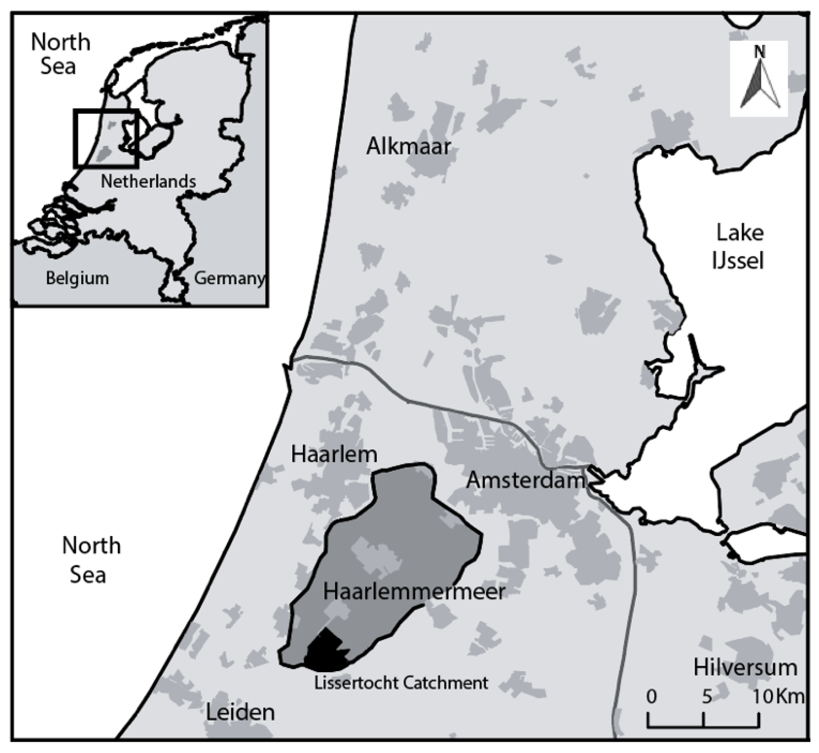
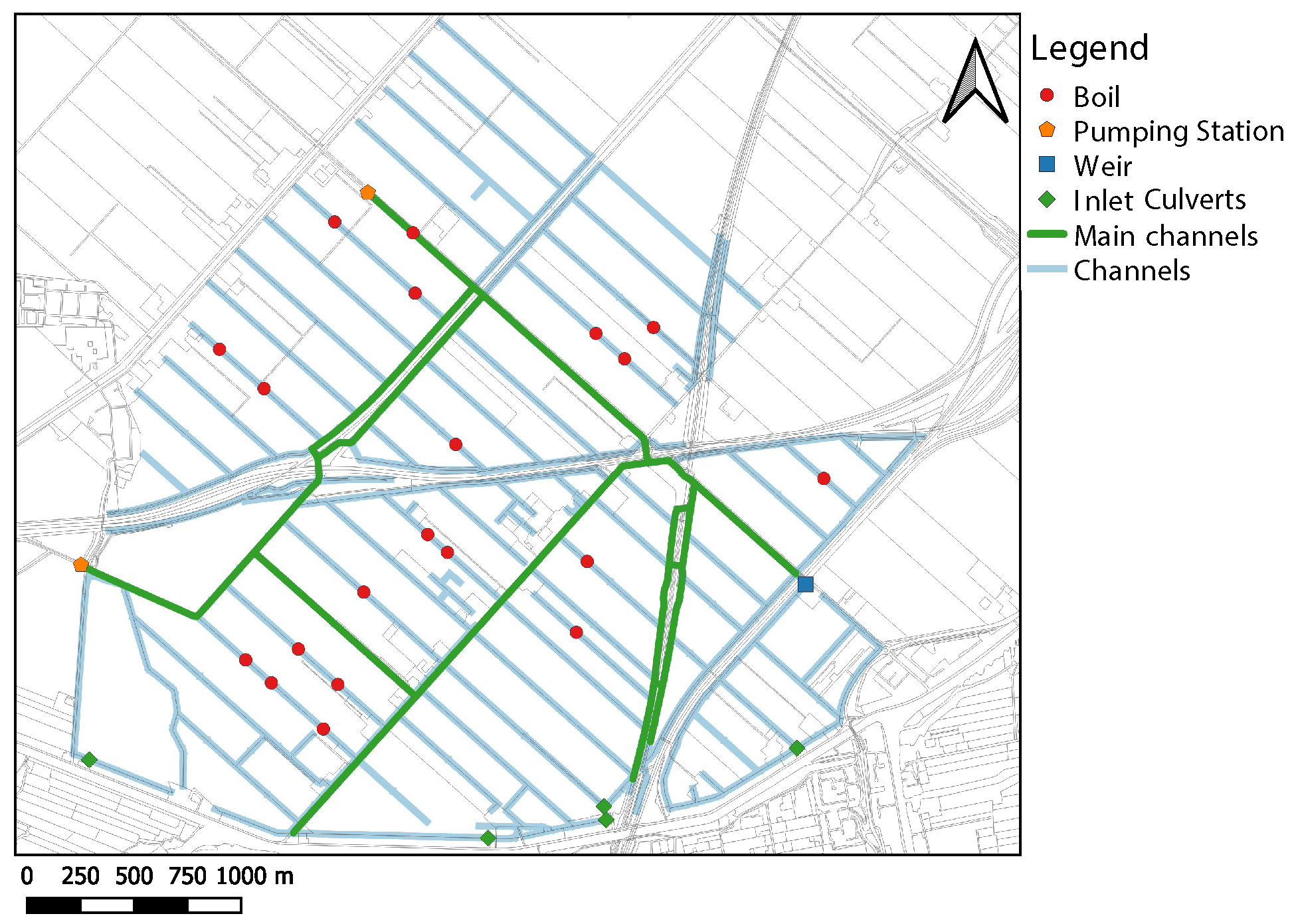
2.1. Case Study Area and Salinization Problem

The Lissertocht catchment, with a surface area of 10 km${}^2$, is a part of the former lake Haarlemmermeer (Figure 1), reclaimed in 1852, and is located approximately 25 km southwest of the city of Amsterdam. Relief in the catchment ranges between 6–3.5 m below sea level (BSL), salinity concentrations in the ditches vary between 136 and 5453 g/m${}^3$ [2]. Mean annual precipitation and mean annual potential evapotranspiration amount to 840 mm and 590 mm respectively [2]. A system of tile drains and ditches is used to quickly drain the excess precipitation. Two pumping stations with capacities 1.48 m${}^3$/s and 0.42 m${}^3$/s maintain the water level relatively constant at 6.55 m BSL (October–April) and 6.4 m BSL in summer (April–October). The latter is an auxiliary pumping station which is used only in extreme discharge events. Freshwater is diverted into the catchment through five inlets from April to October for maintaining surface water levels and improve water quality. The main land use in the study area is agriculture and the water quality and quantity requirement of the farmers varies depending on the crop cultivated.

The Lissertocht catchment is representative for deep polders in the Netherlands, where the main salinity input is deep saline groundwater exfiltration through boils (small vents directly connecting the groundwater system with surface water) [3]. Discharge of boils is low, but this is offset by their high salt concentration. Boil input (both discharge and concentration) is rather constant, as both groundwater head in the groundwater system and surface water level do not vary much. Spatial variation is large and boils are spread across ditches depending on the subsurface characteristics and surface elevation [32]. Groundwater flow directly into the ditches (diffusive seepage below the ditch itself) constitutes a second source of salts, but concentrations are lower than boils. This input is temporally more variable than boils, as it depends on the groundwater level in the adjacent field. Spatial variation of the ditch exfiltration is low. Drainage through agricultural drains (exfiltration of shallow phreatic groundwater) is the most variable input, transporting the bulk of water (and salt) during discharge events. This water is more or less fresh. In general, one ditch receives drainage water from two adjacent parcels, while the next ditch receives no drainage. Freshwater is also let into the water system of the Lissertocht catchment, through five inlet culverts, with a total capacity of approximately 0.1 m${}^3$/s (less than 10% of total pumping capacity). Ditch layout in the study area consist of ditches bordering parcels (NW-SE); these are mostly closed on one side. Perpendicular to these so-called parcel-ditches, larger ditches collect water and transport it to the two earlier-mentioned pumping stations [5]. Electrical conductivity (EC) measurements (the electrical conductivity of the ditch water is correlated to the salinity of the same water) of the surface water in the catchment have shown clear preferential pathways of water, with inlet water being mostly confined to the direct route between inlet and pumping stations. Residence times are therefore also markedly different between ditches. Residence time in transport ditches (main channels) are in the order of days, while, in parcel ditches (drainage channels) residence time can reach up to weeks or even months.

2.2. Modeling Spatial and Temporal Salinity Distributions

The surface water salinity distribution in the case study area is modeled using a 1D hydrodynamic and a salt transport model of the area. A SOBEK model is used to calculate the salt concentrations, water levels and flows in the area with a 10 min simulation time. SOBEK model calculates the flow and water levels and followed by the salt transport calculations by SOBEK 1DWAQ. In addition to this model, the input of water and salt through tile drainage and ditch exfiltration is calculated by the rapid saline groundwater exfiltration model (RSGEM) [33]. For the calibration of RSGEM, ${10}^5$ simulations were performed using different parameters and a generalized likelihood uncertainty estimation was conducted to select the parameter set used in this study following [2]. The layout of the catchment network with all structures is based on the records of the responsible water authority of the area, The Rijnland District Water Control Board. Boil locations are placed in the model in accordance with the EC routing map created in May 2011 and confirmed by additional EC routing and distributed temperature sensing (DTS) measurements conducted during this study. The layout of the Lissertocht catchment, showing the inlet culverts, pumping stations and boil locations, is shown in Figure 2. The chloride concentration of different sources of water (inlet, precipitation, boil, drain and ditch exfiltration) are used in accordance with a study conducted in Lissertocht catchment [2]. The salt transport model is calibrated using EC routing maps of the area produced in May 2011, EC measurements collected at five locations in the catchment over 2011 and 2012 and groundwater levels collected at six locations. The model is validated using the precipitation and evaporation data from the close by weather station located at Schipol airport, situated approximately 15 km northeast of the study area from 1 January 2011 until 1 January 2014 and used for calculation of the water flow and salinity in the catchment. A detailed description of the calibration of the model is given in a report for a study on smart inlets of the Lissertocht catchment [34].

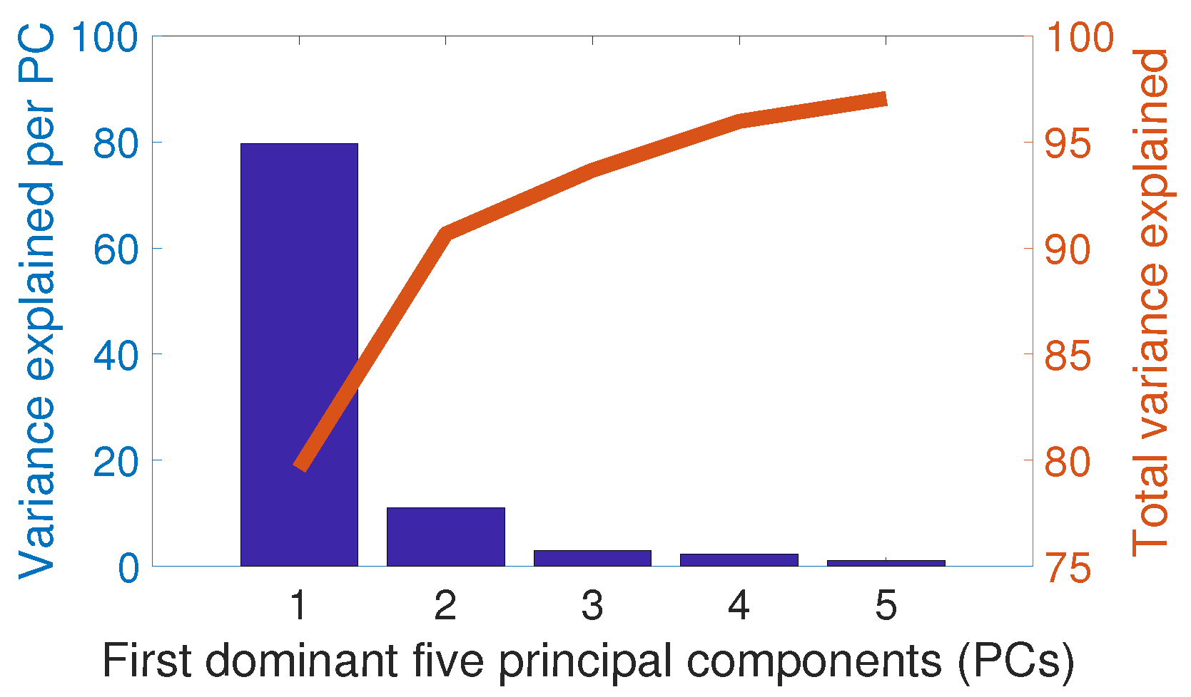
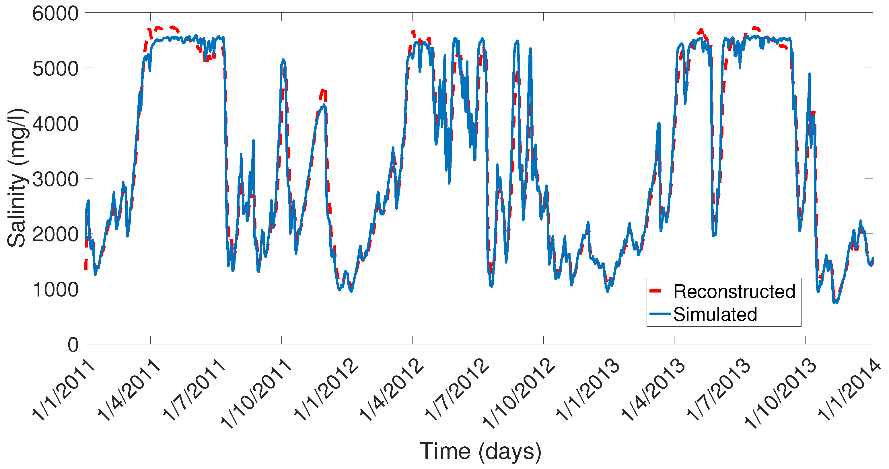
2.3. Principal Component Analysis for Estimating Salinity

Designing an optimal sensor placement requires analyzing a large-scale dynamical system of interest. Such a system is usually derived by the discretization of nonlinear partial differential equations resulting in high-dimensional discrete time models. However, the dynamics of the system can be approximated by a low-dimensional system by means of model reduction. PCA is used in this study to identify locations that capture characteristics of (annual) variations of salinity in the ditches of the catchment. Identifying the correlation between the ditches (reflecting a similar response to meteorological events, flushing water intake or proximity to boil locations) is essential for optimal estimation of the system dynamics, minimizing the number of necessary sensors by minimizing the measurement of similar, and hence redundant, system dynamics. Another important property of the PCA that is useful in sensor placement is the variance captured and represented by the PCs. Variance at a location is related to system dynamics, as it explains how much the salt concentration varies from the mean salt concentration in that location. A location with higher variance is more interesting to measure the salinity since more dynamics could potentially be captured.

We construct a low-order PCA model to reproduce the spatial salinity variation of the catchment by using the location-dependent values and time-dependent coefficients of the PCs. Considering the dynamical system of partial differential equations (i.e., Saint–Venant (SV) and advection-diffusion (AD) model, driven by boundary conditions), we restrict ourselves to states of the system describing salinity only. More information on dynamics of salt transport and control in open channels is given by Hof et al. [35].

Let $x_s\left(t\right)\in {\mathbb{R}}^n$ represent the states of the dynamical system (average daily salinity) at time t, where n is the total number of nodes in the SOBEK model. The first step of PCA is to center the measurements such that all of the measurements have zero mean; we therefore consider the variables

$$x\left(t\right)=x_s\left(t\right)-\overline{x}$$

where $\overline{x}\in {\mathbb{R}}^n$ is the mean value of the salinity levels over time; i.e., the i-th element of $\overline{x}$ represents the time mean of salinity at the i-th location/node. Simulation of the system model for N discrete time steps results in a time-snapshots dataset $X\in$ ${\mathbb{R}}^{n\times N}$ such that:

$$X:=\left[\begin{array}{c}x\left(1\right)x\left(2\right)\dots x\left(N\right)\end{array}\right]$$

It can be shown that the data X can be decomposed into an orthonormal basis (also called principal components or empirical eigenfunctions) ${\underline{\theta }}_j\in {\mathbb{R}}^n,$ $j=1,2,\dots ,n$ such that $x\left(t\right)={\sum }_{j=1}^n{\alpha }_j\left(t\right){\underline{\theta }}_j,$ $t=1,2,\dots ,n.$ That is ([36] Section 2):

$$X=\left[\begin{array}{c}x\left(1\right)x\left(2\right)\dots x\left(N\right)\end{array}\right]=\underset{{\mathsf{\Theta }}_n}{\underbrace{[{\underline{\theta }}_1\dots {\underline{\theta }}_n]}}\underset{A_{n\times N}}{\underbrace{[{\underline{\alpha }}_1\dots {\underline{\alpha }}_N]}},{\mathsf{\Theta }}_n^{\prime }{\mathsf{\Theta }}_n=I_n,$$

(1)

where ${\underline{\alpha }}_t:={[{\alpha }_1\left(t\right)\dots {\alpha }_n\left(t\right)]}^{\prime }\in {\mathbb{R}}^n$ are the coefficient vectors for time index t and can be thought of as time-dependent coefficients for reconstructing the time-snapshots via a linear combination of the time-invariant eigenvectors ${\underline{\theta }}_j$. Here $I_n$ stands for the identity matrix of size n.

In PCA, we seek a low rank approximation of the basis ${\mathsf{\Theta }}_n$ such that a low order model can approximate the dataset X in the least squares sense, i.e., we find

$$X\approx \widehat{X}=\underset{{\mathsf{\Theta }}_p\in {\mathbb{R}}^{n\times p}}{\underbrace{[{\underline{\theta }}_1\dots {\underline{\theta }}_p]}}\underset{A\in {\mathbb{R}}^{p\times N}}{\underbrace{\left[\begin{array}{ccc}{\alpha }_{1,1}& \dots & {\alpha }_{1,N}\\ ⋮& \ddots & ⋮\\ {\alpha }_{p,1}& \dots & {\alpha }_{p,N}\end{array}\right]}},p<<n$$

(2)

such that $\parallel X-\widehat{X}{\parallel }_F$ is minimized [36], where ${\parallel B\parallel }_F=\sqrt{{\displaystyle \sum _{i=1}}{\displaystyle \sum _{j=1}}{B}_{ij}^2}$ and salinity at ith location can be estimated by

$$x\left(t\right)\approx \sum _{j=1}^p{\alpha }_{j,t}\ast {\underline{\theta }}_j,t=1,2,\dots ,N.$$

(3)

In this standard PCA approach, we may desire to replace this least squares minimization of the reconstruction error by a weighted least squares where errors at some locations are penalized more than others. Weighted PCA and dealing with the presence of measurement errors is explained by Udell et al. [36].

Although the matrix factorization of X in (1) is not unique, one approach of generating and approximating it as in (2) is to employ the Singular Value Decomposition (SVD). Let the centered dataset X have the SVD given by $X=U\mathsf{\Sigma }{V}^T$, where $U\in {\mathbb{R}}^{n\times r}$ and $V\in {\mathbb{R}}^{N\times r}$ have orthonormal columns, $\mathsf{\Sigma }=\mathrm{diag}({\sigma }_1,\dots ,{\sigma }_r)\in {\mathbb{R}}^{r\times r}$, with $\sigma \ge \dots {\sigma }_r>0$, $r=\mathtt{rank}\left(X\right)$ [36]. In our example, the number of snapshots is greater than the number of states considered (i.e., $N>n$) and therefore $r\le n$. It can be shown that there is no better rank $p<r$ approximation for X in (2) than the truncation of the SVD; the first p columns of U are the eigenvectors (i.e., ${\mathsf{\Theta }}_p:=U(:,1:p)$ and the first p rows of $\mathsf{\Sigma }{V}^{\prime }$ span $A.$

Assuming that the singular values of in $\mathsf{\Sigma }$ decay rapidly, the principal components of the dataset ${\theta }_i,i=1,\dots ,p,p<<r$, will capture all the significant features of the dataset and possibly the system dynamics. The number of PCs, p, is selected such that the the total variance explained by the selected PCs exceed a user defined threshold (for example, we used 90% in this study). Each PC is a column vector with n elements and the ith row of the PCs are linearly combined through the time-dependent coefficients ${\underline{\alpha }}_t$ to reconstruct the salinity for the ith location. That is

$$x\left(t\right)\approx \widehat{x}\left(t\right)=[{\underline{\theta }}_1\dots {\underline{\theta }}_p]\underline{\alpha }\left(t\right),\underline{\alpha }\left(t\right)\in {\mathbb{R}}^p.$$

(4)

2.4. Sensor Placement Using a Greedy Algorithm

After constructing the low-order PCA model, we then aim to use this low-order model to reconstruct the spatial variation of salinity in the catchment using a limited number of measurements ($\mathit{m}\ll \mathit{n}$) available. The procedure of reconstructing the salinity state (reconstructed) vector, $\widehat{x}$ ∈ ${\mathbb{R}}^n$, in all discretization points of the catchment using m measurements taken at time step t is below.

If we assume the salinity measurements are $y\left(t\right)=C{x}_s\left(t\right), C\in {\mathbb{R}}^{m\times n},$ then we have

$$\begin{array}{cc}\hfill y\left(t\right)& \approx C{\widehat{x}}_s\left(t\right),\hfill \end{array}$$

(5)

$$\begin{array}{cc}\hfill y\left(t\right)& \approx C[{\underline{\theta }}_1\dots {\underline{\theta }}_p]\underline{\alpha }\left(t\right)+C\overline{x}.\hfill \end{array}$$

(6)

Therefore, in the absence of measurement errors, we can estimate the states ${\widehat{x}}_s\left(t\right)$ by first estimating the time-dependent coefficients $\underline{\alpha }\left(t\right)$. If the number of measurements is the same as the number of principal components in our PCA model, i.e., $m=p,$ then we simply have $\underline{\alpha }\left(t\right)={\left(C[{\underline{\theta }}_1\dots {\underline{\theta }}_p]\right)}^{-1}(y\left(t\right)-C\overline{x})$. However, if the number of measurements is greater than the number of principal components in the model, we will have an over-determined least squares problem, where we estimate $\underline{\alpha }\left(t\right)$ by solving a linear least-squares optimization problem. Once the time-dependent coefficients, $\underline{\alpha }\left(t\right)$, for the current time step t are calculated, using the PCs, salinity at all locations can be reconstructed using (4).

We then use this estimation model to find the optimal set of sensors required to reconstruct salinity in the catchment. In this present study, we have formulated the objective of the sensor placement as finding the set of node indices $J\in {\mathbb{N}}^m,J\subset \{1,2,\dots ,n\}$ for sensor locations so that the salinity state estimation (reconstruction) through (6) is optimal in the sense that it has the minimum RMSE (Equation (7)) in the main channels (See Figure 2 for the main channels). We implemented this restriction (focusing on main channels instead of all channels) by considering the water availability in the channels for irrigation. The drainage channels are very shallow and are used for draining and then transferring mainly the excess rainwater to the main channels. On the other hand the main channels have deeper water levels and connection to the freshwater inlets of the catchment which will allow the farmers to get water for irrigating their lands. Using the locations indexed in J, measurements, $y\left(t\right)$, will be collected and used to reconstruct the salinity at the main channels. The objective function that is used to evaluate the performance of the selection is given by:

$$\underset{J}{min}RMSE=\sqrt{\sum _{j=1}\frac{{\sum }_t{(x_s(j,t)-{\widehat{x}}_s(j,t))}^2}{n}}$$

(7)

where $x_s(j,t)$ is the observed or simulated salinity states at location j and time t, ${\widehat{x}}_s(j,t)$ is the reconstructed/estimated salinity state and n is the total number of nodes that salinity is estimated. RMSE is always non-negative and smaller values indicate a better accuracy of the predictions.

In this study, we employed a GA to evaluate the selection of m sensor locations. The algorithm is greedy in the sense that it sequentially places the sensors one by one. In the first step, a single sensor (location) that gives the maximum gain to the objective function is selected out of all the possible n locations. In the following step, having fixed the previous selection, the next sensor location is determined (from the remaining $n-1$ locations) that gives the largest improvement to the objective function [28]. This procedure continues until the last sensor location is determined. Algorithm 1 summarizes the pseudo code tailored for placing salinity sensors in the catchment with a greedy algorithm. Determining the (globally) optimal m locations requires finding solution to a computationally challenging combinatorial optimization problem, using an exhaustive search with m possible combinations of n possible sensor locations. As an example, placing $m=3$ sensors for Lissertocht catchment (with $n=755$ nodes) results in 2262 iterations with a GA (lines 7–12 of Algorithm 1) while the exhaustive search requires 71,443,385 iterations, where each such calculation involves estimating the coefficients $\underline{\alpha }\left(t\right)$ from measurements $y\left(t\right)$ for all $t=1,\dots ,N$, estimating the corresponding states using (4) and then computing the objective function (7) (line 11 of Algorithm 1). The combination with the best f is the global optimum for the exhaustive search. The difference in computation time and the efficiency of using a GA compared to exhaustive search is illustrated in Section 3.4.

Algorithm 1: Pseudo code of sensor placement.

3. Results and Discussions

3.1. Reference Scenario

The reference scenario was generated by simulating the Lissertocht catchment using the SOBEK model of the area from 1 January 2011 to 1 January 2014. During the simulation, a fixed flushing strategy was applied (freshwater is introduced to the system from the intakes at their maximum capacity starting from 1 April until 1 October) and the pump was operated according to the water level measurement near the pumping station following assigned water level thresholds. Figure 3 illustrates the spatial variation of salinity in the Lissertocht catchment for a snapshot taken from the reference scenario in a dry period using the SOBEK model.

The reference scenario was used to identify system behaviour and the effect of flushing on the system (the pathway of flushing water and the ditches that have no or limited access to the flushing water) using the layout given in Figure 2. Interpretation of the results revealed that the salinity in the catchment increased during the summer period despite the flushing. The main reason for this was the lack of drained precipitation that flushes the whole system naturally. Especially the small stagnant drainage ditches with boils get no or very limited amount of fresh flushing water and thus the salinity in those ditches can increase up to 5500 mg/L during summer. The high saline water from these stagnant ditches eventually flowed to the pumping station, resulting in increased salinity concentration also in the main ditches.

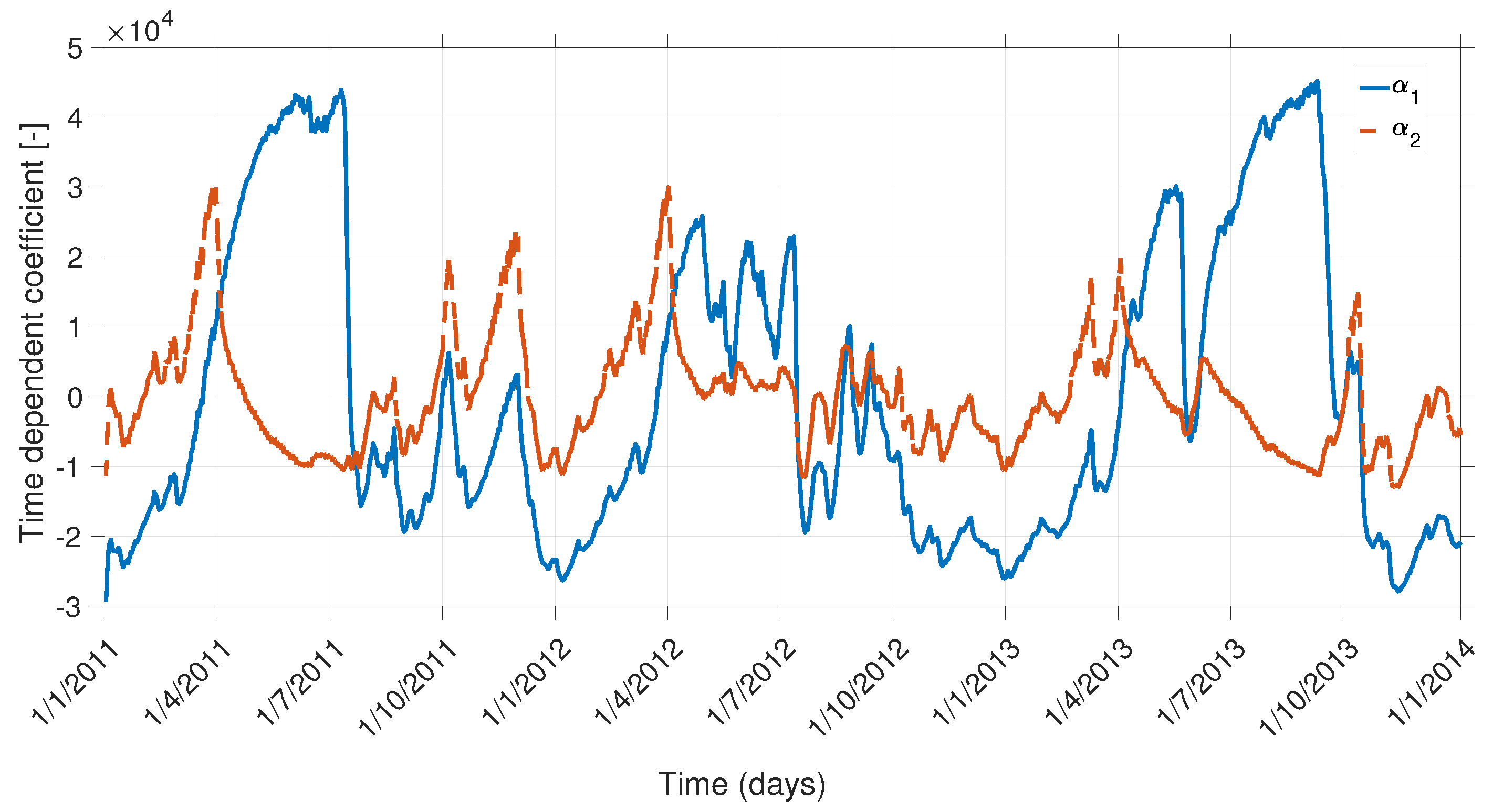
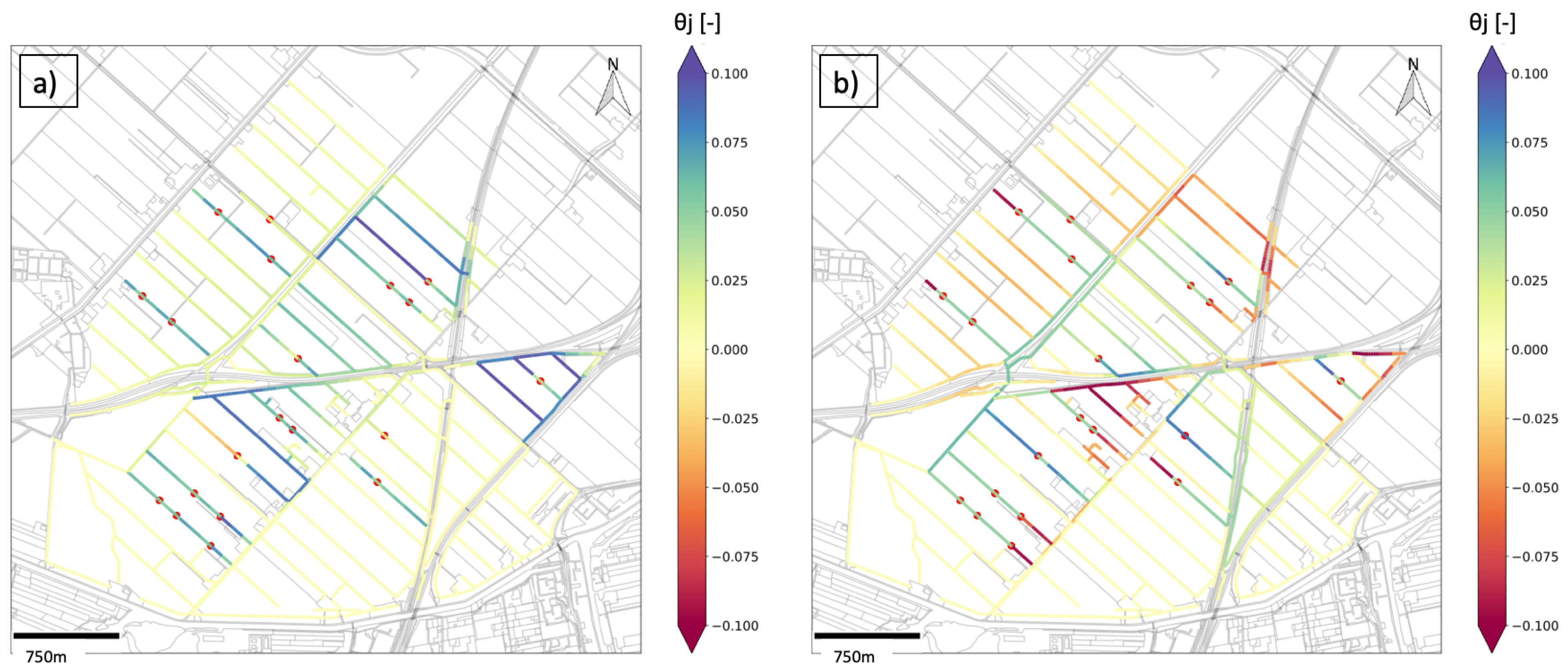
3.2. Principal Component Analysis

The SOBEK model consists of n = 755 nodes where the average daily salinity is calculated for the whole simulation period (N = 1097 days). This simulation resulted in a salinity dataset of dimension 755 by 1097. As in Equation (1), this multidimensional data set can be decomposed into 755 PCs. The percentage of variance explained by the first five PCs is shown in Figure 4. The first three PCs of this dataset explains more than 93 percent of the variance in the data (Figure 4). Figure 5 also illustrates the quality of the reconstructed salinity level over time at node 172; this is an example of reconstruction using three PCs via Equation (4).

Interpretation of the coefficients and the principal components (shown in Figure 6 and Figure 7, respectively), and the simulations were used to identify the hydrological behaviour of the catchment. As can be seen in Figure 6, the time-dependent coefficient signal of the first component started to increase in winter (wet period) and reached its peak during the summer (dry period) of each year. This behaviour was in accordance with the drainage channels with high salinity problem (due a boil or a nearby boil in the channel). This can also be seen in Figure 7a showing the PC location-dependent values of the first PC was high in drainage channels with a boil. These channels are naturally flushed when it rains (mostly in the wet period) and the salinity increased during the summer period. The time-dependent coefficient signal of the second PC decreased immediately after the 1st of April, just after the flushing of the catchment began (Figure 6). Moreover, as can be seen in Figure 7b the PC location-dependent values of the second PC were high in channels that were sensitive to flushing (main channels connecting the freshwater intakes to the rest of the catchment and drainage channels with access to flushing water). This shows that PCA can be helpful in understanding system behaviour, as was also shown by [8,9] in other applications.

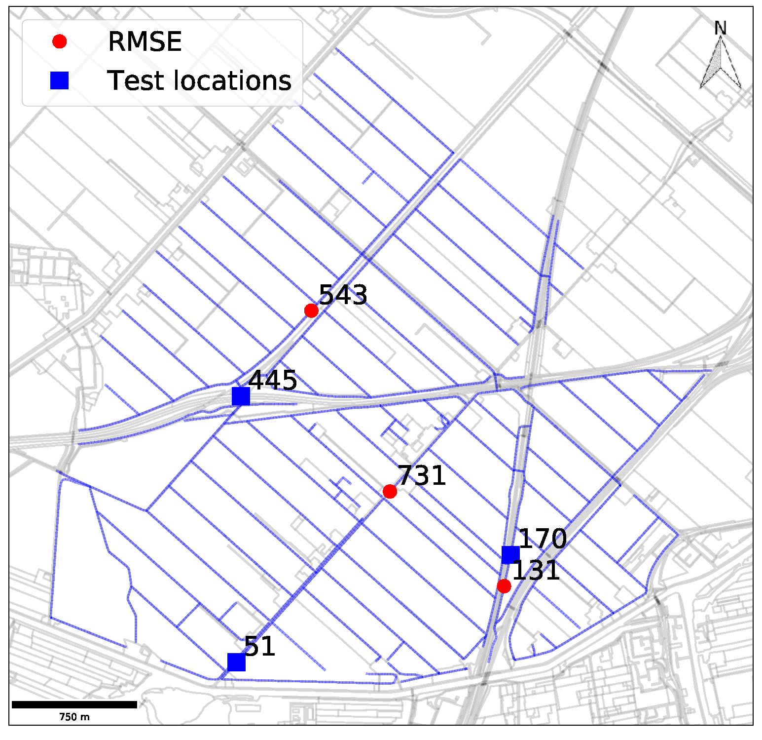
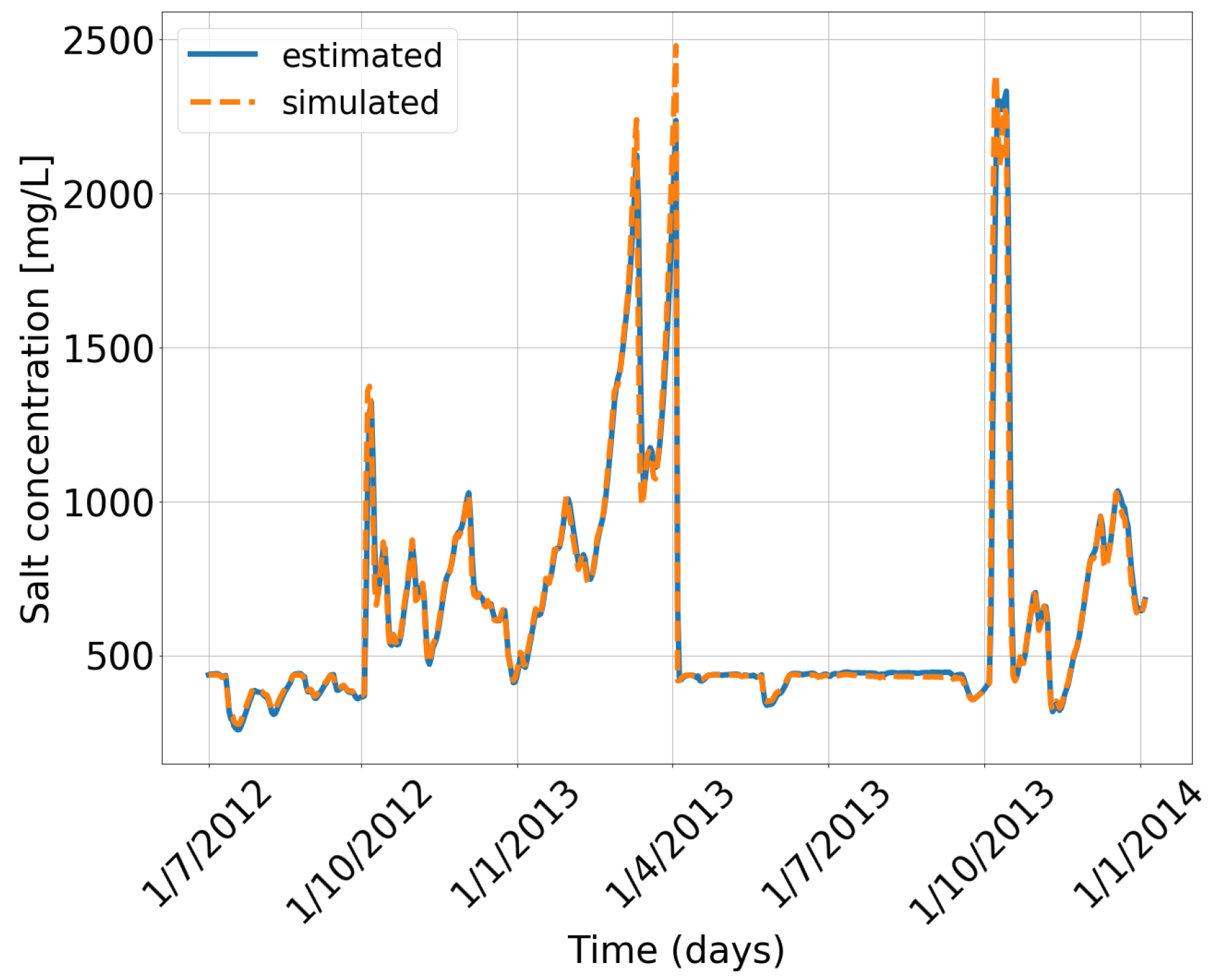
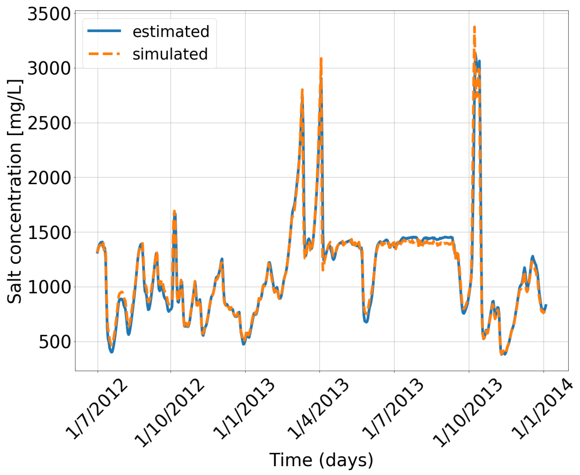
3.3. Optimum Sensor Placement Based on the Low-Order PCA Model

The low-order PCA model described in Equation (4) was based on the first three PCs of the original salinity dataset ordered according to the variance each PC explains (i.e., see the SVD in Section 2.3 with ordered eigenvalues forming the variance of each PC). We selected the first three PCs for the low-order PCA model since the variance explained by the first three PCs exceeds the threshold of 90% that we defined for this study. This property of the low-order PCA model is important in sensor placement selection using a GA. The first three PCs, capturing 93% of the variance, are used for the low-order PCA model. Selection of a new sensor locations in the GA can be conducted such that the variance covered is increased while the covariance between the selected locations are decreased by GA to place three sensors. To test the performance of sensor placements, we split the salinity dataset into two sets on time. PCA of the first part of the dataset was used to select the most dominant PCs and their corresponding location-dependent coefficients. The second part was used to test different sensor placement layouts.

Table 1. Effective sensor placements for 3 sensors by minimizing RMSE.

Node Number(s)	RMSE (mg/L)
543	140.02
543, 131	84.31
543, 131, 731	82.18

show the performance of the placement considering the objective function given in Equation (7) with a GA.

The overall performance of the placements increased with the number of sensors placed (Table 1). To illustrate the performance of the sensor placement for salinity reconstruction of three different nodes on the main channels (blue squares in Figure 8), Figure 9, Figure 10 and Figure 11 are provided. The estimation of the placement at location 51 had small mismatches compared to the simulated values with errors less than 30 mg/L. This location was close to the inlets of the catchment where the water was fresh and the salinity variance was low compared to the rest of the catchment. Therefore, the principal component values of the first two PCs was low at this location (Figure 7). The estimation of salinity was better at locations which were identified by the PCs used for the low-order PCA model like locations 170 and 445. For locations 170 (Figure 10) and 445 (Figure 11) estimations of sensor placement is very close to the simulated values. The salinity dynamics were represented accurately capturing the peaks as well as the lower salinity values observed at that location during the simulation period. Optimum sensor locations were selected such that the objective function given in (7) was satisfied over the main channels. However, if there exists a specific location of interest, the objective function can be modified for maximizing the salinity estimation performance at that location instead of evaluating the objective over the main channels.

3.4. Optimality of Placements Using Greedy Algorithm

To illustrate the solution obtained by the greedy algorithm is near optimal, we repeated the optimization using an exhaustive search by simplifying the search space used in the optimization. Every consecutive 5th node in the catchment is represented by one node and the search space was decreased to n = 151 nodes. With this reduction in the search space, the total number of possible combinations to place three sensors decreased from 71,443,385 (three combinations of 755) to 562,475 (three combination of 151). All combinations of the reduced search space were evaluated and the best was selected with the exhaustive search. For a fair comparison, we repeated the optimization using GA for the reduced space too and evaluated the performance of the selection in the full system. The locations obtained and the corresponding performances (See legend of Figure 12) by using the exhaustive search and GA are shown in Figure 12.

As expected, better performing locations are obtained by using an exhaustive search than the greedy algorithm. However, the difference in the objective values of the locations are very close. As can be seen in Figure 12 same locations are selected for the two sensors (nodes 731 and 171) and only the last sensor locations are different for GA versus the exhaustive search. The slight improvement in the objective for exhaustive search is achieved in exchange for a big difference in computation time. Finding the optimum lasted more than three days for the exhaustive search while it took only a few minutes for the GA. All the computations were performed within Python Spyder 3.3.2 for macOS High Sierra (v 10.13.6) installed on a 2.9 GHz Intel Core i5. In a larger network with larger search space and many more sensors to be placed, the application of an exhaustive search was not feasible due to the combinatorial computational burden, while a near optimal solution can easily be achieved within a limited time using our greedy heuristic.

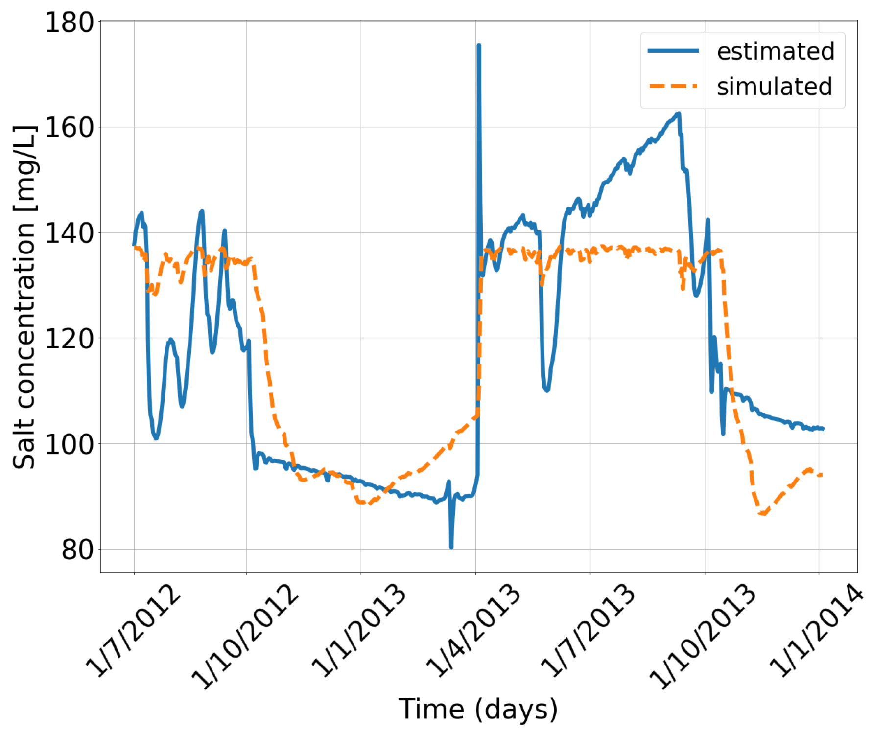
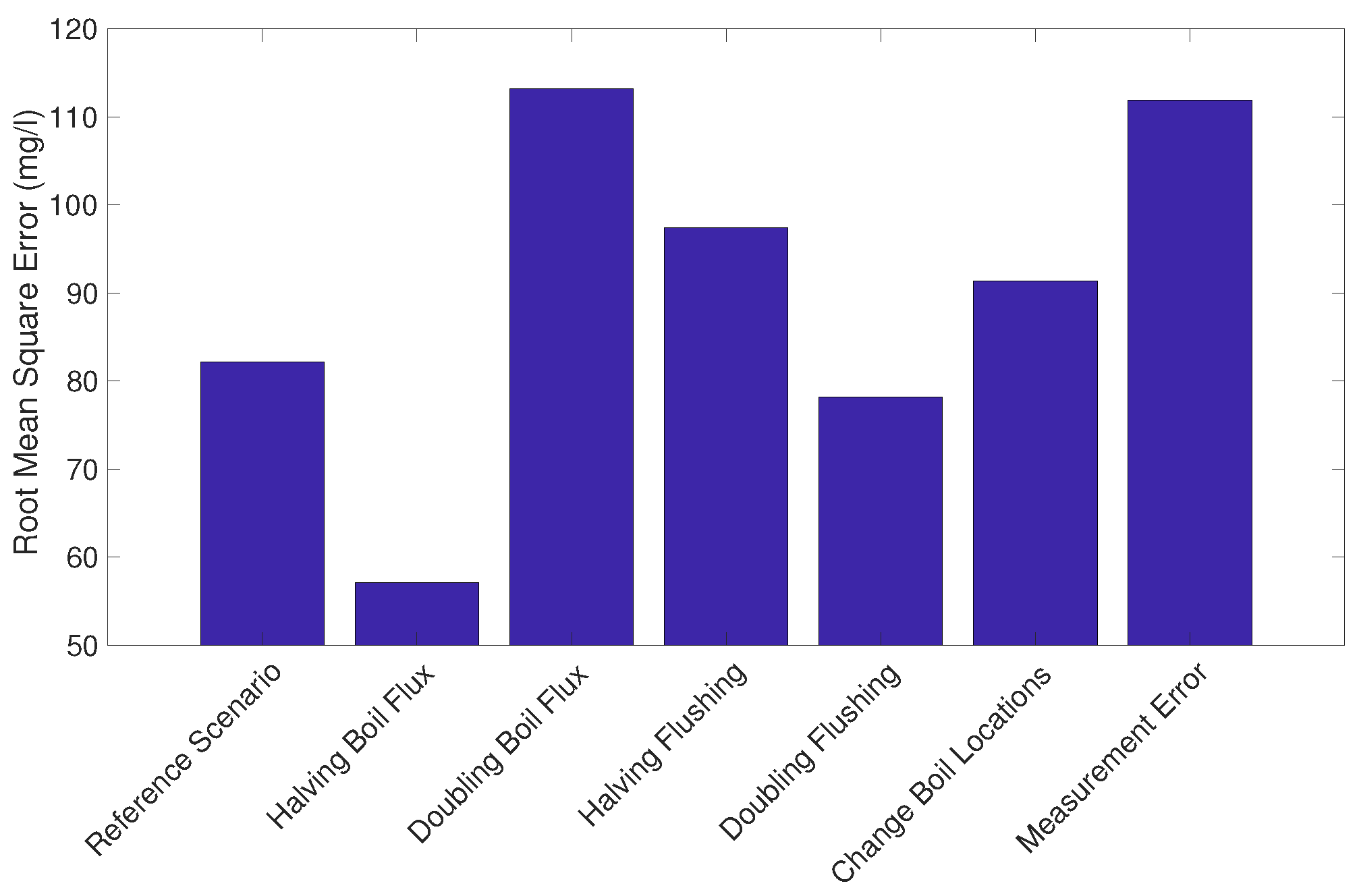
3.5. A Posteriori Assessment of Robustness of Sensor Placement to Measurement and Modeling Errors

The SOBEK model used in this study was calibrated for the reference scenario. This model was used to create the salinity dataset of the reference scenario which was then used for the sensor placement given in Section 3.3 without any consideration of uncertainties related to measurements or model errors. Therefore, to investigate the effect of possible measurement and model errors on the performance of the sensor placements, a robustness analysis is conducted in this section. Firstly, for the assessment of robustness to measurement errors, we added a random Gaussian error to the measurements used in Equation (6) with a zero mean and a standard deviation of 10. The estimated coefficients, $\underline{\alpha }\left(t\right)$, are computed using measurements with errors. We created a total of 100 measurement datasets and calculated the performance sensor placement using measurements from these datasets with errors. A decline in the performance was observed since the original placement was obtained assuming full system knowledge and without any uncertainties. RMSE increased from 82.18 mg/L to 111.86 mg/L with a standard deviation of 1.92 mg/L. In reality, it was possible that the measurement errors could be identified and filtered out which will reduce the performance reduction demonstrated here.

Secondly, the effect of possible modeling errors related to boil flux, flushing discharge and boil locations were investigated using a total of five scenarios. We started with simulating the SOBEK model by changing boil flux (halving or doubling of the reference scenario), flushing discharge (halving or doubling of the reference scenario) and boil locations (change locations of four boils). The results of these scenarios were used to create new salinity datasets for the robustness analysis with different dynamics than the reference scenario. Later, the performance of the optimum sensor placement was tested for reconstructing the salinity for these scenarios. Changing boil flux affects the total salt load entering the catchment directly. A higher and a lower mean salinity in the catchment was observed due to increased and decreased boil flux, respectively. Similarly, mean salinity in the catchment decreased in case of doubling the flushing while it increased due to half flushing. These changes affected the variance and the salinity dynamics in the catchment and resulted in changes in the performance of placements. The performance with respect to the scenarios representing possible model mismatches including the reference scenario and the mean performance of the measurement error analysis are given in Figure 13.

For all the scenarios, sensor placement performed well with small fluctuations in RMSE. The mean of the RMSE for all the scenarios was 87.57 mg/L with a standard deviation of 17.34 mg/L, indicating that the placement was robust to measurement errors and some model uncertainties. An expected performance drop for the scenarios with changing boil locations and measurement error was observed compared to the reference scenario because of the change of variance (due to changed boil locations) and uncertainty added to the measurements. This was in accordance with the results of PCA. The first PC (with the biggest variance) was attributed to the drainage channels with high salinity problems due to a boil. Depending on the presence of a boil in or a nearby drainage channel, the salinity dynamics in that channel varied considerably which effects the variance of salinity at that location. Physically, a sensor placed upstream of a boil will not capture the high salt load and will miss variance information for capturing the dynamics caused by the boil. Low-order PCA model relies on maximizing the variance captured (dynamics), therefore, lower performances were observed for scenarios changing the distribution of variance over the catchment in comparison to the reference scenario. Higher and lower RMSE values calculated for the rest of the scenarios are related to the mean salinity in the catchment. Changing the boil flux affects the total salt load entering the catchment resulting in a higher RMSE in case of doubling boil flux and a lower RMSE in case of halving the boil flux. Similar effects are observed due to the changes in flushing, resulting in a lower RMSE due to increased freshwater intake (doubling flushing) and a higher RMSE due to decreased freshwater intake (halving flushing).

4. Conclusions and Outlook

In this paper, we investigated an optimal placement of salinity sensors to represent the salinity in the main channels of a typical low-lying polder in the Netherlands. Using the salinity dataset obtained by a hydrodynamic and a salt transport model of the Lissertocht catchment, a principal component analysis was performed. PCA results showed that more than 93% of the variance of the dataset can be represented with a system of three principal components and can be used to describe the essential salinity dynamics in the catchment by means of a low-order PCA model. The accuracy of the low-order PCA model increases with the number of PCs used, and this number depends on the user defined threshold for the variance explained by the selected PCs (90% in this study). Using the low-order PCA model, optimum sensor placement of three sensors is achieved using RMSE of the estimated salinity levels as the “goodness of fit” measure. The performance of the sensor placement for salinity reconstruction is evaluated against the detailed hydrodynamic and salt transport model and is shown to yield good results with a RMSE of 82.2 mg/L.

A posteriori assessment showed that the sensor placement is robust to measurement and model errors. Increased uncertainty due to modelling and measurement errors resulted in small deviations of the performance of the placement. The placement succeeded in reconstructing the salinity of the main channels for different scenarios and are robust. Capturing the variance and related dynamics in the catchment is very important for the placements done using the low-order PCA model. Therefore, most significant performance drop of the placement is observed in case of changing boil locations. Wrong estimation of boil locations results in lack of important variance information which is crucial for capturing the dynamics caused by the boils resulting in worse salinity estimation performance for the sensor placement. This is an important outcome illustrating the importance of the hydrodynamic and salt transport model used for simulations and creating salinity datasets and of correctly locating boil sites. A good model is a must for the methodology described in this study. Extra caution and efficient ways of detecting boils is necessary for future applications.

The optimum sensor placement formulated in this study will be used in combination of a model predictive control (MPC) scheme in a follow-up research and applied to the Lissertocht catchment. Salinity and water transport dynamics will be formulated with a similar strategy developed in [6]. A state estimator (for example a Kalman Filter) in accordance with the dynamical system should be implemented for better reconstruction of the salinity state of the catchment that will be used by the MPC scheme.

References

1. Delsman, J.R.; Waterloo, M.J.; Groen, M.M.; Groen, J.; Stuyfzand, P.J. Investigating summer flow paths in a Dutch agricultural field using high frequency direct measurements. J. Hydrol. 2014, 519, 3069–3085. [Google Scholar] [CrossRef]
2. Delsman, J.R.; Oude Essink, G.H.P.; Beven, K.J.; Stuyfzand, P.J. Uncertainty estimation of end-member mixing using generalized likelihood uncertainty estimation (GLUE), applied in a lowland catchment. Water Resour. Res. 2013, 49, 4792–4806. [Google Scholar] [CrossRef] [Green Version]
3. De Louw, P.; Oude Essink, G.; Stuyfzand, P.; van der Zee, S. Upward groundwater flow in boils as the dominant mechanism of salinization in deep polders, The Netherlands. J. Hydrol. 2010, 394, 494–506. [Google Scholar] [CrossRef]
4. Oude Essink, G.H.P.; Van Baaren, E.S.; De Louw, P.G.B. Effects of climate change on coastal groundwater systems: A modeling study in the Netherlands. Water Resour. Res. 2010, 46, W00F04. [Google Scholar] [CrossRef]
5. Delsman, J.R. Saline Groundwater-Surface Water Interaction in Coastal Lowlands; IOS Press, Inc.: Amsterdam, The Netherlands, 2015; pp. 1–188. [Google Scholar]
6. Aydin, B.E.; Tian, X.; Delsman, J.; Oude Essink, G.H.; Rutten, M.; Abraham, E. Optimal salinity and water level control of water courses using Model Predictive Control. Environ. Model. Softw. 2019, 112, 36–45. [Google Scholar] [CrossRef]
7. Mahjouri, N.; Kerachian, R. Revising river water quality monitoring networks using discrete entropy theory: The Jajrood River experience. Environ. Monit. Assess. 2011, 175, 291–302. [Google Scholar] [CrossRef]
8. Noori, R.; Sabahi, M.S.; Karbassi, A.R.; Baghvand, A.; Zadeh, H.T. Multivariate statistical analysis of surface water quality based on correlations and variations in the data set. Desalination 2010, 260, 129–136. [Google Scholar] [CrossRef]
9. Ouyang, Y. Evaluation of river water quality monitoring stations by principal component analysis. Water Res. 2005, 39, 2621–2635. [Google Scholar] [CrossRef]
10. Alfonso, L.; Lobbrecht, A.; Price, R. Optimization of water level monitoring network in polder systems using information theory. Water Resour. Res. 2010, 46, 595–612. [Google Scholar] [CrossRef]
11. Alfonso, L.; He, L.; Lobbrecht, A.; Price, R. Information theory applied to evaluate the discharge monitoring network of the Magdalena River. J. Hydroinform. 2013, 15, 211. [Google Scholar] [CrossRef]
12. Raso, L.; Weijs, S.V.; Werner, M. Balancing Costs and Benefits in Selecting New Information: Efficient Monitoring Using Deterministic Hydro-economic Models. Water Resour. Manag. 2018, 32, 339–357. [Google Scholar] [CrossRef]
13. Cohen, K.; Siegel, S.; McLaughlin, T. A heuristic approach to effective sensor placement for modeling of a cylinder wake. Comput. Fluids 2006, 35, 103–120. [Google Scholar] [CrossRef]
14. Yildirim, B.; Chryssostomidis, C.; Karniadakis, G.E. Efficient sensor placement for ocean measurements using low-dimensional concepts. Ocean Model. 2009, 27, 160–173. [Google Scholar] [CrossRef] [Green Version]
15. Gangopadhyay, S.; Das Gupta, A.; Nachabe, M. Evaluation of Ground Water Monitoring Network by Principal Component Analysis. Ground Water 2001, 39, 181–191. [Google Scholar] [CrossRef] [PubMed]
16. Mishra, A.K.; Coulibaly, P. Developments in hydrometric network design: A review. Rev. Geophys. 2009, 47, RG2001. [Google Scholar] [CrossRef]
17. Keum, J.; Kornelsen, K.C.; Leach, J.M.; Coulibaly, P. Entropy applications to water monitoring network design: A review. Entropy 2017, 19, 613. [Google Scholar] [CrossRef]
18. Hart, W.E.; Murray, R. Review of Sensor Placement Strategies for Contamination Warning Systems in Drinking Water Distribution Systems. J. Water Resour. Plan. Manag. 2010, 136, 611–619. [Google Scholar] [CrossRef]
19. Shannon, C.E. A Mathematical Theory of Communication. Bell Syst. Tech. J. 1948, 27, 379–423. [Google Scholar] [CrossRef] [Green Version]
20. Lee, C.; Paik, K.; Yoo, D.G.; Kim, J.H. Efficient method for optimal placing of water quality monitoring stations for an ungauged basin. J. Environ. Manag. 2014, 132, 24–31. [Google Scholar] [CrossRef]
21. Memarzadeh, M.; Mahjouri, N.; Kerachian, R. Evaluating sampling locations in river water quality monitoring networks: Application of dynamic factor analysis and discrete entropy theory. Environ. Earth Sci. 2013, 70, 2577–2585. [Google Scholar] [CrossRef]
22. Boroumand, A.; Rajaee, T. Discrete entropy theory for optimal redesigning of salinity monitoring network in San Francisco bay. Water Sci. Technol. Water Supply 2017, 17, 606–612. [Google Scholar] [CrossRef]
23. Banik, B.K.; Alfonso, L.; Torres, A.S.; Mynett, A.; Di Cristo, C.; Leopardi, A. Optimal placement of water quality monitoring stations in sewer systems: An information theory approach. Procedia Eng. 2015, 119, 1308–1317. [Google Scholar] [CrossRef]
24. Lee, J.H. Determination of optimal water quality monitoring points in sewer systems using entropy theory. Entropy 2013, 15, 3419–3434. [Google Scholar] [CrossRef]
25. Masoumi, F.; Kerachian, R. Assessment of the groundwater salinity monitoring network of the Tehran region: Application of the discrete entropy theory. Water Sci. Technol. 2008, 58, 765–771. [Google Scholar] [CrossRef]
26. Mogheir, Y.; Singh, V.P. Application of information theory to groundwater quality monitoring networks. Water Resour. Manag. 2002, 16, 37–49. [Google Scholar] [CrossRef]
27. Owlia, R.R.; Abrishamchi, A.; Tajrishy, M. Spatial-temporal assessment and redesign of groundwater quality monitoring network: A case study. Environ. Monit. Assess. 2011, 172, 263–273. [Google Scholar] [CrossRef] [PubMed]
28. Banik, B.K.; Alfonso, L.; Di Cristo, C.; Leopardi, A. Greedy algorithms for sensor location in sewer systems. Water 2017, 9, 856. [Google Scholar] [CrossRef]
29. Banik, B.K.; Alfonso, L.; Di Cristo, C.; Leopardi, A.; Mynett, A. Evaluation of Different Formulations to Optimally Locate Sensors in Sewer Systems. J. Water Resour. Plan. Manag. 2017, 143, 04017026. [Google Scholar] [CrossRef]
30. Uber, J.; Janke, R.; Murray, R.; Meyer, P. Greedy Heuristic Methods for Locating Water Quality Sensors in Distribution Systems. In Critical Transitions in Water and Environmental Resources Management; American Society of Civil Engineers: Reston, VA, USA, 2004; Volume 40737, pp. 1–9. [Google Scholar]
31. Krause, P.; Boyle, D.; Bäse, F. Comparison of different efficiency criteria for hydrological model assessment. Adv. Geosci. 2005, 5, 89–97. [Google Scholar] [CrossRef] [Green Version]
32. Hoes, O.; Luxemburg, W.; Westhof, M.C.; van de Giesen, N.; Selker, J. Identifying seepage in ditches and canals in polders in The Netherlands by Distributed Temperature Sensing. Lowl. Technol. Int. 2009, 11, 21–26. [Google Scholar]
33. Delsman, J.R.; de Louw, P.G.; de Lange, W.J.; Oude Essink, G.H. Fast calculation of groundwater exfiltration salinity in a lowland catchment using a lumped celerity/velocity approach. Environ. Model. Softw. 2017, 96, 323–334. [Google Scholar] [CrossRef]
34. Kelderman, I. Slimmer Inlaten in de Haarlemmermeerpolder. Technical Report, Deltares. 2015. Available online: https://publicwiki.deltares.nl/display/ZOETZOUT/Slimmer+doorspoelen (accessed on 24 March 2019).
35. Hof, A.; Schuurmans, W. Water quality control in open channels. Water Sci. Technol. 2000, 42, 153–159. [Google Scholar] [CrossRef]
36. Udell, M.; Horn, C.; Zadeh, R.; Boyd, S. Generalized low rank models. Found. Trends® Mach. Learn. 2016, 9, 1–118. [Google Scholar] [CrossRef]
Figure 1. Location of the case study area (Lissertocht catchment) shown in Netherlands (adopted from [5]).
Water 11 01101 g001
Figure 2. The layout of the Lissertocht catchment showing the structures, main channels and boil locations.
Water 11 01101 g002
Figure 3. The spatial variation of salinity in the Lissertocht catchment for a snapshot (daily average of 15 July 2012) taken from the reference scenario; modeled with the SOBEK model.
Water 11 01101 g003
Figure 4. Variance explained by the first five principal components (PCs). The solid line represents the total variance explained.
Water 11 01101 g004
Figure 5. Comparison of the reconstructed salinity using three PCs and the simulated salinity at node 172.
Water 11 01101 g005
Figure 6. Time-dependent coefficients, α ̲ ( t ) , of the first two PCs.
Water 11 01101 g006
Figure 7. Principal component values, θ ̲ j , corresponding to each location for (a) first (b) second principal components. The boil locations are also shown with red dots in the ditches.
Water 11 01101 g007
Figure 8. Optimum sensor locations obtained by minimization of root mean square error (RMSE) (indicated by red circles) and three test locations (blue squares) for showing the performance of the placement.
Water 11 01101 g008
Figure 9. Performance of the sensor placement at node 51.
Water 11 01101 g009
Figure 10. Performance of the sensor placement at node 170.
Water 11 01101 g010
Figure 11. Performance of the sensor placement at node 445.
Water 11 01101 g011
Figure 12. Comparison of optimization results using an exhaustive search and greedy algorithm.
Water 11 01101 g012
Figure 13. Robustness of sensor placement to model errors using RMSE as the performance index.
Water 11 01101 g013