1. Introduction
Climate change in the Mediterranean is perceived as an intensification of existing pressures, which will imply strong reductions in water availability and further increases in water demand [
1,
2]. This will lead to the intensification of water management conflicts, due to the competition for water among different social agents and the degradation of water quality through the alteration of the hydrological cycle [
3,
4]. In some regions, current water uses cannot be maintained in the future [
4]. The solution to these problems will imply profound social changes, progressive reduction of water demand, and reallocation of water availability to those uses that are deemed socially as more appropriate. Thus, guidance is needed to assess the effort and effectiveness of broad management strategies [
1].
Projections of climate studies show that the effects of climate change will ultimately affect water resources availability and thus, have an impact on water management [
1]. Hydrological stress is expected to increase in central and southern Europe. For the 2070s, the percentage of surface area under conditions of severe water stress is expected to increase from the current 19% to 35%. Populations living under water stress conditions in regions from 17 countries of western Europe are projected to increase by between 16 to 44 million. It is also predicted that the volume of certain rivers may diminish up to 80% during summer season and reservoirs lose resources due to a decrease of rainfall. A reduction of average natural water resources will produce increasingly more frequent and more intense episodes of water shortage [
2]. Alterations in the variability of water resources are also foreseen with climate change, which involves the intensification of the frequency and magnitude of extreme events, like floods and droughts, resulting into important impacts on the population [
3,
4]. Furthermore, higher temperatures are expected to increase water demand for irrigation and urban supply. Water is increasingly becoming a limiting factor for sustainable economic growth and development [
5]. Its allocation has significant impacts on overall economic efficiency, particularly with growing physical scarcity in certain regions. Greater water supply variability further increases vulnerability in affected regions. Water also has become a strategic resource involving conflicts among those who may be affected differently by various policies [
6].
Scenarios of water resources availability are developed from climate projections but need to take into account water management, infrastructures, and demands. Hydraulic infrastructure plays a critical role to make water available to users by overcoming the spatial and temporal irregularities of the natural regimes. In water-scarce regions, the impacts of climate change on natural resources will affect water uses through water resource systems, which perform functions of regulation, transportation, and distribution of water resources. In the Mediterranean region, most water resources systems are highly developed and have achieved a profound transformation of the natural characteristics of water resources to accommodate the needs of demands. Climate change impacts on the water will have a large impact on human water security and biodiversity [
7]. There are several hundred studies on the potential impacts of climate change on water resources in the Mediterranean which apply many different approaches [
8]. Although the results are diverse and sometimes contradictory, a common element is that one of the primary impacts of climate change will be a reduction of water availability in this region [
2,
9].
In order to achieve future objectives for water management under climate change, science has developed a set of tools to understand uncertainty [
10], assess future impacts [
11,
12], and facilitate policy development [
4,
13]. The challenges of water management under climate change conditions will have to be met through adaptation. Adaptation, in this study, involves the adoption of measures with a potential to reduce the impact itself or have the influence of the driver on the impact. Evaluating adaptation of the water resources sector to climate change is not an easy task, due to the broad range of objectives of water policy, from social choices for the allocation of water to technical alternatives. Society is becoming increasingly concerned about the environment as the population water needs continue to grow and climate change imposes further limitations. Furthermore, the likelihood of climate change impacts will continue to increase as long as adaptation strategies are not carried on. However, defining the adequate strategies requires multiple efforts from the understanding of impacts to the selection of alternatives that respond to local development priorities. Modeling the system at risk provides a measure of the potential need for adaptation and the benefit of the intervention. Moreover, models provide means to represent regional variations of the effect of a warming climate on soil-moisture, evaporative losses, and changes in precipitation, irrigation, water availability, and urban or tourist use. Döll [
14] offered, for the first time, a global analysis of irrigation requirements under climate change. Her results highlighted that two-thirds of the global area equipped for irrigation in 1995 would possibly suffer from increased water requirements, and on up to half of the total area (depending on the measure of variability), the negative impact of climate change was more significant than that of climate variability. Following the same methodology, Rosenzweig et al. [
15] used a suite of models to evaluate scenarios of water resources for agriculture in a changing climate in five major agricultural regions: USA, Europe, China, Brazil, and Argentina. Iglesias et al. [
13] evaluated the need for additional irrigation as an adaptation strategy considering that scenarios of urban water demand are driven by changes in population and lifestyles. The calculation of changes in irrigation requirements aims to reach demand satisfaction according to the assumptions on the technological capacity of the country and is limited by the country environmental requirements. Logar and Van den Bergh [
16] provided an overview of methods for the assessment of the costs of droughts.
The aims of the study were to estimate water availability changes due to changes in runoff and to evaluate the effect of adaptation choices on the distribution of water availability, under climate change. The analysis was carried out in representative basins in the Mediterranean region. Following this introduction,
Section 2 presents the data and methods,
Section 3 provides the results and discussion, and
Section 4 discusses the conclusions of the study.
2. Materials and Methods
2.1. Approach
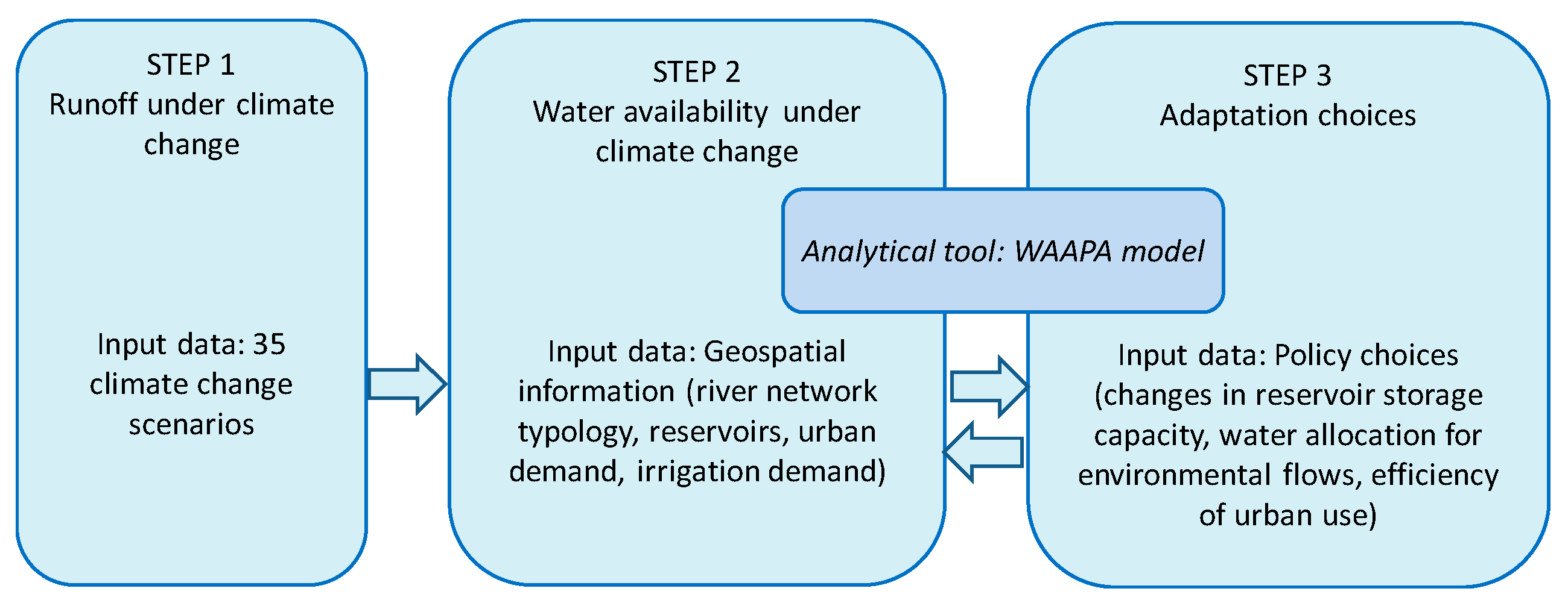
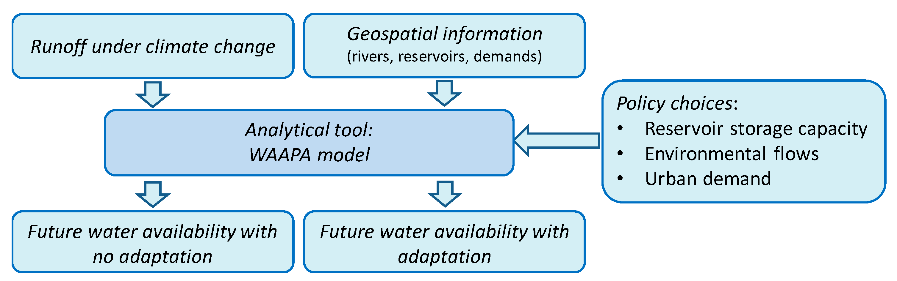
Our methodological approach is presented in
Figure 1. The analysis consisted of three steps: estimation of runoff under climate change, calculation of water availability changes due to changes in runoff, and evaluation of the adaptation choices that can modify the distribution of water availability under climate change. The adaptation choices included changes in reservoir storage, environmental flow requirements, and efficiency of urban water use. The analytical tool to estimate water availability and adaptation choices was the Water Availability and Adaptation Policy Analysis (WAAPA) model [
1,
2].
2.2. Geographic Extent: Basins under Analysis
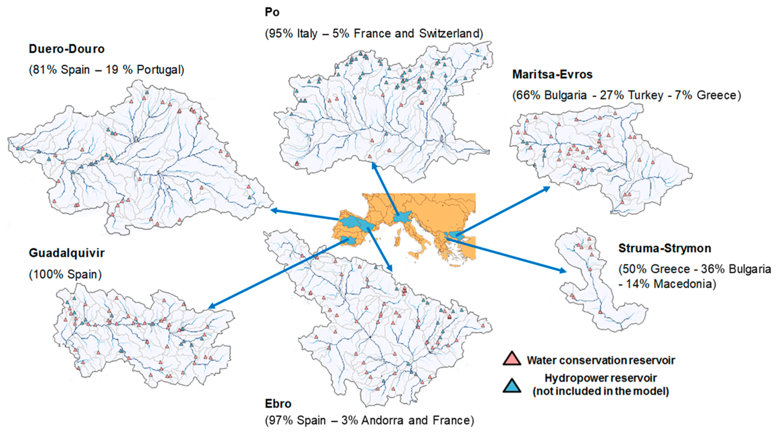
The analysis was carried out in six representative basins from southern Europe: Duero-Douro, Ebro, Guadalquivir, Po, Maritsa-Evros, and Struma-Strymon (
Figure 2). The main characteristics of these basins are presented in
Table 1. These basins cover a representative range of water management conditions in southern Europe. Most of the basins are transboundary basins. Only the Guadalquivir basin is entirely in Spain. Several fluvial regimes coexist in these large basins: nival, pluvio-nival, pluvial, ephemeral, among others. Po river basin has the largest specific runoff, with 550 mm, and Maritsa-Evros has the lowest, with 75 mm. Specific runoff in the other basins ranges from 140 mm to 190 mm.
Agriculture is the largest consumptive water use in all basins. Agriculture and the derived agroindustry account for a significant fraction of local economies. The basins also provide drinking water to 30 M inhabitants, with half of this amount located in the Po basin. Flow in the rivers is regulated by a large number of reservoirs. Most of these reservoirs are multipurpose in nature, including flood control, hydropower, irrigation, industrial, and drinking water supply. We focused our analysis on the water conservation reservoirs, and thus, reservoirs operated exclusively for hydropower were excluded from our model.
2.3. The WAAPA Model
The analyses of water availability were carried out with the Water Availability and Adaptation Policy Analysis (WAAPA) model [
1,
2]. WAAPA is a model that simulates reservoir operation in a water resources system. Basic components of WAAPA are reservoirs, streamflows, and demands. These components are linked to nodes of the river network. WAAPA allows the simulation of reservoir operation and the computation of supply to demands from an individual reservoir or from a system of reservoirs accounting for ecological flows and evaporation losses. From the monthly time series of supply volumes, supply reliability can be computed according to different criteria. Other quantities may be computed using macros that repeat the basic simulation procedure: The demand-reliability curve, the maximum allowable demand corresponding to given storage or the required storage volume to meet a given demand, all according to different reliability criteria.
WAAPA model is based on a basic joint reservoir operation model. The joint reservoir operation model simulates the behavior of a set of reservoirs that supply water for a set of prioritized demands, complying with specified ecological flows and accounting for evaporation losses. It takes as input the monthly inflows in every reservoir, the monthly required environmental flow in every reservoir, the monthly demand values sorted by priority with the corresponding return flow, the reservoir data in every reservoir (monthly maximum and minimum capacity, storage-area relationship, and monthly evaporation rates), and the reservoir’s initial condition in every reservoir (initial storage). In this study, we assumed that the required water to satisfy demands was first released from the reservoirs located at low areas of the basin. If these reservoirs were full and received more contributions, uncontrolled spills would be released and water would miss out the system. On the other hand, if upstream reservoirs were full and received more inflows, the extra water would be collected by the downstream reservoirs. In each time step, the model performed the following operations:
Computed evaporation in every reservoir and reduced available storage accordingly.
Satisfied the environmental flow requirement in every reservoir with the available inflow. Environmental flows were added to the downstream reservoirs’ inflows.
Increased storage with the remaining inflow, if any. Also, computed excess storage (storage above maximum capacity) in every reservoir.
Satisfied demands ordered by priority, if possible. Used excess storage first and then the available storage starting from higher priority reservoirs.
If excess storage remained in any reservoir, the model computed uncontrolled spills.
The result of the joint reservoir operation model was a set of time series of monthly volumes supplied to each demand, monthly storage values, and monthly values of spills, environmental flows, and evaporation losses in every reservoir. From this output, demand reliability could be computed applying any conventional procedure.
2.3.1. Topological Data
The WAAPA model of the basins under analysis was derived from the Hydro1k dataset [
19], a geographic database of global coverage that provides a number of topographically derived datasets. We used the digital elevation model and the derived datasets of flow direction, flow accumulation, and sub-basins. Reservoir data were obtained from the ICOLD World Register of Dams [
20]. This is the most comprehensive global dataset of dams and provides information on dam purpose, total reservoir capacity, and total reservoir area, among many other variables. In order to be included in the WAAPA model, these dams had to be geo-referenced. Location for some dams was available in the geo-referenced database of dams included in Aquastat and FAO’s information system on water and agriculture [
20]. The remaining dams were geo-referenced by identification on aerial imagery. Dam locations were fitted to the river network derived from the Hydro1k data set. Model topology was divided into the sub-basins included in the Hydro1k dataset plus the subbasins derived from dam locations. A post-processing step removed sub-basins of less than 10 km
2 and split sub-basins larger than 10,000 km
2. Since hydropower reservoirs are generally not managed for water conservation, we removed the reservoirs that were listed in the ICOLD database as managed exclusively for hydropower. The resulting models are shown in
Figure 2. It is noticeable that hydropower reservoirs account for more than 40% total reservoir capacity in the basins under analysis.
2.3.2. Socioeconomic Data
We estimated the demand for urban water supply from the population distribution over the basins. The population was taken from the Global Rural-Urban Mapping Project (GRUMP) dataset, provided by the Socioeconomic Data and Applications Centre of NASA [
18]. We used the population count grid, available with worldwide coverage at 30 arc-second resolution grid cells and associated with data for the year 2000. Population estimates derived from this dataset are higher than figures produced from basin authorities, but it provides also the spatial distribution within the basin. Urban demand was estimated by considering a reference per-capita consumption of 300 liters per person and day (l/pd). This reference figure is, in fact, smaller than current actual water consumption. Dividing Aquastat estimates of water withdrawal for domestic use by the current population, we obtained an average consumption of 475 l/pd for Spain, Portugal, Italy, and Greece. Therefore, the figure of 300 l/pd should be interpreted as a policy target. For future projections, we considered that the population remained constant and per-capita consumption was reduced through policy in the range 300–175 l/pd. Population projections [
21] are roughly coincident for southern European countries (Spain, Portugal, Italy, and Greece), but they differ strongly according to the Shared Socioeconomic Pathway (SSP) chosen. Two SSP projections imply strong changes (larger than 20%) but of different sign (negative for SSP3 and positive for SSP3). The remaining SSP imply mild population changes (less than 10%) with a different sign across countries. Given this diversity of projections, it was decided to simulate with a constant population in order to simplify the analysis. An estimate of current agricultural demand can also be obtained from the Global Map of Irrigation Areas (GMIA), available in Aquastat [
22,
23].
2.4. STEP 1: Runoff under Climate Change
We compiled 16 model runs for the current period and 35 climate change scenarios for the future period (
Table 2). The data sources are: PRUDENCE project (Prediction of regional scenarios and uncertainties for defining European climate change risks and effects project, [
24]) under the Special Report on Emissions Scenarios (SRES) [
25] emission scenarios A2 and B2 (projections for A1 and B1 emission scenarios were not available in PRUDENCE); the ENSEMBLES project (supported by the European Commission’s 6th Framework Programme, contract number GOCE-CT-2003-505539, [
26]) under SRES emission scenario A1B (the E1 emission scenario was not considered because it is not included in SRES); the application of the PCRGLOBWB grid-based global hydrology model (grid 5 arcminutes) [
27] to the Inter-Sectorial Impact Model Intercomparison Project (ISIMIP, [
28]) under the Representative Concentration Pathways (RCPs) RCP2.6, RCP4.5, RCP6, and RCP8.5 [
4,
28,
29,
30]. Monthly flows in sub-basins were downscaled and estimated from gridded climate projections following the method proposed by González-Zeas [
31]. Although these variables are subject to large uncertainties, they can reproduce the basic seasonal and spatial characteristics of surface hydrology and are routinely used to undertake water resources impact analyses [
1,
4]. We ranked the results obtained for runoff under different climate change scenarios and climate models to produce an ensemble of projections to describe climate and model variability.
2.5. STEP 2: Changes in Water Availability
As stated, potential water availability was estimated with the WAAPA model [
1,
2]. In this study, potential water availability was considered the maximum amount of water that can be supplied at a certain point of the river network to satisfy a defined demand, and the specified reliability requirements were taken into account. We assumed that water availability for the historical period is approximately equal to current water use. This assumption is justified because water availability in southern Europe is the result of costly infrastructure development to satisfy water needs. Water availability in future scenarios was compared to current water availability to identify potential risks of future water scarcity. We also assumed that the decrease in water availability is a proxy for the required effort of adaptation to climate change. The larger the projected decrease of water availability, the larger the effort to cope with water scarcity will be in the future. We ranked the results obtained for water availability under different climate change scenarios and climate models to produce an ensemble of projections to describe climate and model variability. Larger variations implied less confidence in our conclusions.
The methodology of analysis in the WAAPA model was based on a computation module to estimate water availability provided by a set of reservoirs in a water resources system under different hypotheses. The basic module of WAAPA was repeatedly run with varying demand values until the pre-specified reliability was met. Prior to demand satisfaction, water was allocated to supply environmental flows, estimated as the 10th percentile of the marginal distribution of monthly streamflow. System performance was evaluated as gross volume reliability. Availability was obtained under the hypothesis of 98% reliability. These characteristics corresponded to average conditions in the region and were used to obtain an estimate of potential availability with the purpose of comparison among basins and scenarios.
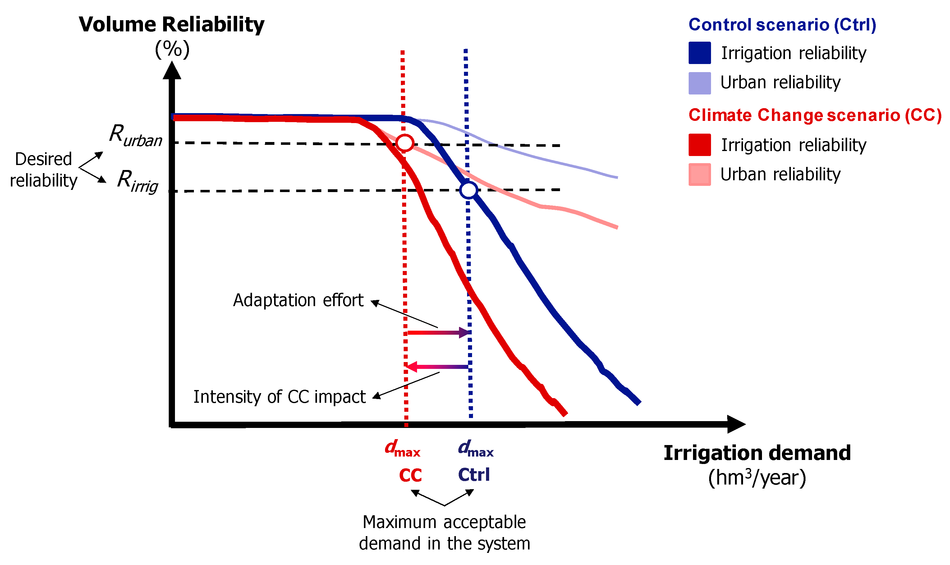
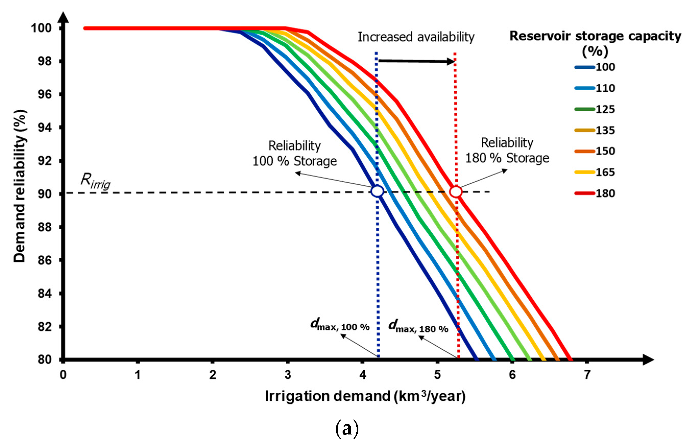
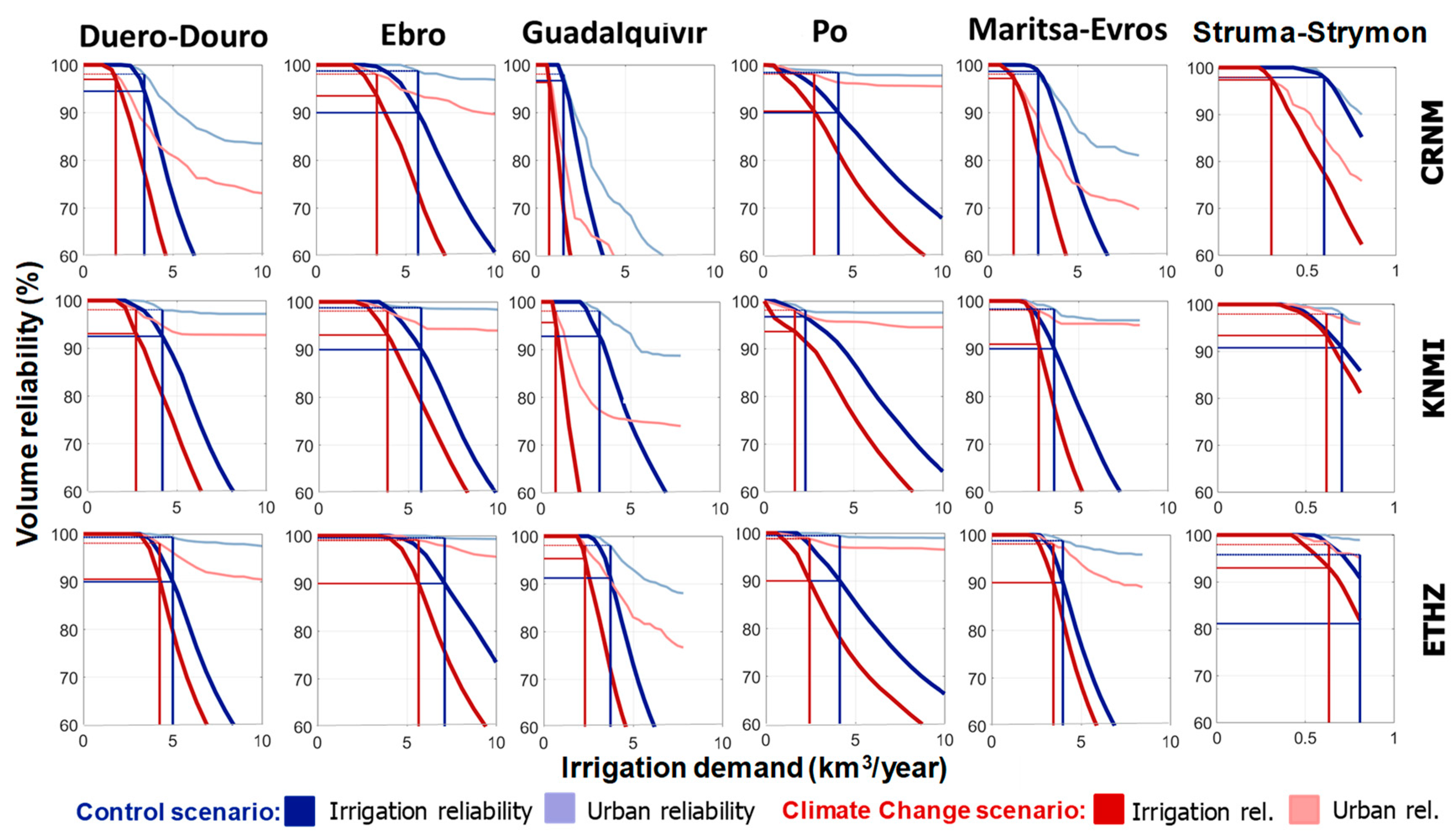
The analysis was based on the demand-reliability curve. The demand-reliability curve represents the reliability of urban and irrigation demands as irrigation demand varies. Potential water availability for irrigation was addressed, for pre-specified reliability, when the difference between two values of irrigation demand was lower than 0.1% of mean annual flow. We considered one mixed demand grouping urban and irrigation demands. We assumed a monthly distribution consisting of a combination of 20% urban demand and 80% irrigation demand. This distribution is typical in southern Europe, where irrigation accounts for roughly 80% of water consumption. The methodology of analysis is illustrated in
Figure 3, where the reliability of the urban demand is represented in a lighter color, and the reliability of irrigation demand is represented in a darker color. As shown in
Figure 3, the analysis was applied in two different periods: the control period (blue) and the climate change period (red). Water availability was determined by specifying the required reliabilities for urban and irrigation demands. We used required values of 98% (R
urban) and 90% (R
irrig.) gross volume reliabilities for urban and irrigation demands, respectively. Water availability for irrigation is the minimum demand value that satisfies both requirements simultaneously. Water availabilities for irrigation in the current and climate change scenarios are represented by vertical lines of blue and red colors. The comparison between the water availability for irrigation in control and in the climate change scenario provides a proxy variable to estimate the effort of adaptation to climate change. If the objective of water policy is to maintain adequate reliability for both urban (R
urban) and irrigation (R
irrig.) demands, we can estimate the adaptation effort from the difference between water availability for irrigation in control (d
max Ctrl) and in the climate change scenario (d
max CC). The larger the difference between current and future water availabilities for irrigation, the greater the effort required to compensate for climate change through adaptation.
2.6. STEP 3: Adaptation Choices
The analysis of adaptation choices included policy changes that affect water availability. For this in-depth analysis, we selected the three climate simulations under the A1B emission scenario (CRNM, KNMI, and ETHZ). We selected this emission scenario because it is a middle-of-the-road scenario that produces water availability projections in the upper, middle, and lower range of the ensemble in most basins analyzed. The methodology for the analysis of the adaptation measures is presented in
Figure 4. The obvious policy choice is reducing water allocation to agriculture in order to protect other uses with higher priority, such as urban supply. We named this policy as the reference policy. However, sometimes the reduction of water availability for agriculture cannot be faced only with water-saving measures, and the reduction is even more in developed countries, where the irrigation systems are technologically advanced and show high water use efficiency. Therefore, the projected decrease of water availability was addressed through a range of adaptation measures. We presented an analysis of the required intensity, range, and effectiveness of these measures. In this study, the intensity of additional management measures was the degree of implementation of a specific measure (e.g., an increase of storage of 10% or 20%), the range was the maximum effect obtained with the policy (e.g., compensate for 10% of the reduction of water allocation to agriculture), and the effectiveness was the ratio between the range and the intensity. The trade-offs between these policies and the reference policy were globally evaluated for the selected basins to determine their future water availability for agriculture.
We assumed that the policy target for future scenarios is to guarantee safe drinking water and provide adequate reliability for irrigation demand to protect the agroindustry. As mentioned, with the strong reduction of water availability obtained in the analysis for most basins, the obvious adaptation measure is to reduce water allocation to irrigation, in order to protect the reliability of urban demand, which is considered a policy priority. The estimated required reduction would be the difference between water availability in the control scenario and water availability in the future scenario, in order to restore the same level of performance that is observed in the control scenario. The impact of the reduction of water allocation to agriculture can be mitigated by maximizing water use efficiency for agricultural use. These policies are already implemented or under implementation in many irrigation districts of southern Europe, and it is expected that by the time horizon contemplated in the long term scenario, all irrigation in southern Europe will achieve high standards of water use efficiency. However, maximizing water use efficiency may not compensate for the strong reduction of water availability. In this case, the reduction of water allocation will imply the abandonment of irrigation in a fraction of the land currently under cultivation. This is a costly measure due to the economic dependence of the region on the irrigated agriculture sector [
13].
We explored the possibility of other policy alternatives that may help reach the objective of adequate supply reliability. The trade-offs between some of these policy measures and irrigation demand management were analyzed in this study. The procedure is illustrated in
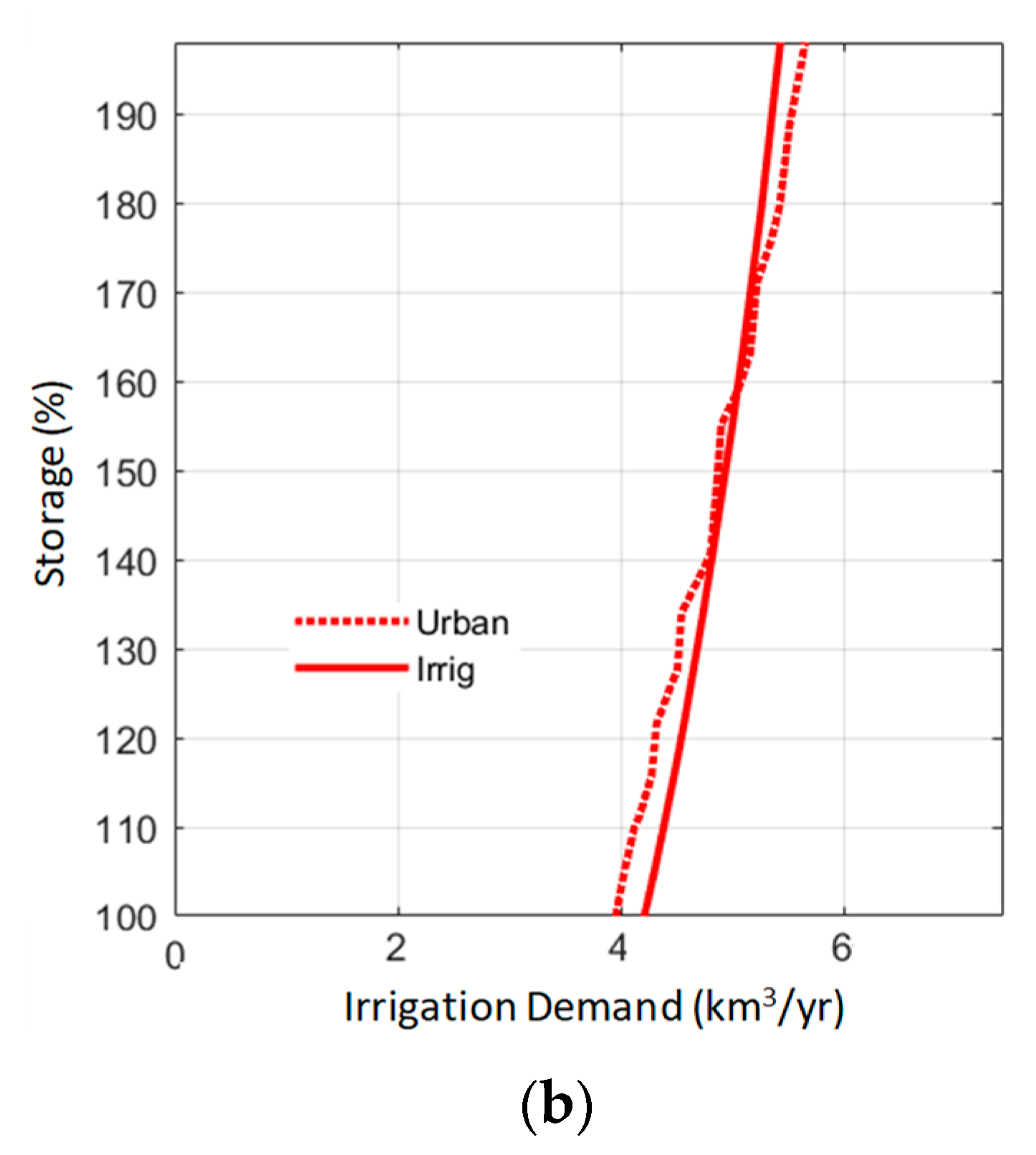
Figure 5, where, as an example, we took increased reservoir storage as the correlative policy.
Figure 5a represents the demand-reliability curve of the irrigation demand for varying values of reservoir storage capacities, expressed as a percentage of current values. Water availability was increased with the increase in the reservoir capacity. If we applied the same methodology to the demand-reliability curve of the urban demand, we could obtain the evolution of water availability determined by the reliability of urban demand.
Figure 5b represents the evolution of water availability (e.g., irrigation demand reliability = 90%, urban demand reliability = 98%) as a function of both limiting cases. The final curve would result from the application of the most limiting case. This curve would determine the potential to partially avoid the required reduction of water allocation to irrigation if the policy of increasing storage capacity is implemented.
We analyzed the following correlative policy measures: (1) increase in reservoir storage, (2) modification of water allocation to environmental flows, and (3) increase in the water use efficiency of urban supply. Reservoir storage was the dominant management measure during the 20th century [
1,
32]. During that period, reservoir storage was dramatically increased in order to provide adequate supply for the emerging water uses that were developing. Although the activity in dam construction has experienced a significant reduction in southern Europe, some studies suggest that increased reservoir storage is an adequate response to the increased hydrologic variability projected by climate models [
33,
34]. We tested this hypothesis. We represented the increased reservoir storage in the WAAPA model by increasing the capacity of existing reservoirs. We chose this option as a conservative estimate since the additional storage would produce better results if its location was optimized. However, there is no clear guidance on where the future reservoirs might be located in the basins under analysis, and environmental, social, and technical constraints favor a heightening of existing dams over building reservoirs in new sites. Water allocation to environmental flows may be the most relevant water management policy in the current century. The paradigm shift induced by the implementation of the Water Framework Directive has reduced the emphasis on demand satisfaction and has focused the attention on the ecological status of water bodies. The need for establishing environmental flow constraints to water abstractions is now widely recognized, but there is a clear trade-off between the amount of available water that is allocated to natural ecosystems and to human uses. There is a wide array of methods to determine minimum environmental flow, and its practical application is far from systematic and unified. The environmental policy may establish more restrictive or more flexible conditions to balance the impacts of human activities on the environment and on regional economies. We explored this trade-off by changing the reference values for environmental flows allocation. We applied a simple hydrologic method to establish minimum environmental flows based on the percentile of the marginal distribution of monthly flows. This method was taken from Spanish legislation [
6], which currently establishes a range between 5% and 15% percentile, with the central value of 10% as the suggested reference. In our analysis, we covered the range from 0% to 20% percentile, which implies both increases and decreases in water availability with respect to the reference condition. The third adaptation policy under consideration was to improve the efficiency of urban use. This is a natural consequence of a scenario of increasing water scarcity, where all uses should maximize efficiency. The different reliabilities of urban and irrigation demands mean that one unit of water released from urban allocation could imply an increase in larger than one unit of water availability for the competing use. This option was explored by reducing the per-capita water consumption from 300 l/pd to 175 l/pd, which is the figure currently achieved in the most efficient cities in southern Europe.
Each of these factors was analyzed in combination with a reduction of water allocation to irrigation by computing the reliability for the urban supply and the irrigation demands that result from the joint application of both measures. If the reduction of water allocation to agriculture was applied in combination with another policy, the resulting reliability values for every demand present in the system could be plotted against both adaptation efforts. The line that corresponds to the minimum required reliability for every demand type enabled us to identify the required efforts when both measures were applied in combination (
Figure 5).
2.7. Limitations of the Methodology
Some limitations of the methodology should be noted. First, the potential water availability is a theoretical upper limit by assuming that any demand at a given point in the stream network can be supplied from any reservoir located upstream from it. Real systems are usually managed by taking into account more conditions and constraints. They are either managed individually to supply local demands or grouped in independently managed systems. WAAPA results should only be considered as an upper bound of the water availability that could be obtained in practice. Second, in one case, the model was run with one mixed demand grouping both types, urban and irrigation, assuming a distribution of 20% urban and 80% irrigation. Third, system performance was evaluated as gross volume reliability. Fourth, the analysis of policy option to manage water availability for agriculture was performed in one representative emission scenario (SRES emission scenario A1B) with three climate change scenarios (for the RCMs CRNM, KNMI, and ETHZ). Fifth, the proposed policy measures were applied sequentially and not by combining fractions of each one simultaneously. Sixth, we assumed that the reservoir capacity of the basin would be equal or higher than the current reservoir capacity. Finally, the effectiveness of the policy measures was estimated regardless of the cost of the measures, which is outside the scope of this work.
3. Results and Discussion
A total of 16 model runs were compiled for the historical period: eight model runs from the PRUDENCE project, three model runs from the ENSEMBLES projects, and five model runs from the PCRGLOBWB model. For the future period, a total of 35 model runs were available: eight model runs corresponding to the A2 scenario, four model runs corresponding to the B2 scenario, three model runs for the A1B scenario, five model runs for RCP2.6 scenario, five model runs for RCP4.5 scenario, five model runs for RCP6 scenario, and five model runs for RCP8.5 scenario.
The average runoff in the sub-basins for the available model runs of the historical period was compared to the current estimate provided by the UNH/GRDC (University of New Hampshire/Global Runoff Data Center) composite runoff field, which combines observed river discharges with a water balance model [
17], and is a reference of the current global surface runoff [
23,
30]. As shown in
Table 1, this estimate compares well with runoff estimates provided by basin authorities and other sources, except for the Maritsa-Evros basin. The runoff estimate of GRDC estimate and the runoff provided by climate models for the historical period were compared. Results are shown in
Figure 6, which compares the main statistics of mean annual flow in the six basins for the 16 available model runs with the mean annual flow estimated from the GRDC data.
Figure 6 shows a very large dispersion in mean annual runoff in most basins with a strong bias. Reservoir capacities in the basins have been designed accounting for local hydrology and water needs, and therefore the bias of the climate change scenarios had to be corrected in order to properly represent current water management in the basin. We used GRCD mean annual flow values for bias correction in the historical period and applied the same correction coefficient for each model to the long-term scenarios.
3.1. Climate Change Scenarios
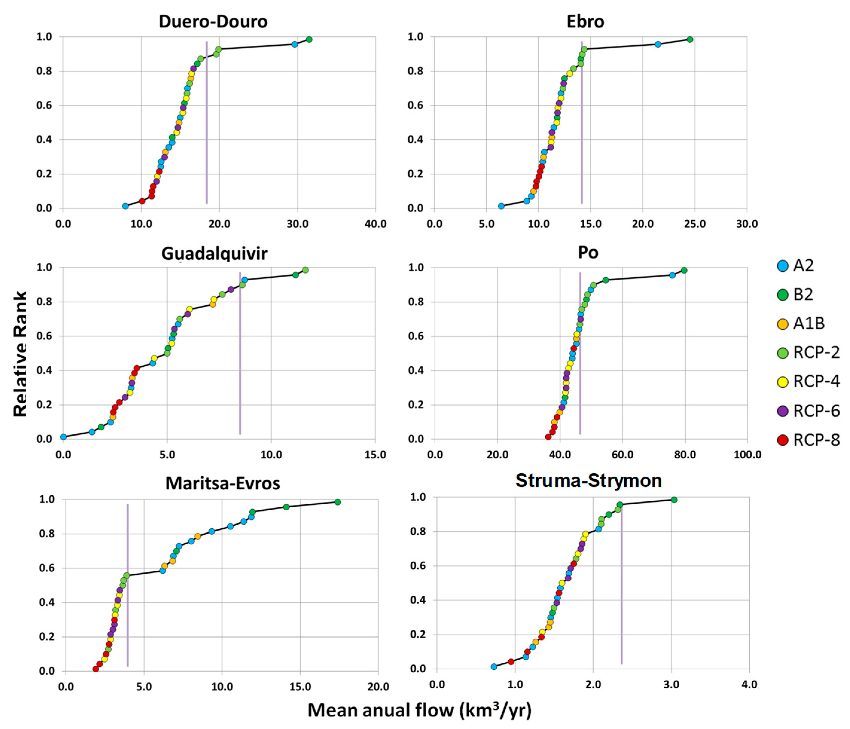
Climate forcing is assessed in
Figure 7, which shows the estimation of mean annual flow obtained in the 35 climate change scenarios for the six basins under analysis.
Figure 7 shows the ranked values of mean annual flow in the long-term projection. The vertical purple line represents the estimate of the current mean annual flow. As model estimates in the 16 runs corresponding to the current period showed a large variability, mean annual runoff values were corrected for bias in all models by using the GRDC composite runoff field, which combines observed river discharges with a water balance model [
17], and is a reference of the current global surface runoff [
30,
31]. Following González-Zeas [
31], we applied the bias-correction methodology based on the determination of a monthly correction factor. We calculated the monthly mean runoff series for the control scenario to obtain 12 representative statistical parameters, that is, the ratios between the GRDC values (observed) and the simulated runoff. These multiplying factors were used to correct bias in control and the projected series.
The results show a large uncertainty in the estimation of future mean annual flow, varying significantly from one climate model (and emission scenario) to another. As the large-scale hydrological models used in these type of studies, usually, are very simple, results incorporate an additional source of uncertainty [
1,
35,
36]. Most projections imply a reduction of mean annual flow for the six basins under study, although there is no apparent correlation between the emission scenario and the projected evolution of the mean annual flow. Our results agree with other studies that reported mean annual runoff projections [
35,
36,
37,
38,
39]. These studies provide a coherent pattern of change in the annual runoff, predicting a high degree of confidence and severe decreases (up to 40%) in surface runoff in areas already affected by water scarcity, like the Mediterranean region.
It should be noted that climate change scenarios are not only uncertain, but they have been evolving over a short period of time. Thus, strategies for water management should focus on the long-term when several dry and wet cycles periods would occur. Results also suggest that, although climate models are the most robust tools available to generate consistent climate change scenarios, they are still a source of considerable uncertainties [
40,
41]. It could be partially explained by the increase in the differences between emissions scenarios for long-term analysis. These results are consistent with several inter-comparison studies that also show considerable variability in the magnitude and timing of the projected runoff [
36,
37,
38,
39].
3.2. Risk of Water Scarcity
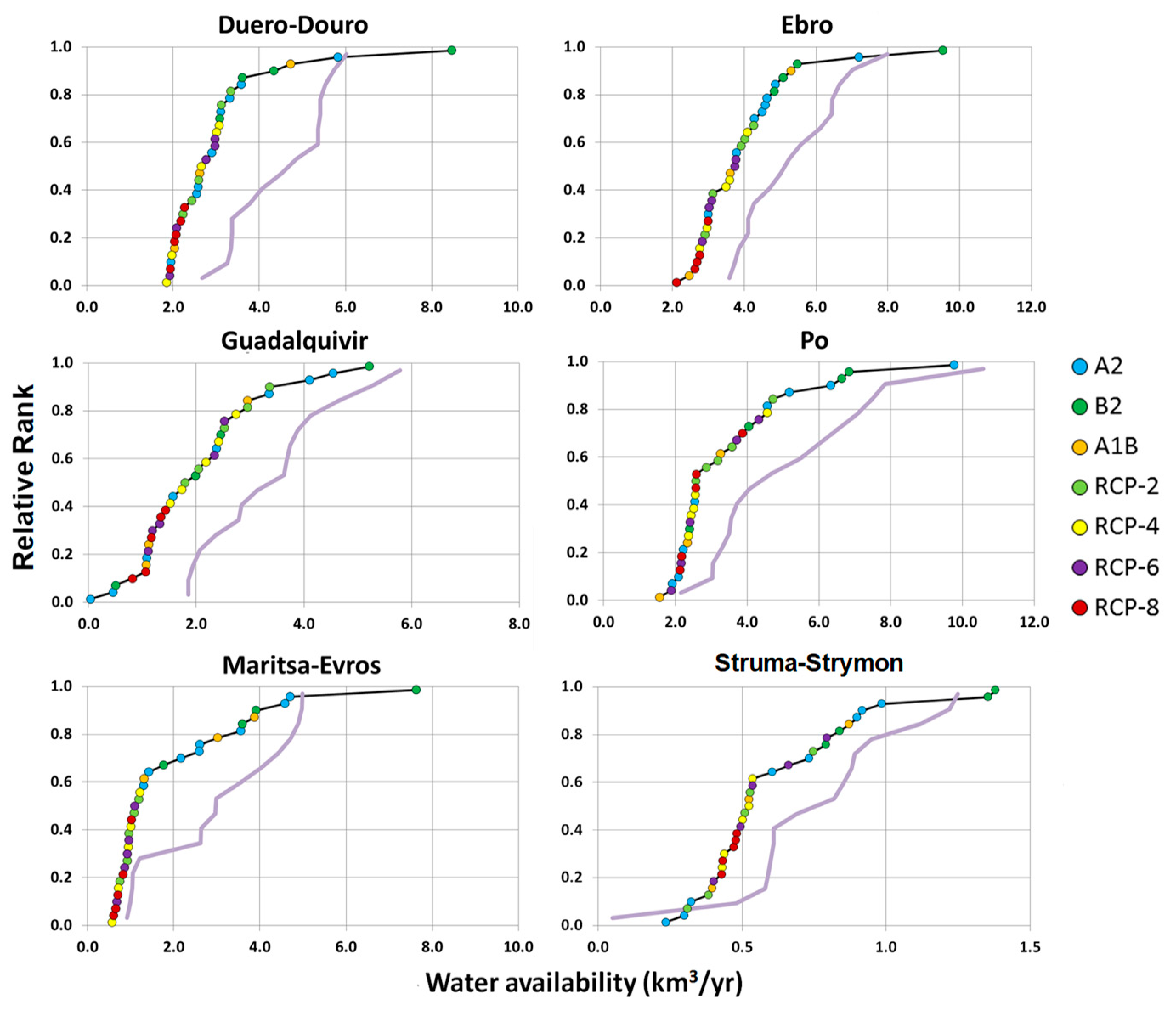
The results of potential water availability are shown in
Figure 8, which presents the ranked values of water availability in the historical period (CTL: 16 model runs; purple line) and in the long-term projection (35 model runs; black line). The uncertainty in the estimation of water availability is large, even in the historical period, where streamflow from all models has been bias-corrected to produce the same mean annual flow in each basin. It suggests that the differences in the representation of the hydrologic regimes among the models have an important influence on the potential water availability estimation. Relatively small differences in seasonality or interannual variability may produce important differences in water availability. All curves corresponding to the long-term projection of water availability are clearly to the left of the curves corresponding to the historical period, suggesting a clear signal of reduction of water availability. By comparing the range of obtained values for mean annual flow (
Figure 7, x-axis) and potential water availability (
Figure 8, x-axis), in the long-term projection, it can be seen that the range of the latter is significantly smaller. This means that the management of the reservoirs plays an important role by attenuating the hydrologic variability. Several studies agree that the propagation of the uncertainties affects water resource system performances [
42,
43,
44,
45,
46]. Thus, the uncertainty associated with the performance of a water resources system should be evaluated with extreme care.
3.3. Water Availability for Agriculture
The results obtained in the previous section suggest a significant reduction of water availability in future scenarios. In this section, we focused specifically on water availability for agriculture. We also explored possible adaptation options to face water scarcity in future scenarios. The analysis was carried out for the six basins under analysis, but only for one of the emission scenarios: A1B. We selected this emission scenario because it provides good coverage of the range of potential water availability projections in most basins. There are three models available for this emission scenario in the ENSEMBLES project: CRNM, KNMI, and ETHZ (
Table 2).
3.3.1. Future Water Availability for Agriculture
The analysis of the demand reliability curves for urban and irrigation demands for the six basins is shown in
Figure 9. The curves representing the reliability of the urban demand are presented in light colors (blue lines correspond to the historical period (1960–1990), and red lines correspond to the long-term time horizon (2070–2100)), and those representing the irrigation demand are presented in dark colors. Results show that there is a very large model uncertainty. Climate models applied in the ENSEMBLES project are known to produce strong precipitation bias in South Eastern basins [
47]. Although streamflow series were corrected for observed bias in the control period, the produced results might be misleading in terms of water availability due to the strong bias correction performed. Of the three models analyzed, CRNM provides the lowest values of water availability, except for the Po basin. The urban required reliabilities (98%) are represented by light dotted horizontal lines. The reliabilities of the irrigation demand for the demand values equal to water availability are highlighted by dark-colored horizontal lines. The reliability of the urban demand is the factor limiting the irrigation water availability when these reliabilities are higher than the minimum required reliability for irrigation (90%). This means that a correlative action to improve the efficiency of urban water use would have a beneficial effect on water availability for irrigation. The values of water availability for irrigation demand are marked with vertical lines and summarized in
Table 3. For instance, if we focus on Struma-Strymon basin and the KNMI model, only 13% effort is required because the potential water availability for the historical period (blue line) and for the long-term time horizon (red line) are similar. The effort needed is much larger in Guadalquivir than in the other five basins (the difference between red and blue vertical lines).
Results show that there is a very large model uncertainty. Of the three models analyzed, CRNM provides the lowest values of water availability, except for the Po basin. The model ETHZ provides the largest values of water availability, except for the Ebro basin. According to the analysis performed, the effect of growing irrigation demand on the reliability of urban demand is apparent in all cases. Water availability for irrigation in current conditions would be limited by the reliability of supply to urban demands in all basins, at least, for one of the models analyzed. In the future scenarios, the limiting factor is the reliability of urban demands in almost all cases, suggesting that irrigation will have to face strong competition for scarce resources in the future. The distance between water availability in current and future conditions is an indicator of the intensity of climate change impacts on water resources in each basin. The basin which requires the greatest adaptation effort is the Guadalquivir basin, with projected reductions of water availability up to 75% (for KNMI model). While in the Struma-Strymon basin, the effect is relatively small, in the Guadalquivir basin, this effect is really dramatic, with a reduction from 3.2 km3/yr for current conditions to 0.85 km3/yr for the climate change scenario (for KNMI model).
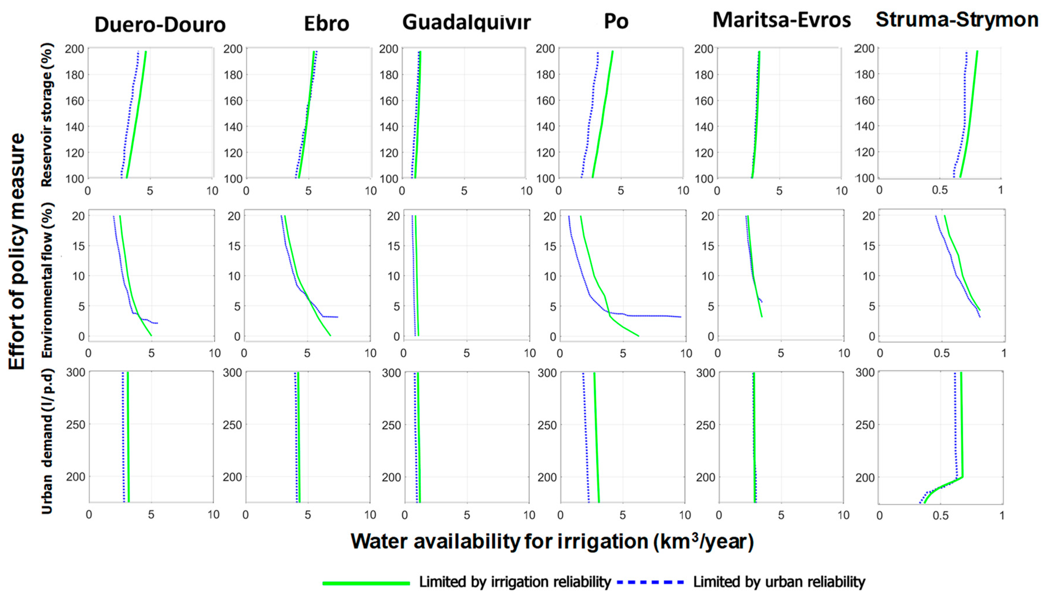
3.3.2. Effectiveness of the Policy Measures
The analysis of policy measures in the long-term horizon under emission scenario A1B is presented in
Figure 10. Results correspond to the model KNMI, which provides intermediate values for projected water scarcity. The analysis for reservoir storage was performed by increasing the capacity of existing reservoirs in the basins progressively (in 15 stages), from 100% to 200% of current value, and repeating the analysis of the demand reliability curve for each stage. The analysis of environmental flow modification was performed by considering ecological flows ranging from the 20% percentile of the marginal distribution of monthly flows to 0%, in seven stages. The reference situation assumed for the control scenario is 10%, so in this case, the policy might increase or decrease water availability with respect to current conditions. The analysis for urban demand efficiency was performed by considering diminishing values of the maximum allowable per capita urban demand. The starting value was 300 l/pd and was reduced to 175 l/pd in six stages.
The upper row of
Figure 10 shows the results for the analysis of increased reservoir storage in the six basins. The center row shows the results for the analysis of environmental flow allocation, and the bottom row shows the results of the analysis of the increased efficiency of urban water use. The plots show the irrigation demand for the limiting reliability of urban supply (dashed blue) and irrigation (green) as a function of the corresponding variables: percentage of reservoir storage in the basin, the percentile of the monthly distribution for environmental flows, and per-capita consumption for urban demand. Water availability is determined for the most restrictive of both conditions. For this model, the reliability of urban demand is the limiting condition in most cases. To facilitate comparison, the scale of the water availability for irrigation has been unified in all plots, except for the case of Struma-Strymon, which is a small basin. The slopes of the curves show the relative sensitivity of the different basins to the measures under analysis. In the case of storage, the Guadalquivir basin is the least sensitive because it already has a very large reservoir capacity compared to its mean annual flow. The Ebro, Po, and Struma-Strymon basins show the largest sensitivities. In the case of environmental flows, the Guadalquivir basin shows again the least sensitivity. Water availability could not be significantly increased even if environmental flows were reduced to zero. This is because the hydrologic regime is very irregular, and the low percentiles of the monthly distribution correspond to very small values. In the other basins, the sensitivity is very large, particularly if environmental flows are reduced with respect to current allocation. In the case of efficiency of urban water use, the sensitivity is very small in all cases because urban demand is only a small fraction of irrigation demand.
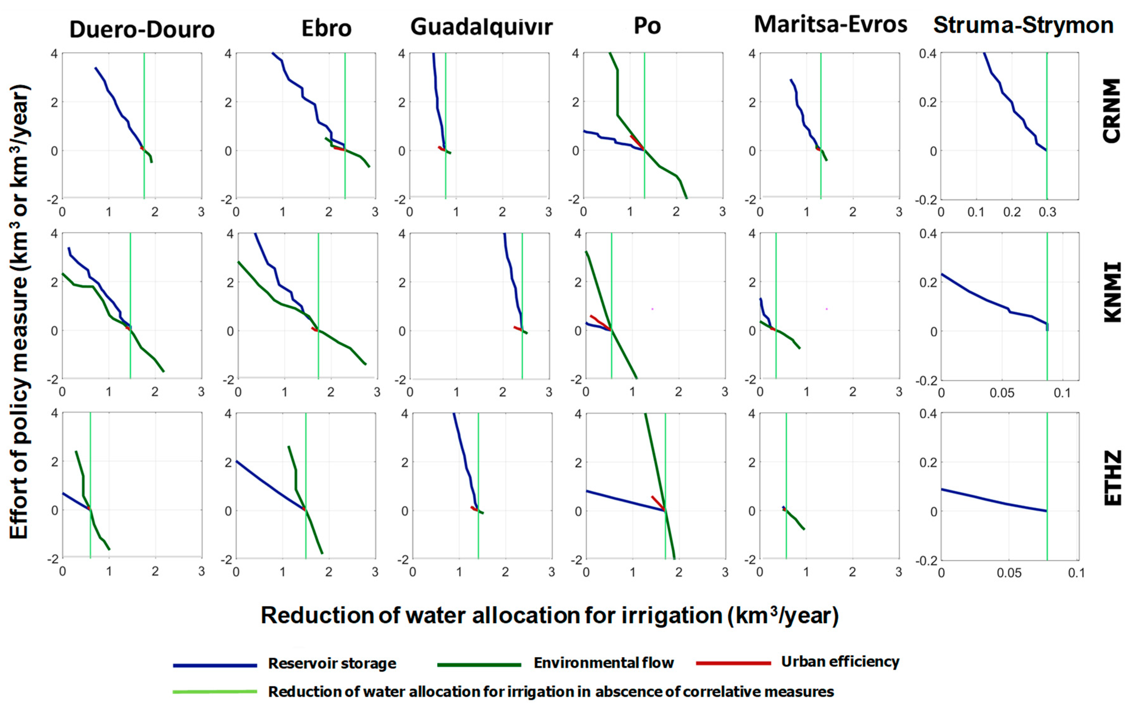
3.3.3. Trade-offs of the Policy Measures
The comparative trade-off analysis for the six basins is presented in
Figure 11. The plots present the required reduction of water allocation to irrigation as a function of the application of correlative policies: increased storage (blue), reduction of environmental flow allocation (green), and increased efficiency in urban supply (red). In order to allow for comparisons, we used a common system of units for all correlative policies, based on the added storage volume, in km
3, or in the change of the water allocated to environmental use (in km
3/yr) or in the water savings released from urban allocation (in km
3/yr). The scale of the reduction of water allocation is unified in all plots, except in the case of Struma-Strymon. The required adaptation effort in the absence of correlative measures is marked by the light green line.
The plots correspond to the most limiting case between urban and irrigation demands. The lines correspond to the evolution of the required adaptation effort as a function of the intensity of the application of the policy. The policy objective (adequate supply reliability) can be achieved with several strategies: only through demand reduction (horizontal), only through the combined policy (vertical), or through a combination of both. Through this Figure, we may evaluate the intensity, range, and efficiency of the measure. The intensity (effort) corresponds to the degree of implementation of the policy measure that would be required to avoid demand reduction entirely. It is represented by the value corresponding to the point at which the line (corresponding to any policy measure) crosses the vertical axis (and corresponds to zero reduction of water allocation for irrigation). For instance, a reduction of 2.2 km3/yr on environmental flows would avoid demand reductions in Duero-Douro basin (KNMI model). The range is determined by the length of the projection of the entire line on the horizontal axis. This represents the maximum extent to which the reduction can be avoided if the maximum intensity of the policy measure was applied. For instance, for the Duero-Douro basin and the KNMI model, the range corresponding to the reservoir volume measure goes from 1.4 km3/yr of reduction of water allocation for irrigation (current reservoir volume is maintained in the future) to 0.1 km3/yr of water reduction when the policy action is applied at the maximum intensity analyzed (by increasing the capacity of existing reservoirs to 200% of current value, 3.2 km3). Otherwise, if the CRNM model is selected (Duero-Douro basin), the effectiveness of the three correlative policies is very similar because the three lines are almost superimposed. However, the range is very different. The range of urban use efficiency is very small compared to the amount of irrigation demand that has to be reduced. The range of storage increment is also limited, especially if we account for the fact that storage has been doubled in our analysis. The Guadalquivir basin is significantly different because the little scope for action and the very high slope of the lines imply that the only possible adaptation measure among those considered in this study is the reduction of the irrigation demand. The range also indicates to what extent the proposed measure can be implemented. While there is no limit for the increase in reservoir storage, both the improvement of urban use efficiency and the reduction of allocation to environmental flows clearly have a limit. In many cases, full avoidance can be achieved through the range of values analyzed for the policy measures, but in other cases, the lines do not reach the vertical axis, meaning that reduction cannot be fully avoided. This is the case of increased urban water use efficiency, which can only avoid a small fraction of the reduction. The efficiency is represented by the inverse of the slope of the lines, which describes the ratio between the policy result (horizontal axis) and the policy effort (vertical axis). Vertical lines are inefficient because a large effort in policy would be required to produce a comparatively small result. Conversely, lines with small slopes represent very effective policies because a small policy effort would produce a comparatively large result. This effectiveness is formulated regardless of the cost of the measures, which is outside the scope of this work.
The analysis of
Figure 11 shows that the intensity, range, and effectiveness of policy measures varies not only across basins in response to different configurations but also across models, in response to different climate change scenarios. In general, the model, which yielded the greatest adaptation effort, is CRNM and the basin with greatest adaptation effort is the Guadalquivir basin.
Overall, the policy option that has the greatest impact on irrigation demand reduction is the water allocation to environmental flows. We can see that moving the values of required environmental flows in the range from the 5% to 15% percentile, very significant changes can be obtained for the required reduction of irrigation demand. It should be noted that, although the environmental flows have been proved to have important ecological benefits [
48], their implementation also involves significant economic costs [
49]. Thus, in-depth analyses from both an environmental and economic perspective are suggested, since it may have a very significant impact on future water availability.
4. Conclusions
Most of southern Europe is expected to be exposed to greater water scarcity and pressure on water resources, increased water demand, and a higher allocation of water to environmental purposes, leading to a narrow margin to improve water availability in the near future. As proposed by Garrote [
1], successful adaptation measures should be able to anticipate these negative effects of climate change and to provide the ability to progressively adapt to the situation as it evolves. In this study, we showed that, although the effects of climate change on potential water availability could be significant, the application of adaptation policies for water resources management could play a transcendental role in mitigating them. For instance, for the Duero-Douro basin and the KNMI model, the range corresponding to the reservoir volume measure goes from 1.4 km
3/yr of reduction of water allocation for irrigation (current reservoir volume is maintained in the future) to 0.1 km
3/yr of water reduction when the policy action is applied at the maximum intensity analyzed (by increasing the capacity of existing reservoirs to 200% of current value, 3.2 km
3). We showed the interdependence between the different demands, meaning that if specific measures oriented to improve the urban water use efficiency were implemented, a correlative improvement of the irrigation water availability could be achieved. In this study, the potential improvement of the irrigation water availability ranged between 0 (Maritsa-Evros basin) and 0.7 km
3/yr (Po basin). Thus, the inclusion of adaptation policy measures in river basin management plans is a key factor to face the effects of long-term climate change.
Most climate change scenarios suggest a reduction of mean annual flow for the six basins under study, although our results highlighted large uncertainties in the estimation of future mean annual flow and potential water availability. These uncertainties are not only a consequence of the wide range of emission scenarios analyzed but also of the different climate models used for the projection. The ratio between the future mean annual flow difference among climate change scenarios and the mean annual flow in the historical period ranged between approximately 1 (Duero-Douro, Ebro, Po, Struma-Strymon) and 3.5 (Maritsa-Evros). Adaptation policies should acknowledge these uncertainties identifying adaptive pathways that can be effective in a wide range of climate change scenarios. By comparing the impact of the three correlative policy measures analyzed to diminish the need of decreasing the irrigated area (reference policy), the environmental flow requirements showed the greatest sensitivity, suggesting that the trade-off between water availability and environmental flow allocations should be further analyzed. For instance, in the Duero-Douro basin, a variation (positive or negative) of 1 km3/yr of environmental flows requirements implied a variation up to 0.6 km3/yr of water availability for irrigation. The effectiveness of the development of additional storage capacity was found to be very sensitive to local conditions and hydrologic regime. For some basins, like Po or Struma-Strymon, additional storage may significantly increase water availability, that is, an increase of 1 km3 of reservoir capacity implied and increase up to 2 km3/yr of water availability for irrigation. In other basins, like Guadalquivir, doubling current storage will only slightly improve water availability. Improving urban water use efficiency will also improve water availability for irrigation, but the margin for action is limited (ranging between 0 and 0.4 km3/yr) because urban demands are only a small fraction of water consumption in the region. Finally, it should be noted that, although the methodology and analysis were performed on six representative basins, the study should be extended to other basins in order to validate our results and conclusions for entire southern Europe.

 ,
, 


