GIS Applications to Investigate the Linkage between Geomorphological Catchment Characteristics and Response Time: A Case Study in Four Climatological Regions, South Africa

Abstract

In flood hydrology, geomorphological catchment characteristics serve as fundamental input to inform decisions related to design flood estimation and regionalization. Typically, site-specific geomorphological catchment characteristics are used for regionalization, while flood statistics are used to test the homogeneity of the identified regions. This paper presents the application and comparison of Geographical Information Systems (GIS) modelling tools for the estimation of catchment characteristics to provide an enhanced understanding of the linkage between geomorphological catchment characteristics and response time. It was evident that catchment response variability is not exclusively related to catchment area, but rather associated with the increasing spatial–temporal heterogeneity of other catchment characteristics as the catchment scale increases. In general, catchment and channel geomorphology overruled the impact that catchment variables might have on the response time and resulting runoff. Shorter response times and higher peak flows were evident in similar-sized catchments characterized by lower shape factors, circularity ratios, and shorter centroid distances and associated higher elongation ratios, drainage densities and steeper slopes. The GIS applications not only enabled the inclusion of a more diverse selection of catchment characteristics as opposed to when manual methods are used, but the high degree of association between the different GIS-based methods also confirmed their preferential use.

1. Introduction

In flood hydrology, geomorphological catchment characteristics serve as fundamental input to inform decisions related to design flood estimation and hydrological regionalization. In essence, the main objective of regionalization in flood hydrology is to improve and augment the accuracy of design flood estimates at gauged and ungauged sites, which is normally reflected by the Goodness-of-Fit (GOF) statistics of regionalized equations compared with those at a single site [1]. The two most difficult aspects of any regionalization process are [2,3]: (i) to establish whether regionalization is actually required, and (ii) to identify and establish the number of homogeneous hydrological regions required. In using regionalization methods, e.g., residual [3], clustering [4] and/or region-of-influence (ROI) [2,5] methods, the variables and/or parameters are normally selected to define pair-wise similarity or dissimilarity of catchments in a particular region. Typically, geomorphological catchment characteristics at specific sites are used for regionalization, while flood statistics (e.g., L-moment ratios and other statistical measures from observed rainfall-runoff data) are used to test the homogeneity of the identified regions. Hence, geomorphological catchment characteristics and the accurate estimation thereof are essential to both regionalization procedures and the actual estimation of design floods, i.e., flood events characterized by a specific magnitude and annual exceedance probability (AEP).

Despite the fact that geomorphological catchment characteristics serve as fundamental input to inform decisions related to design flood estimation and regionalization, manual methods and map sheets are still often used to estimate these geomorphological catchment characteristics [6,7]. This is particularly the case in South Africa and, in general, the inherent human and instrumentation errors associated with such manual data acquisition processes, linked to the time taken to extract the information, limit the number of catchment parameters being considered by researchers when undertaking multiple regression analysis and regionalization procedures to describe the linkage between geomorphological catchment characteristics and other flood indices.

Apart from the limited number of geomorphological catchment characteristics being considered, differences in catchment parameter estimations using manual and automated methods are also to be expected. For example, Cleveland et al. [8] acknowledged the qualitative similarity between manual and automated measures of geomorphological catchment characteristics, but also stressed that the relative differences in estimating these characteristics are statistically significant. Fang et al. [9] also established average relative differences up to 15% between manual and automated catchment parameter estimation methods. In contrast, Keshtkaran and Sabzevari [10] gave preference to manual catchment parameter estimation methods to conduct regression analyses to ultimately estimate runoff using a geomorphological instantaneous unit hydrograph (GUIH) approach. However, differences between the various geomorphological catchment characteristics estimated using manual and automated methods varied between 5% and 41%, while in comparison to the observed flood events, the flood estimates based on the manual input were on average 10% less accurate than those estimates based on the automated input.

Currently, with the availability of Geographical Information Systems (GIS), which has encompassed almost every field in the engineering and natural sciences; accurate, efficient and consistent methods are available to estimate geomorphological catchment characteristics. GIS has been widely used in several geomorphological, flood management, and environmental studies (e.g., [11,12,13]). Comprehensive sets of spatial and hydrological tools are available in both commercial, e.g., ArcGIS^TM [14] and open-source, e.g., GRASS [15] and QGIS [16] software packages. Jena and Tiwari [17] also highlighted that the use of GIS software will not only improve catchment parameter estimations but will also contribute towards objective and consistent hydrological assessments.

The complex linkage between geomorphological catchment characteristics and hydrological processes are well known and described ever since the existence and study of geomorphological and hydrological sciences, e.g., Rodríguez-Iturbe and Valdés [18]. However, in order to understand and/or describe these linkages, the impact of different time and spatial scales must clearly be understood. In general, individual flood events can have dramatic effects on catchment characteristics, e.g., erosion and sediment transport; however, catchment characteristics could be regarded as constant for the purpose of hydrological prediction, while runoff generation is primarily influenced by the spatial and temporal variability of rainfall and the hydrological response of a catchment [19]. In turn, the hydrological response or catchment response time is directly related to, and influenced by the complex interaction between the spatial–temporal variability of rainfall and heterogeneous catchment characteristics, e.g., catchment geomorphology, channel geomorphology, and various other catchment variables [20].

Frequently, the large variability in the hydrological response of catchments to extreme rainfall is not entirely reflected in the current design flood estimation methods; hence, design floods are often over- or underestimated and, subsequently, the resultant failure of hydraulic structures, e.g., culverts, bridges, and spillways, is inevitable [21]. A given runoff volume may or may not represent a flood hazard or result in the possible failure of hydraulic structures, since hazard is dependent on the magnitude and temporal distribution of runoff [3,22]. Consequently, most hydrological analyses of rainfall and runoff to determine hazard or risk, i.e., design flood estimation, especially in ungauged catchments, require the estimation of catchment response time parameters, e.g., the time of concentration (T_C), lag time (T_L) and/or time to peak (T_P), as primary input. Bondelid et al. [23] and Gericke and Smithers [24] showed that more than 75% of the total error in design flood estimates in ungauged catchments could be ascribed to errors in the estimation of catchment response time parameters.

Empirical methods are the most frequently used to estimate the catchment response time in ungauged catchments and represent 95% of all the methods used internationally [24]. In using empirical methods, observed time parameters are normally related to rainfall–runoff variables and geomorphological catchment characteristics using multiple regression analysis to transfer knowledge from gauged to ungauged sites. However, significant relationships are not always evident, which emphasizes the complexities of runoff generation and the need to consider individual catchment processes as part of a conceptual framework, rather than as single processes in isolation. Typically, a simplified conceptual framework will include [25]: (i) rainfall as the primary input, (ii) geomorphological catchment characteristics acting as a buffer and transfer function, and (iii) direct runoff as the output.

Catchment area is often recognized as a geomorphological ‘transfer function’ of hydrological significance having a large influence on many flood indices affecting the catchment response time and resulting runoff [26,27,28]. Klein [29] regarded 300 km² as the upper area limit for ‘small’ catchments characterized by more rapid catchment responses as opposed to larger catchments with longer and more attenuated hydrographs. However, it was also acknowledged that the differences between the two catchment scales may be due to differences in the dominating catchment response mechanisms, i.e., overland flow response in small catchments and channel flow response in larger catchments. In addition to catchment area, other geomorphological catchment characteristics such as shape, hydraulic and main river lengths, average catchment and main river slopes, and drainage density are also regarded as important [20,30,31].

Catchment variables, e.g., land-use, vegetation and soils also have an influence on the response of a catchment. According to Gericke and Smithers [25], the nature and spatial distribution of main land-use groups (e.g., urban, rural, waterbodies and local geology) at a catchment level affect the temporal and spatial distribution of runoff. Typically, in urbanized areas, the landcover is transformed from pervious to impervious, while the topography (e.g., catchment slope) is changed irreversibly through the removal of surface depressions. Consequently, reduced infiltration and groundwater recharge potential are evident, while the runoff potential increases [25]. The influence of natural vegetation on the peak flow and volume of runoff depends on the climatological region in which a particular catchment is situated, with vegetation normally dampening the effect of spatial rainfall on runoff in humid temperate catchments [25,32,33]. Pechlivanidis et al. [34] highlighted that the spatial variability of antecedent soil moisture conditions has a strong influence on runoff, with dominant flow paths varying according to the soil moisture conditions and consequently affecting the peak flow and catchment response time. In considering the increase in heterogeneity associated with landcover, vegetation, land-use treatment strategies, and soils as the catchment scale increases, it is evident that the catchment response time will also be more variable and most likely be influenced by a combination of these catchment variables. Hence, common practice in flood hydrology is to group all these catchment variables together using a weighted Curve Number (CN) approach in order to reflect the impact of these variables on catchment response time and other flood indices [35].

Given the sensitivity of runoff generation mechanisms to catchment response time, which is in turn influenced by the catchment characteristics, the linkage between geomorphological catchment characteristics and response time is evident and the need for accurate catchment parameter estimation methods is highlighted to ultimately enable the successful deployment of any hydrological analysis and/or regionalization scheme. Thus, the primary objective of this paper is to demonstrate and compare the application of both specialized GIS spatial modelling tools and conventional equations in conjunction with standard GIS tools in an ArcGIS^TM environment to estimate a selection of geomorphological catchment characteristics which could have a direct influence on catchment response time and runoff generation. Sixty-five ‘medium-to-large’ gauged catchments (>100 km²), located in four distinctive climatological regions of South Africa, are used in this case study to investigate the linkage between geomorphological catchment characteristics and observed catchment response time by evaluating the individual and combined influences of catchment geomorphology, channel geomorphology and catchment variables on response time and runoff generation.

The next section provides a general overview of the study area. Thereafter, the methodologies involved in meeting the objectives are detailed, followed by the results, discussion and conclusions.

2. Study Area

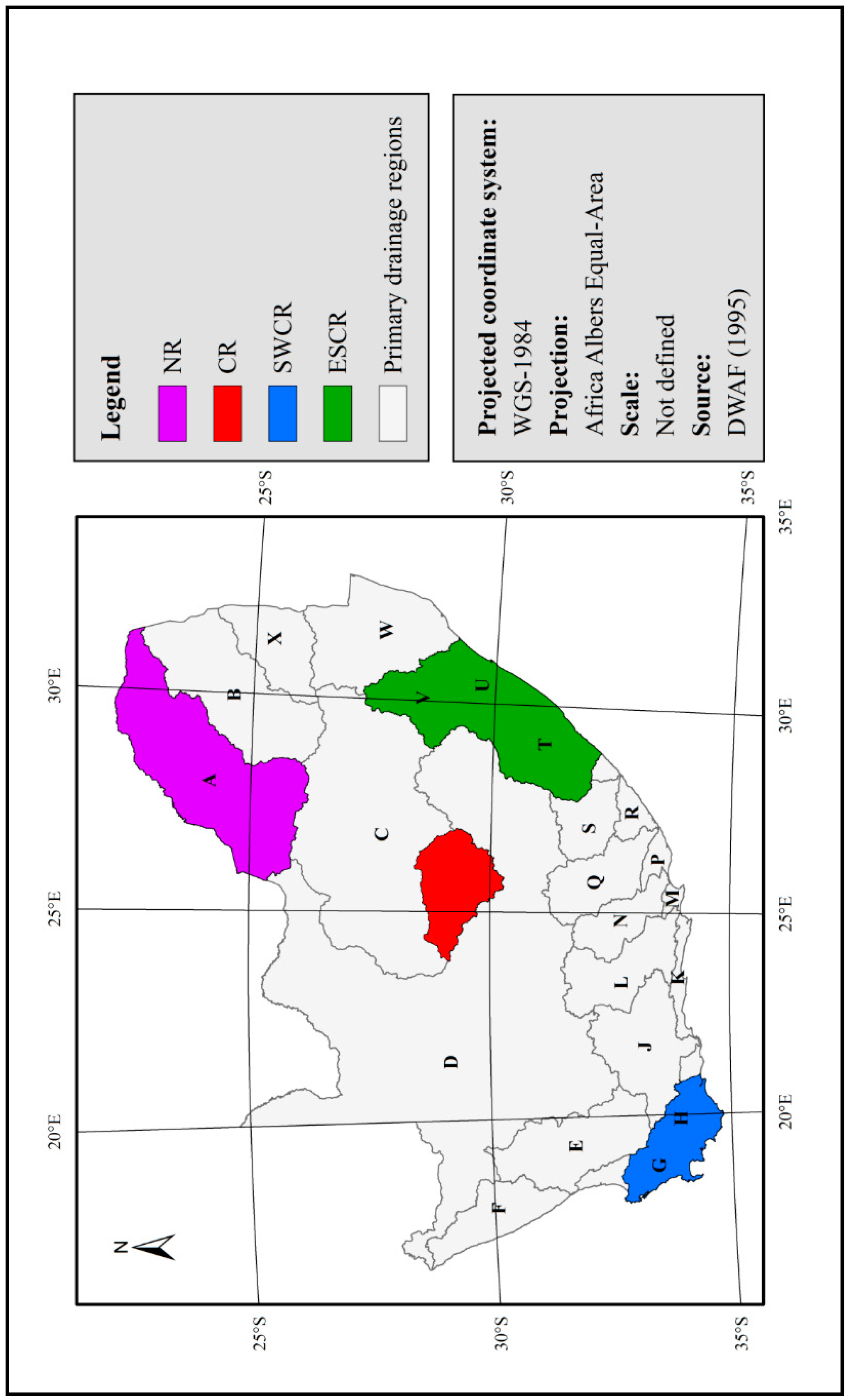
South Africa is located on the most southern tip of Africa and divided into 22 primary drainage regions (A to X) as shown in Figure 1. These primary drainage regions are further delineated into 148 secondary drainage regions, i.e., A1, A2, to X4 [25,36,37]. The 65 gauged catchments are located in 26 of these secondary drainage regions which form part of four distinctive climatological regions of South Africa, i.e., the Northern Region (NR), Central Region (CR), Southern Winter Coastal Region (SWCR), and Eastern Summer Coastal Region (ESCR).

The four climatological regions are representative of the broad variations in climate (e.g., Mean Annual Precipitation (MAP), rainfall type, distribution and rainfall seasonality), catchment geomorphology, channel geomorphology, geographical location, and altitude above mean sea level (MSL) found in South Africa [25]. The catchment areas range between 103 and 33,300 km² and are regarded as ‘gauged’, since Department of Water and Sanitation (DWS) flow-gauging stations are located at the outlet of each catchment.

Table 1. Main properties of the 65 catchments located in the four climatological regions (after [38]).

Range Descriptors	Climatological Regions
	NR	CR	SWCR	ESCR
Secondary drainage regions	A2, A3, A5–A7 and A9	C5	G1, G4, H1–H4, H6 and H7	T1, T3–T5, U2, U4, V1–V3 and V5–V6
Number of catchments	16	15	12	22
Catchment area (km2)	103–23,852	185–33,278	109–2878	129–28,893
Altitude above MSL (m)	544–1763	1021–2120	86–2060	31–3149
Average catchment slope (%)	3–18	2–7	16–42	11–34
MAP (mm)	429–1175	430–648	267–1132	773–1265
Rainfall season	Summer	Summer	Winter	All-year

contains a summary of the main catchment properties in each climatological region under consideration. The DWS flow-gauging station numbers are used as catchment descriptors for easy reference in all the subsequent tables and figures.

3. Methods

3.1. Estimation of Catchment Characteristics

The majority of the original GIS data feature classes (e.g., points, lines and polygons) applicable to South Africa were obtained from the DWS. This was followed by the extraction and transformation of the data to a projected coordinate system applicable to each catchment in the four climatological regions. Transformation to a projected coordinate system portrays the curved surface of the earth on a flat surface, during which, the distance, area, shape, direction or a combination thereof might be distorted. The Albers Equal-Area coordinate reference system, suitable for South Africa, was preferred, since this conic projection uses two standard parallels to reduce some of the distortion of a projection with one standard parallel. Although neither shape nor linear scale is truly correct, the distortion of these properties is minimized in the region between the standard parallels. All areas are proportional to the same areas on the earth, while distances are most accurate in the middle latitudes. The standard parallels were established by using the one-sixth rule by determining the range in latitude (degrees) north to south divided by six. The first standard parallel is positioned at one-sixth of the range above the southern boundary and the second standard parallel is positioned at minus one-sixth of the range below the northern boundary [39].

3.1.1. Catchment Geomorphology

The Shuttle Radar Topography Mission (SRTM) Digital Elevation Model (DEM) for Southern Africa at a 30-m resolution [40] was prepared for the study area. The Hydrology toolset contained in the Spatial Analyst Tools toolbox of ArcGIS^TM was used to prepare a hydrologically corrected and depressionless DEM. In other words, all ‘sinks’, i.e., cells with a lower elevation compared to the surrounding cells, were filled to generate continuous flow direction and flow accumulation rasters for the identification of catchment areas for specified pour points located at the catchment outlet. The hydrologically corrected DEM was subsequently projected and transformed to enable the estimation of geomorphological catchment characteristics, area (A), perimeter (P), hydraulic length (L_H), centroid distance (L_C), and average slope (S).

The hydraulic length (L_H), i.e., the distance measured along the longest river from the catchment outlet to the catchment boundary upstream of the fingertip tributary, was estimated using the Longest Flow Path tool in the Hydrology toolset. The Mean Center tool in the Measuring Geographic Distributions toolset contained in the Spatial Statistics Tools toolbox was used to estimate the centroid of each catchment. The centroid distance (L_C), i.e., the distance along the main river between the outlet and the point on the main river closest to the centroid of the catchment, was established by using the Measure tool in ArcMap [7,14].

In addition to the above-mentioned parameters, i.e., P, L_H and L_C, the catchment shape was also estimated in terms of a shape factor, and circularity and elongation ratios using Equations (1) to (3), respectively [17,28]:

$$F_S={\left(L_H{L}_C\right)}^{0.3},$$

(1)

$$R_C=\frac{P}{{\left(4\pi A\right)}^{0.5}},$$

(2)

$$R_E=\frac{2}{L_H}{\left(\frac{A}{\pi }\right)}^{0.5},$$

(3)

where F_S is the shape factor, R_C is the circularity ratio, R_E is the elongation ratio, A is the catchment area (km²), L_C is the centroid distance (km), L_H is the hydraulic length (km), and P is the catchment perimeter (km).

The average catchment slope of the individual catchments was estimated using the Empirical method (Equation (4); [35]) with GIS-based input parameters and the Average Maximum Technique (Equation (5); [14]), which is the standard slope algorithm used in ArcGIS^TM. In the case of Equation (5), a slope raster was generated from the DEM using the Slope tool available from the Surface toolset contained in the Spatial Analyst Tools toolbox.

$$S_1=\frac{M\Delta H}{10A},$$

(4)

$$S_2=100\sqrt{{\left(\frac{\Delta z}{\Delta x}\right)}^2+{\left(\frac{\Delta z}{\Delta y}\right)}^2},$$

(5)

$$\frac{\Delta z}{\Delta x}=\left[\frac{\left(C_3+2C_6+C_9\right)-\left(C_1+2C_4+C_7\right)}{\left(N{x}_c\right)}\right],$$

(5a)

$$\frac{\Delta z}{\Delta y}=\left[\frac{\left(C_7+2C_8+C_9\right)-\left(C_1+2C_2+C_3\right)}{\left(N{y}_c\right)}\right],$$

(5b)

where S_1,2 is the average catchment slope (%), A is the catchment area (km²), ΔH is the contour interval (m), M is the total length of all contour lines within the catchment (km), Δz/Δx is the rate of change of the slope surface in an east-west direction from the center cell, C₅ (m·m⁻¹), Δz/Δy is the rate of change of the slope surface in a north-south direction from the center cell, C₅ (m·m⁻¹), C₅ is the center cell, C_{1–4 & 6–9} are the surrounding cells, N is the number of grid points or cells (8), x_c is the east-west cell size, and y_c is the north-south cell size.

3.1.2. Channel Geomorphology

The length of the longest river (L_CH) was estimated using the Longest Flow Path tool in the Hydrology toolset, and the longitudinal profiles were obtained from the DEM using the Stack Profile tool in the Functional Surface toolset contained in the 3D Analyst toolbox. The average slope of the main rivers (S_CH) was estimated using the above GIS-based longitudinal profiles and the following methods [41,42]: (i) Equal-area (Equation (6)), (ii) 10-85 (Equation (7)), and (iii) Taylor-Schwarz (Equation (8)).

$${S_{\mathrm{CH}}}_1=\frac{\left(H_T-H_B\right)}{10L_{CH}},$$

(6)

$$A_i=\left(\frac{H_i+H_{i+1}}{2}-H_B\right)L_i,$$

(6a)

$$H_T=\frac{\left({\displaystyle \sum _{i=1}^N{A}_i\ast 2}\right)}{1000L_{CH}}+H_B,$$

(6b)

$${S_{\mathrm{CH}}}_2=\frac{\left(H_{0.85L_{CH}}-H_{0.10L_{CH}}\right)}{\left(7.5L_{CH}\right)},$$

(7)

$${S_{\mathrm{CH}}}_3={\left(\frac{10000L_{CH}}{{\displaystyle \sum _{i=1}^N\frac{L_i}{\sqrt{S_i}}}}\right)}^2,$$

(8)

where S_CH1–3 is the average main river slope (%), A_i is the incremental area between two consecutive contours (m²), H_B is the elevation at the catchment outlet (m), H_i is the specific contour interval elevation (m), H_T is the maximum elevation at the river fingertip associated with S_CH (m), H_0.10L is the elevation of the main river at length 0.10L_CH (m), H_0.85L is the elevation of the main river at length 0.85L_CH (m), L_CH is the length of the main river (km), L_i is the distance between two consecutive contours (m), and S_i is the slope between two consecutive contours (m·m⁻¹).

3.1.3. Catchment Variables

Owing to the high variability associated with the characteristics and spatial distribution of catchment variables, weighted CN values were used to group the landcover, vegetation, land-use treatment strategies, and hydrological soil groups together. The attributes of the National Landcover (NLC) database [43] were firstly reclassified in ArcGIS^TM according to the generalized CN categories (e.g., agriculture, open space, forest, disturbed land, residential, paved, and commercial industry) as proposed by [35]. Thereafter, the generalized CN categories and the taxonomical soil forms with associated hydrological soil group information were combined using the Union geoprocessing tool in ArcMap. Typically, the hydrological soil group classification [35] represents the runoff potential of soils, i.e., ranging from very permeable (Group A; final infiltration = 25 mm·h⁻¹ and permeability rate >7.6 mm·h⁻¹) to impermeable (Group D; final infiltration = 3 mm·h⁻¹ and permeability rate < 1.3 mm·h⁻¹).

3.2. Estimation of Observed Catchment Response Time

The observed catchment response times, expressed as the time to peak (T_Px), were obtained from [38] which determined the average catchment T_Px values using only observed streamflow data. The observed time to peak values for individual flood events (T_Pxi) was expressed as either the net duration of a multi-peaked hydrograph and/or estimated using triangular-shaped direct runoff hydrograph approximations [38]. The ‘average’ catchment response time (T_Px) of all the flood events considered in each catchment was estimated using a linear catchment response function, Equation (9) [38]. Equation (9) is used in this study, since in event-based design flood estimation methods, the design flood estimate is based on a single and representative catchment response time parameter, while the catchment is at an ‘average condition’ [38].

$$T_{Px}=\frac{1}{3600x}\left[\frac{{\displaystyle \sum _{i=1}^N\left(Q_{Pxi}-\overline{Q_{Px}}\right)\left(Q_{Dxi}-\overline{Q_{Dx}}\right)}}{{\displaystyle \sum _{i=1}^N{\left(Q_{Pxi}-\overline{Q_{Px}}\right)}^2}}\right],$$

(9)

where T_Px is the ‘average’ catchment time to peak based on a linear catchment response function (h), Q_Dxi is the volume of direct runoff for individual flood events (m³), $\overline{Q_{Dx}}$ is the mean of Q_Dxi (m³), Q_Pxi is the observed peak discharge for individual flood events (m³·s⁻¹), $\overline{Q_{Px}}$ is the mean of Q_Pxi (m³·s⁻¹), N is the sample size, and x is a variable proportionality ratio (default x = 1), which depends on the catchment response time parameter under consideration, i.e., T_C ≈ T_P ≈ 1 and T_L = 0.6T_C with x = 1.667.

Various forms of least square regression analysis (e.g., linear, logarithmic, exponential, power, and polynomial) were considered to correlate the observed time parameter (T_Px) values (dependent variables) and 12 individual catchment characteristics (independent variables) as listed in

Table A1. Geomorphological catchment characteristics, average hydrograph and catchment response time information in the Northern Region (after [25]).

Catchment	A2H005	A2H006	A2H007	A2H012	A2H013	A2H015	A2H017	A2H019
A (km2)	774	1030	145	2555	1161	23,852	1082	6120
P (km)	136	177	64	260	179	808	180	415
LH (km)	51	86	17	57	64	252	76	132
LC (km)	27	51	7	22	37	130	40	73
FS (Equation (1))	8.74	12.40	4.25	8.53	10.32	22.60	11.14	15.67
RC (Equation (2))	1.38	1.55	1.50	1.45	1.48	1.48	1.55	1.50
RE (Equation (3))	0.62	0.42	0.79	0.99	0.60	0.69	0.49	0.67
Σ Contours M (km)	1354	2979	548	8247	4951	73,110	4842	21,701
S1 (Equation (4), %)	3.50	5.78	7.57	6.46	8.53	6.13	8.95	7.09
S2 (Equation (5), %)	2.73	4.76	6.52	5.30	7.03	5.13	7.43	5.78
LCH (km)	48	86	17	57	57	251	76	132
SCH1 (Equation (6), %)	0.41	0.37	1.27	0.56	0.42	0.13	0.42	0.29
SCH2 (Equation (7), %)	0.44	0.39	1.47	0.69	0.52	0.19	0.49	0.36
SCH3 (Equation (8), %)	0.45	0.35	1.33	0.54	0.46	0.11	0.45	0.24
DD (km·km−2)	0.09	0.17	0.24	0.14	0.12	0.13	0.12	0.14
Dolomitic areas (%)	61.2	12.4	30.6	44.2	13.9	12.5	0.0	21.1
Weighted CN value	74.8	72.4	77.3	69.8	71.6	69.3	71.2	69.6
No. of flood events	60	100	60	70	60	15	18	60
QTx (106 m3)	2.1	8.6	0.8	17.3	6	12.6	1.4	42.3
QDx (106 m3)	1.7	6.4	0.7	11	3.9	10.7	1.2	33.5
QPx (m3·s−1)	14.7	79.8	40.2	190.9	80.3	85.8	29.6	205.1
TPx (Equation (9), h)	14.3	11.2	4.1	12.4	8	28.8	6.2	25.5
Catchment	A2H020	A2H021	A3H001	A5H004	A6H006	A7H003	A9H001	A9H002
A (km2)	4546	7483	1175	636	180	6700	914	103
P (km)	347	459	174	140	63	396	186	76
LH (km)	176	216	47	68	25	162	82	38
LC (km)	61	70	17	37	9	79	44	19
FS (Equation (1))	16.22	17.92	7.45	10.53	5.16	17.08	11.70	7.19
RC (Equation (2))	1.45	1.50	1.44	1.57	1.32	1.37	1.73	2.10
RE (Equation (3))	0.43	0.45	0.82	0.42	0.60	0.57	0.42	0.30
Σ Contours M (km)	14,174	13,131	2270	3102	665	11,629	6332	1114
S1 (Equation (4), %)	6.24	3.51	3.87	9.75	7.40	3.47	13.86	21.59
S2 (Equation (5), %)	5.31	2.85	3.13	8.73	6.32	2.71	10.17	17.47
LCH (km)	176	215	47	68	25	162	82	38
SCH1 (Equation (6), %)	0.22	0.14	0.68	0.58	0.92	0.32	0.43	1.37
SCH2 (Equation (7), %)	0.34	0.19	0.73	0.71	1.10	0.33	0.50	2.01
SCH3 (Equation (8), %)	0.20	0.13	0.72	0.59	0.92	0.34	0.34	0.89
DD (km·km−2)	0.14	0.13	0.13	0.19	0.14	0.09	0.16	0.37
Dolomitic areas (%)	0.1	7.9	79.3	0.0	0.0	0.0	0.0	0.0
Weighted CN value	70.7	69.7	68.9	63.6	61.1	61.5	68.4	68.5
No. of flood events	40	30	50	30	65	40	60	16
QTx (106 m3)	28.3	74.8	1	19.5	1.9	7.1	15.8	6.5
QDx (106 m3)	22.8	49	0.8	10.3	1.5	5.8	10.8	3.9
QPx (m3·s−1)	250	145.3	34	89.6	21.5	53.6	58.8	66.7
TPx (Equation (9), h)	24.4	79.6	3.3	19	12.4	19.9	30.2	7.5

,

Table A2. Geomorphological catchment characteristics, average hydrograph and catchment response time information in the Central Region (after [25]).

Catchment	C5H003	C5H006	C5H007	C5H008	C5H009	C5H012	C5H014	C5H015
A (km2)	1641	676	346	598	189	2366	31,283	5939
P (km)	196	145	100	122	71	230	927	384
LH (km)	71	64	41	41	24	87	326	160
LC (km)	41	29	17	22	14	45	207	81
FS (Equation (1))	10.95	9.61	7.17	7.74	5.73	11.98	28.12	17.15
RC (Equation (2))	1.36	1.58	1.52	1.40	1.45	1.34	1.48	1.41
RE (Equation (3))	0.64	0.46	0.51	0.67	0.64	0.63	0.61	0.54
Σ Contours M (km)	4009	901	386	1732	419	4757	42,538	10,575
S1 (Equation (4), %)	4.89	2.67	2.23	5.80	4.44	4.02	2.72	3.56
S2 (Equation (5), %)	3.90	2.02	1.75	4.83	3.66	3.28	2.13	2.77
LCH (km)	71	64	40	41	24	87	326	160
SCH1 (Equation (6), %)	0.23	0.24	0.30	0.41	0.55	0.21	0.10	0.11
SCH2 (Equation (7), %)	0.26	0.27	0.34	0.48	0.60	0.27	0.10	0.14
SCH3 (Equation (8), %)	0.24	0.28	0.34	0.46	0.62	0.23	0.09	0.11
DD (km·km−2)	0.23	0.18	0.19	0.17	0.19	0.18	0.11	0.20
Dolomitic areas (%)	0.0	0.0	0.0	0.0	0.0	0.0	0.0	0.0
Weighted CN value	68.0	73.6	73.4	67.3	67.1	67.3	68.8	69.8
No. of flood events	101	14	91	112	13	68	28	90
QTx (106 m3)	2.1	1.4	1.2	2.2	1	3.3	46.7	23.3
QDx (106 m3)	1.7	1.3	1	2	0.8	2.3	36.5	21
QPx (m3·s−1)	32.8	36	28	44.7	14.3	41.5	168.3	203.1
TPx (Equation (9), h)	11.1	8.2	7.2	10.5	12.7	11.9	56.6	25
Catchment	C5H016	C5H018	C5H023	C5H035	C5H039	C5H053	C5H054
A (km2)	33,278	17,361	185	17,359	6331	4569	687
P (km)	980	730	65	730	411	329	146
LH (km)	378	375	29	373	187	120	68
LC (km)	230	174	17	173	103	56	33
FS (Equation (1))	30.33	27.83	6.48	27.72	19.28	14.05	10.07
RC (Equation (2))	1.52	1.56	1.35	1.56	1.46	1.37	1.57
RE (Equation (3))	0.54	0.40	0.52	0.40	0.48	0.64	0.44
Σ Contours M (km)	44,532	19,437	764	19,437	10,766	9064	933
S1 (Equation (4), %)	2.68	2.24	8.28	2.24	3.40	3.97	2.72
S2 (Equation (5), %)	2.09	1.72	7.09	1.72	2.65	3.08	2.07
LCH (km)	378	375	29	373	187	119	67
SCH1 (Equation (6), %)	0.11	0.08	0.52	0.08	0.09	0.15	0.25
SCH2 (Equation (7), %)	0.10	0.08	0.58	0.08	0.13	0.18	0.26
SCH3 (Equation (8), %)	0.09	0.08	0.60	0.08	0.10	0.16	0.28
DD (km·km−2)	0.10	0.09	0.20	0.09	0.20	0.21	0.18
Dolomitic areas (%)	0.0	0.0	0.0	0.0	0.0	0.0	0.0
Weighted CN value	69.0	70.1	67.9	70.1	69.8	69.8	73.6
No. of flood events	40	50	58	20	56	65	60
QTx (106 m3)	31	22.8	0.8	10.8	34	8.3	1.3
QDx (106 m3)	27	19.7	0.6	9.1	29.2	5.7	0.8
QPx (m3·s−1)	105.6	105	15.6	58.9	136.2	93.1	21.3
TPx (Equation (9), h)	65.6	39	9.8	40.7	55.7	16.4	8.7

,

Table A3. Geomorphological catchment characteristics, average hydrograph and catchment response time information in the Southern Winter Coastal Region (after [25]).

Catchment	G1H002	G1H007	G1H008	G4H005	H1H003	H1H006
A (km2)	186	724	394	146	656	753
P (km)	65	128	93	60	130	135
LH (km)	28	56	26	30	39	47
LC (km)	13	29	6	14	22	30
FS (Equation (1))	5.91	9.16	4.49	6.15	7.62	8.80
RC (Equation (2))	1.34	1.35	1.32	1.41	1.43	1.38
RE (Equation (3))	0.55	0.55	0.87	0.46	0.74	0.66
Σ Contours M (km)	3781	11,768	4446	1789	6969	9968
S1 (Equation (4), %)	40.74	32.52	22.58	24.55	21.26	26.49
S2 (Equation (5), %)	33.53	26.21	18.89	20.71	16.41	21.20
LCH (km)	28	55	26	29	38	46
SCH1 (Equation (6), %)	4.05	0.41	1.37	1.06	0.73	1.05
SCH2 (Equation (7), %)	4.49	0.46	1.61	1.58	0.89	0.96
SCH3 (Equation (8), %)	2.95	0.29	1.04	0.17	0.68	0.74
DD (km·km−2)	0.22	0.21	0.21	0.20	0.17	0.18
Dolomitic areas (%)	0.0	0.0	0.0	0.0	0.0	0.0
Weighted CN value	59.2	61.5	67.9	64.1	67.4	66.5
No. of flood events	90	75	75	55	72	90
QTx (106 m3)	8.1	50.4	12.2	15.8	15.1	25.9
QDx (106 m3)	5.8	43.9	8.5	12.5	11.6	18.1
QPx (m3·s−1)	123.8	238.9	139.5	79.7	115	273.6
TPx (Equation (9), h)	6.4	37.1	10.8	32.4	21.2	15.1
Catchment	H1H018	H2H003	H3H001	H4H006	H6H003	H7H003
A (km2)	109	743	594	2 878	500	458
P (km)	60	154	123	304	135	126
LH (km)	23	62	52	110	39	48
LC (km)	9	20	23	27	14	23
FS (Equation (1))	4.98	8.44	8.42	11.00	6.55	8.22
RC (Equation (2))	1.61	1.60	1.43	1.60	1.71	1.67
RE (Equation (3))	0.52	0.50	0.53	0.55	0.65	0.50
Σ Contours M (km)	2617	15,144	8878	46,243	7974	6375
S1 (Equation (4), %)	47.85	40.77	29.88	32.13	31.92	27.85
S2 (Equation (5), %)	41.61	37.06	23.92	29.21	25.56	23.13
LCH (km)	23	60	52	102	38	47
SCH1 (Equation (6), %)	2.91	1.15	0.51	0.35	0.54	0.94
SCH2 (Equation (7), %)	3.20	1.54	0.56	0.47	0.97	0.94
SCH3 (Equation (8), %)	2.11	1.08	0.40	0.26	0.14	0.67
DD (km·km−2)	0.28	0.20	0.18	0.19	0.21	0.21
Dolomitic areas (%)	0.0	0.0	0.0	0.0	0.0	0.0
Weighted CN value	67.1	62.4	70.5	64.2	61.7	67.4
No. of flood events	80	45	25	80	52	70
QTx (106 m3)	15	7.6	5.6	105.7	16.9	8.3
QDx (106 m3)	11	5.3	5.2	78.8	13.1	7.3
QPx (m3·s−1)	323.3	67.9	97.8	453.5	58.1	74.7
TPx (Equation (9), h)	10.9	12.8	12.5	44.8	32.1	16.5

and

Table A4. Geomorphological catchment characteristics, average hydrograph and catchment response time information in the Eastern Summer Coastal Region (after [25]).

Catchment	T1H004	T3H002	T3H004	T3H005	T3H006	T4H001	T5H001	T5H004	U2H005	U2H006	U2H011
A (km2)	4923	2102	1027	2565	4282	723	3639	537	2523	338	176
P (km)	333	226	187	299	356	131	329	123	282	108	65
LH (km)	205	109	103	160	197	68	200	67	175	49	36
LC (km)	99	23	50	87	113	32	85	24	70	23	18
FS (Equation (1))	19.59	10.42	12.98	17.49	20.14	10.01	18.59	9.16	16.83	8.22	6.95
RC (Equation (2))	1.34	1.39	1.64	1.66	1.53	1.37	1.54	1.50	1.59	1.66	1.39
RE (Equation (3))	0.39	0.47	0.35	0.36	0.37	0.45	0.34	0.39	0.32	0.42	0.42
Σ Contours M (km)	39,639	21,877	8540	32,729	42,893	7769	39,077	7605	19,572	2767	1526
S1 (Equation (4), %)	16.10	20.82	16.64	25.52	20.03	21.49	21.48	28.31	15.52	16.36	17.31
S2 (Equation (5), %)	13.39	15.01	14.46	21.42	16.76	16.59	17.75	22.66	12.71	12.77	14.60
LCH (km)	205	109	103	160	197	68	199	67	174	49	35
SCH1 (Equation (6), %)	0.39	0.19	0.36	0.50	0.34	0.85	0.56	0.69	0.60	0.42	1.16
SCH2 (Equation (7), %)	0.50	0.14	0.34	0.45	0.34	0.95	0.61	0.77	0.68	0.67	1.28
SCH3 (Equation (8), %)	0.32	0.14	0.26	0.38	0.21	0.89	0.41	0.52	0.34	0.13	1.18
DD (km·km−2)	0.20	0.19	0.20	0.25	0.24	0.25	0.21	0.18	0.24	0.30	0.20
Dolomitic areas (%)	0.0	0.0	0.0	0.0	0.0	0.0	0.0	0.0	0.0	0.0	0.0
Weighted CN value	70.5	66.5	70.3	69.0	71.7	69.7	70.2	68.5	68.1	75.2	72.6
No. of flood events	80	67	38	60	75	30	42	30	36	32	40
QTx (106 m3)	42.9	46.2	18.5	97	155.8	37.3	255.3	46.9	68.3	25.5	6.2
QDx (106 m3)	30.7	26.1	10.1	53.6	92.5	18.7	187.4	28.6	39.7	17.3	3.5
QPx (m3·s−1)	271.7	203.6	48.2	385.7	552	184.8	444.6	117.8	151.3	50	95.6
TPx (Equation (9), h)	30.8	28.8	37.2	34.9	39.6	24.8	57.7	25.7	32.2	35.7	8.8
Catchment	U2H012	U2H013	U4H002	V1H004	V1H009	V2H001	V2H002	V3H005	V3H007	V5H002	V6H002
A (km2)	431	296	317	446	195	1951	945	677	128	28,893	12,854
P (km)	99	91	88	108	62	271	148	134	66	1098	594
LH (km)	57	51	48	42	28	188	105	86	25	505	312
LC (km)	25	29	23	23	15	87	48	50	17	287	118
FS (Equation (1))	8.80	8.91	8.20	7.82	6.17	18.39	12.90	12.33	6.13	35.35	23.47
RC (Equation (2))	1.34	1.50	1.40	1.45	1.26	1.73	1.36	1.45	1.64	1.82	1.48
RE (Equation (3))	0.41	0.38	0.42	0.56	0.56	0.26	0.33	0.34	0.51	0.38	0.41
Σ Contours M (km)	2870	2714	2179	9239	1069	14,882	7625	4379	1299	234,676	109,087
S1 (Equation (4), %)	13.33	18.35	13.74	41.39	10.96	15.26	16.15	12.94	20.22	16.24	16.97
S2 (Equation (5), %)	11.15	14.91	11.31	34.00	8.71	12.47	12.80	11.75	15.73	13.52	14.09
LCH (km)	57	50	48	42	28	188	105	86	25	504	312
SCH1 (Equation (6), %)	0.65	1.20	0.44	1.58	0.66	0.58	0.34	0.28	0.95	0.25	0.29
SCH2 (Equation (7), %)	0.68	1.78	0.65	2.13	0.58	0.40	0.41	0.25	0.93	0.27	0.24
SCH3 (Equation (8), %)	0.56	0.78	0.37	1.36	0.66	0.25	0.27	0.19	0.87	0.19	0.17
DD (km·km−2)	0.25	0.17	0.15	0.28	0.14	0.23	0.24	0.18	0.19	0.19	0.19
Dolomitic areas (%)	0.0	0.0	0.0	0.0	0.0	0.0	0.0	0.0	0.0	0.0	0.0
Weighted CN value	68.3	70.0	67.5	72.3	73.6	71.3	72.1	69.7	65.1	70.3	71.6
No. of flood events	40	52	30	38	70	62	45	60	58	75	30
QTx (106 m3)	7.6	11.9	10.3	19	4.4	77.1	62.4	27.2	7	635.1	704.7
QDx (106 m3)	4.4	7.1	6.7	12.6	3.8	60.8	41.6	19.5	4.7	385.8	456.5
QPx (m3·s−1)	72.7	58.2	19.9	119.8	150.8	191.5	136	72.6	51.1	1430.4	1136.6
TPx (Equation (9), h)	6.4	9.9	31.1	8.9	5.6	47.1	59.8	37.2	9.1	65.3	67.7

in Appendix A. Linear backward stepwise multiple regression analysis with deletion at a 95% confidence level was used to illustrate the inclusion of these various independent predictor variables as part of a conceptual catchment response time framework.

4. Results and Discussion

A summary of the geomorphological catchment characteristics and average observed hydrograph information, e.g., total runoff volume (Q_Tx), direct runoff volume (Q_Dx), peak flow (Q_Px), and average catchment response time (T_Px, Equation (9)), estimated for the 65 catchments, is listed in Table A1, Table A2, Table A3 and Table A4 in Appendix A. The Q_Dx values listed in these tables were estimated by [38] using the methodology as proposed by [44]. The influences of each catchment variable or parameter contained in these tables are highlighted where applicable in the subsequent sections.

4.1. Catchment Geomorphology

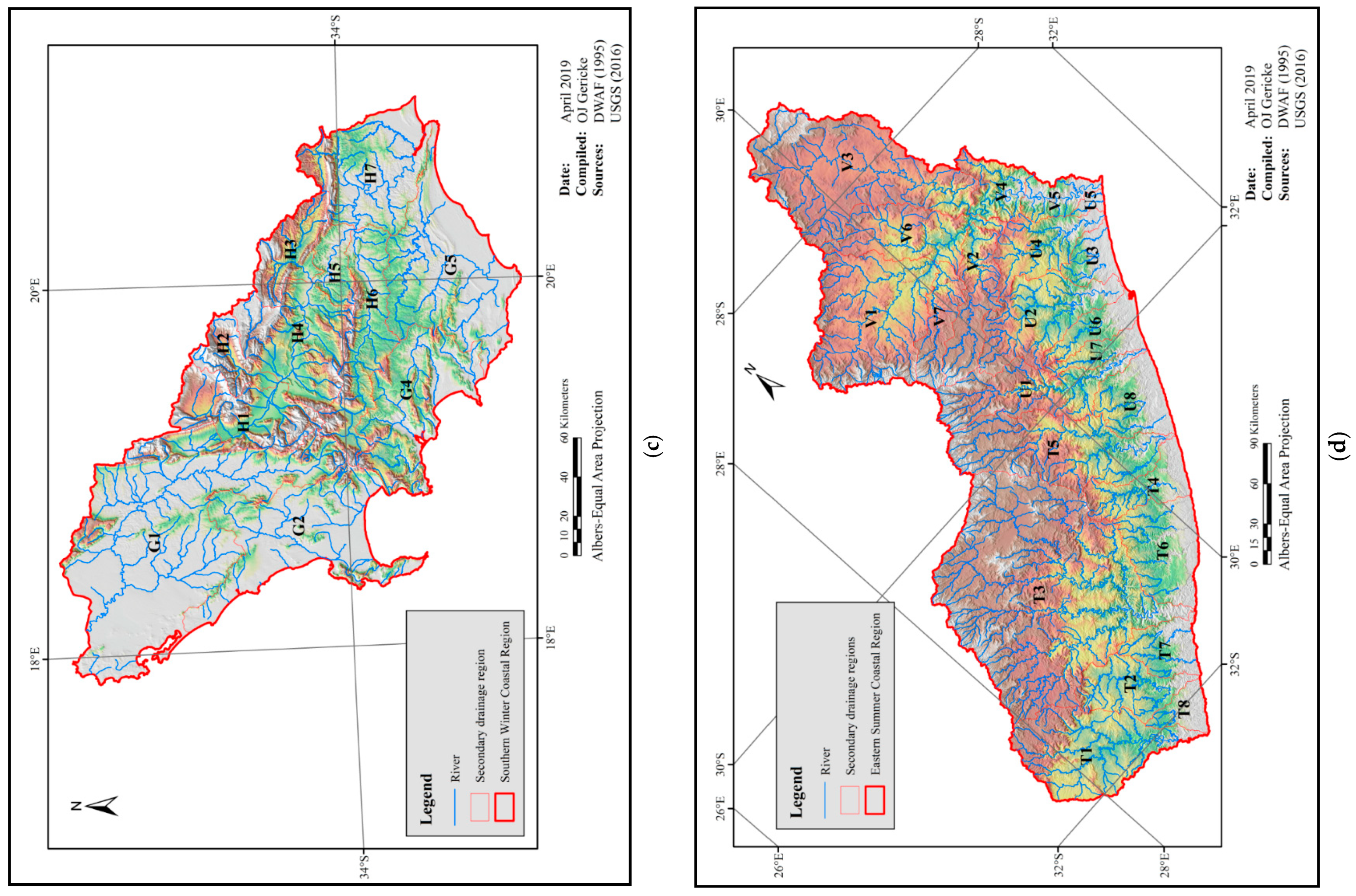
The 30-meter resolution DEMs and river network applicable to the four climatological regions are shown in Figure 2a–d.

The hydrologically corrected DEMs (cf. Figure 2a–d) provided accurate raster information to estimate the catchment area and all the other catchment characteristics as listed in Table A1, Table A2, Table A3 and Table A4 in Appendix A. It is also evident from these tables that catchment area influences both the volume of runoff and catchment response time, i.e., an increase in catchment area is associated with increases in both the volume of runoff and response time.

Catchment shape also proved to have an influence on both the catchment response time and runoff generation at a catchment level. In general, the wide, fan-shaped catchments characterized by lower shape factors (F_S, Equation (1)) and L_C:L_H ratios < 0.5, combined with steeper upper catchment slopes and flatter valleys, were characterized by shorter catchment response times and higher peak flows compared to those from the long, narrow, similar-sized catchments defined by larger F_S factors. The centroid distance (L_C) values listed in Table A1, Table A2, Table A3 and Table A4 in Appendix A not only confirm that L_C is influenced by the size and shape of a catchment, but also that L_C is influenced by the average catchment slope, especially in catchments with heterogeneous upper and lower catchment slope distributions. The average L_C:L_H ratio of 0.48 obtained confirms that the recommended L_C:L_H ratio of between 0.4 and 0.6 times the distance along the main river [7,42] is sufficiently accurate to be used in the various event-based design flood estimation methods. This is also a more definite guideline than the eyeball estimate as proposed by Alexander [6]. However, practitioners must assess each catchment individually using the tools available in ArcGIS^TM, before just using the proposed L_C:L_H ratios. For example, in many of the SWCR catchments (e.g., G1H008, H2H003, H4H006 and H6H003; Table A3) and ESCR catchments (e.g., T3H002, T5H004 and V6H002; Table A4), due to the steeper average catchment slopes (S₂, Equation (5)) between 14 and 37%, combined with heterogeneous catchment slopes, i.e., large differences between the average catchment slope and main river slopes (S₂:S_CH2 ratios > 25), the L_C:L_H ratios were much lower and varied between 0.21 and 0.38. In addition, it could also be argued that the extensive meandering of the main rivers in the SWCR and ESCR catchments also contributed to larger L_H values, hence, the lower L_C:L_H ratios observed.

In using Equation (2), completely circular catchments are defined by R_C ratios = 1. As shown in Table A1, Table A2, Table A3 and Table A4 in Appendix A, the R_C ratios varied between 1.26 and 2.10 at a catchment level in the four regions. In some of the partially ‘circular catchments’ (1 ≤ R_C < 1.5) with a homogeneous slope distribution in the NR and CR, the runoff from various parts in a catchment tend to reach the catchment outlet simultaneously. The catchments in the CR, and to a lesser extent the NR catchments, are also generally flatter with some surface depressions; hence, the longer catchment response times and lower peaks.

In different catchment area (A) ranges, the catchment response time from similar-sized elliptical catchments differed from those times witnessed in circular catchments with R_C ratios between 1 and 1.5. In elliptical catchments defined by R_C ratios > 1.5 and elongation ratios (R_E, Equation (3)) less than 0.45, the runoff proved to be more distributed over time, thus resulting in longer catchment response times. Examples thereof, as extracted from Table A1, Table A2, Table A3 and Table A4 in Appendix A, are listed in

Table 2. Examples of the impact that catchment shape, circularity, and elongation have on catchment response time in different area ranges.

Area Range (km2)	Catchment	A (km2)	FS (Equation (1))	RC (Equation (2))	RE (Equation (3))	TPx (Equation (9), h)
300 ≤ A < 600	U2H006	338	8.22	1.66	0.42	35.7
	G1H008	394	4.49	1.32	0.87	10.8
1000 ≤ A < 3000	V2H001	1951	18.39	1.73	0.26	47.1
	C5H012	2366	11.98	1.34	0.63	11.9
A > 20,000	V5H002	28,893	35.35	1.82	0.38	65.3
	C5H014	31,283	28.12	1.48	0.61	56.6

.

The average catchment slope results estimated using the Empirical method (Equation (4)) and Average Maximum Technique (Equation (5)) applicable to each catchment are listed in Table A1, Table A2, Table A3 and Table A4 in Appendix A and a scatter plot is shown in Figure 3.

Equation (5), as applied to the DEMs, was regarded as the most accurate method; hence, it was used as the baseline in the analysis. As shown in Figure 3, the r² value of 0.99 confirms the high degree of association between the results estimated using Equations (4) and (5). The Empirical method’s (Equation (4)) relatively low positive y-intercept value (0.41) and a slope value (1.18) that is larger than unity highlight that this method, despite being based on GIS-based input, has an overall tendency to overestimate the average catchment slope. On average, Equation (4) overestimated the average catchment slope with 18% in all the catchments under consideration when compared to Equation (5). In contrast, Gericke and Du Plessis [7] demonstrated that Equation (4) tends to underestimate the average catchment slopes with between 9 and 43% when compared to Equation (5) applied to the 90-m SRTM DEM data set. However, the latter results were only based on six mutually considered catchments, namely, C5H003, C5H012, 15, 16, 18 and C5H054, located in the Central Region. Differences of up to 46% are evident when the results based on the two versions of Equation (5), i.e., the 30-m (this study) versus 90-m [7] resolutions, are compared, while the two versions of Equation (4) only differ by up to 6%. The latter lower difference of only 6% could be ascribed to the fact that the 90-m and 30-m DEMs are well aligned in terms of horizontal offset; hence, resulting in a comparable catchment area (A) and length, e.g., contour length (M) computations. Hence, in considering the individual M:A ratios (expressed in km·km⁻²), it is evident that there is a direct relationship between the M:A ratios and average catchment slopes steeper than 3%, since steeper slopes will result in a higher contour density and associated M values. In considering the reclassified slope raster classes, it was evident that the prediction accuracy of the Empirical method increases with higher M:A ratios, i.e., the average percentage differences between Equations (4) and (5) are less significant. For example, 30% difference (slope class 0–3%), 23% difference (slope class 3–10%), 22% difference (slope class 10–30%), and 19% difference for average catchment slopes > 30%.

4.2. Channel Geomorphology

The average main river slopes estimated using Equations (6) to (8) are listed in Table A1, Table A2, Table A3 and Table A4 in Appendix A and a scatter plot is shown in Figure 4. Overall, the degree of association between these three methods is high, with the coefficient of determination (r² values) varying between 0.85 and 0.97. In South Africa, preference is given to the 10-85 method [41], since practitioners regard the Equal-area method largely as a graphical procedure, while the Taylor-Schwarz method is not widely used in South Africa [7]. However, the DWS locally [42] and the National Environmental Research Council internationally [45] recommend the use of the Taylor-Schwarz method (Equation (8)).

Catchment and river slopes have an influence on the catchment response time, which in turn impacts on the temporal distribution of rainfall and runoff processes. The correlation between the average catchment slopes (S₂, Equation (5)) and main river slopes (S_CH2, Equation (7)) is similar in the NR and CR, i.e., the average ratios of the slope descriptors (S₂:S_CH2) vary between 12 and 15. However, in the SWCR and ESCR, the average S₂:S_CH2 ratios are almost double that, with the average S₂:S_CH2 ratios equal to 27 and 32, respectively.

Such differences by a factor of 2 or more not only highlight the heterogeneous nature of the slope distributions in these catchments, but the impact of slope on catchment response time as well. Typically, in catchments characterized by high S₂:S_CH2 ratios (> 25) and low L_C:L_H ratios (< 0.4), the overall catchment response time proved to be shorter. In other words, runoff volumes reach and concentrate at the catchment centroid much quicker (due to the steeper catchment slope in the upper reaches), and in conjunction with the shorter L_C distances to follow to the catchment outlet, the resulting response time is shorter. Such results are typically evident in catchments H4H006 (S₂:S_CH2 = 63, L_C:L_H = 0.25) and T3H002 (S₂:S_CH2 = 106, L_C:L_H = 0.21).

The drainage density (D_D), expressed as the ratio of the total length of rivers within a catchment to the catchment area, determines the distance water travels down catchment slopes before reaching the main river reach and is therefore regarded as a key indicator of catchment response time and the resulting runoff due to the differences in velocity and residence time of water between the hill slopes and main rivers. As shown in Table A1, Table A3 and Table A4 in Appendix A, in the well-drained (D_D ≈ 0.3) catchments, e.g., A9H002 (NR), H1H018 (SWCR) and U2H006 (ESCR), more rainfall contributed effectively to direct runoff, while the response times were relatively shorter. All the catchments in the NR and CR, with the exception of A2H007 and C5H003, respectively, are characterized by a relatively low drainage density (D_D ≤ 0.20), hence, the longer catchment response times and lower peak flows (cf. Table A1 and Table A2).

4.3. Catchment Variables

The results for the different catchment variables expressed using CN values are listed in Table A1, Table A2, Table A3 and Table A4 in Appendix A. At a catchment level, the nature and spatial distribution of main land-use groups affected the temporal and spatial distribution of runoff. Overall, 90% of the catchments under consideration are classified as ‘rural pervious to semi-pervious catchments’ with more than 90% of the individual catchment areas underlain by hydrological soil groups B and C with a final infiltration capacity of between 6 and 13 mm·h⁻¹.

Urban areas only exceed 10% of the total catchment area in catchments A2H007 (36%), A2H019 (19%), C5H006 (13%), C5H054 (12%), H6H003 (14%) and U2H011 (22%). Hence, the impact of such low percentages of urbanization could be regarded as insignificant in this study, especially in catchments A2H007 and A2H019 where the high percentage of underlying dolomite (20–30%) will have neutralized the impact of the relatively higher percentages of urbanization present. In general, the local geology, i.e., underlying limestone and dolomite present in most of the NR catchments (cf. Table A1, Appendix A) contributed to the lower volume of direct runoff and peak flows in catchments A2H005, A2H012 and A3H001.

The influence of natural vegetation on runoff processes depends on the climatological region in which a particular catchment is situated, as well as the rainfall distribution. For example, the changes in seasonal and/or annual vegetal cover in the NR and CR introduced more variability in the runoff processes than in the SWCR and ESCR where the vegetal cover does not vary significantly between seasons. The weighted CN values (Table A1, Table A2, Table A3 and Table A4, Appendix A) varied between 59 and 77; these values clearly highlight the heterogeneous nature of the various catchment variables. Typically, higher CN values are associated with larger contributions to direct runoff and peak flow.

4.4. Conceptual Catchment Response Time Framework

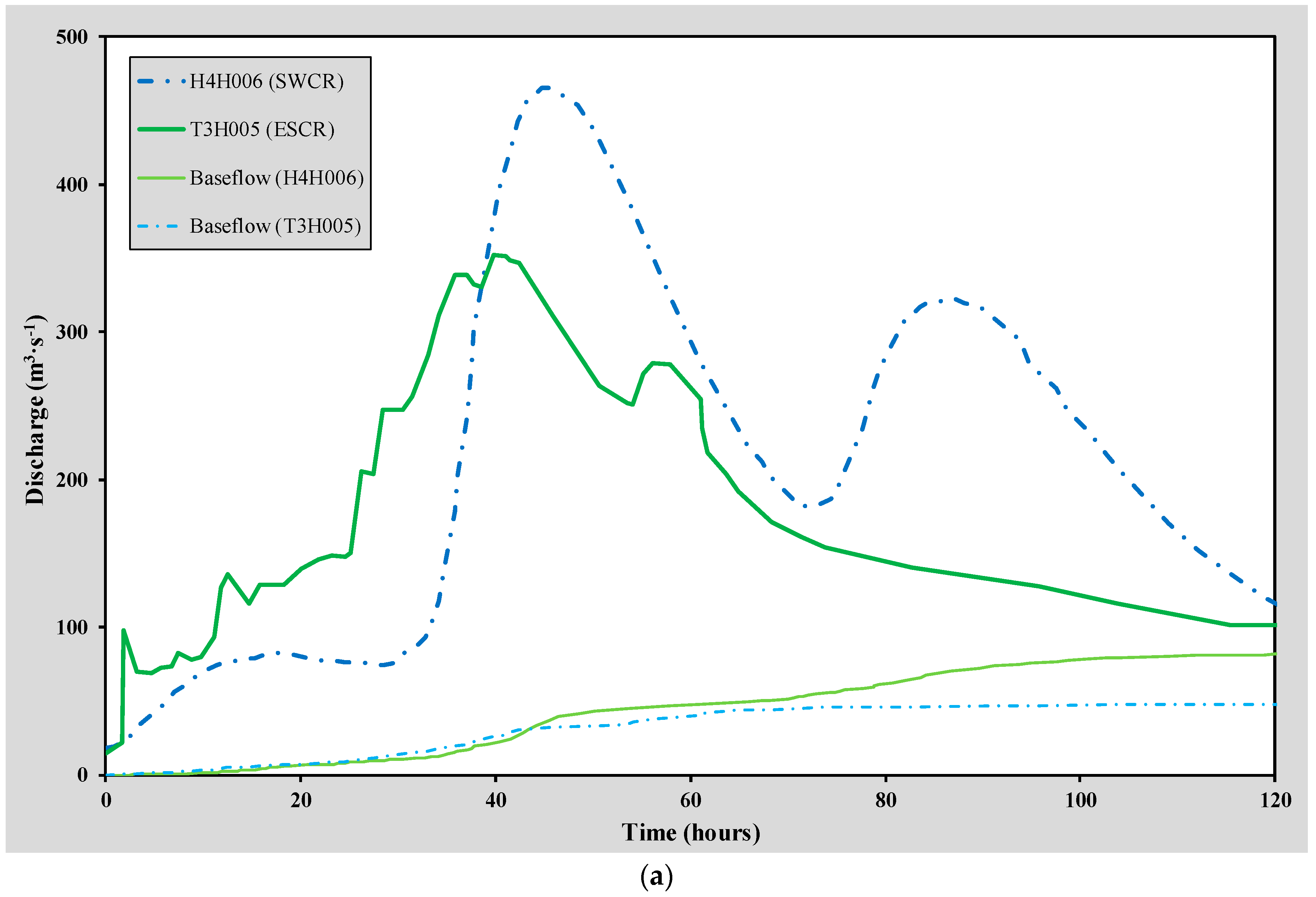
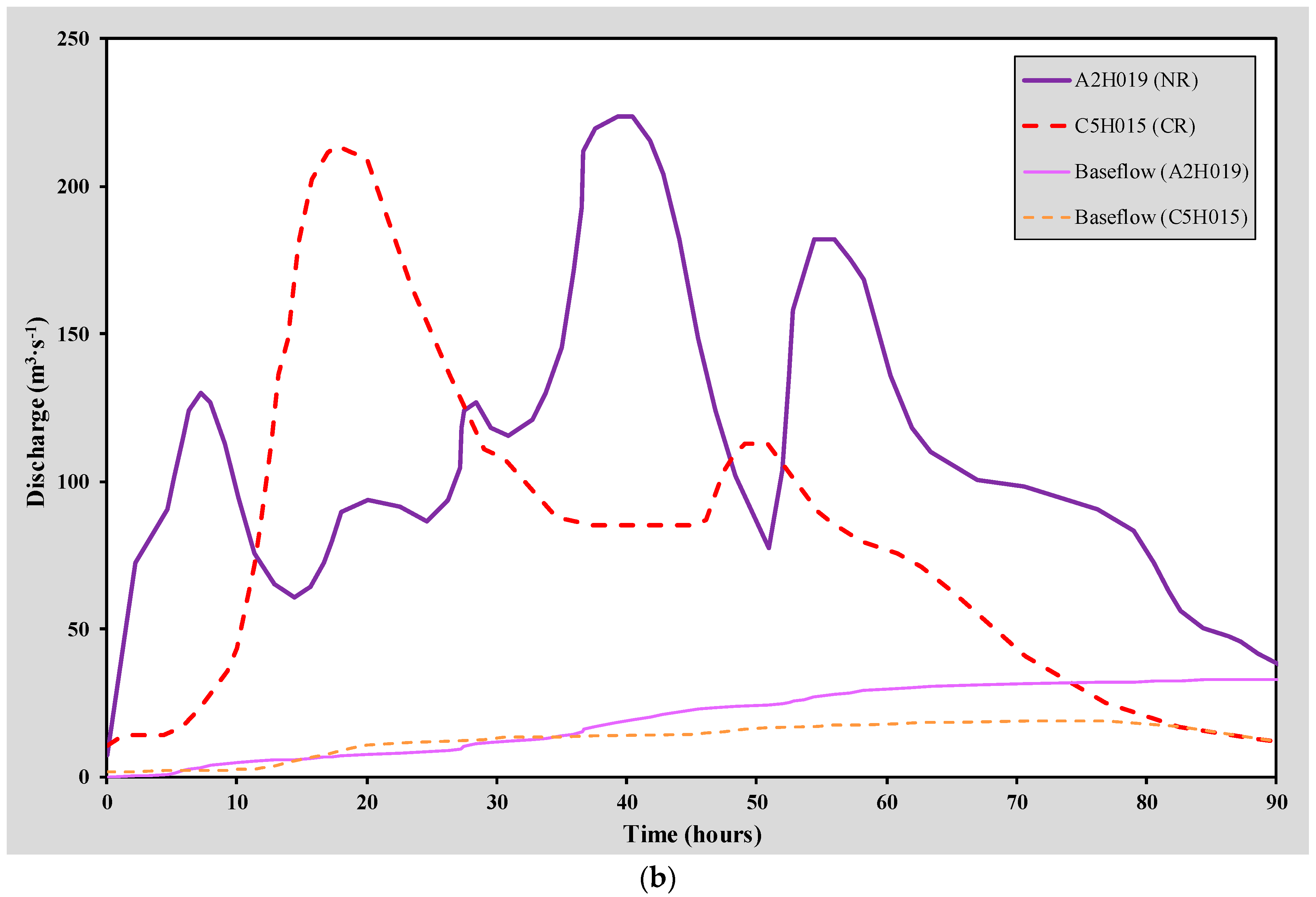
In order to elaborate on above discussion related to the combination of geomorphological catchment characteristics and the influence thereof on catchment response time, examples of hydrographs representative of the ‘average conditions’ (cf. Table A1, Table A2, Table A3 and Table A4, Appendix A) at a catchment level in two distinctive area ranges (e.g., A < 200 km² and 2500 km² ≤ A < 6500 km²) in each climatological region are presented in Figure 5 and Figure 6a,b, respectively.

The catchment areas which contributed to the resulting hydrographs shown in Figure 5 are comparable in size and range between 176 and 186 km²; hence, any differences in the catchment response and runoff generation in these catchments are not directly linked to catchment area intrinsically, but are more likely due to the heterogeneity of a combination of other geomorphological catchment characteristics.

In terms of shape, catchment U2H011 is regarded as the most elongated catchment characterized by the highest F_S factor (6.95) and lowest R_E ratio (0.42), while catchment A6H006 is regarded as the most fan-shaped catchment with the lowest F_S factor (5.16) and highest R_E ratio (0.60), respectively. Catchments C5H023 and G1H002 are very similar in terms of shape and elongation, while the circularity ratios (R_C) of all four catchments are similar and range between 1.3 and 1.4. Thus, based on shape alone, the catchment response time is expected to be the highest in catchment U2H011, followed by catchments C5H023, G1H002 and A6H006. However, this is not the case and it is clearly evident that the influence of shape on catchment response time in these catchments is overruled by the average catchment and river slopes. Typically, the much steeper average catchment and river slopes in catchments U2H011 (S₂ = 14.6% and S_CH2 = 1.3%) and G1H002 (S₂ = 33.5% and S_CH2 = 4.5%), resulted in shorter catchment response times, i.e., T_Pxi = 8.4 h and 6.0 h, respectively, as shown in Figure 5, while the peak flows (Q_Pxi) are about five-fold higher than in catchments A6H006 and C5H023.

As highlighted in the Introduction, Klein [29] regarded 300 km² as the upper area limit for ‘small’ catchments and claimed that the more rapid catchment response times are due to overland flow conditions being dominant. However, based on the results shown in Figure 5 and the discussion above, it is obvious that catchment response time could not be limited and specifically assigned to pre-defined catchment area ranges (A ≤ 300 km²) and specific flow regimes without considering the combined influence of different geomorphological catchment characteristics on response time and runoff generation. Hydrological literature (e.g., [46,47,48]) also highlighted that overland flow conditions are limited to the upper reaches of a catchment and depends on the slope and surface roughness.

In contrast to the single-peaked hydrographs associated with ‘small’ catchments as illustrated in Figure 5, the multi-peaked hydrographs shown in Figure 6a,b are due to an increasing heterogeneity of geomorphological catchment characteristics and the spatial–temporal rainfall distribution as the catchment scale increases.

The association as established in the ‘small’ catchments between high F_S factors, low R_E ratios and/or flatter slope (S₂ and S_CH2) values resulting in longer catchment response times, larger direct runoff volumes and lower peaks, was not that prominent in the ‘medium to large’ catchments. However, the lower drainage densities (D_D ≤ 0.20) and differences in catchment size (e.g., A2H019 = 6120 km²; C5H015 = 5939 km²; H4H006 = 2878 km² and T3H005 = 2565 km²) are more significant than the combined influence of the afore-mentioned catchment characteristics.

Ultimately, it could be argued that the type, spatial and temporal distribution of rainfall govern the overall catchment response time at medium to large catchment scales, as illustrated in Figure 6a,b, respectively. However, the spatial and temporal distribution of rainfall are not regarded as ‘geomorphological catchment characteristics’ and hence, the quantitative investigation thereof is beyond the scope of this study. However, in terms of rainfall type and spatial distribution, the convective summer rainfall events in the semi-arid catchments A2H019 (NR) and C5H015 (CR) will typically be more non-uniform with an intermittent spatial distribution compared to the orographic or frontal winter rainfall in catchment H4H006 (SWCR) and the all-year rainfall in catchment T3H005 (ESCR), respectively. Although not being analyzed quantitatively, such general conclusions could be drawn from Figure 6a,b based on the differences evident in the hydrograph shape, i.e., the shorter catchment response times (T_Pxi < 25 h), lower direct runoff volumes (Q_Dxi ≤ 30 × 10⁶ m³) and well-defined peaks (Q_Pxi ≤ 215 m³·s⁻¹) associated with much larger catchment areas (A > 5900 km²) in the case of catchments A2H019 and C5H015 (Figure 6b) as opposed to the much larger direct runoff volumes (Q_Dxi ≈ 74 × 10⁶ m³) and peak flows (Q_Pxi > 350 m³·s⁻¹) associated with smaller catchment areas less than 2900 km² in the case of catchments H4H006 and T3H005 (cf. Figure 6a).

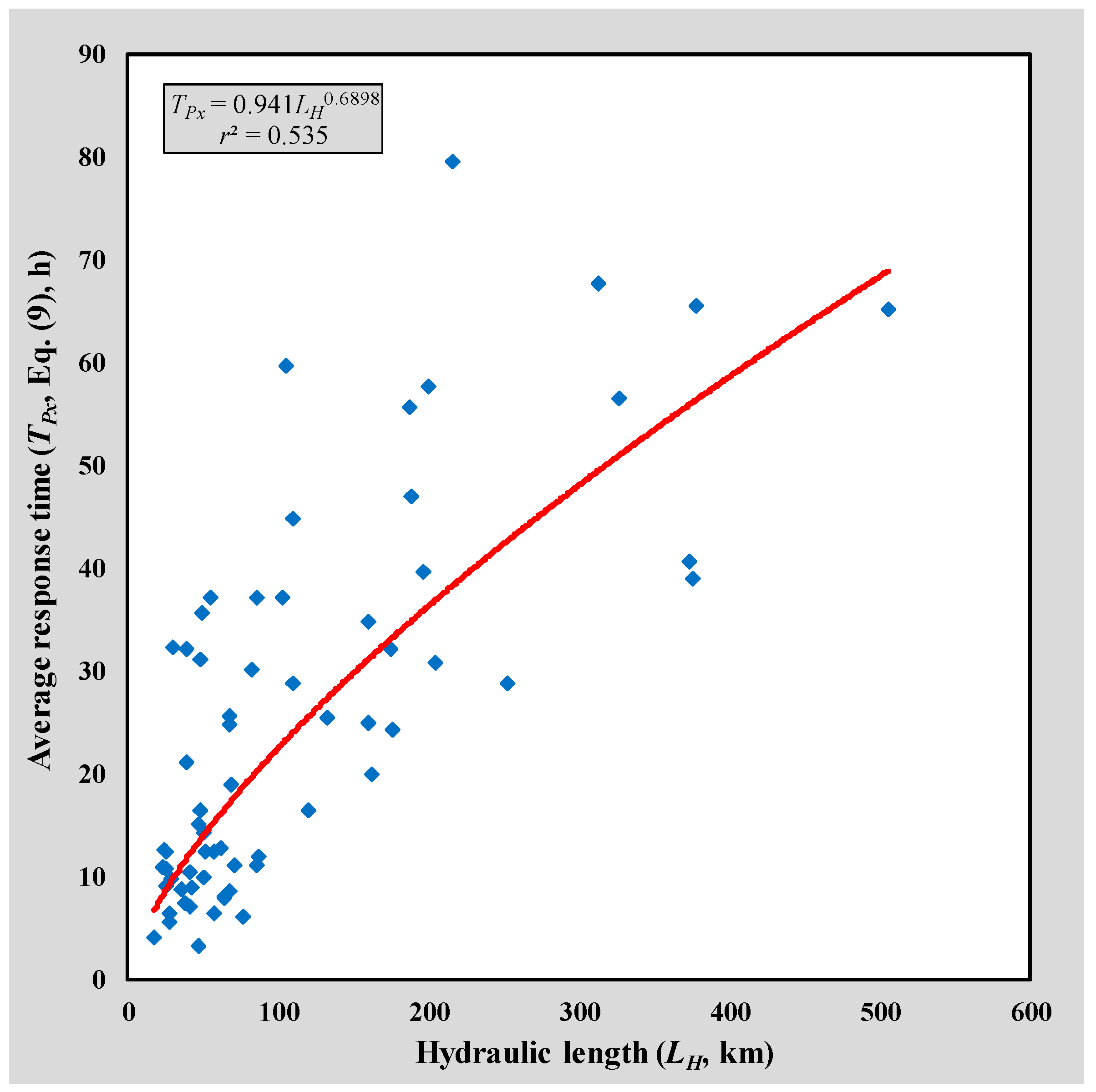
In estimating the average catchment response time (T_Px values; Equation (9)), least square regression analyses in a power form (y = ax^b) yielded the highest r² values in all cases when the various independent predictor variables, i.e., geomorphological catchment characteristics, were included as part of a conceptual catchment response time framework. Only the six geomorphological catchment characteristics demonstrating a moderate degree of association (r² value ≥ 0.4) with the observed T_Px values are included in

Table 3. Correlation matrix between the observed time to peak values (T_Px; Equation (9)) and geomorphological catchment characteristics.

Parameter	TPx (h)	A (km2)	P (km)	LH (km)	LC (km)	FS (Equation (1))	S2:SCH2 Ratio
TPx (h)	1.00	-	-	-	-	-	-
A (km2)	0.41	1.00	-	-	-	-	-
P (km)	0.43	0.99	1.00	-	-	-	-
LH (km)	0.54	0.89	0.91	1.00	-	-	-
LC (km)	0.47	0.82	0.84	0.93	1.00	-	-
FS (Equation (1))	0.51	0.87	0.89	0.98	0.98	1.00	-
S2:SCH2 Ratio	0.48	0.18	0.19	0.27	0.21	0.25	1.00

. A correlation matrix is used to highlight the various relationships.

It is evident from Table 3 and Figure 7 that L_H is the single best independent predictor variable of T_Px in all the catchments, with r² = 0.54. However, all the other independent predictor variables could be regarded as equally important, hence, confirming that distinct relationships are not always apparent when individual geomorphological catchment characteristics are considered in isolation to represent the complexities of catchment response time.

The final derived regression applicable to all the catchments is shown in Equation (10):

$$T_{Py}=1.018A^{0.327}-0.149P^{0.659}-2.089{\left(L_H{L}_C\right)}^{0.300}-0.281\left(\frac{S_2}{S_{CH2}}\right),$$

(10)

where T_Py is the estimated time to peak (h), A is the catchment area (km²), L_C is the centroid distance (km), L_H is the hydraulic length (km), P is the catchment perimeter (km), S₂ is the average catchment slope (Equation (5), %), and S_CH2 is the average river slope (Equation (7), %).

In comparing the estimated T_Py (Equation (10)) with the observed T_Px (Equation (9)) values, an improved coefficient of multiple-correlation (R_i²) = 0.62 and standard error (S_Ey) = 11.9 h were obtained. However, the S_Ey results must be clearly understood in the context of the actual response time associated with catchment area, as the impact of such error in the T_Py estimates might be critical in a small catchment, while being less significant in a larger catchment.

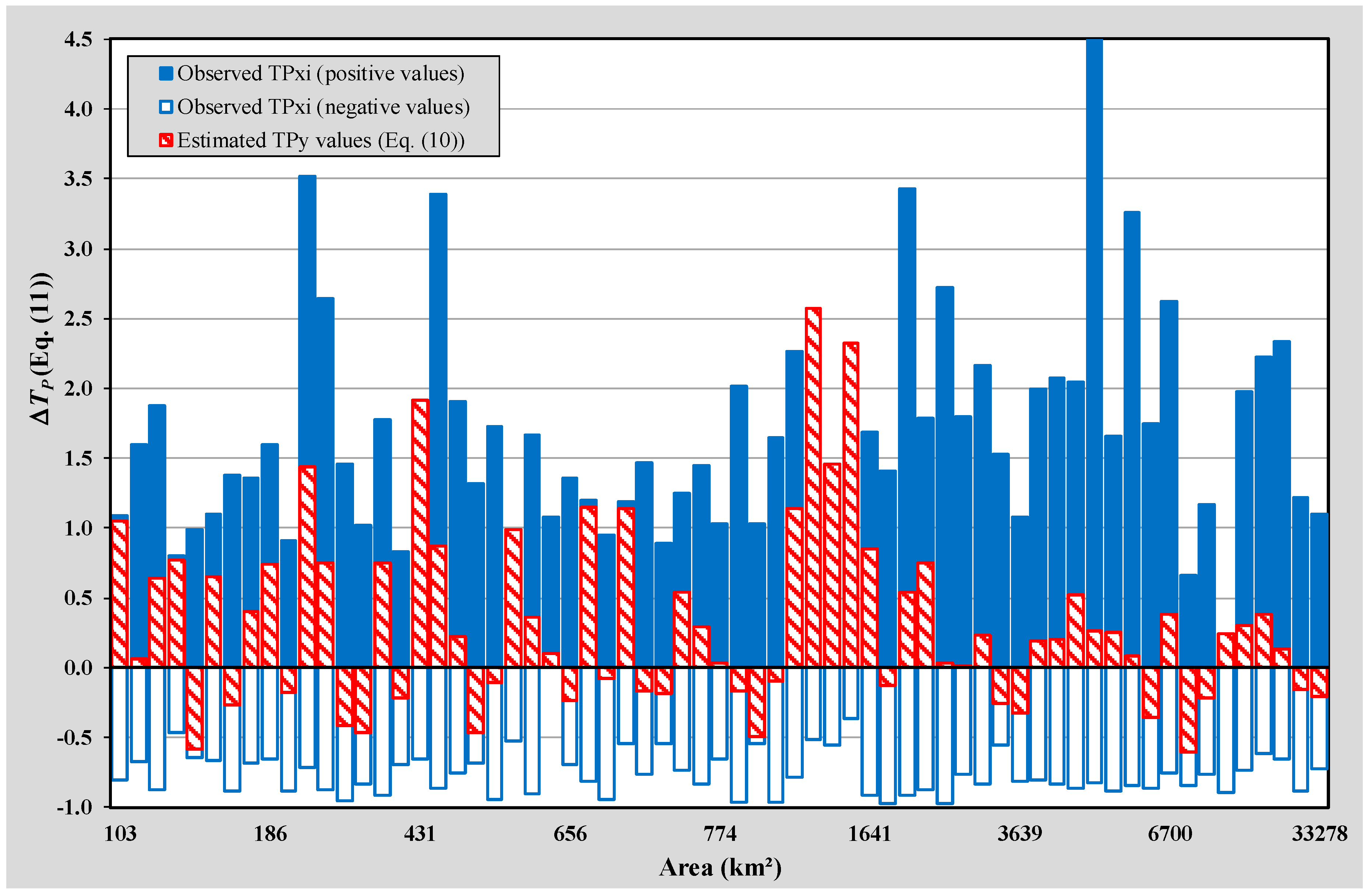
The high variability of individual-event observed T_Pxi and estimated T_Py (Equation (10)) values relative to the average observed catchment T_Px values (Equation (9)) in each catchment is estimated using Equation (11). The latter catchment response time variability at a catchment level in the four climatological regions are shown in Figure 8.

$$\Delta T_P=\left(\frac{T_{Pxi},T_{Py}}{T_{Px}}\right)-1,$$

(11)

where ΔT_P is the catchment response time variability (positive = overestimation and negative = underestimation), T_Px is the average observed catchment response time (Equation (9), h), T_Pxi is the individual-event observed catchment response time expressed as the net duration of a multi-peaked hydrograph (h), and T_Py is the estimated catchment response time (Equation (10), h).

The high T_Pxi variability, as depicted in Figure 8 and expressed using Equation (11), highlights that the variability in observed catchment response times is not solely related to catchment area, but the increase in variability is most likely associated with an increase in the spatial and temporal distribution and heterogeneity of other geomorphological catchment characteristics and rainfall as the catchment scale increases. Typically, at these catchment scales, the largest Q_Pxi and T_Pxi values are associated with the likelihood of the entire catchment receiving rainfall for the critical storm duration. Smaller T_Pxi values could be expected when effective rainfall of high average intensity does not cover the entire catchment, especially when a rainfall event is centered near the catchment outlet. However, these smaller T_Pxi values are likely to occur more frequently; hence, having a larger influence on the average value and consequently might result in an underestimated representative catchment T_Px value. On the other hand, the longer T_Pxi values have a lower frequency of occurrence and are reasonable at medium to large catchment scales as the contribution of the whole catchment to peak discharge seldom occurs as a result of the non-uniform spatial and temporal distribution of rainfall. Ultimately, it can be concluded that catchment response time variability increases as the magnitude (e.g., AEP) and spatial distribution of rainfall events decrease.

Despite the moderate GOF results achieved in using Equation (10), it is clearly evident from Figure 8 that the T_Py estimates are well within the bounds of the high individual-event observed T_Pxi variability in each catchment. However, since the purpose of this study is not to derive an empirical catchment response time equation, the further refinement of Equation (10) in terms of calibration, verification and possible regionalization is acknowledged. Equation (10) was purposely derived to illustrate that the response of a catchment is most likely to be influenced by a combination of geomorphological catchment characteristics and not by a single catchment characteristic. Furthermore, as in agreement with the findings of [25], the inclusion of slope predictors (S₂ and S_CH2) is regarded as essential to ensure that both the size (A) and distance (L_C and L_H) predictors provide a good indication of catchment response times. The distance predictors, in conjunction with the catchment perimeter (P), also proved to be useful in describing the catchment shape when used in combination with the catchment area.

5. Conclusions

The use of specialized GIS spatial modelling tools and conventional equations in conjunction with standard GIS tools resulted in comprehensive and comparable catchment parameter estimations, which ultimately contributed towards the better understanding of the linkage between geomorphological catchment characteristics and response time. The advantages of using such GIS-based approach could be summarized as follows:

• A more diverse selection of catchment parameters could be considered as opposed to when manual methods are used and were included as independent predictor variables in the conceptual catchment response time framework to evaluate the individual and combined influences of catchment geomorphology, channel geomorphology and catchment variables on response time and runoff generation.
• The inherent human and instrumentation errors associated with manual data acquisition processes are eliminated. However, the original meta data used in any GIS-based approach must always be obtained from reputable data custodians and/or repositories.
• The time and effort to extract information manually not only limit the number of catchment parameters being considered by researchers when undertaking multiple regression analysis and regionalization procedures, but also lead to systematic errors and inconsistent methodologies, which are not necessarily well documented and/or recognized by the broader scientific community. In using a GIS-based approach, a trade-off between time and accuracy could be used to provide results at a pre-defined or required resolution and accuracy.

In terms of catchment geomorphology, the hydrologically corrected DEMs at a 30-m resolution provided accurate raster information to estimate the catchment areas and all the other relevant catchment characteristics. It was also evident that the 30-m (this study) and 90-m [7] DEMs are well aligned and without any significant horizontal offset; hence, the area and length computations using both the datasets have identical values. However, vertical accuracy, as shown by the comparisons between Equations (4) and (5), decreases with an increase in slope and elevation due to the possible presence of large outliers and sinks. The use of the Average Maximum Technique (Equation (5)), as applied to the DEMs, is regarded as the most accurate method to estimate the average catchment slope, although, the application of the Empirical method (Equation (4)), in conjunction with standard GIS tools, proved to be equally accurate and it is also very useful for the identification of slope frequency distribution classes. In terms of channel geomorphology, the use of the Longest Flow Path tool in the Hydrology toolset is recommended to estimate the length of main rivers, while the Stack Profile tool proved to be very efficient in generating longitudinal river profiles from DEM data. The high degree of association (0.85 ≤ r² ≤ 0.97) between the various methods (Equations (6)–(8)) used to estimate the average main river slopes confirmed that any of these methods could be used with confidence. However, preference is given to the 10-85 method (Equation (7)), since it is more user friendly to use than the other two methods, while being equally accurate.

The high degree of association between the different GIS-based catchment parameter estimation methods not only confirmed that the comprehensive set of spatial and hydrological tools available in ArcGIS^TM was successfully applied, but that any of these methods could also be used satisfactorily and with confidence in flood hydrology. Such improved estimations of geomorphological catchment characteristics are not only essential to both regionalization procedures and the actual estimation of design floods, but it will also impact on the successful deployment thereof. Hence, taking into consideration the significant influence catchment response times have on the resulting hydrograph shape and peak flow, it is obvious that the accuracy of these GIS-based catchment parameter estimation methods, irrespective of the software package used, will also have an indirect impact on the design of hydraulic structures.

In this paper, the individual and combined influences of various geomorphological catchment characteristics on response time and runoff generation were evaluated in different catchment area ranges. In general, catchment and channel geomorphology overruled the impact that catchment variables might have on the response time and resulting runoff. In considering catchment and channel geomorphology, shorter catchment response times and higher peak flows were evident in catchments of comparable size characterized by lower shape factors (F_S), L_C:L_H ratios (<0.5) and circularity ratios (1 ≤ R_C < 1.5), and associated higher elongation ratios (R_E > 0.5), S:S_CH ratios (>25) and drainage densities (D_D ≈ 0.3).

In catchment areas ≤ 200 km², the response time was primarily influenced and governed by the average catchment and river slopes, i.e., the S:S_CH ratios. In catchment areas between 2500 and 6500 km², no distinctive linkage was apparent between the observed catchment response time and catchment shape, average catchment and river slopes. At these catchment scales, the combined influence of the latter catchment parameters was less significant than the differences in catchment size and drainage densities. The type, spatial and temporal distribution of rainfall were identified as possible candidates that govern the overall catchment response time at medium to large catchment scales, but the quantitative investigation thereof is beyond the scope of this study and could therefore not be confirmed. However, it was also evident that catchment response time could not be limited and specifically assigned to pre-defined catchment area ranges and associated flow regimes without considering the combined influence of the above-mentioned geomorphological catchment characteristics and rainfall characteristics. In other words, the variability in observed catchment response times is not exclusively related to catchment area, but rather associated with the increasing spatial–temporal heterogeneity of other geomorphological catchment characteristics and rainfall as the catchment scale increases.

References

- Rao, A.R.; Srinivas, V.V. Some Problems in Regionalisation of Watersheds. In Water Resources Systems: Water Availability and Global Change, Proceedings of Symposium HS02a Held During IUGG 2003, the XXIII General Assembly of the International Union of Geodesy and Geophysics, Sapporo, Japan, 30 June–11 July 2003; Franks, S.W., Ed.; Publication No. 280; IAHS Publications: Wallingford, UK, 2003; pp. 301–308. [Google Scholar]
- Burn, D.H. Catchment similarity for regional flood frequency analysis using seasonality measures. J. Hydrol. 1997, 202, 212–230. [Google Scholar] [CrossRef]
- McCuen, R.H. Hydrologic Analysis and Design, 3rd ed.; Prentice-Hall: New York, NY, USA, 2005. [Google Scholar]
- Hosking, J.R.M.; Wallis, J.R. Regional Frequency Analysis: An Approach Based on L-Moments; Cambridge University Press: Cambridge, UK, 1997. [Google Scholar]
- Burn, D.H. Evaluation of regional flood frequency analysis with a region of influence approach. Water Resour. Res. 1990, 26, 2257–2265. [Google Scholar] [CrossRef]
- Alexander, W.J.R. Flood Risk Reduction Measures: Incorporating Flood Hydrology for Southern Africa; Department of Civil and Biosystems Engineering, University of Pretoria: Pretoria, Sounth Africa, 2001. [Google Scholar]
- Gericke, O.J.; Du Plessis, J.A. Catchment parameter analysis in flood hydrology using GIS applications. J. S. Afr. Inst. Civ. Eng. 2012, 54, 15–26. [Google Scholar]
- Cleveland, T.G.; Garcia, A.; He, X.; Fang, X.; Thompson, D.B. Comparison of Physical Characteristics for Selected Small Watersheds in Texas as determined by Automated and Manual methods. In Proceedings of the Texas ASCE Section Fall Meeting, El Paso, TX, USA, 24–26 January 2005. [Google Scholar]
- Fang, X.; Thompson, D.B.; Cleveland, T.G.; Pradhan, P.; Malla, R. Time of concentration estimated using watershed parameters by automated and manual methods. J. Irrig. Drain. Eng. 2008, 134, 202–211. [Google Scholar] [CrossRef]
- Keshtkaran, P.; Sabzevari, T. Prediction of geomorphologic parameters of catchment without GIS to estimate runoff using GIUH model. Hydrol. Earth Syst. Sci. Discuss. 2016. [Google Scholar] [CrossRef]
- Dongquan, Z.; Jining, C.; Haozheng, W.; Qingyuan, T.; Shangbing, C.; Zheng, S. GIS-based urban rainfall-runoff modelling using an automatic catchment discretization approach: A case study in Macau. Environ. Earth Sci. 2009, 59, 465–472. [Google Scholar] [CrossRef]
- El Bastawesy, M.; Faid, A.; El Gammal, E. The quaternary development of tributary channels to the Nile River at Kom Ombo area, Eastern Desert of Egypt, and their implication for groundwater resources. Hydrol. Process. 2010, 24, 1856–1865. [Google Scholar] [CrossRef]
- Rao, N.; Latha, S.; Kumar, A.; Krishna, H. Morphometric analysis of Gostani River Basin in Andhra Pradesh State, India using spatial information technology. Int. J. Geomat. Geosci. 2010, 1, 179–187. [Google Scholar]
- ESRI. ArcGIS 10.5 Desktop Help. Redlands, CA: Environmental Systems Research Institute. Available online: https://www.webhelp.esri.com/arcgisdesktop (accessed on 19 September 2016).
- GRASS. GRASS User’s Guide. Geographic Resources Analysis Support System, Open Source Geospatial Foundation. Available online: http://grass.osgeo.org (accessed on 26 July 2017).
- QGIS. QGIS User’s Guide. Quantum Geographical Information System, Open Source Geospatial Foundation. Available online: http://qgis.osgeo.org (accessed on 26 July 2017).
- Jena, S.K.; Tiwari, K.N. Modelling synthetic unit hydrograph parameters with geomorphological parameters of watersheds. J. Hydrol. 2006, 319, 1–14. [Google Scholar] [CrossRef]
- Rodríguez-Iturbe, I.; Valdés, J.B. The geomorphologic structure of hydrologic response. Water Resour. Res. 1979, 15, 1409–1420. [Google Scholar] [CrossRef] [Green Version]
- Beven, K.J.; Wood, E.F.; Sivapalan, M. On hydrological heterogeneity—Catchment geomorphology and catchment response. J. Hydrol. 1988, 100, 353–375. [Google Scholar] [CrossRef]
- Royappen, M.; Dye, P.J.; Schulze, R.E.; Gush, M.B. An Analysis of Catchment Attributes and Hydrological Response Characteristics in a Range of Small Catchments; WRC Report No. 1193/01/02; Water Research Commission: Pretoria, South Africa, 2002. [Google Scholar]
- Smithers, J.C. Review: Methods for design flood estimation in South Africa. Water SA 2012, 38, 633–646. [Google Scholar] [CrossRef]
- Alexander, W.J.R. The standard design flood. J. S. Afr. Inst. Civ. Eng. 2002, 44, 26–30. [Google Scholar]
- Bondelid, T.R.; McCuen, R.H.; Jackson, T.J. Sensitivity of SCS models to curve number variation. Water Resour. Bull. 1982, 20, 337–349. [Google Scholar] [CrossRef]
- Gericke, O.J.; Smithers, J.C. Review of methods used to estimate catchment response time for the purpose of peak discharge estimation. Hydrol. Sci. J. 2014, 59, 1935–1971. [Google Scholar] [CrossRef]
- Gericke, O.J.; Smithers, J.C. Derivation and verification of empirical catchment response time equations for medium to large catchments in South Africa. Hydrol. Process. 2016, 30, 4384–4404. [Google Scholar] [CrossRef]
- Heerdegen, R.G.; Reich, B.M. Unit hydrographs of catchments of different sizes and dissimilar regions. J. Hydrol. 1974, 22, 143–153. [Google Scholar] [CrossRef]
- Ward, R.C.; Robinson, M. Principles of Hydrology, 3rd ed.; McGraw-Hill: London, UK, 1999. [Google Scholar]
- Pegram, G.G.S.; Parak, M. A review of the Regional Maximum Flood and Rational formula using geomorphological information and observed floods. Water SA 2004, 30, 377–392. [Google Scholar] [CrossRef]
- Klein, M. Hydrograph peakedness and basin area. Earth Surf. Process. 1976, 1, 1–14. [Google Scholar] [CrossRef]
- Murphey, J.B.; Wallace, D.E.; Lane, L.J. Geomorphic parameters predict hydrograph characteristics in the southwest. Water Resour. Bull. 1977, 13, 25–38. [Google Scholar] [CrossRef]
- Cook, R.; Doornkamp, J. Geomorphology in Environmental Management, 2nd ed.; Oxford University Press: London, UK, 1990. [Google Scholar]
- Arnaud, P.; Bouvier, C.; Cisneros, L.; Dominguez, R. Influence of rainfall spatial variability on flood prediction. J. Hydrol. 2002, 260, 216–230. [Google Scholar] [CrossRef]
- Brath, A.; Montanari, A.; Toth, E. Analysis of the effects of different scenarios of historical data availability on the calibration of a spatially-distributed hydrological model. J. Hydrol. 2004, 291, 232–253. [Google Scholar] [CrossRef]
- Pechlivanidis, I.G.; McIntyre, N.; Wheater, H.S. The significance of spatial variability of rainfall on simulated runoff: An evaluation based on the Upper Lee catchment, UK. Hydrol. Res. 2017, 48, 1118–1130. [Google Scholar] [CrossRef]
- Schulze, R.E.; Schmidt, E.J.; Smithers, J.C. SCS-SA User Manual: PC-based SCS Design Flood Estimates for Small Catchments in Southern Africa; ACRU Report No. 40; Department of Agricultural Engineering, University of Natal: Pietermaritsburg, South Africa, 1992. [Google Scholar]
- Midgley, D.C.; Pitman, W.V.; Middleton, B.J. Surface Water Resources of South Africa; WRC Report No. 298/2/94; Water Research Commission: Pretoria, South Africa, 1994. [Google Scholar]
- Gericke, O.J.; Smithers, J.C. Direct estimation of catchment response time parameters in medium to large catchments using observed streamflow data. Hydrol. Process. 2017, 31, 1125–1143. [Google Scholar] [CrossRef]
- DWAF. GIS Data: Drainage Regions of South Africa; Department of Water Affairs and Forestry: Pretoria, South Africa, 1995.
- ESRI. ArcGIS Desktop Help: Map Projections and Coordinate Systems; Environmental Systems Research Institute: Redlands, CA, USA, 2006. [Google Scholar]
- USGS. EarthExplorer; United States Geological Survey. Available online: https://earthexplorer.usgs.gov/ (accessed on 19 September 2016).
- SANRAL. Drainage Manual, 6th ed.; South African National Roads Agency Limited: Pretoria, South Africa, 2013.
- Van der Spuy, D.; Rademeyer, P.F. Flood Frequency Estimation Methods as applied in the Department of Water Affairs; Department of Water and Sanitation: Pretoria, South Africa, 2018.
- CSIR. GIS Data: Classified Raster Data for National Coverage based on 31 Landcover Types; Council for Scientific and Industrial Research, Environmentek: Pretoria, South Africa, 2001. [Google Scholar]
- Nathan, R.J.; McMahon, T.A. Evaluation of automated techniques for baseflow and recession analyses. Water Resour. Res. 1990, 26, 1465–1473. [Google Scholar] [CrossRef]
- NERC. Flood Studies Report; Natural Environment Research Council: London, UK, 1975. [Google Scholar]
- Viessman, W.; Lewis, G.L. Introduction to Hydrology, 4th ed.; Harper Collins College Publishers Incorporated: New York, NY, USA, 1996. [Google Scholar]
- Seybert, T.A. Stormwater Management for Land Development: Methods and Calculations for Quantity Control; John Wiley and Sons Incorporated: Hoboken, NJ, USA, 2006. [Google Scholar]
- USDA NRCS. Time of concentration. In National Engineering Handbook; Woodward, D.E., Hoeft, C.C., Humpal, A., Cerrelli, G., Eds.; Chapter 15, Section 4, Part 630; United States Department of Agriculture Natural Resources Conservation Service: Washington, DC, USA, 2010; pp. 1–18. [Google Scholar]
Figure 2.
(a) Digital Elevation Model (DEM) of the Northern Region. The altitude above mean sea level (MSL) varies between 544 and 2089 m. The river network shown is characterized by drainage densities (DD) at a catchment level ranging between 0.09 and 0.24. (b) DEM of the Central Region. The altitude above MSL varies between 993 and 2130 m. The river network shown is characterized by drainage densities (DD) at a catchment level ranging between 0.11 and 0.23. (c) DEM of the Southern Winter Coastal Region. The altitude above MSL varies between 0 and 2235 m. The river network shown is characterized by drainage densities (DD) at a catchment level ranging between 0.17 and 0.28. (d) DEM of the Eastern Summer Coastal Region. The altitude above MSL varies between 0 and 3420 m. The river network shown is characterized by drainage densities (DD) at a catchment level ranging between 0.14 and 0.30.
Figure 3.
Scatter plot of the average catchment slope values estimated using Equations (4) and (5).
Figure 4.
Scatter plot of the average river slope values estimated using Equations (6)–(8). The degree of association (r2 values) between the different methods range between 0.85 (Equation (7) vs. Equation (8)) and 0.97 (Equation (6) vs. Equation (7)).
Figure 5.
Examples of observed hydrographs representative of the ‘average conditions’ in ‘small’ catchments (100 km2 ≤ A < 200 km2) in each climatological region.
Figure 6.
(a) Examples of observed hydrographs representative of the ‘average conditions’ in ‘medium’ catchments (2500 km2 ≤ A < 3000 km2) in the SWCR and ESCR. (b) Examples of observed hydrographs representative of the ‘average conditions’ in ‘large’ catchments (5500 km2 ≤ A < 6500 km2) in the NR and CR.
Figure 7.
Relationship between the average catchment response time (Equation (9)) as the criterion variable and the hydraulic length (LH) as the predictor variable in the 65 catchments.
Figure 8.
Catchment response time variability (Equation (11)) at a catchment level in the four climatological regions.