Attributing Changes in Streamflow to Land Use and Climate Change for 472 Catchments in Australia and the United States


1
Water Engineering and Management Group, Faculty of Engineering Technology, University of Twente, 7500 AE Enschede, The Netherlands
2
Faculty of Forestry, Universitas Gadjah Mada, Yogyakarta 55281, Indonesia
*
Author to whom correspondence should be addressed.
Water 2019, 11(5), 1059; https://doi.org/10.3390/w11051059
Submission received: 4 April 2019
/
Revised: 7 May 2019
/
Accepted: 16 May 2019
/
Published: 21 May 2019
(This article belongs to the Special Issue Hydrological Processes under Environmental Change)
Abstract
:A data-based method to distinguish climate and land use change impacts on streamflow has been previously developed and needs further evaluation through a large sample study. This study aims to apply the method to a large sample set of 472 catchments in the United States and Australia. The method calculates the water and energy budget of a catchment which can be translated to climate and land use induced changes in streamflow between two periods: a pre-change and post-change period. Several geographical characteristics (e.g., aridity index, average catchment slope, historical land use) were considered for the interpretation of the results. The results show that in general as expected, an increase of the annual discharge is caused by deforestation and a wetter climate, and a decrease of the annual discharge is caused by afforestation and a drier climate. In addition, changes in streamflow of American catchments are likely caused by a wetter climate, while changes in streamflow of Australian catchments are caused by a wetter or drier climate. It can be concluded that the method performs reasonably well and that the results are best explained by the location of the catchment, the aridity index and historical land use.
Keywords:
climate change; land use change; discharge; attribution; data-based; Australia; United States1. Introduction
Climate change and land use change affect the hydrological regime by changing the rainfall partitioning into actual evapotranspiration and runoff. Changes in rainfall intensity and extremes have been found in numerous studies, which often indicated tendencies towards higher frequencies of rainfall extremes (e.g., [1,2,3,4,5]). These changes are relevant for instance to water resources management, agriculture and forestry. Climate and land-use changes operate at different temporal and spatial scales and can act simultaneously enhancing or weakening their effects [6,7,8]. Hence, the attribution of observed hydrological changes to climate change and/or land use change can be highly uncertain [9]. The attribution of hydrological changes, such as alterations in streamflow, is important to understand effects of climate and land-use changes in the past and to estimate effects of climate and land-use changes in the future. This attribution is relevant for water management of catchments, because it separates the causes of hydrological changes enabling more focused approaches to mitigate and adapt to impacts of future changes. A large sample study will provide more insight in the attribution of streamflow changes and the potential and limitations of the attribution method.
Attribution methods can be divided into modelling and non-modelling approaches. An advantage of modelling approaches is that the outcome generally is more reliable, however, the applicability of the approaches is limited since the underlying processes must be clear, data demands are high, and models require calibration, which is time consuming [10]. A non-modelling approach is data driven, enabling application to large samples, and generally gives reasonable results [11]. Therefore, in this study a non-modelling approach will be used for the attribution of changes in streamflow to climate change and land use change.
Non-modelling approaches can be classified into coupled water–energy budget approaches, modified double mass curve approaches, and approaches employing trend analysis and change detection methods [12]. The coupled water–energy budget approach is based on the Budyko hypothesis to quantify the impact of climate change and land use change on mean annual streamflow. A shift in the amount of unused water and energy over different periods, related to the climate conditions, will indicate the driving factor(s): Climate change and/or land use change. Tomer and Schilling [13] applied the coupled water–energy budget approach to four catchments in the United States. Their study gave reasonable results and for example they found a rapid increase in soybean cultivation which was an explanation for the results obtained with the attribution method. Other, recent studies which have used the coupled water–energy budget approach are Zheng et al. [14], Wang and Hejazi [15], Renner et al. [9], and Marhaento et al. [12]. The modified double mass curve approach makes use of the relation between the accumulated annual streamflow and the accumulated annual effective precipitation (i.e., difference between annual precipitation and annual evapotranspiration). The curve should produce a straight line for periods without large land-use changes. Abrupt changes in the curve suggest a change in annual streamflow caused by land-use changes. Wei and Zhang [16] used this method to remove the effect of climatic variability on streamflow in order to estimate the impact of forest disturbance on streamflow. The forest disturbances which had taken place in their study catchment were in line with the results of the attribution method. Zhang et al. [10] used this approach to separate the effects of forest harvesting and climatic variability on annual runoff for a large catchment in China. The method employing trend analyses and change detection methods is a classical approach. For instance, Rientjes et al. [17] used of this approach and could relate their results to an extension of agricultural land at the expense of forest cover. Other studies which used this approach are Zhang et al. [18] and Zhang et al. [19]. There are multiple differences between these three attribution methods. The coupled water–energy budget approach will be used in this study, because of the possibilities to present the results in a quantitative way, similarly to Renner et al. [9] and Marhaento et al. [12].
Most previous studies investigated one catchment or one region consisting of a few catchments. However, large sample studies are rare, one of the exceptions being the study of Wang and Hejazi [15]. They applied a coupled water–energy budget approach to more than 400 catchments in the United States and used the Budyko curve itself instead of a simpler interpretation of this curve (as in e.g., Tomer and Schilling) to attribute the change in streamflow to climate change and land use change. The Budyko curve can be calculated using different methods, where one or more parameters must be calibrated. This contrasts with the approach of Tomer and Schilling [13], which is less time consuming due to the absence of calibration parameters. Therefore, it would be interesting to extend the idea of Tomer and Schilling, as Renner et al. [9] and Marhaento et al. [12] did, to a large sample set of catchments. Large sample studies could better evaluate the performance of the attribution method and could also give more insight in the results of the attribution method and their relations with catchment characteristics.
The objective of this study is to apply the coupled water–energy budget approach of Tomer and Schilling [13], to attribute changes in streamflow to climate change and land use change, to a large sample set of catchments in Australia and the United States and to evaluate the used method. Catchment characteristics such as catchment size and slope, which are assumed to influence the results of the attribution method, will be used to interpret the results. The attribution method will be evaluated based on documented land-use changes and the influence of two data-related factors, namely the length of the measuring period and the possibility of using climatological potential evapotranspiration values.
2. Materials and Methods
2.1. Selected Catchments
The catchments were selected based on several criteria. Firstly, the catchments should represent different climatic conditions to enable a more general and reliable evaluation of the attribution method. Second, different catchments in the same region will be included for further evaluation of the method. Third, catchments with urbanisation are not excluded and catchments with (planned) dams are treated with care, since dams might have a considerable influence on the annual water balance. Fourth, daily data of precipitation and discharge and data to calculate potential evapotranspiration should be present with a minimum length of ten years (two sequences of five hydrological years), in line with previous attribution studies (e.g., [9,12,18]). Lastly, previous use of the datasets in peer reviewed studies is preferred, since this increases the chance that the quality of a dataset has been checked.
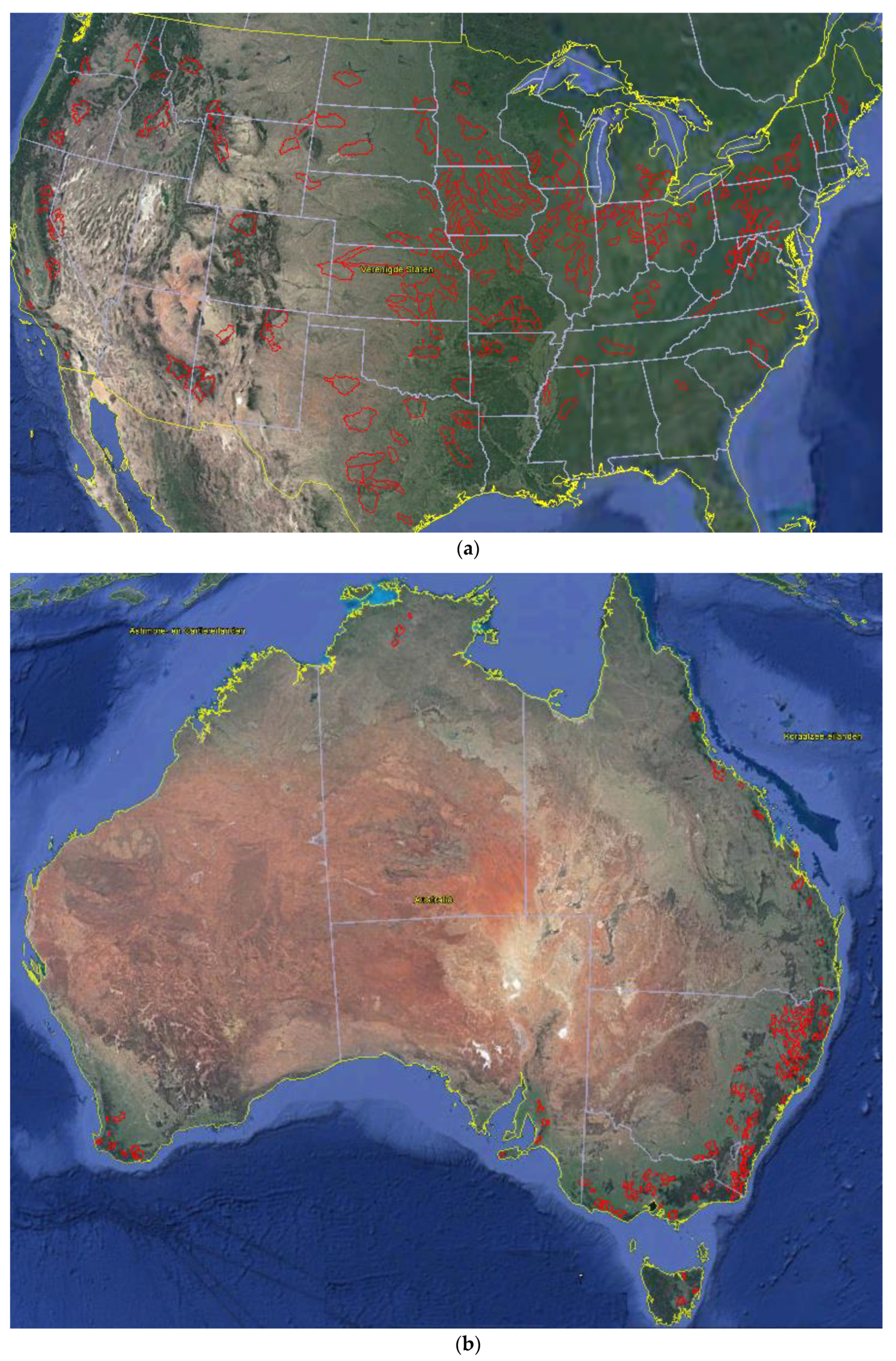
Based on these criteria, two datasets were selected: The United States (US) MOPEX dataset [20] and the Australian dataset [21]. The US dataset includes 431 catchments of which 265 are meeting the criteria. The Australian dataset includes 331 catchments of which 207 are meeting the criteria. This results in 472 catchments selected for this study and shown in Figure 1.
The catchments in the US MOPEX dataset are supposed to be unaffected by upstream regulation and have surface areas between 150 and 10,000 km2. Daily precipitation, minimum and maximum temperature, and discharge data are present in the MOPEX dataset. Missing values in the precipitation dataset were completed by MOPEX using neighbouring stations. Minimum and maximum temperature values for some time instants were switched to repair erroneous, mixed minimum and maximum values. Other catchment characteristics present in the dataset are elevations of the measuring stations, catchment boundaries, streams, soils (texture, hydraulic properties, etc.), vegetation (type, rooting depth, phenology, etc.), geology, snow cover and climatological potential evapotranspiration values. The potential evapotranspiration (PET) is determined using the Hargreaves equation [22] with the minimum and maximum temperature as input. These PET values are corrected using the monthly climatological PET values from the MOPEX dataset.
The catchments in the Australian dataset are unaffected by upstream regulation or diversion and have surface areas between 50 and 2000 km2. Gridded monthly precipitation was derived by interpolation of over 6000 daily precipitation stations in Australia. These data were converted to daily precipitation by using the daily precipitation distribution from the nearest station. The catchment average daily precipitation was estimated by averaging over the grid cells within the catchment [21]. Only monthly climatological potential evapotranspiration values for each catchment are available. However, the interannual variability of the monthly potential evapotranspiration is small, since the coefficient of variation of monthly values is smaller than 0.05 [21]. In the MOPEX dataset, only seven catchments have a coefficient of variation higher than 0.05 (maximum 0.055) and hence the interannual variability of monthly potential evapotranspiration values is similar for the Australian and US catchments. The influence of the interannual variability will be assessed by comparing the results of the attribution method for the US using temporally varying and climatological potential evapotranspiration values. Discharge data are present in the Australian dataset for at least 10 years, in line with one of the criteria in this study. Other catchment characteristics present in the dataset are catchment surface areas, catchment boundaries, and mean annual precipitation and discharge.
2.2. Attribution of Changes in Streamflow
The attribution of changes in streamflow comprises four steps. First, the trends in annual discharge series will be analysed. Second, the time series will be split into two parts for application of the attribution method. Third, the attribution method will be applied and fourth, the results will be evaluated based on the significance of the outcomes and considering different catchment characteristics.
The Mann–Kendall test [23,24] will be used for trend detection. If this test detects a trend in the annual discharge series, the attribution method can be used to determine whether this change has been caused by climate and/or land-use changes. If no trend is present, it is still possible that climate and land-use changes had (probably compensating) effects on the discharge. Sen’s slope estimator [25] will be used to determine the slope and direction of a trend.
The discharge time series is split into two parts, one at the beginning and one at the end of the measuring period representing a pre-change and post-change period, respectively. Only these two periods will be considered, independent of the total length of the time series. The length of the periods is the same for each catchment and at least five years and mostly ten years.
The attribution method of Tomer and Schilling [13] is used, which separates the effects of land use and climate change on streamflow by making use of changes in the proportion of excess water relative to changes in the proportion of excess energy on an annual scale. Excess water is calculated by subtracting the actual evapotranspiration (ET) from the precipitation (P) within a catchment. The actual evapotranspiration is determined from the difference between precipitation and discharge for a hydrological year to minimize the influence of fluctuations in water storage on the water balance. Excess water divided by the available water (P) gives the dimensionless value Pex. Excess energy is calculated by subtracting the actual evapotranspiration from the potential evapotranspiration (PET). Excess energy divided by the available energy (PET) gives the dimensionless value Eex. The values of Pex and Eex vary between 0 and 1 representing no excess water or energy in the system and maximum excess water or energy in the system, respectively.
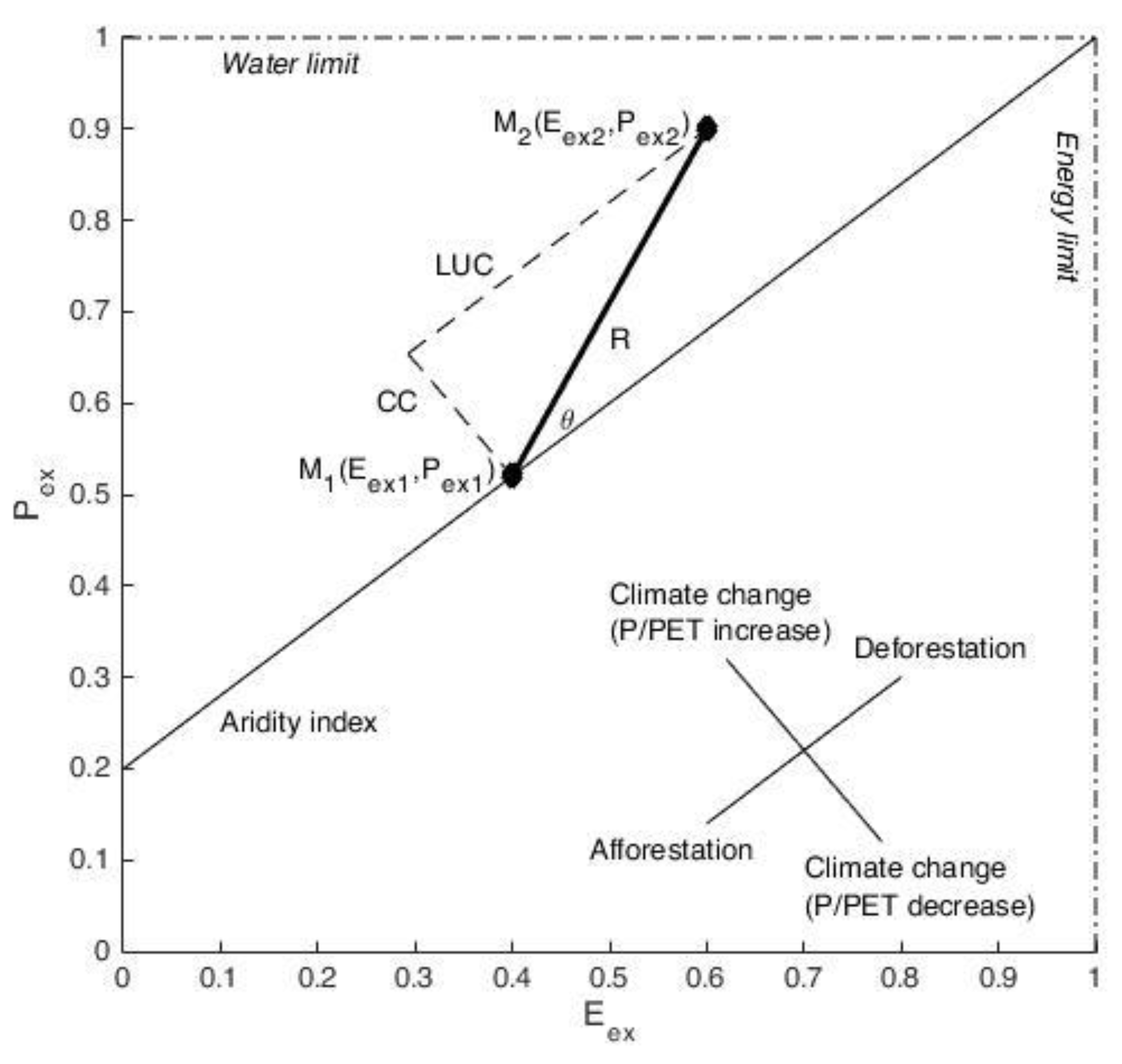
The indicators for proportions of excess water and energy are sensitive to climate change and land use change, which is an important assumption for this method. Changes in vegetation will directly affect ET, but not P and PET, which result in increasing or decreasing Pex and Eex, both in the same direction. Therefore, changes in land use, related to vegetation, will affect Pex and Eex in the same direction (increasing or decreasing). However, the influence of climate change on these parameters is different. Changes in climate are considered to affect p and PET, but not ET at a regional scale. This leads to increased Pex and decreased Eex in case of an increased P/PET ratio with time, or to decreased Pex and increased Eex in case of a decreased P/PET ratio with time. The shift in time of the parameters Pex and Eex is visualized in Figure 2. The direction of change indicates the driving force of the change in discharge. The direction of change is relative to the aridity index as Renner et al. [9] added to the attribution method of Tomer and Schilling [13] to enable the application of the method to all climatic conditions. Without this addition the method only is applicable to regions where precipitation demands equal evaporative demands. The aridity index is the ratio between the long-term average PET and P. A shift parallel to the aridity index indicates land use change as the driving force of the changing discharge, because this indicates only ET has changed. A shift perpendicular to the aridity index indicates climate change as the driving force of the changing discharge, because this means only the ratio of PET and P has changed. A shift parallel to the aridity index to higher Pex and Eex values indicates an increased ET, which is the case when an increased amount of vegetation is present. A shift to lower Pex and Eex values indicates a decreased ET, which is the case when a decreased amount of vegetation is present.
The contributions of climate change (CC) and land use change (LUC) can be determined from Figure 2 through geometric calculations [12]. The calculation of CC and LUC is slightly adapted to incorporate the direction of the shift in order to enable application to a large number of catchments. A shift in the afforestation (deforestation) direction of Figure 2 will be indicated with a negative (positive) value for the contribution of land use change. A shift in the P/PET increase (P/PET decrease) direction of Figure 2 will be indicated with a negative (positive) value for the contribution of climate change.
The results of the attribution method will be particularly interesting when there is a significant change between the pre-change period (M1 in Figure 2) and the post-change period (M2). The values of M1 and M2 are averages of 5 to 10 points (the number of years in the two considered periods) and are described by two variables (Pex, Eex). A method to test whether one group of two-dimensional observations is different from another group of two-dimensional observations is the Fasano and Franceschini test [26]. This test is an extension of the Kolmogorov–Smirnov test and is applicable to any kind of unknown distribution. The level of significance used is 95% in line with earlier statistical tests.
The catchments will be classified based on available catchment characteristics to present and evaluate the results of the attribution analysis. The first characteristic is the catchment size, since it is known that relations between land-use changes and streamflow changes are harder to find for large catchments [6]. The second characteristic is historical land use, because of its relationship with land use change. For instance, deforestation will likely not take place in desert areas. The third characteristic is the average catchment slope, since it influences the residence time of water in a catchment and hence the vulnerability of streamflow to changes in climate and land use. The fourth characteristic is the climate, which will be described by means of the updated Köppen classification [27] and the aridity index, which is also used to calculate CC and LUC.
2.3. Evaluation of Attribution Method
The attribution method will be evaluated by using observed trends in documented land-use changes and determining the influence of the length of the data series on the results.
Documented land-use changes [28,29,30,31,32,33] will be compared with results of the attribution method. This will be done for the catchments with the five highest and five lowest significant values for LUC. This procedure will also be applied for the five catchments with LUC values closest to zero, where according to the attribution method no land-use changes should have occurred.
The catchments will be classified based on the length of the data series to assess whether a longer measuring period results in larger LUC and CC values.
In addition, the influence of the interannual variability of monthly potential evapotranspiration will be assessed by comparing the results of the attribution method for the US using temporally varying and climatological potential evapotranspiration values (see Section 2.1).
3. Results
3.1. Attribution of Changes in Streamflow
The Mann–Kendall test showed for 81 American and 86 Australian catchments a significant trend in the annual discharge. Most of the discharge trends in American catchments are positive (74 out of 81), while most trends in Australian catchments are negative (85 out of 86). The presence of a trend will be used to make a distinction between catchments in subsequent analyses.
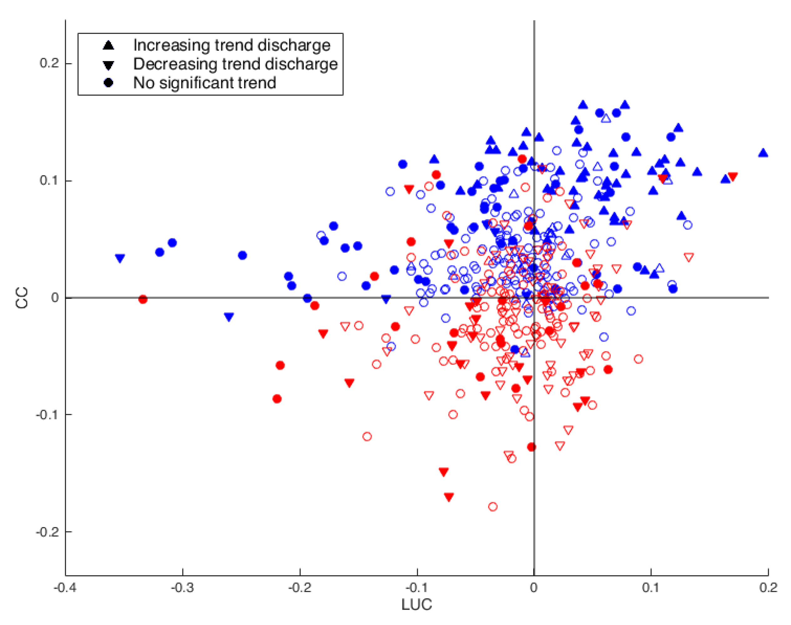
The results of the attribution method are presented in Figure 3 and Figure 4. Figure 3 shows the results for all catchments and Figure 4 shows the results classified by country, trend in discharge (positive, negative or not significant) and (non-)significance of LUC and/or CC values based on the Fasano and Franceschini test. This latter test shows that 61 out of the 81 American catchments and 21 out of the 86 Australian catchments have significant LUC and/or CC values.
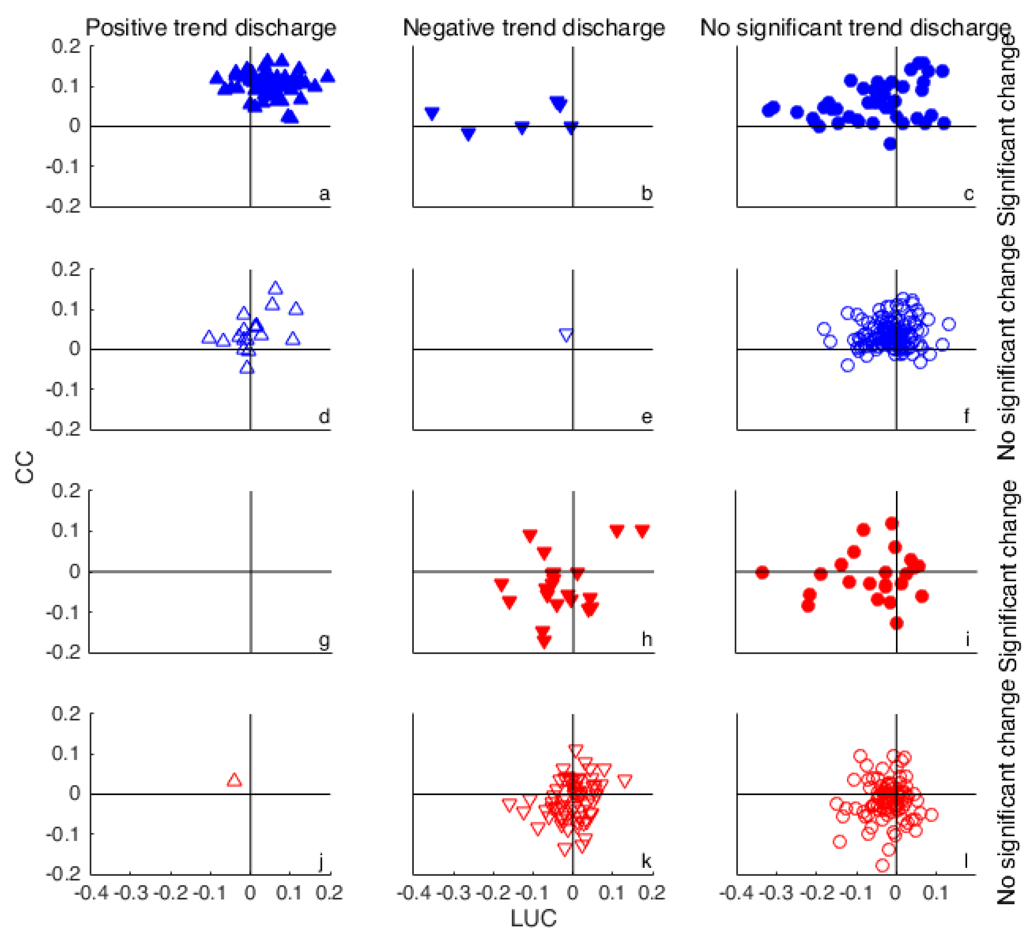
The difference between the two countries is the most obvious one. The American catchments hardly have negative values for CC, while many Australian catchments have CC values between −0.2 and 0. This indicates that the ratio P/PET for nearly all catchments in the US is increasing, while in Australia it is increasing and decreasing. The second observation is the trend in the discharge. A positive discharge trend (Figure 4a,d,g,j) is shown for catchments with higher values for CC than catchments with a negative discharge trend (Figure 4b,e,h,k). Catchments without a significant discharge trend (Figure 4c,f,i,l) have CC and LUC values in a wider range: close to the origin as well as further away and in all directions. Furthermore, catchments with significant CC and/or LUC values (Figure 4a–c,g–i) are located further from the origin than catchments without significant CC and/or LUC values (Figure 4d–f,j–l).
In Figure 4a, mostly positive LUC and CC values are present, which means a positive discharge trend is the result of deforestation (positive LUC values) and a wetter climate (positive CC values). In Figure 4b,h, mostly negative LUC and CC values are shown. This means that a negative discharge trend is the result of afforestation (negative LUC values) and a drier climate (negative CC values). For the Australian catchments the changing climate is a more important factor for the negative discharge trend than for the American catchments.
In Figure 4b,h, some catchments are located very close to origin, meaning neither CC nor LUC are influencing the streamflow while a (negative) discharge trend is present. However, Figure 5 shows that the slope of the discharge trend, estimated with Sen’s slope estimator, is smaller than 1 mm/y. The trend still is significant, because the variation is relatively small and the length relatively long. This makes it easier to detect a trend, despite its small slope. In Figure 4h also some positive values for CC and LUC are shown, which is not expected. The corresponding decreasing discharge trends also have a smaller slope than 1 mm/year.
In Figure 4c two catchments are located relatively far from the origin, while there is no significant discharge trend. This is a result of the very large variation of the annual discharge making it hard to detect a trend, although the slope is relatively large. This is also the case for the Australian catchment shown in Figure 4i, located relatively far from the origin as well. Besides the large variability in the annual discharge, the length of the measuring period of this catchment is only 11 years. This low number of points makes it even harder to detect a trend in the discharge.
Figure 5 shows the American and Australian catchments with a significant discharge trend and the corresponding magnitude of the trend. American catchments with a discharge trend larger than 3 mm y−1 or lower than −3 mm y−1 are further from the origin than catchments with a smaller discharge trend. Furthermore, negative slopes tend to have negative values for LUC meaning that afforestation played an important role in decreasing the discharge. Australian catchments with a discharge trend smaller than −2 mm y−1 are further away from the origin than catchments with a smaller discharge trend.
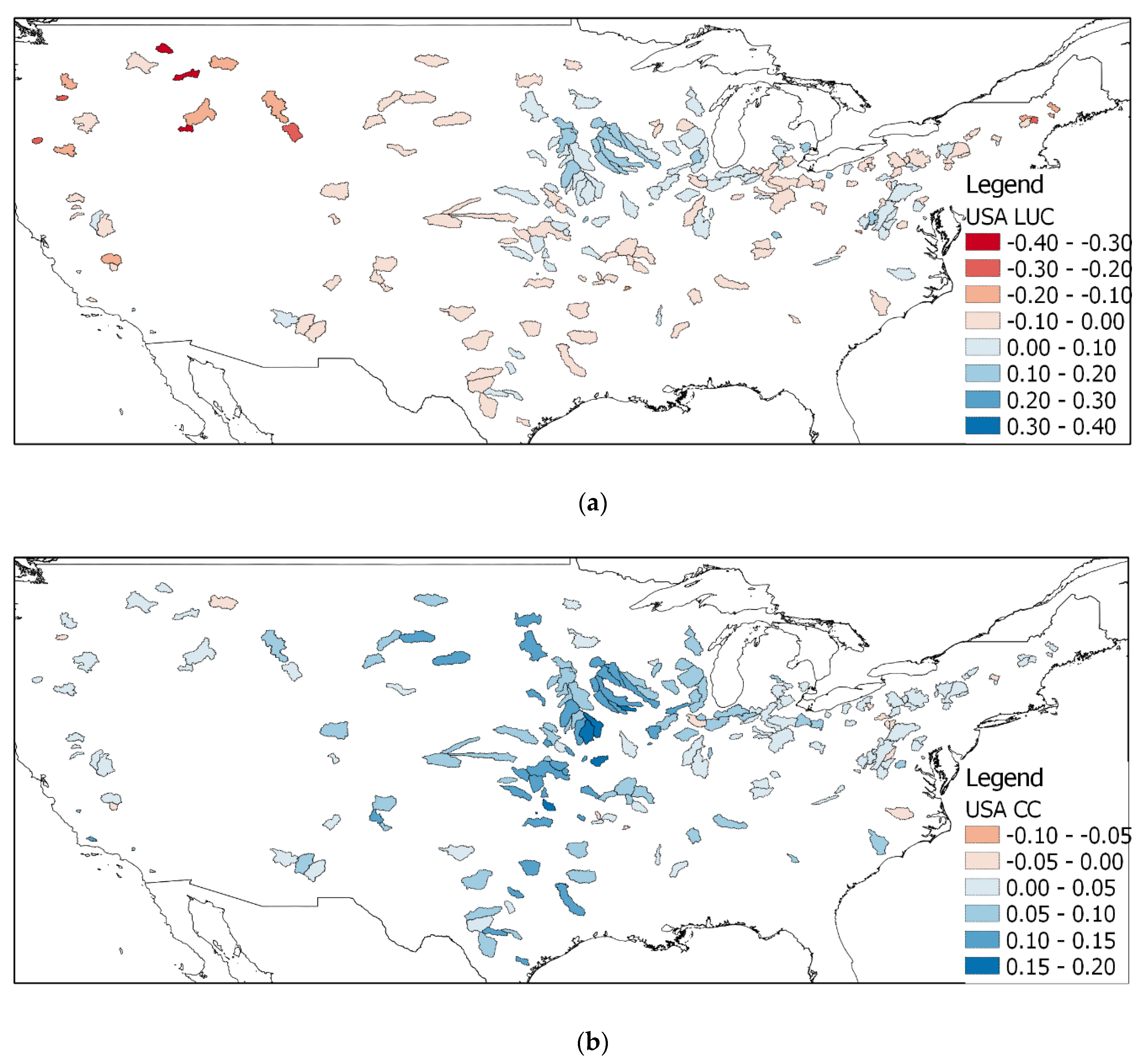
Figure 6 shows the spatial distribution of LUC and CC values of the American catchments. The catchments with the lowest LUC values are located in the northwest while the highest values particularly are located in the mid-north part of the United States. For the CC values a horizontal pattern is present. From the west to the middle the CC values increase and further to the east the values decrease again. The spatial distribution of LUC and CC values of the Australian catchments (not shown here) did not reveal any particular pattern.
3.2. Influence of Catchment Characteristics
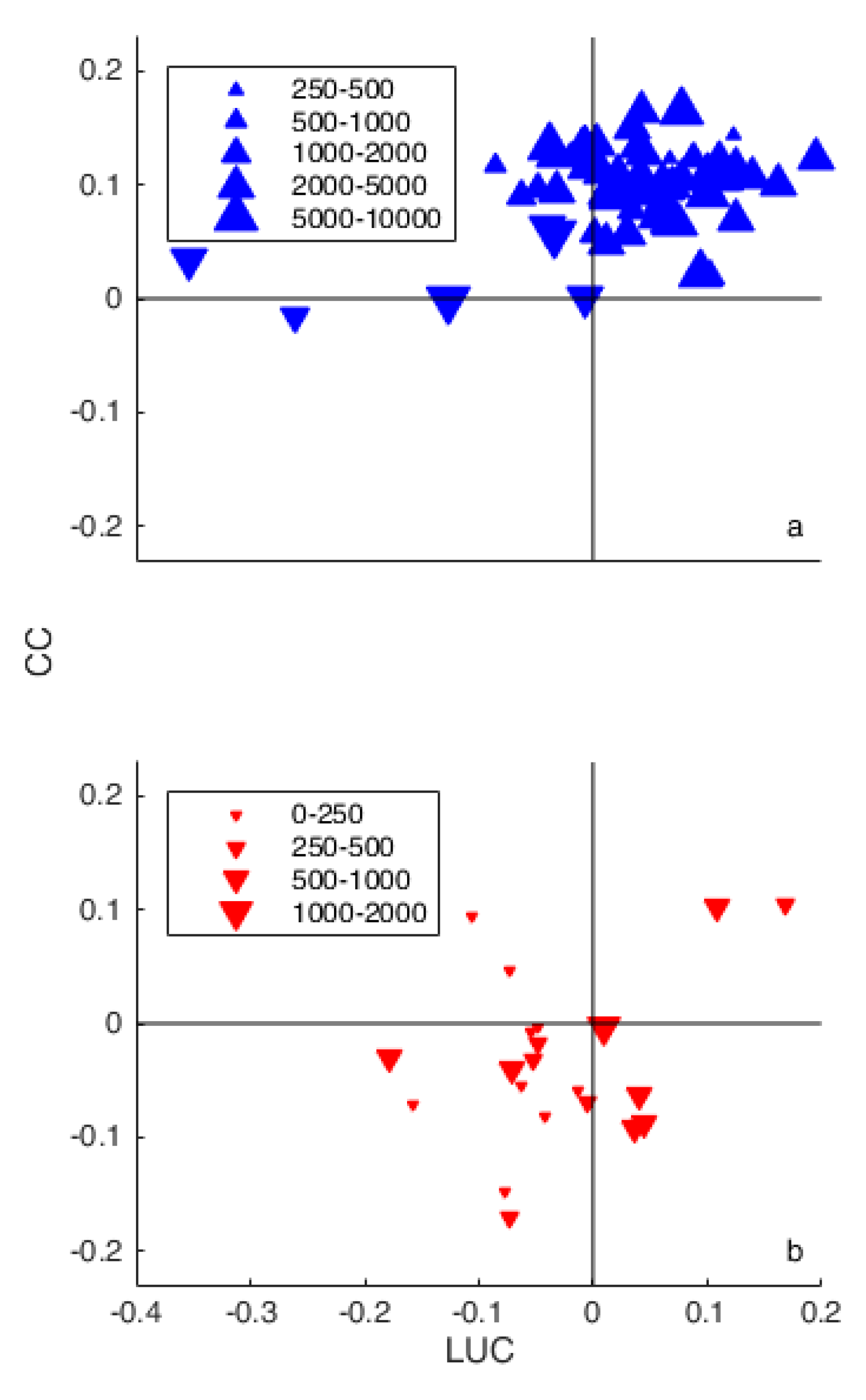
Relations between catchments characteristics and LUC and CC values are analysed to further explore and verify land-use changes, climate changes and discharge trends. Figure 7 shows the American and Australian catchments with a significant discharge trend and the corresponding surface area. Larger American catchments seem to have a relatively more significant discharge trend and significant LUC and/or CC values than smaller catchments, while this is not the case for the Australian catchments. However, a relation between the size of the catchments and the LUC and/or CC values is hard to find. An analysis of 37 nested catchments in the United States and 12 nested catchments in Australia only supported the hypothesis of increasing LUC values with decreasing catchment size for the Australian catchments. For the American catchments, this hypothesis was not supported probably due to other (local) factors.
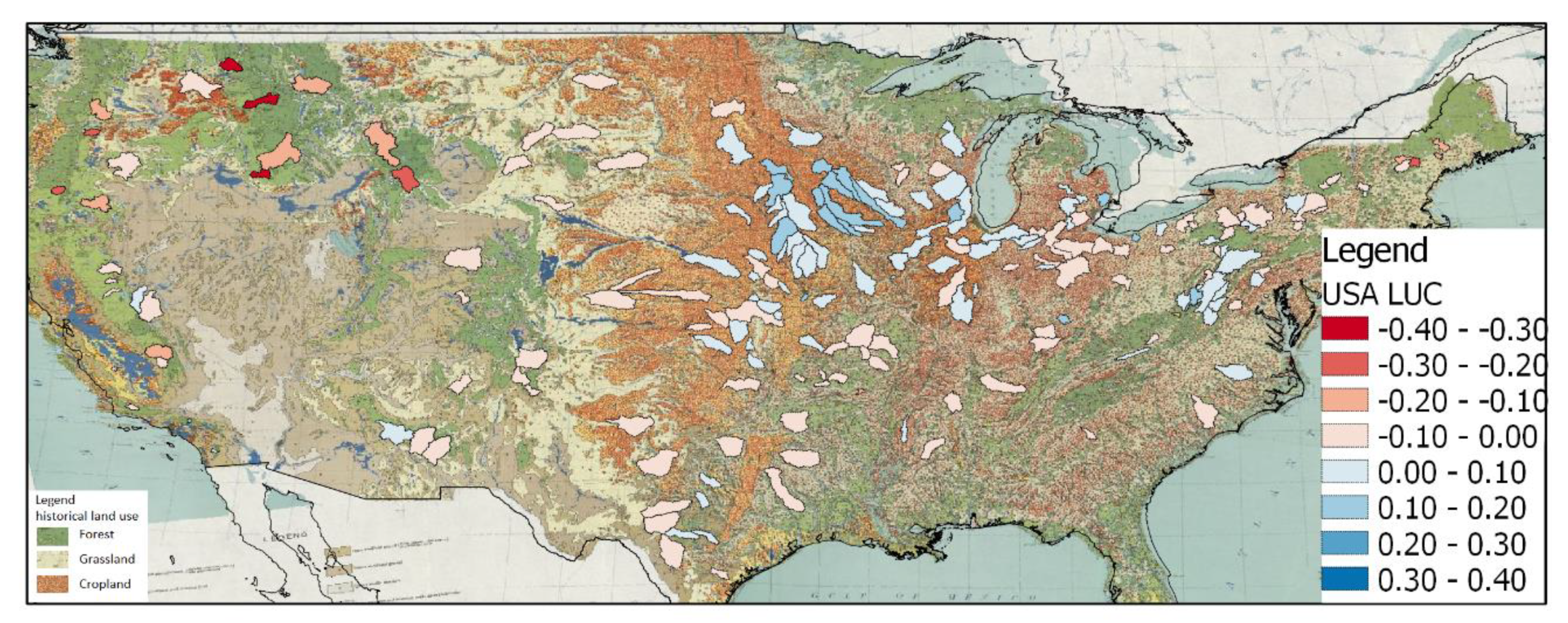
Figure 8 shows the LUC values on top of the historical land use distribution in the United States in 1950 [34]. The spatial distribution of LUC is to some extent related to the pattern as shown in the historical land use map. In the forests the LUC values are negative and in cropland the values are positive. This indicates that in the forests, afforestation has taken place, and in the croplands, deforestation. Afforestation might also include increased forages and conservation cover, and deforestation might also include conservation tillage and removal of perennials. In the middle part of the United States where grassland is present, the LUC values are close to zero, indicating that land use did not change. These observations indicate forests have become denser and cropland has become less dense. In particular the latter observation is hard to understand, because most farming activities have increased. However, this increase could have taken place in combination with deforestation although evidence is not present for this explanation. For Australia (not shown), LUC values can hardly be related to the historical land use distribution, because the LUC pattern is less clear and the resolution of the historical land use map [35] is coarse compared to the map of the United States.
It is generally believed that catchments with a relatively small water storage capacity are more sensitive to changes than catchments with a large storage capacity. The water storage capacity is related to the average catchment slope, i.e., capacities will be smaller for steeper catchments. This means that catchments with large slopes should be more sensitive to changes than catchment with small slopes [36]. Since water storage data were not available for the American and Australian catchments in this study, the slopes were used as a proxy to analyse the sensitivity of catchments to land use and climate changes in relation to the water storage capacity. The slope analysis was only done for the American catchments, because of the availability of high-resolution slope data (1 arc-second) for this part of the world from the U.S. Geological Survey [37]. For some catchments (15 out of 61) the dataset was incomplete, so the average catchment slope could not be calculated. The sensitivity of a catchment to land use and/or climate changes is quantified by the ratio of the magnitude of the discharge trends estimated by Sen’s slope estimator (S) and the LUC, CC, and resultant length (R) values. The R value represent the combined influence of land use and climate changes, see Figure 2.
Figure 9 shows the relation between the average catchment slope and the combined sensitivity (S/R). The separate sensitivities to land-use changes and climate changes are not shown, because these relations did not provide any complementary information. Figure 9 does not show a clear trend, but a weak decreasing trend might be detected rather than an expected increasing trend. This might be the result of only including relatively flat catchments (mostly slopes less than 4 degrees).
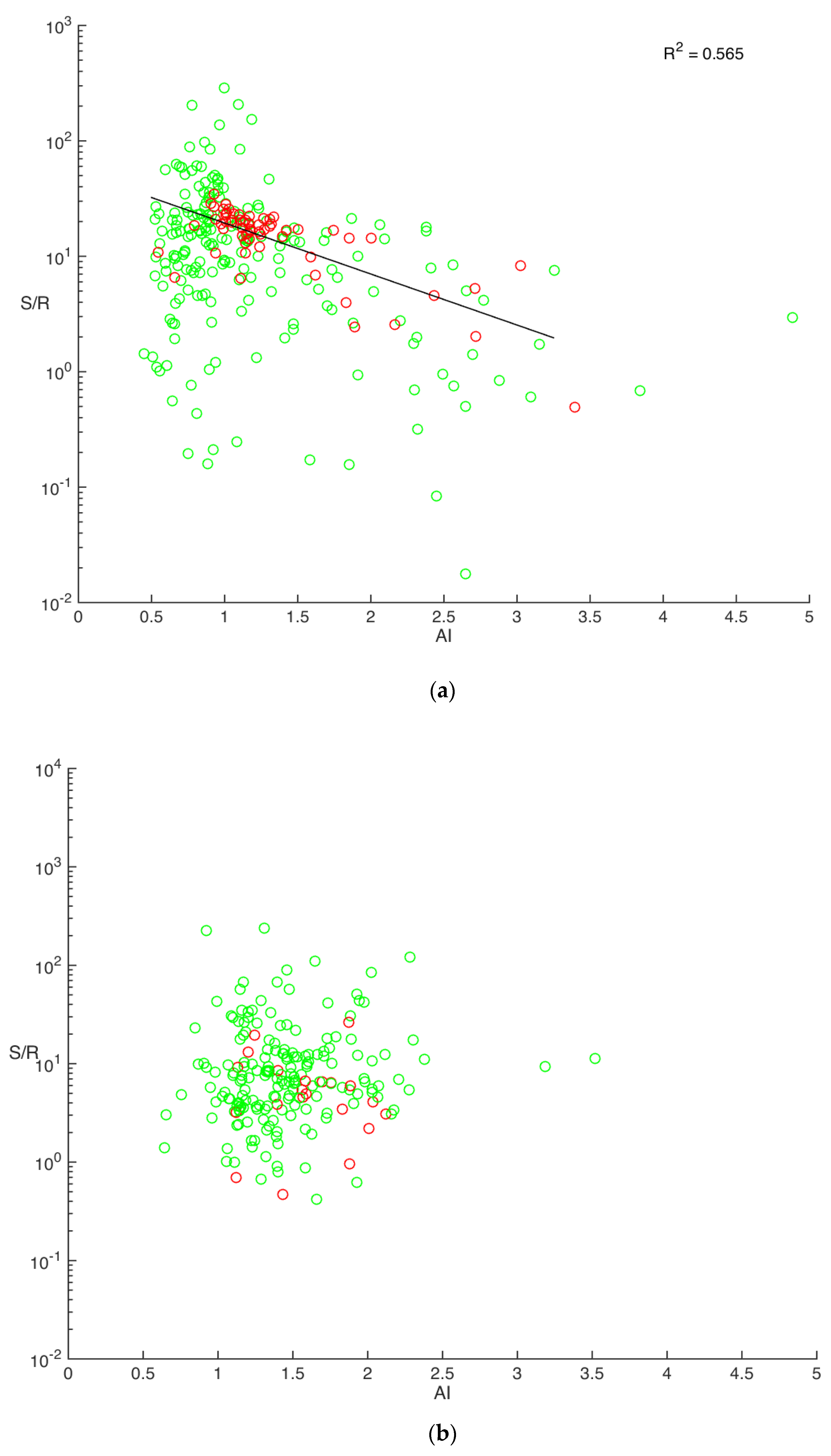
The last characteristic is the climate, which has been described by means of the updated Köppen classification and the aridity index. The CC values did not show any relation with the Köppen classification for the American and Australian catchments. The relation between the aridity index (AI) and the combined sensitivity (S/R) is shown in Figure 10. The relations for CC (and LUC) did not provide additional insight and therefore are not shown here. The relation between the aridity index and the combined sensitivity is clearer for the American catchments than the Australian catchments with a decreasing sensitivity with increasing aridity index. In wet catchments (low aridity indices) there is more room for changes, whereas in dry catchments less water is available limiting the room for possible changes.
3.3. Evaluation of Attribution Method
Evaluation of the attribution method has been carried out using documented land-use changes, analysing the influence of the measuring period on the results and determining the difference between results using climatological and variable potential evapotranspiration values.
Documented land-use changes for 15 catchments subdivided into three categories were used [28,29,30,31,32,33]. The first category includes the catchments with the lowest (negative) LUC values, which means that afforestation should have taken place. Three out of five investigated catchments show documented land-use changes, however this mostly concerns logging activities and forest fires. For two of these three catchments, regeneration of forest is reported over the measuring period. The second category includes the catchments with the highest (positive) LUC values. This means that deforestation should have taken place. Documented information is available for three out of five catchments and these sources show that in two catchments the crop production has increased during the measuring period without mentioning a possible relation with deforestation. In the third catchment logging activities took place starting in 1800, but this refers to a larger region than the single catchment. The last category includes the catchments with the lowest absolute LUC values. This means that land use change should not have taken place. Documented land-use changes do not mention anything about land-use changes for all five catchments. Although information on historic land-use changes is incomplete, it can be concluded that documented land-use changes are not always as expected given the results of the attribution method.
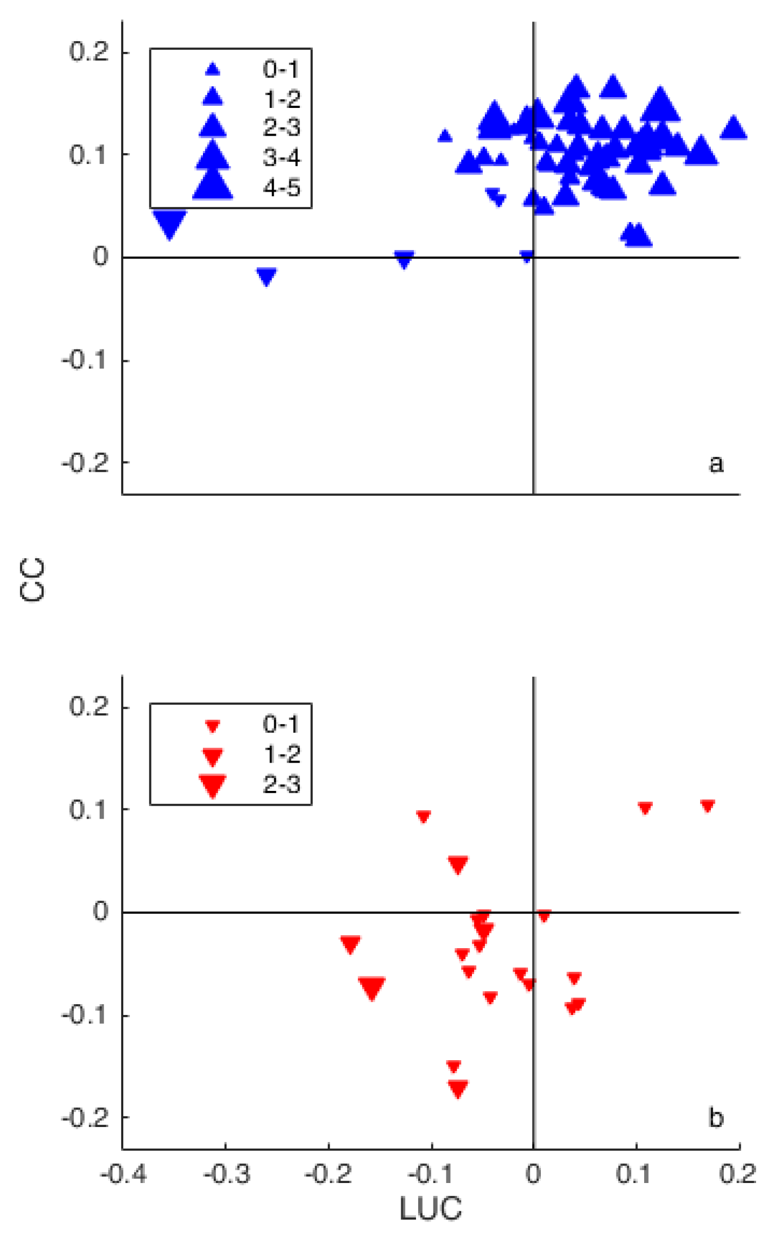
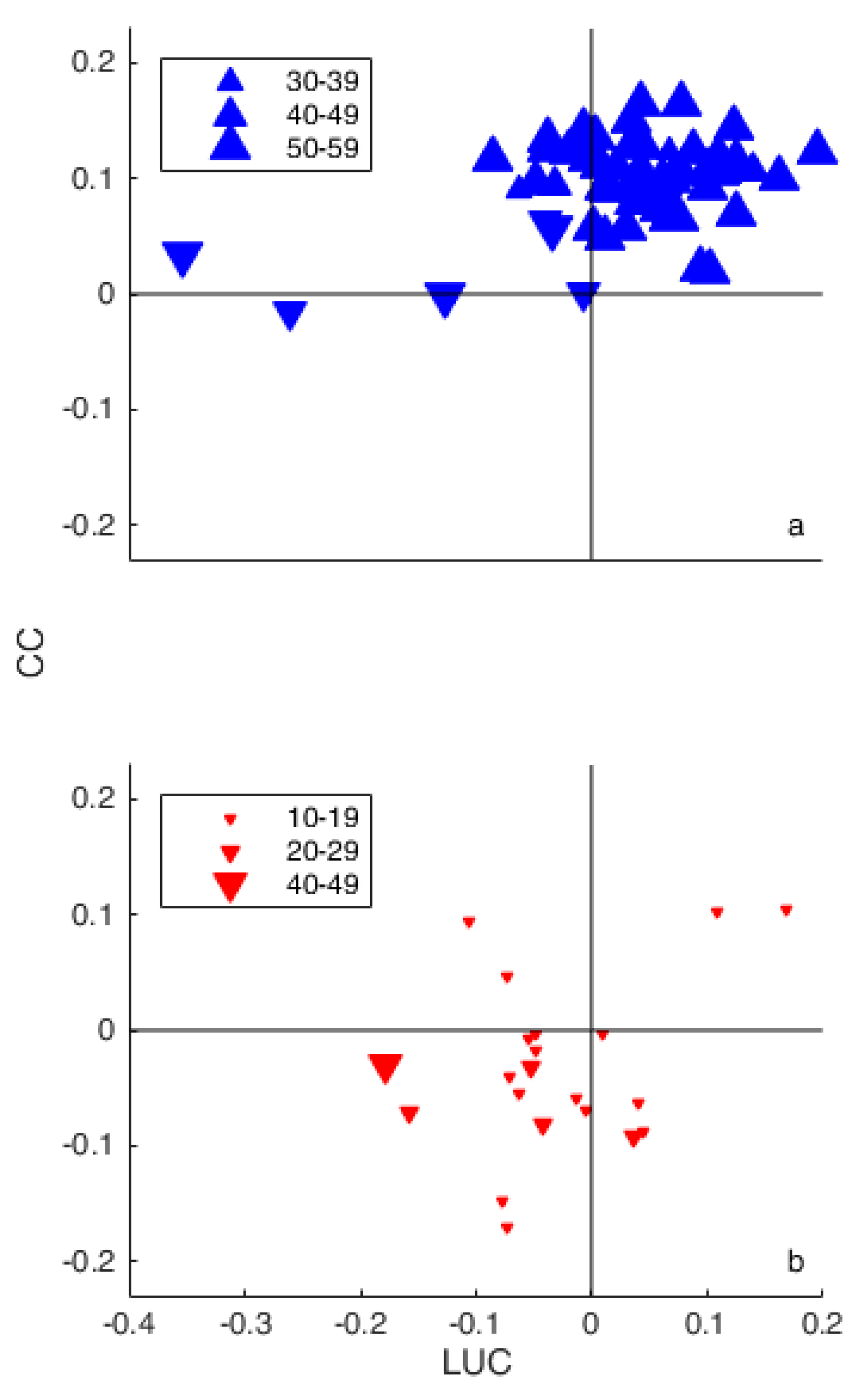
Figure 11 shows the length of the measuring periods for the American and Australian catchments with a significant discharge trend and significant LUC and/or CC values. The figures do not show a clear pattern, which is partly because nearly all catchments have measuring periods of 50 to 59 years and 10 to 19 years for the American and Australian catchments, respectively. The hypothesis is that a longer measuring period generally will result in larger changes, but this can be hardly confirmed based on the patterns in Figure 11.
Figure 12 shows the differences between the results of the attribution method using climatological and variable potential evapotranspiration (PET) values for all American catchments. The LUC and CC values calculated using variable PET are subtracted from the LUC and CC values calculated using climatological PET values. Most catchments have a negative difference for CC and a positive difference for LUC. This means that when using constant PET values lower CC values and higher LUC values are obtained, i.e., that there is less deforestation and less decrease in P/PET ratio than estimated with variable PET values. The differences are relatively small, only up to 0.04 for both LUC and CC values. The Cfa climate of the Köppen climate classification is used to compare the American catchments with the Australian ones so that the climatic conditions are more comparable, because in both countries quite a lot of catchments are present in this climate class. The differences for this climate are comparable to differences for other climates, so it seems that the climate conditions do not influence the differences between results using variable and climatological PET values. In conclusion, although there are small differences in results using variable and constant PET values, attribution results are similar and useful as long as the coefficient of variation of PET is relatively small (i.e., smaller than 0.05).
4. Discussion
4.1. Comparison with Previous Studies
The results of this study are compared with the large sample study of Wang and Hejazi [15] for the United States, since that study also used the MOPEX dataset (totally 431 catchments). The spatial patterns of the results for the United States and the influence of the aridity index on the results are compared. In addition, the results are compared with other relevant studies.
The spatial patterns are compared through the spatial distributions of the contribution of climate change (CC) and land use change (LUC). The higher (positive) values of CC are located in both studies in the middle part of the US, while negative values are particularly located in the north-western part. The highest (positive) LUC values are located in the middle north in both studies. However, the lowest (negative) values are located in the middle part of the US according to Wang and Hejazi [15] and in the north-western part according to this study. Differences may be attributed to differences in methods in both studies. First, the sample sets of catchments are different due to different selection criteria. Second, the methods of splitting the time series are different, where Wang and Hejazi [15] used a single year as change point resulting in long pre-change and post-change periods. However, the change point seems to be rather arbitrary and two long, connected periods might prevent identification of the main hydrological changes. Third, the applications of the attribution method are different. Wang and Hejazi used equations to determine the Budyko curve, where a single parameter was calibrated on the pre-change period. The method of Tomer and Schilling used in this study did not require calibration.
The influence of the aridity index on the results of both studies might further explain differences between spatial patterns. Wang and Hejazi [15] show clear relations between climate and human induced streamflow changes and the aridity index, where streamflow changes increase with an increasing aridity index. Based on these findings, they conclude that arid regions are more vulnerable for climate and land use change induced changes in streamflow than wet regions. In this study we found an opposite relation, but this can be related to the different approaches used to determine the sensitivity. Wang and Hejazi used absolute values to quantify the change in discharge and corresponding sensitivities, where we used relative values.
The main findings of this study for the United States and Australia, i.e., a positive (negative) trend in annual discharge is caused by deforestation (afforestation) and a wetter (drier) climate, are in line with results of many studies in other parts of the world. For instance, Benito et al. [38] observed increases in runoff with deforestation for small sites in Spain, Coe et al. [39] found increases in streamflow with deforestation for a large basin in East-Central Brazil and Levy et al. [40] reported an increase in dry season low flow with deforestation for 324 river basins in Brazil. For afforestation, García-Ruiz and Lana-Renault [41] found decreases in runoff for most of Europe and Keesstra [42] and Cerdà et al. [43] came to similar conclusions for catchments in Slovenia and Spain, respectively. Numerous studies have shown that a wetter (drier) climate leads to increases (decreases) in runoff, for example for west Africa [44], 24 major river basins in the world [45] and the upstream part of the Yellow River basin [14].
4.2. Potential of Attribution Method
The potential of the attribution method of Tomer and Schilling [13] clearly is its applicability to large sample sets of catchments. In addition to the adaptations by Renner et al. [9] and Marhaento et al. [12], three extensions of the method were introduced to enable large scale application. First, a distinction was made between catchments with and without a significant discharge trend using the Mann–Kendall test and the magnitude of the change in discharge was assessed using Sen’s slope estimator. Second, the actual values of LUC and CC are calculated instead of relative contributions of climate and land use change as Marhaento et al. [12] did. This avoids the loss of information on the direction of change and enable a better comparison between catchments. Third, a distinction was made between catchments with and without a significant difference in excess water and energy between the pre-change and post-change period using the Fasano and Franceschini test. This revealed significant contributions of land use and/or climate change to changes in discharge.
The attribution method has been applied to American catchments using time-varying potential evapotranspiration (PET) values and to Australian catchments using climatological values. In order to assess the effect of using climatological vs. time-varying PET values, we compared the results of the attribution method for American catchments using both types of PET values. Results were similar and useful as long as the coefficient of variation of PET is smaller than 0.05. This means that the attribution method could also be used in other regions where time-varying PET data are scarce and the interannual variability of PET is low.
4.3. Limitations of Attribution Method
Two basic assumptions of the attribution method can influence the results. First, it is assumed that land-use changes will affect the actual evaporation and climate change will affect precipitation and/or potential evapotranspiration. This might not always be correct, since climate change might affect actual evapotranspiration to some extent as well, in particular for larger catchments. Renner et al. [12] applied the attribution method in Germany and found some land use related hydrological changes in sub-catchments where no deforestation or other land-use changes were detected. Hence, this assumption might lead to an overestimation of the contribution of land use change and an underestimation of the contribution of climate change. Second, it is assumed that changes in water storage can be neglected in the calculation of the annual water balance. Although the water balance is determined for hydrological years, there might be catchments where these changes are relatively large, in particular small catchments with relatively large groundwater systems and contributions from groundwater.
4.4. Generalisation
The attribution method is applicable to each catchment as long as time series of precipitation, potential evapotranspiration and discharge are available for a period of at least 10 years. Furthermore, a change point or trend in the time series of the annual discharge is needed to attribute changes in land use and/or climate to changes in streamflow. It is recommended to check whether changes in water storage over the years are relevant in a catchment by using for instance remote sensing products such GRACE data [46]. This might lead to more accurate actual evapotranspiration values and an increased reliability of the results.
It is expected that similar catchments will provide similar results. The similarity of catchments depends on the location, the aridity and the historical land use, but also on the water storage capacity of the catchment. It is expected that the higher the water storage capacity the less sensitive the catchment is to changes, however this statement should be validated with more in-depth studies for a small number of catchments.
5. Conclusions
The objective of this study was to apply a coupled water–energy budget approach, to attribute changes in streamflow to climate change and land use change, to a large sample set of catchments in Australia and the United States and to evaluate the used method based on catchment characteristics and using historical land use. It can be concluded that if a positive (negative) significant trend in annual discharge is present and the contribution of land use change and/or climate change is significant, this is caused by deforestation (afforestation) and a wetter (drier) climate in most cases. These results are as expected and partly confirm the applicability of the attribution method to a large sample set of catchments. When no significant trend in annual discharge is present, the results are spread over a wider range. Catchments without a significant contribution of land use change and/or climate change have smaller values for both LUC and CC.
Drier catchments are less sensitive to changes in streamflow due to climate and land-use changes than wetter catchments. Historical land use is an important indicator for the contribution of land use change. Deforestation is the main driver for changes in streamflow when agricultural activities took place during the starting period of the measurements. Afforestation is the main driver when forest was the main land use in the past in the United States.
The attribution method was evaluated based on documented land-use changes, which are in particular found for catchments of which the LUC values are high or low. For catchments with LUC values close to zero no documented land-use changes were present.
Author Contributions
M.J.B., T.C.S. and H.M. designed the research; T.C.S. performed the research; M.J.B., T.C.S. and H.M. analysed the results; and M.J.B., T.C.S. and H.M. wrote the paper.
Funding
H.M. was supported by the Directorate General of Higher Education, Ministry of Research, Technology and Higher Education of the Republic of Indonesia, grant number BPPLN DIKTI 2013.
Acknowledgments
The authors acknowledge Murray Peel from the University of Melbourne for assisting with the data for the Australian catchments. The comments of two anonymous reviewers and the editor are gratefully acknowledged and helped to improve the manuscript.
Conflicts of Interest
The authors declare no conflict of interest.
References
- Mason, S.J.; Waylen, P.R.; Mimmack, G.M.; Rajaratnam, B.; Harrison, J.M. Changes in extreme rainfall events in South Africa. Clim. Chang. 1999, 41, 249–257. [Google Scholar] [CrossRef]
- Plummer, N.; Salinger, M.J.; Nicholls, M.J.; Suppiah, R.; Hennessy, K.J.; Leighton, R.M.; Trewin, B.; Page, C.M.; Lough, J.M. Changes in climate extremes over the Australian region and New Zealand during the twentieth century. Clim. Chang. 1999, 42, 183–202. [Google Scholar] [CrossRef]
- Alpert, P.; Ben-Gai, T.; Baharad, A.; Benjamini, Y.; Yekutieli, D.; Colacino, M.; Diodato, L.; Ramis, C.; Homar, V.; Romero, R.; et al. The paradoxical increase of Mediterranean extreme daily rainfall in spite of decrease in total values. Geophys. Res. Lett. 2002, 29, 1–31. [Google Scholar] [CrossRef]
- Villarini, G.; Smith, J.A.; Baeck, M.L.; Vitolo, R.; Stephenson, D.B.; Krajewski, W.F. On the frequency of heavy rainfall for the Midwest of the United States. J. Hydrol. 2011, 400, 103–120. [Google Scholar] [CrossRef]
- Tian, Y.; Xu, Y.-P.; Booij, M.J.; Lin, S.; Zhang, Q.; Lou, Z. Detection of trends in precipitation extremes in Zhejiang, east China. Theor. Appl. Climatol. 2012, 107, 201–210. [Google Scholar] [CrossRef]
- Blöschl, G.; Ardoin-Bardin, S.; Bonell, M.; Dorninger, M.; Goodrich, D.; Gutknecht, D.; Matamoros, D.; Merz, B.; Shand, P.; Szolgay, J. At what scales do climate variability and land cover change impact on flooding and low flows? Hydrol. Process 2007, 21, 1241–1247. [Google Scholar] [CrossRef]
- Romanowicz, R.J.; Booij, M.J. Impact of land use and water management on hydrological processes under varying climatic conditions. Phys. Chem. Earth 2011, 36, 613–614. [Google Scholar] [CrossRef]
- Marhaento, H.; Booij, M.J.; Hoekstra, A.Y. Hydrological response to future land-use change and climate change in a tropical catchment. Hydrol. Sci. J. 2018, 63, 1368–1385. [Google Scholar] [CrossRef] [Green Version]
- Renner, M.; Brust, K.; Schwärzel, K.; Volk, M.; Bernhofer, C. Separating the effects of changes in land cover and climate: A hydro-meteorological analysis of the past 60 yr in Saxony, Germany. Hydrol. Earth Syst. Sci. 2014, 18, 389–405. [Google Scholar] [CrossRef]
- Zhang, M.; Wei, X.; Sun, P.; Liu, S. The effect of forest harvesting and climatic variability on runoff in a large watershed: The case study in the Upper Minjing River of Yangtze River basin. J. Hydrol. 2012, 464–465, 1–11. [Google Scholar] [CrossRef]
- Wang, X. Advances in separating effects of climate variability and human activity on stream discharge: An overview. Adv. Water Resour. 2014, 71, 209–218. [Google Scholar] [CrossRef]
- Marhaento, H.; Booij, M.J.; Hoekstra, A.Y. Attribution of changes in stream flow to land use change and climate change in a mesoscale tropical catchment in Java, Indonesia. Hydrol. Res. 2017, 48, 1143–1155. [Google Scholar] [CrossRef]
- Tomer, M.D.; Schilling, K.E. A simple approach to distinguish land-use and climate-change effects on watershed hydrology. J. Hydrol. 2009, 376, 24–33. [Google Scholar] [CrossRef]
- Zheng, H.; Zhang, L.; Zhu, R.; Liu, C.; Sato, Y.; Fukushima, Y. Responses of streamflow to climate and land surface change in the headwaters of the Yellow River Basin. Water Resour. Res. 2009, 45, W00A19. [Google Scholar] [CrossRef]
- Wang, D.; Hejazi, M. Quantifying the relative contribution of the climate and direct human impacts on mean annual streamflow in the contiguous United States. Water Resour. Res. 2011, 47, W00J12. [Google Scholar] [CrossRef]
- Wei, X.; Zhang, M. Quantifying streamflow change caused by forest disturbance at a large spatial scale: A single watershed study. Water Resour. Res. 2010, 46, W12525. [Google Scholar] [CrossRef]
- Rientjes, T.H.M.; Haile, A.T.; Kebede, E.; Mannaerts, C.M.M.; Habib, E.; Steenhuis, T.S. Changes in land cover, rainfall and stream flow in Upper Gilgel Abbay catchment, Blue Nile basin–Ethiopia. Hydrol. Earth Syst. Sci. 2011, 15, 1979–1989. [Google Scholar] [CrossRef]
- Zhang, X.; Zhang, L.; Zhao, J.; Rustomji, P.; Hairsine, P. Responses of streamflow to changes in climate and land use/cover in the Loess Plateau, China. Water Resour. Res. 2008, 45, W00A07. [Google Scholar] [CrossRef]
- Zhang, Y.; Guan, D.; Jin, C.; Wang, A.; Wu, J.; Yuan, F. Impacts of climate change and land use change on runoff of forest catchment in northeast China. Hydrol. Process 2014, 28, 186–196. [Google Scholar] [CrossRef]
- Schaake, J.; Cong, S.; Duan, Q. Large sample basin experiments for hydrological model parameterization: Results of the model parameter experiment—MOPEX. IAHS Publ. 2006, 307, 9–28. [Google Scholar]
- Peel, M.C.; Chiew, F.H.S.; Western, A.W.; McMahon, T.A. Extension of Unimpaired Monthly Streamflow Data and Regionalisation of Parameter Values to Estimate Streamflow in Ungauged Catchments; National Land and Water Resources Audit Theme 1-Water Availability; Centre for Environmental Applied Hydrology The University of Melbourne: Melbourne, Australia, 2000. [Google Scholar]
- Hargreaves, G.H.; Samani, Z.A. Reference crop evapotranspiration from temperature. Appl. Eng. Agric. 1985, 1, 96–99. [Google Scholar] [CrossRef]
- Mann, H.B. Non-parametric tests against trend. Econometrica 1945, 13, 163–171. [Google Scholar] [CrossRef]
- Kendall, M.G. Rank Correlation Methods, 4th ed.; Charles Griffin: London, UK, 1975. [Google Scholar]
- Sen, P.K. Estimates of the regression coefficient based on Kendall’s tau. J. Am. Stat. Assoc. 1968, 63, 1379–1389. [Google Scholar] [CrossRef]
- Fasano, G.; Franceschini, A. A multidimensional version of the Kolmogorov-Smirnov test. Mon. Not. R. Astron. Soc. 1987, 225, 155–170. [Google Scholar] [CrossRef]
- Peel, M.C.; Finlayson, B.L.; McMahon, T.A. Updated world map of Köppen-Geiger climate classification. Hydrol. Earth Syst. Sci. 2007, 11, 1633–1644. [Google Scholar] [CrossRef]
- Boettcher, J. Le Sueur River—Watershed Conditions and Restoration and Protection Strategies; WRAPS Report; Pollution Control Agency: Brainerd, MN, USA, 2015. [Google Scholar]
- Bugosh, N. Lochsa River Subbasin Assessment; Lewiston Regional Office, Division of Environmental Quality: Lewiston, ID, USA, 1999.
- Lamson, K.; Clark, J.S. White River Watershed Assessment; Wasco County Soil and Water Conservation District: Dalles, OR, USA, 2004. [Google Scholar]
- Rogers, K.; Woodroffe, C.D. Working with Mangrove and Saltmarsh for Sustainable Outcomes; University of Wollongong and GeoQuest Research Centre: Wollongong, Australia, 2015. [Google Scholar]
- Rothrock, G. Watershed Overview and History North Fork Coeur d’Alene River Subbasin; Idaho Department of Environmental Quality: Boise, ID, USA, 2007.
- Simpson, N.T.; Piece, C.L.; Roe, K.L.; Weber, M.J. Boone River Watershed Stream Fish and Habitat Monitoring; Iowa State University and USGS: Ames, IA, USA, 2016.
- Marschner, F.J. Major Land Uses in the United States; U.S. Agricultural Research Service, Department of Agriculture: Washington, DC, USA, 1950.
- Australia and New Zealand Land Use, Agriculture and Minerals 1962 Map. Available online: https://www.antiquemapsandprints.com (accessed on 22 February 2019).
- Bruijnzeel, L.A. Hydrological functions of tropical forests: Not seeing the soil for trees? Agric. Ecosyst. Environ. 2004, 104, 185–228. [Google Scholar] [CrossRef]
- USGS. Available online: https://www.usgs.gov/ (accessed on 22 February 2019).
- Benito, E.; Santiago, J.; de Blas, E.; Varela, M. Deforestation of water-repellent soils in Galicia (NW Spain): Effects on surface runoff and erosion under simulated rainfall. Earth Surf. Process Landf. 2003, 28, 145–155. [Google Scholar] [CrossRef]
- Coe, M.T.; Latrubesse, E.M.; Ferreira, M.E.; Amsler, M.L. The effects of deforestation and climate variability on the streamflow of the Araguaia River, Brazil. Biogeochemistry 2011, 105, 119. [Google Scholar] [CrossRef]
- Levy, M.C.; Lopes, A.V.; Cohn, A.; Larsen, L.G.; Thompson, S.E. Land use change increases streamflow across the arc of deforestation in Brazil. Geophys. Res. Lett. 2018, 45, 3520–3530. [Google Scholar] [CrossRef]
- García-Ruiz, J.M.; Lana-Renault, N. Hydrological and erosive consequences of farmland abandonment in Europe, with special reference to the Mediterranean region—A review. Agric. Ecosyst. Environ. 2011, 140, 317–338. [Google Scholar] [CrossRef]
- Keesstra, S.D. Impact of natural reforestation on floodplain sedimentation in the Dragonja basin, SW Slovenia. Earth Surf. Process Landf. 2007, 32, 49–65. [Google Scholar] [CrossRef]
- Cerdà, A.; Rodrigo-Comino, J.; Novara, A.; Brevik, E.C.; Vaezi, A.R.; Pulido, M.; Giménez-Morera, A.; Keesstra, S.D. Long-term impact of rainfed agricultural land abandonment on soil erosion in the Western Mediterranean basin. Prog. Phys. Geogr. Earth Environ. 2018, 42, 202–219. [Google Scholar] [CrossRef]
- Roudier, P.; Ducharne, A.; Feyen, L. Climate change impacts on runoff in West Africa: A review. Hydrol. Earth Syst. Sci. 2014, 18, 2789–2801. [Google Scholar] [CrossRef]
- Nohara, D.; Kitoh, A.; Hosaka, M.; Oki, T. Impact of climate change on river discharge projected by multimodel ensemble. J. Hydrometeorol. 2006, 7, 1076–1089. [Google Scholar] [CrossRef]
- Tapley, B.; Bettadpur, S.; Watkins, M.; Reigber, C. The gravity recovery and climate experiment: Mission overview and early results. Geophys. Res. Lett. 2004, 31, 1–4. [Google Scholar] [CrossRef]
Figure 1.
Maps of (a) the United States and (b) Australia with catchments included in this study, partly based on information from [20,21].

Figure 2.
Adapted Tomer and Schilling [13] framework illustrating how the fractions of excess water and excess energy respond to climate and land-use changes. The points M1 and M2 are the fractions of excess water and energy of the pre-change period (Pex1, Eex1) and the post-change period (Pex, Eex2), respectively. The resultant length (R) is the magnitude of the combined influence of land use and climate changes.

Figure 3.
Contribution of land use change (x-axis) and climate change (y-axis) for the American (blue) and Australian (red) catchments. Filled symbols indicate a significant value of (LUC) and/or climate change (CC) and open symbols indicate a non-significant value.
Figure 3.
Contribution of land use change (x-axis) and climate change (y-axis) for the American (blue) and Australian (red) catchments. Filled symbols indicate a significant value of (LUC) and/or climate change (CC) and open symbols indicate a non-significant value.

Figure 4.
Contribution of land use change (x-axis) and climate change (y-axis) for the American (blue) and Australian (red) catchments. The first and third (second and fourth) rows include catchments with (without) significant LUC and/or CC values.
Figure 4.
Contribution of land use change (x-axis) and climate change (y-axis) for the American (blue) and Australian (red) catchments. The first and third (second and fourth) rows include catchments with (without) significant LUC and/or CC values.

Figure 5.
Contribution of land use change (x-axis) and climate change (y-axis) for (a) the American and (b) Australian catchments with a significant trend in discharge and significant LUC and/or CC values. The magnitude of the discharge trend (estimated with Sen’s slope estimator) is shown in mm y−1.

Figure 6.
Spatial distribution of LUC (a) and CC (b) values of the American catchments.

Figure 7.
Contribution of land use change (x-axis) and climate change (y-axis) for (a) the American and (b) Australian catchments with a significant trend in discharge and significant LUC and/or CC values. The surface area of the catchments is indicated by the symbol sizes and shown in km2.
Figure 7.
Contribution of land use change (x-axis) and climate change (y-axis) for (a) the American and (b) Australian catchments with a significant trend in discharge and significant LUC and/or CC values. The surface area of the catchments is indicated by the symbol sizes and shown in km2.

Figure 8.
Spatial distribution of LUC values of the American catchments on top of the historical land use distribution of 1950.
Figure 8.
Spatial distribution of LUC values of the American catchments on top of the historical land use distribution of 1950.

Figure 9.
Ratio of Sen’s slope estimator (S) and the resultant length (R) in mm yr−1 as a function of average catchment slope in degrees for the American catchments with a significant trend in discharge and significant LUC and/or CC values.
Figure 9.
Ratio of Sen’s slope estimator (S) and the resultant length (R) in mm yr−1 as a function of average catchment slope in degrees for the American catchments with a significant trend in discharge and significant LUC and/or CC values.

Figure 10.
Ratio of Sen’s slope estimator (S) and the resultant length (R) in mm yr−1 as a function of the aridity index (AI) for (a) American catchments and (b) Australian catchments. Red points indicate catchments with a significant trend in discharge and significant LUC and/or CC values and green points are the other catchments. The black trend line for the American catchments is based on the red points and the corresponding coefficient of determination (R2) is shown.

Figure 11.
Contribution of land use change (x-axis) and climate change (y-axis) for (a) the American and (b) Australian catchments with a significant trend in discharge and significant LUC and/or CC values. The length of the total measuring period is indicated by the symbol sizes and shown in years.

Figure 12.
Differences in contribution of land use change (x-axis) and climate change (y-axis) between calculating with variable and constant potential evapotranspiration values for all American catchments. Green crosses indicate a Cfa climate and blue crosses indicate other climates.
Figure 12.
Differences in contribution of land use change (x-axis) and climate change (y-axis) between calculating with variable and constant potential evapotranspiration values for all American catchments. Green crosses indicate a Cfa climate and blue crosses indicate other climates.

© 2019 by the authors. Licensee MDPI, Basel, Switzerland. This article is an open access article distributed under the terms and conditions of the Creative Commons Attribution (CC BY) license (http://creativecommons.org/licenses/by/4.0/).
Share and Cite
MDPI and ACS Style
Booij, M.J.; Schipper, T.C.; Marhaento, H. Attributing Changes in Streamflow to Land Use and Climate Change for 472 Catchments in Australia and the United States. Water 2019, 11, 1059. https://doi.org/10.3390/w11051059
AMA Style
Booij MJ, Schipper TC, Marhaento H. Attributing Changes in Streamflow to Land Use and Climate Change for 472 Catchments in Australia and the United States. Water. 2019; 11(5):1059. https://doi.org/10.3390/w11051059
Chicago/Turabian StyleBooij, Martijn J., Theo C. Schipper, and Hero Marhaento. 2019. "Attributing Changes in Streamflow to Land Use and Climate Change for 472 Catchments in Australia and the United States" Water 11, no. 5: 1059. https://doi.org/10.3390/w11051059
Note that from the first issue of 2016, this journal uses article numbers instead of page numbers. See further details here.