Exploration of the Snow Ablation Process in the Semiarid Region in China by Combining Site-Based Measurements and the Utah Energy Balance Model—A Case Study of the Manas River Basin

Abstract

Understanding the snow accumulation and melting process is of great significance for the assessment and regulation of water resources and the prevention of meltwater flooding, especially for the semiarid region in the Manas River Basin. However, the lack of long snow measurement time series in this semiarid region prevents a full understanding of the detailed local-scale snow ablation process. Additionally, the modeling of snow accumulation and melting is challenging due to parameter uncertainty. In this study, the snow ablation process in the Manas River Basin was quantitatively explored with long time-series of 3-h measurements of snow depth, snow density and snow water equivalent (SWE) at the Wulanwusu (WLWS), Hanqiazi (HQZ), and Baiyanggou (BYG) sites. This study explored the ability of the Utah energy balance (UEB) snow accumulation and melt model to simulate SWE, energy flux and water loss in the study area. Furthermore, the uncertainty in the ground surface aerodynamic roughness index z_os in the UEB model was also analyzed. The results showed that: (1) noticeable variations in snow depth, SWE and snow density occurred on seasonal and interannual time scales, and variations in melting time and melting ratios occurred on short time scales; (2) a rapid decrease in snow depth did not influence the variations in SWE, and snow melting occurred during all time periods, even winter, which is a typical characteristic of snow accumulation in arid environments; (3) the UEB model accurately simulated the snow ablation processes, including SWE, snow surface temperature, and energy flux, at WLWS, HQZ, and BYG sites; (4) the lowest contribution of net radiation to melting occurred in the piedmont clinoplain, followed by the mountain desert grassland belt and mountain forest belt, whereas the contributions of net turbulence exhibited the opposite pattern; (5) the optimal z_os in the UEB model was experimentally determined to be 0.01 m, and the UEB model-simulated SWE based on this value was the most consistent with the measured SWE; and (6) the results may provide theoretical and data foundations for research on the snow accumulation process at the watershed scale.

1. Introduction

The Tianshan Mountains are a large, high-elevation mountain range stretching across the central part of Xinjiang, China, and these mountains represent the main area of runoff formation in Xinjiang. This mountain range has complex natural geographic, hydrologic, and climatic characteristics. The winter is cold and long, and snow cover is abundant. Rapid warming in the spring leads to rapid melting of the snow cover in low- and intermediate-elevation areas and the piedmont plain, which can cause snowmelt floods and disrupt or damage traffic, animal husbandry, agricultural facilities, and people’s lives and properties [1,2]. The Manas River originates from the middle part of the northern slope of the Tianshan Mountain in Xinjiang, and snowmelt contributes significantly to spring and summer runoff in the river [3]. In recent decades, the Manas county region and surrounding areas, located in the lower Manas River, have experienced serious spring snowmelt flood disasters [4,5]. Therefore, understanding the pattern of snow accumulation and melting is of great significance to the evaluation and regulation of water resources in this region and the prevention and control of meltwater floods. Currently, research on snow in the Tianshan area has primarily focused on basin-scale remote sensing of the snow cover area [6,7,8,9], application and assessment of expanded products [10], improvement of the inversion method, simulation of the runoff sequence [11], application of the snowmelt runoff model (SRM) [4], and modification of the SRM parameters [12,13]. Although these investigations have improved the acquisition of basin-scale snow cover area and depth data, quantitative descriptions of the basin- or local-scale snow accumulation and ablation processes are lacking and are hampered by the performance of hydrological models due to the scarcity of meteorological observation stations in the region and the difficulty of accessing this region. Therefore, observation experiments and model simulations are two important means to study the pattern of snow ablation in areas with limited access and communications infrastructure.

Generally, snowmelt models can be divided into degree-day models and energy balance models. Degree-day models serve as typical statistical models and have been extensively applied in research on ice and snow melting [14]. Typical degree-day models include the Hydrologiska Fyrans Vattenbalans (HBV) model [15] and the SRM [16,17,18]. However, degree-day models have some limitations. When these models are used for different basins, the model parameters must be calibrated to the specific basin. However, the development, formation, and melting statuses of glaciers and snow differ on mountains and plains, and ground observations are difficult to collect in high and cold mountain areas. Therefore, the empirical and semiempirical parameters of the degree-day factors in the models are difficult to obtain, which leads to uncertain outcomes. Even when empirical numerical simulations are used, the reliability of the obtained outcomes is affected when assessments of the modeling results are limited because meteorological and key model parameter observation stations are scarce and because high, rugged topographic regions are difficult to access.

In contrast, energy balance models have a better model structure with more complete parameters and error sources that are more readily detected than those in degree-day models. In energy balance models, energy inputs are the factors that drive snowmelt, and these factors mainly include incident and reflected shortwave radiation, incident and reflected longwave radiation, geothermal flux, and sensible and latent heat fluxes. Energy balance models can effectively explain the physical factors within the snow cover, atmospheric boundary conditions, and ground surface status, and thus, these models serve as reliable and accurate methods for simulating the snow accumulation process [19,20,21].

Additionally, energy balance models can be applied to single points or larger distributed areas [22,23,24]. Spatially distributed models consider hydrological parameters and the spatial heterogeneity of the hydrological processes and separate the basin into small units where moisture movements and exchanges occur between these units. This hypothesis conforms to the highly nonlinear characteristics of the natural runoff yield and flow concentration in watersheds due to the underlying complexity of the uneven distribution of precipitation in time and space. Therefore, the physical process of the hydrological cycle that is determined in energy balance models is close to the natural process. However, the Tianshan area has an elevation difference of more than 4000 m, and hydrometeorological observation stations are rare in this region, with most of the stations established near the river outlet. Distributed models are theoretically and structurally complex and require a large number of input parameters. These features result in difficulties in applying models in the Tianshan area, a region of few studies because of the complex topography and remoteness. Thus, in practical applications, the structure of the models must be simplified accordingly. The Utah energy balance (UEB) snow accumulation and melt model, developed by Tarboton et al., is a one-dimensional model that was used to predict the snowmelt ratio based on energy and mass balances [25,26]. Subsequently, Tarboton (1994) and Tarboton and Luce (1996) performed UEB simulation testing and parameter improvement at multiple test points in Utah, Colorado, and California in the United States, and their results showed that the model exhibited satisfactory regional adaptability after calibration [25,26,27,28,29,30,31]. Wu et al. [32] simulated the short-term snowmelt process at the Kuwei station in the source area of the Eerqisi River basin using the UEB model and noted that the UEB model could satisfactorily simulate the snowmelt process. Gao et al. [33] incorporated radiation measurements into the model, simulated the snow accumulation and melting processes within one snow year at the Kuwei station and determined the characteristic variations in energy factors. While some progress has been made in understanding snow ablation in semiarid regions in China using degree-day or simple ablation models [34,35], studies on long snow ablation time series are hampered by limited hydrometeorological data.

Considering the ease of calibration, the UEB model was employed in this study to quantitatively analyze the typical underlying surface and local scalar snow accumulation and ablation processes at different elevation zones in the Manas River Basin based on snow variables, meteorological parameters, and geographical environment data within the basin. The Nash–Sutcliffe model efficiency (NSE), root mean square error (RMSE), and RMSE-observed standard deviation ratio (RSR) were used to quantitatively assess the accuracy of the model based on the measured snow water equivalent (SWE) and snow surface temperature. In addition to obtaining the snow ablation of a single point through observation and simulation, the main objective of this study is to obtain the model parameters and theoretical basis for the regional snow ablation process and to better understand the contribution of snow and glaciers to the water resources of the arid middle Tianshan Mountains using the UEB model by taking advantage of remote sensing and high-resolution climate data products to compensate for the scarcity of ground-based observation data.

2. Site Description and Data

2.1. Site Description

The Manas River Basin is located on the northern slope of the Tianshan Mountains in Xinjiang, China. The catchment has an area of approximately 5274 km² upstream of the Kenswate hydrological station and a north–south length of 450 km. The length of the river above the station is 160 km. The elevation of the basin ranges from 500 m to more than 5000 m. The topography is high in the south, low in the north, and exhibits obvious vertical zonality. Several tributaries converge at the Kenswate hydrological station and flow into the plain. The basin is composed of a mountain area where water collects and a plain area where river water is lost [36,37]. The region exhibits a large daily temperature difference and an annual average temperature of 6.6 °C. Snowfall mainly occurs from November to March in the following year. The plain region has an annual precipitation of 110–200 mm, and the headwater region has an annual precipitation of up to 600–700 mm. The annual average wind speed is 1.7 m/s. Different types of vegetation and ecological communities with different levels of natural productivity have developed in different regions. The rivers that originate from the mountain area form pluvial fans and alluvial plains of varying sizes. The pluvial fans and alluvial plains overlap and gently dip towards the basin interior to form a smooth and level plain. This plain is considered to be an arid area with an oasis (410–800 m). Within the basin, there are three automatic snow and weather stations: Wulanwusu (WLWS), Hanqiazi (HQZ), and Baiyanggou (BYG) (Figure 1). WLWS is located in the piedmont clinoplain (500–800 m), where the original vegetation was composed of Artemisia subshrub species, although 80%–90% of the plain has been converted to farmland. HQZ is located in the mountain desert and grassland belt (900–1400 m), which is the transitional belt between the grassland and the desert. The meadow vegetation has a height of 20–40 cm and 40%–60% coverage, and HQZ is an important spring and autumn pasture in Xinjiang. BYG is located in the mountain forest belt (1500–2800 m). The primeval forest is composed of Picea schrenkiana, and the trees are 20–30 m high. The station parameters are summarized in

Table 1. Site parameters of the three automatic snow and weather stations.

Site Variables	Values
	WLWS	HQZ	BYG
Slope (°)	15.0	62.0	73.1
Aspect (° clockwise from N)	191.3	11.3	63.4
Latitude (°)	44.28	43.93	43.85
Longitude (°)	85.82	86.21	85.98
Elevation (m)	466	1337	1547
Average atmospheric pressure (Pa)	98,530	93,164	94,164
Average winter precipitation (mm) from December 2017 to February 2018	25.62	21.32	21.3

.

2.2. Meteorological and Snow Observational Data

Observations and experiments serve as indispensable measures for research on the formation, development and melting of snow cover. In 2010, a set of automatic weather stations and a snow variable measurement system were established at WLWS, HQZ, and BYG, all of which are located in the middle section of the Tianshan basin but differ in their underlying surfaces and elevations [38,39,40,41]. Meteorological variables, such as air temperature, humidity, wind velocity, wind direction, and precipitation, were measured.

In addition, four net radiometers were installed at WLWS to measure air incidence and reflected shortwave radiation and incoming and outgoing longwave radiation. The snow variable measurement system was equipped with real-time measurement sensors for snow depth, SWE and snow surface temperature (

Table 2. Technical specifications of the sensors used at the three automatic snow and weather stations.

Quantity	Instrument Type	Sensitivity Range	Accuracy	Resolution
Air temperature (T)	WUSH-TW100A	(−50 °C to +50 °C)	0.1 °C	0.01 °C
Relative humidity (RH)	DHC2	5 to 100% RH	1% RH	±2% RH (≤80%) ±3% RH (>80%)
Wind direction	ZQZ-TF	0 to 360°	3°	±5°
Wind speed (u)	ZQZ-TF	0 to 60 m/s	0.1 m/s	±0.5 m/s (≤5 m/s) ±10% (>5 m/s)
Precipitation	SL3-1	0 to 4 mm/min	0.1 mm	±0.4 m (≤10 mm)
	Geonor T-200 B	0 to 0.05 mm/min	0.1% (FS)	0.1 mm
Atmospheric pressure (Pa)	DYC1	500 to 1100 hPa	0.1 hPa	0.2 hPa
Snow depth	SR50A	0.5 to 10.0 m	±1.0 cm	0.25 mm
Surface temperature	SI-111 Infrared Radiometer	(−40 °C to 70 °C)	±0.5 °C	0.1 °C
Snow water equivalent	Sommer Snow pillow	(0, 25bar)	0.25% (FS)	1 mm

). All sensors were connected to a data recorder (CR1000; Campbell Scientific Inc., Logan, UT, USA). The snow surface temperature was recorded every 1 min, and the snow depth and SWE were recorded every 30 min (however, because of serious battery losses due to low winter temperatures and wire rupture due to damage by rats in spring and summer, limited or anomalous data were acquired at some time points and the acquired snow depth and snow density data were subject to scattered and negative records). Based on the method proposed in the literature [42], the snow variable data were pretreated, and the average SWE, snow depth, and snow surface temperature within 3 h were obtained to analyze the snow characteristics, simulate the snowmelt process and assess the accuracy of the model.

Additionally, due to the malfunction of the automatic weather observation instrument, there was data loss in the HQZ and BYG stations, and the missing data were extracted from the China meteorological forcing dataset, which is generated from the Princeton reanalysis data, GLDAS (Global Land Data Assimilation System) Data, GEWEX(Global Energy and Water Cycle Experiment)-Surface Radiation Budget radiation data, and the Tropical Rainfall Measuring Mission (TRMM) precipitation data as the background field, which is combined with conventional meteorological observation data from the China Meteorological Administration [43,44]. The time series are from 1979–2015, with a 3-h time resolution, and spatial resolution level of 0.1°. The time series includes seven elements (variables): near-surface temperature, near-surface pressure, near-surface air humidity ratio, near-surface total wind speed, ground-downward shortwave radiation, ground-downward longwave radiation, and ground-downward precipitation rate.

3. Methodology

3.1. UEB Snow Accumulation and Melt Model

The UEB model employed water equivalence W (m), energy content U (kJ m⁻²), and the age of the snow surface to describe the snow accumulation process. The energy content was used to determine the average temperature and liquid water content of the snow cover, and the snow age factor was used to calculate only the snow surface albedo. At an effective depth, the model treated the snow cover and underlying surface that interacted with the snow cover (the underlying surfaces at WLWS, HQZ, and BYG were farmland, desert meadow, and alpine meadow, respectively) as a whole in the investigation. The model also considered the overall net shortwave radiation absorption, net longwave radiation of the interface between the snow surface and air, sensible and latent exchange between the air and the snow surface, heat brought by snowfall or rainfall, ground surface heat flux, and heat removed by melted water to quantitatively simulate the characteristics of energy variable variations throughout the snow accumulation period.

The temporal evolutions of U and W can be determined based on the following energy and mass balance equation:

$$\frac{\mathrm{dU}}{\mathrm{dt}}=Q_{sn}+Q_{li}+Q_p+Q_g+Q_h+Q_e-Q_{le}-Q_{m , }$$

(1)

where the units of all terms are kJ m⁻² h⁻¹. Q_sn represents the net solar radiation; Q_li represents the incoming longwave radiation; Q_p represents the advected heat from precipitation; Q_g represents the ground heat flux; Q_h and Q_e represent the sensible heat flux and latent heat flux, respectively; Q_le represents the outgoing longwave radiation; and Q_m represents the heat advected by meltwater.

$$\frac{\mathrm{dw}}{\mathrm{dt}}=P_r+P_s-M_r-E,$$

(2)

where the units of all terms are m h⁻¹. P_r, and P_s represent the rate of precipitation as rain and snow, respectively; M_r represents the melt rate; and E represents the sublimation rate. The theory of the model is described in detail in the works of Tarboton [26].

3.2. Experimental Design

Based on the observations and the energy balance model, the characteristics of the local-scale snow accumulation and ablation processes in the piedmont clinoplain (WLWS), mountain desert and grassland belt (HQZ), and mountain forest belt (BYG) in the Manas River Basin were analyzed. First, the seasonal and interannual features of snow depth, snow density and SWE were analyzed based on the data obtained by the snow variable measurement system. Second, based on model parameters in the literature [27,30,31] and the outcomes of a sensitivity test on the snow surface roughness, the model parameters for this study were obtained (

Table 3. Model parameters.

Name	Values	Basis
Air temperature above which all precipitation is rain (Tr)	0.3 °C	Adjusted in this study
Air temperature below which all precipitation is snow (Tsn)	–1 °C	You et al. [31]
Emissivity of snow (es)	0.98	Mahat and Tarboton [30]
Ground heat capacity (Cg)	2.09 kJ kg−1 °C−1	You et al. [31]
Nominal measurement of height for air temperature and humidity (zms)	2.0 m	You et al. [31]
Surface aerodynamic roughness (zos)	0.01	Adjusted in this study
Soil density (rg)	1700 kg m−3	Tarboton et al. [26]
Snow density (r s)	150 kg m−3	Adjusted in this study
Liquid holding capacity of snow (Lc)	0.05	Tarboton et al. [26]
Snow saturated hydraulic conductivity (Ks)	25 m h−1	Wu et al. [32]
Visual new snow albedo (avo)	0.89	Wu et al. [32]
Near-infrared new snow albedo (airo)	0.63	Wu et al. [32]
Bare ground albedo (Abg)	0.25	You et al. [31]
Thermally active depth of soil (de)	0.1 m	You et al. [31]
Thermal conductivity of snow (ls)	1 kJ m−1 °C−1 h−1	Mahat and Tarboton [30]
Thermal conductivity of soil (lg)	4 kJ m−1 °C−1 h−1	Mahat and Tarboton [30]

). The meteorological data recorded within 1 h at WLWS, HQZ and BYG were used to calculate the air temperature, humidity, wind speed, and precipitation within 3 h to drive the model. A snow accumulation and ablation simulation between 1 October 2012, and 31 March 2017, was completed, and the SWE, snow surface temperature, net radiation, latent and sensible heat fluxes, and outflow volume were obtained.

The measured SWE and snow surface temperature were used for an accuracy assessment of the model outputs. The SWE data were from the snow pillow measurement system, which provided the initial precipitation input for the evolution of the snowfall events and SWE. The characteristics of the energy variables within one snow accumulation year (2014–2015) were analyzed. The similarities and differences among the piedmont clinoplain, mountain desert grassland belt, and mountain forest belt in terms of local-scale energy and its contributions were obtained.

3.3. Evaluation Methods

The NSE, RMSE, and RSR were used to compare the simulated values with observations and assess the goodness-of-fit of the model. These indexes are defined as follows:

$$\mathrm{NSE}=1-\frac{{\sum }_{t=1}^T{\left(S_o^t-S_m^t\right)}^2}{{\sum }_{t=1}^T{\left(S_o^t-\overline{S_o}\right)}^2},$$

(3)

$$\mathrm{RMSE}=\sqrt{\frac{{\sum }_{t=1}^T{\left(S_o^t-S_m^t\right)}^2}{n}},$$

(4)

$$\mathrm{RSR}=\sqrt{\frac{{\sum }_{t=1}^T{\left(S_o^t-S_m^t\right)}^2}{{\sum }_{t=1}^T{\left(S_o^t-\overline{S_o}\right)}^2}},$$

(5)

where $S_0^t$ and $S_m^t$ denote the observed and simulated SWE values at time point t, respectively; T is the total number of time steps; and $\overline{S_0}$ is the average of the observed SWE.

NSE ranges from −∞ to 1. A value close to 1 indicates high quality and high model reliability. According to Andreadis and Lettenmaier [45], an NSE value <0 indicates that the model is unreliable, and a value close to 0 indicates a simulated outcome close to the average of the observation values. According to Gupta et al. [46], when the NSE value is greater than 0, the model has the lowest acceptable efficiency. RMSE was used to assess the deviations between the observed and actual values, and this index is widely applied for model assessments. The RMSE values range from 0 to +∞. When the value is 0, the model-predicted outcome is equivalent to the observational value. Currently, there is no widely accepted RMSE threshold for model performance assessments. However, a large RMSE value suggests a large model error. Singh et al. [14] used half of the standard deviations of the observational data as the RMSE threshold. In addition, RSR was also used for the assessment. The RSR values range from 0 to +∞. A value of 0 corresponds to an RMSE value of 0; that is, the model-predicted data are equivalent to the observation data. When the RSR values are 0–0.5, 0.5–0.6, 0.6–0.7, and >0.7, the model performance is designated as “very excellent”, “excellent”, “satisfactory”, and “unsatisfactory”, respectively [47].

4. Results

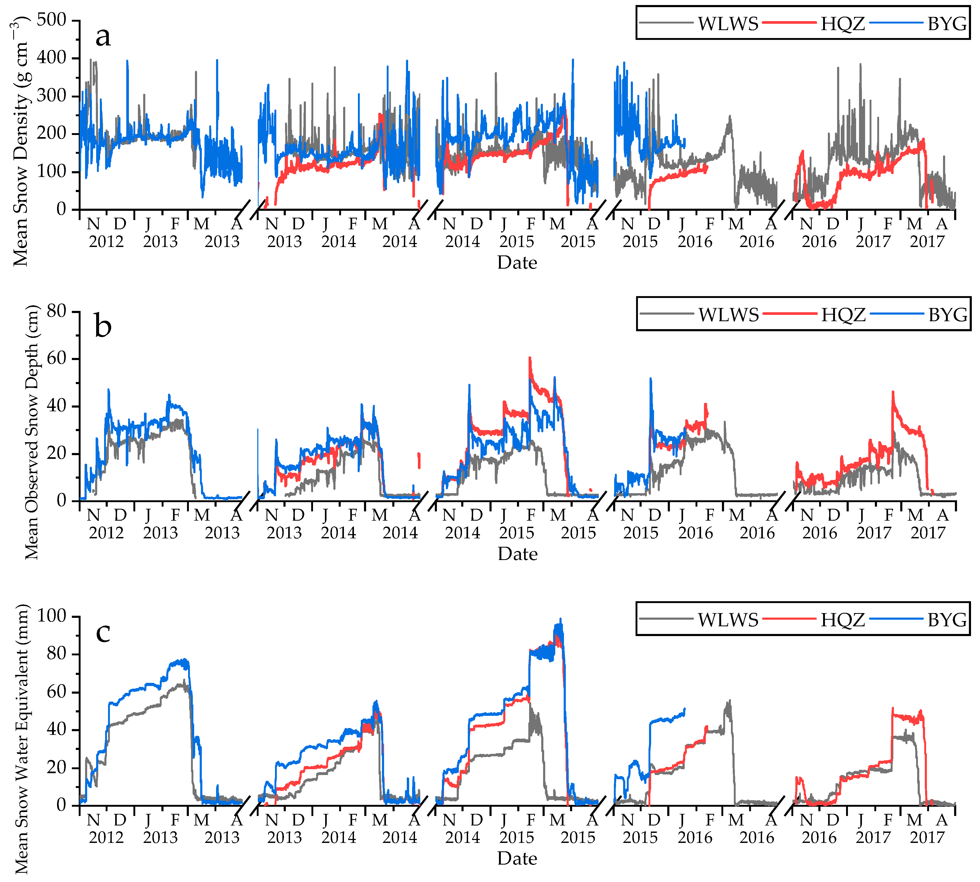
4.1. Temporal Features of the Snow Observation Data

Figure 2 shows the observed interannual and seasonal variability of the snow depth, SWE, and snow density at WLWS, HQZ, and BYG during the five snow accumulation periods from 1 November to 31 March of the following year between 2012 and 2017. However, there are missing values for the BYG site after January 2016. Additionally, some values are missing from the HQZ site in February 2016 and in the winter season of 2012–2013 (November–March).

As shown in Figure 2, after the snowfall occurred in the three regions at the beginning of November within one snow accumulation year, the snow depth and SWE increased in a step-like manner, indicating that the changes in the snow variables were not gradual and consistent increases. When there was a snowfall event or temperature increase, the increases or decreases were significant, and the data before and after the process showed a steep increase or decrease. The maximum snow depth occurred in February. Subsequently, the snow depth decreased rapidly, and the snowmelt was mostly completed by the end of March, although noticeable seasonal variations occurred. The snowmelt was accompanied by decreases in snow depth and SWE. Variations in the snow depth occurred continuously under the joint action of snow cover and external meteorological factors. Differences in the melting time and melting ratios were present on short time scales. The rapid decrease in the snow depth did not influence the variations in SWE, and snowmelt occurred during different time periods, even in winter, which demonstrated the snow accumulation features in an arid environment.

From the first snowfall to snow melting and disappearance within a single snow accumulation year, the snow density in the three regions continuously changed. Without new snowfall and snow melting, the density continuously increased under the action of gravity. The density further increased under the actions of settling and wind. The change in snow density is the result of the continuous change in snow grain diameter caused by the densification and metamorphism of the snow cover [48]. Generally, snow has a crystalline structure, and the density of snow is low (between 50 g cm⁻³ and 120 g cm⁻³). Over time, snowflakes turn to granules. The liquid water content increases, and the density increases to 100–400 g cm⁻³. At the beginning of the annual snowfall season (in November) and the beginning of annual snowmelt (at the end of February and beginning of March), the accumulated snow density greatly fluctuated. The snow density was mostly stable between December and January of the following year, fluctuating between 200 g cm⁻³ and 300 g cm⁻³.

In different regions within the same snow accumulation year, the snowfall amount increased with increasing elevation. The spatial distribution features regarding the maximum snow depth and SWE showed the following sequence: WLWS < HQZ < BYG. Within the corresponding snow accumulation year, HQZ had the minimum snow density, whereas BYG had the maximum snow density. Within the snow accumulation periods between 2012 and 2017, the average snow depths of WLWS, HQZ, and BYG were 14.8 cm, 24.3 cm, and 21.6 cm, respectively. The average maximum snow depths were 31.1 cm, 46.0 cm, and 48.1 cm, respectively. The average SWE values were 21.8 mm, 30.1 mm, and 38.8 mm, respectively. The maximum SWE values were 54.2 mm, 59.6 mm, and 70.9 mm, respectively. The average snow densities were 151.7 g cm⁻³, 113.7 g cm⁻³, and 180.3 g cm⁻³, respectively. The average maximum snow densities were 375.9 g cm⁻³, 209.1 g cm⁻³, and 378.2 g cm⁻³, respectively.

Within different snow accumulation years in the same region, the snow variables showed noticeable interannual differences. Based on the time series of snow variables after removing outliers, the maximum and average values of snow depth, SWE and snow density from 1 November to 30 April of each year from 2012 to 2017 at the three stations were calculated. The statistical results were as follows. WLWS showed maximum snow depth and SWE values within the 2012–2013 snow accumulation year during the investigation, with maximum values of 34.6 mm and 66.86 mm, respectively. HQZ and BYG showed maximum snow depth and SWE values within the 2014–2015 snow accumulation year during the investigation, with maximum values of 60.57 mm and 92.38 mm at HQZ, respectively, and 52.51 mm and 99.13 mm at BYG, respectively. The average snow density at WLWS, HQZ, and BYG from 2012–2017 were 147.4 g cm⁻³, 117.7 g cm⁻³, and 180.2 g cm⁻³, respectively.

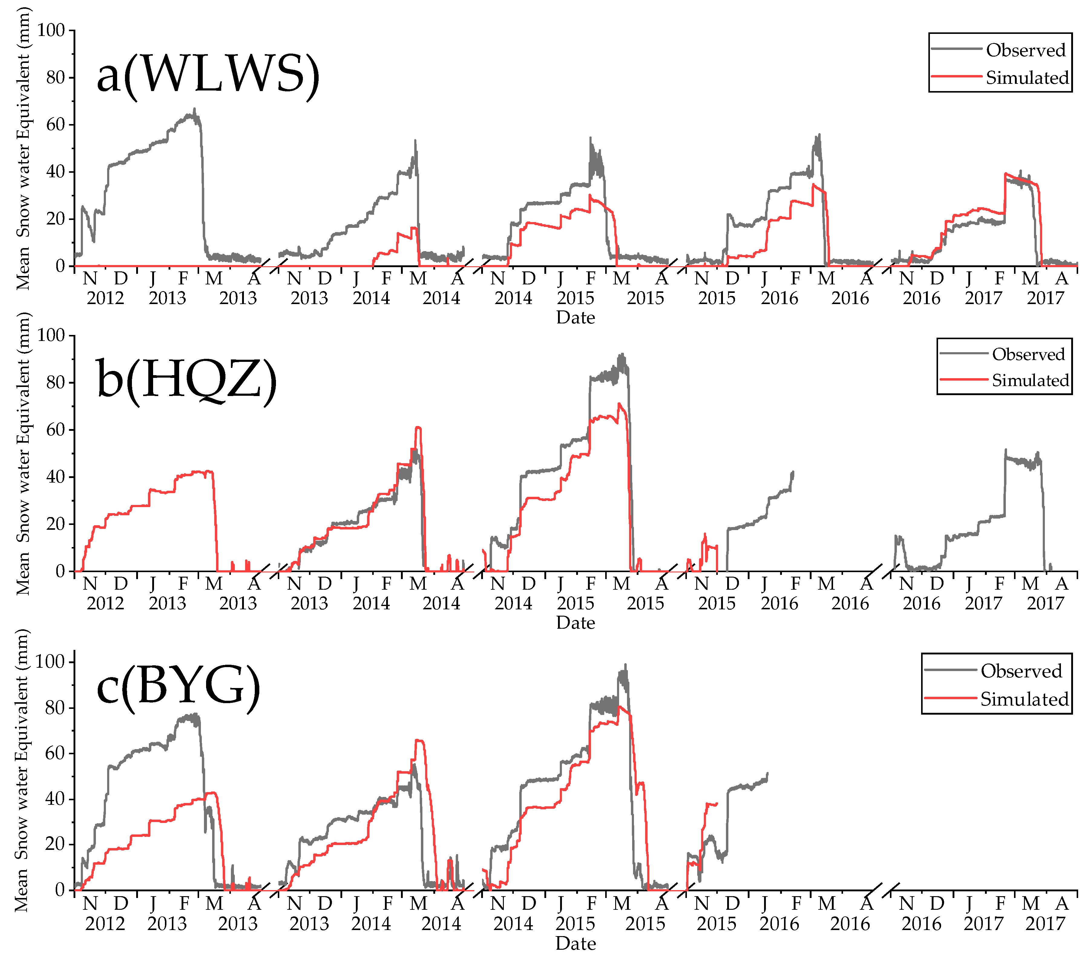
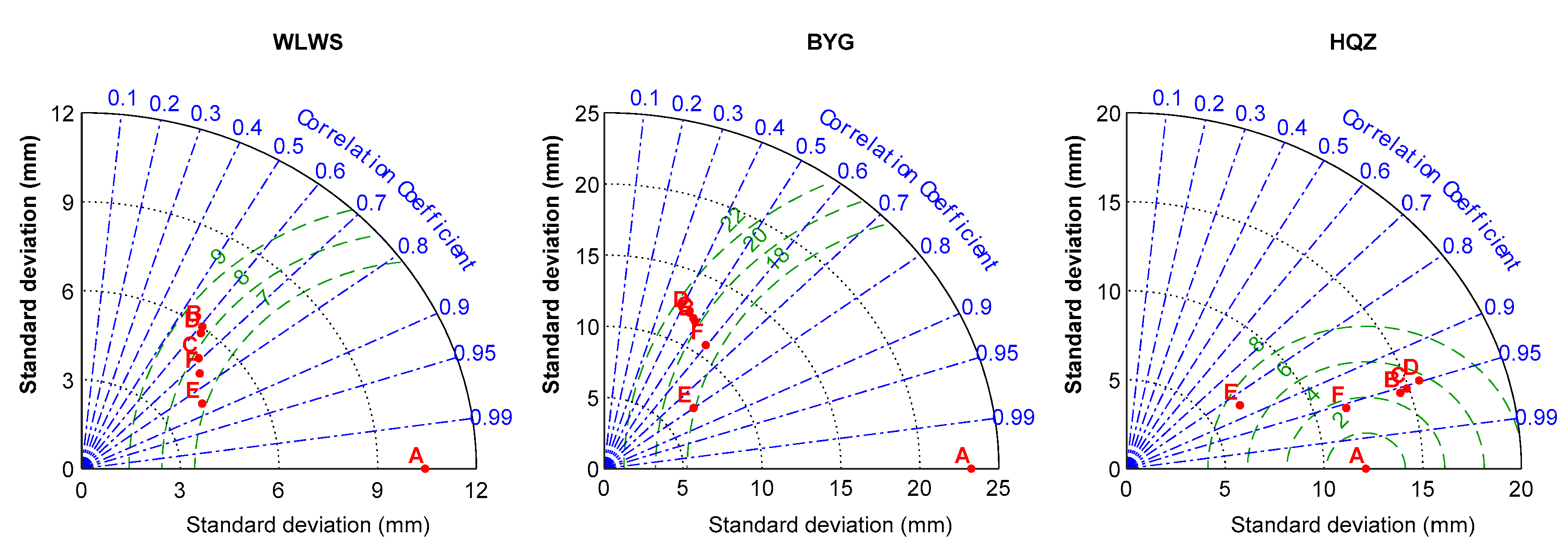
4.2. Simulated SWE Evaluation

4.2.1. Simulated SWE Evaluation

Figure 3 shows the comparative outcomes of SWE (red line) simulated by the UEB model and SWE (black line) measured by snow pillow measurements. As shown in Figure 3, unlike the measured value, the simulation was somewhat delayed, showing postponed melting. The simulated values were generally lower than the measured values during the snow accumulation period, and a general lag phenomenon was observed during the snowmelt period (examples can be found at WLWS and HQZ during the 2014–2015 snow accumulation year). The reason for this phenomenon may be explained as follows. In the snow melting stage, the liquid water content increases, resulting in a noticeable increase in the snow density, whereas the density variations in the parameterization protocol of the model were slow. However, the trend based on the simulation experiment was consistent with that based on the observations, which indicates that snow melting demonstrated remarkable seasonal variations and interannual differences.

The average SWE of the five snow accumulation years (2012–2017) obtained from snow pillow measurements and simulations are summarized in

Table 4. Model error statistics at the three automatic snow stations.

Station/Season	1 November 2012–30 April 2013	1 November 2013–30 April 2014	1 November 2014–30 April 2015	1 November 2015–30 April 2016	1 November 2016–30 April 2017
RMSE
WLWS	/	/	9.24	10.56	5.866
HQZ	/	5.186	12.9	/	/
BYG	27.59	13.4	21.64	/	/
RSR
WLWS	/	/	0.626	0.663	0.480
HQZ	/	0.3024	0.396	/	/
BYG	0.249	0.921	0.706	/	/
NSE
WLWS	/	/	0.607	0.559	0.769
HQZ	/	0.908	0.843	/	/
BYG	0.937	0.140	0.501	/	/

. In the table, “/” indicates missing data. With regard to the NSE, except for the minimum NSE coefficient of BYG during the 2013–2014 snow accumulation year (NSE = 0.140; “unsatisfactory”), the coefficients of the three regions were all higher than 0.5 (most were higher than 0.6, which indicates “excellent”). These results indicate that the UEB-simulated SWE agreed with the measured data and that the UEB model possessed a satisfactory capacity to simulate the snow accumulation process. For the RSR index, the simulated outcomes during the three snow accumulation years at WLWS were “satisfactory”, and those at HQZ during two snow accumulation years were considered “very excellent”. However, the simulated outcomes at BYG during the three snow accumulation years varied greatly, with one being “very excellent” and two being “unsatisfactory”. The RMSE values were low at WLWS and HQZ (approximately 10 mm), whereas they were high at BYG, which featured the highest actual SWE value in this region. Based on the NSE, RMSE, and RSR indexes, the SWE simulation accuracy varied greatly among the years as well as among the stations. For instance, the simulated values for WLWS in the snowmelt periods of 2014 and 2015 were lower than the measured values, but the degree of agreement between the simulated peak and measured peak was moderate, which accounted for 61% of the maximum measured peak value. Comparisons among stations and years showed that the model could reasonably predict the SWE and snow melting processes at these stations.

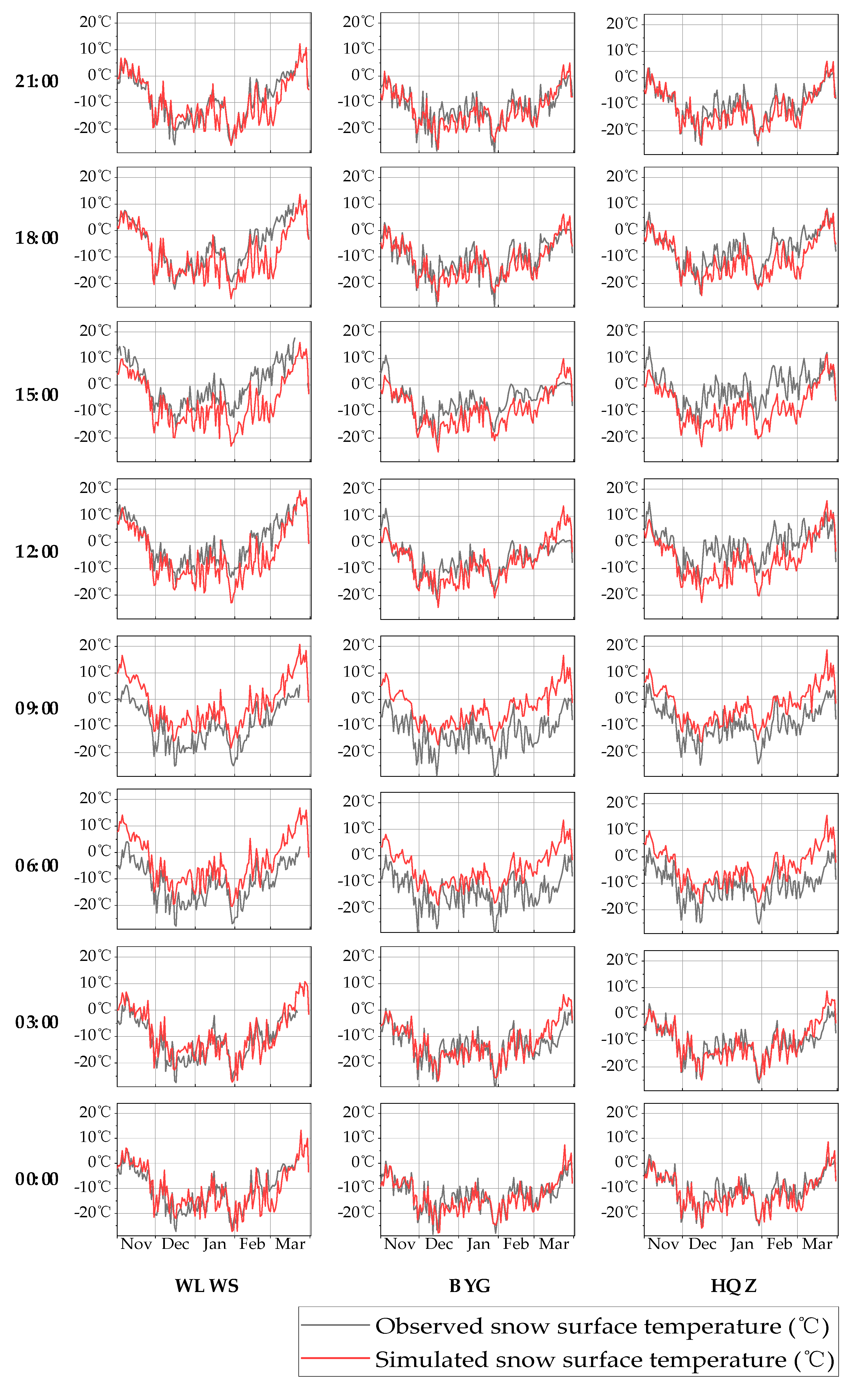
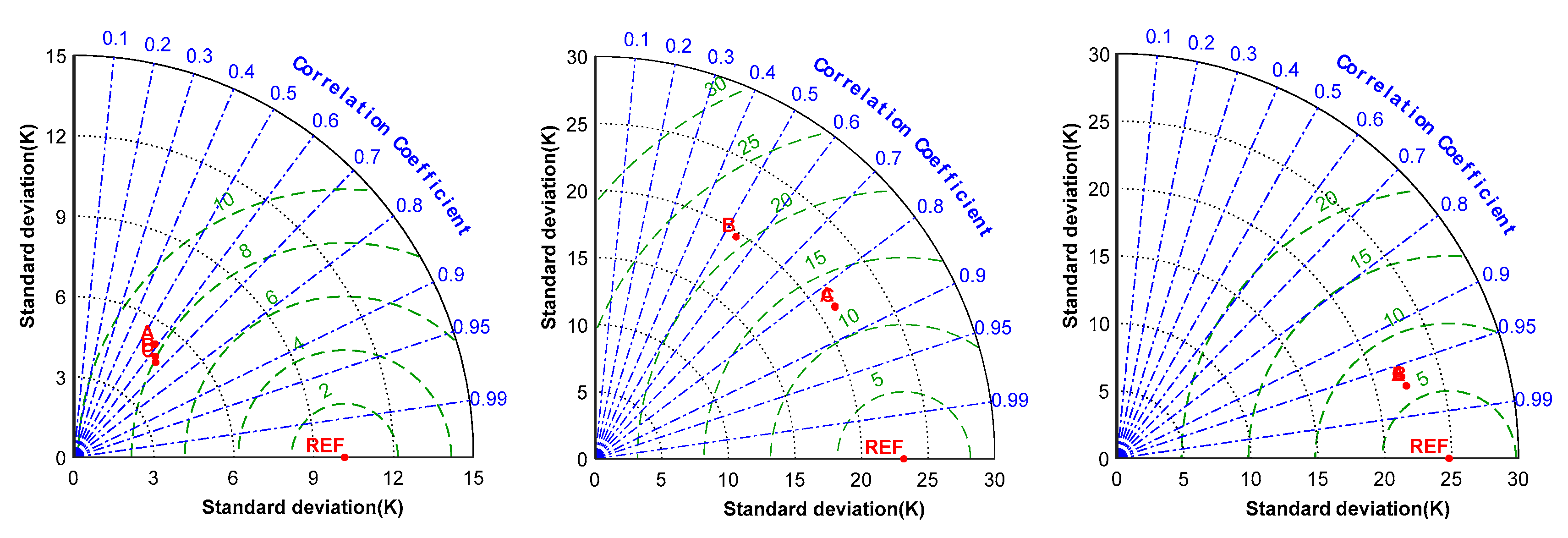
4.2.2. Snow Surface Temperature

The UEB model calculates the snow surface temperature by balancing the energy flux of the snow surface [32]. The agreement between the temperature simulated by the UEB model and the measured data indicates that the surface energy flux model is satisfactorily established and that the energy items can be used for the characteristic analysis. Although we ran a five-year simulation from 1 October 2012 to 30 September 2017 at the 3-h step, only the period between 1 November 2014 and 31 March 2015 features complete time series from all the measuring devices. However, W (m), U (kJ m⁻²), and the age of the snow surface are unknown due to the lack of observation equipment. Thus, these three model energy variables are assumed to be zero when modeling. These assumptions will inevitably lead to errors at the beginning of the simulation. However, the errors diminish with time as the model adjusts to the driving inputs. Therefore, it is most meaningful to interpret the results after these initial errors have been reduced. The time period between 1 November 2014 and 31 March 2015 was selected (the observed data were complete for the three stations during this period) because the model achieved good results during that time and analysis of the energy flux variability is feasible and credible. The simulated outcomes were used for the energy variable analysis during the 2014–2015 snow accumulation year. During this period, the total precipitation amount at WLWS was 87.6 mm, which was all snow, with an average air temperature of −6.49 °C and an average wind speed of 1.17 m·s⁻¹. The total precipitation amount at HQZ was 151.91 mm, which was all snow, with an average air temperature of −8.01 °C and an average wind speed of 1.62 m·s⁻¹. The total precipitation amount at BYG was 141.92 mm, which was all snow, with an average air temperature of −9.28 °C and an average wind speed of 1.78 m·s⁻¹.

Figure 4 shows the scatter diagrams and time series of the 3-h average measured and simulated snow surface temperature at WLWS, HQZ, and BYG. As shown in the scatter diagrams of Figure 4 (left), the simulated 3-h average snow surface temperatures in the three stations all perform well against the observed snow temperature variable with mean absolute error (MAE) values between 4.69 and 5.40 °C and RMSE values between 6.09 and 6.79 °C. The fitting outcomes of the scatter diagrams show that the correlation coefficients between the measured data and simulated data at WLWS, HQZ, and BYG were 0.71, 0.67, and 0.69, respectively. The values of the three evaluation indexes RMSE, MAE, and R quantitatively show that the degree of agreement between the measured data and simulated data was satisfactory. Figure 5 shows the time series of the measured and simulated data at WLWS, HQZ, and BYG at different time points. The simulation accuracies at 0:00, 3:00, and 6:00 were all satisfactory for the three regions. Although a low simulation accuracy was observed at HQZ for 15:00 and 18:00, the correlation coefficients were both approximately 0.6. The correlation coefficients at BYG for 6:00 and 9:00 were approximately 0.7, and the linear fitting coefficients at WLWS for all time points were greater than 0.9 (

Table 5. The correlation coefficients between the measured snow surface temperature and simulated values at different time points.

Stations/Time	0:00	3:00	6:00	9:00	12:00	15:00	18:00	21:00	ALL
WLWS	0.973	0.972	0.969	0.962	0.948	0.943	0.940	0.922	0.910
HQZ	0.883	0.880	0.860	0.822	0.836	0.603	0.690	0.874	0.654
BYG	0.840	0.819	0.747	0.778	0.842	0.822	0.856	0.840	0.745

).

4.2.3. Energy Flux Variability Related to Snow Accumulation and Melt Processes

Figure 6 and Figure 7 show the time series of energy variables of WLWS, HQZ, and BYG during the 2014–2015 snow accumulation year. As shown in Figure 6 and Figure 7, the local-scale net radiation, absolute sensible heat fluxes and latent heat fluxes, and the sum of energy fluxes into/out of snow for the three typical underlying surfaces during the accumulation period were all noticeably lower than those during the melting period. The snow net radiation presented noticeable daily variations, and the values were positive during the daytime and negative during the nighttime. Thus, the snow absorbed radiation energy while melting in the daytime and released energy while cooling and freezing at night. Net radiation serves as the primary energy source for snow melting. In this study, the contributions of net radiation to different regions formed the following order: piedmont clinoplain < mountain forest vegetation belt < mountain dessert grassland belt, with contribution percentages of 75%, 86%, and 88%, respectively (

Table 6. Contribution percentages (%) of the net radiation and net turbulence flux to snow mass loss during the snow accumulation period.

		Month	WLWS		BYG		HQZ
			Qe + Qh	NetRad	Qe + Qh	NetRad	Qe + Qh	NetRad
Snow Accumulation period	Accumulation stage	November	39.94	60.06	50.82	49.18	40.91	59.09
		December	49.39	50.61	49.97	50.03	47.88	52.12
		January	51.12	48.88	54.89	45.11	53.03	46.97
		February	48.83	51.17	44.31	55.69	48.76	51.24
	Melting stage	March	24.99	75.01	13.55	86.45	11.89	88.11

).

As shown in Figure 7, the variation in the turbulence flux was manifested by similar fluctuations with comparable magnitudes but opposite directions in the latent and sensible heat fluxes. The higher the wind speed was, the higher the absolute values of latent and sensible heat fluxes. During the melting stage, the sensible heat fluxes were positive, and the latent heat fluxes were negative. During the melting process, net radiation is the most important energy source for snow cover, and latent heat is the primary energy source for sublimation and evaporation of snow cover. According to the contribution percentages of net turbulence, the different regions were ordered as follows: piedmont clinoplain > mountain forest vegetation belt > mountain desert grassland belt (with percentages of 25%, 14%, and 12% at WLWS, BYG, and HQZ, respectively (Table 6).

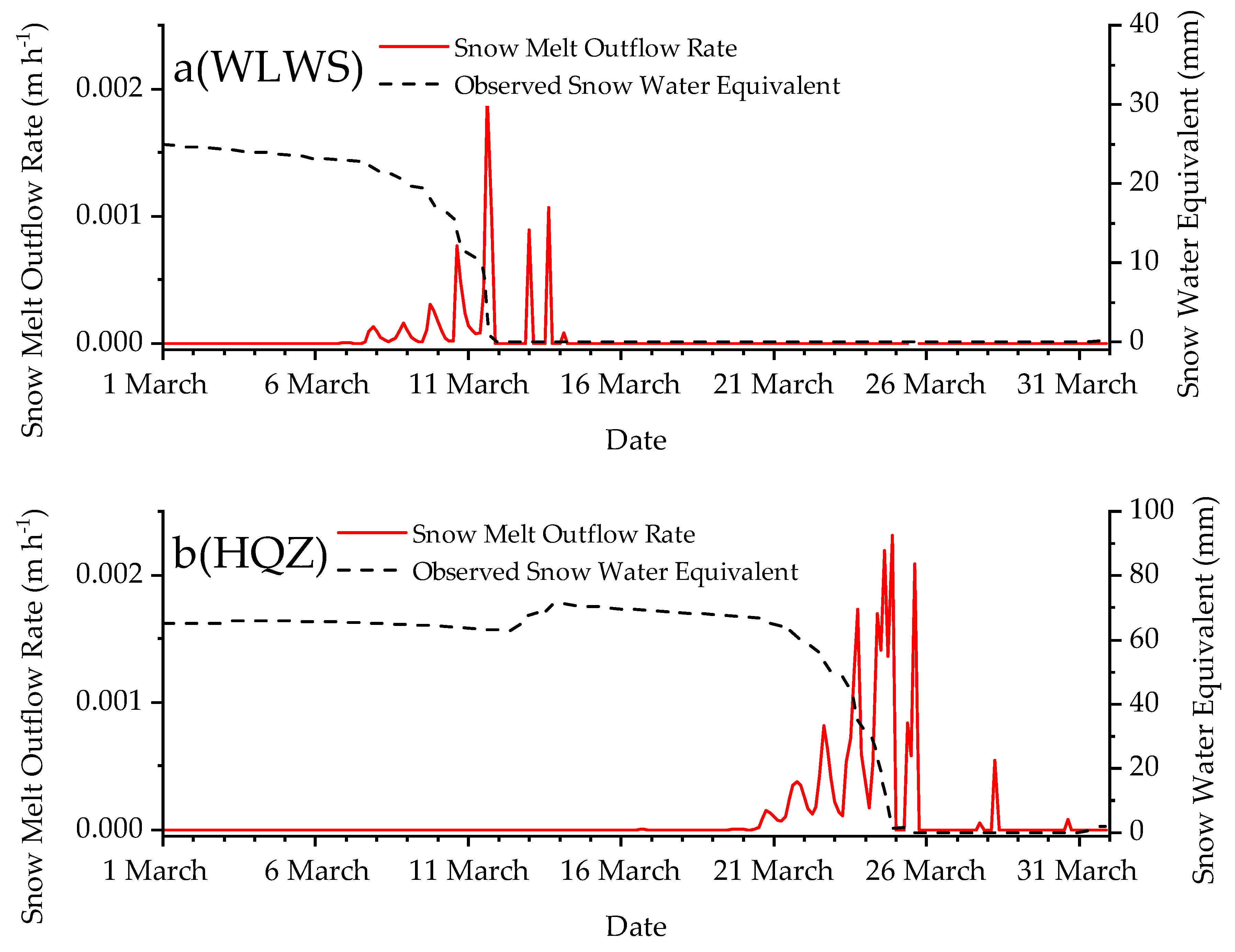
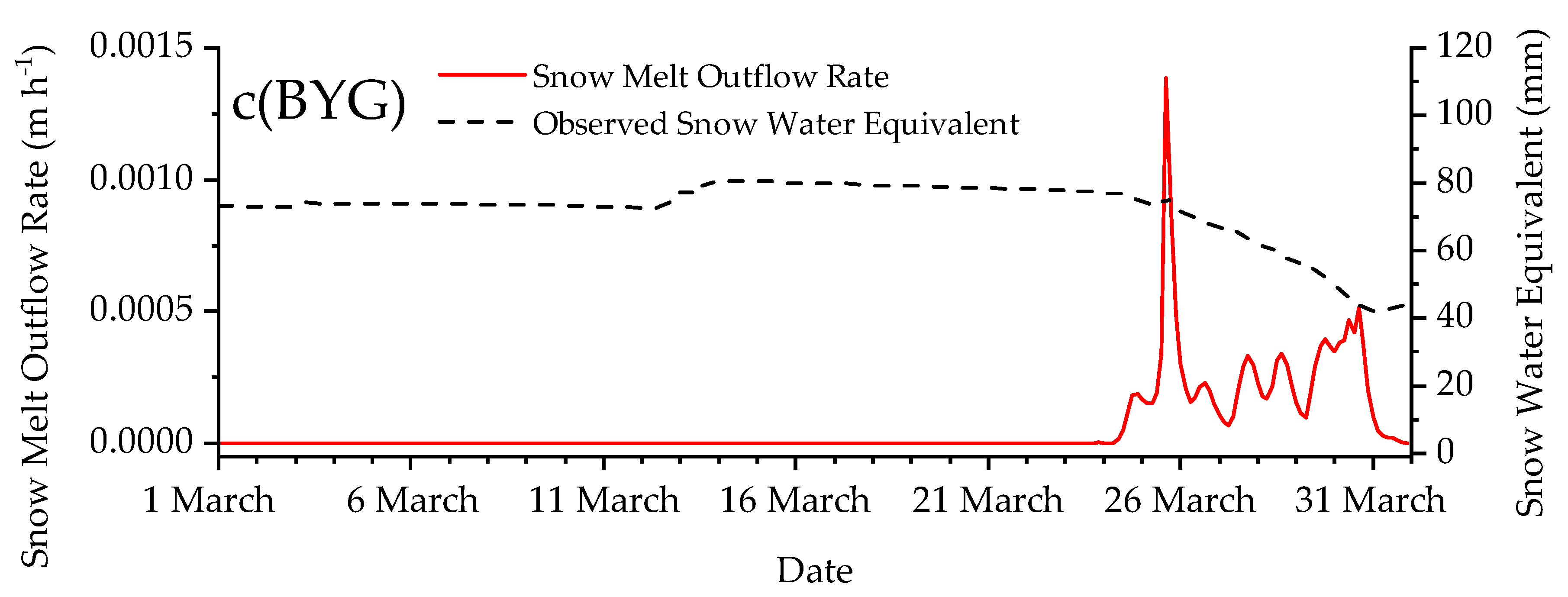
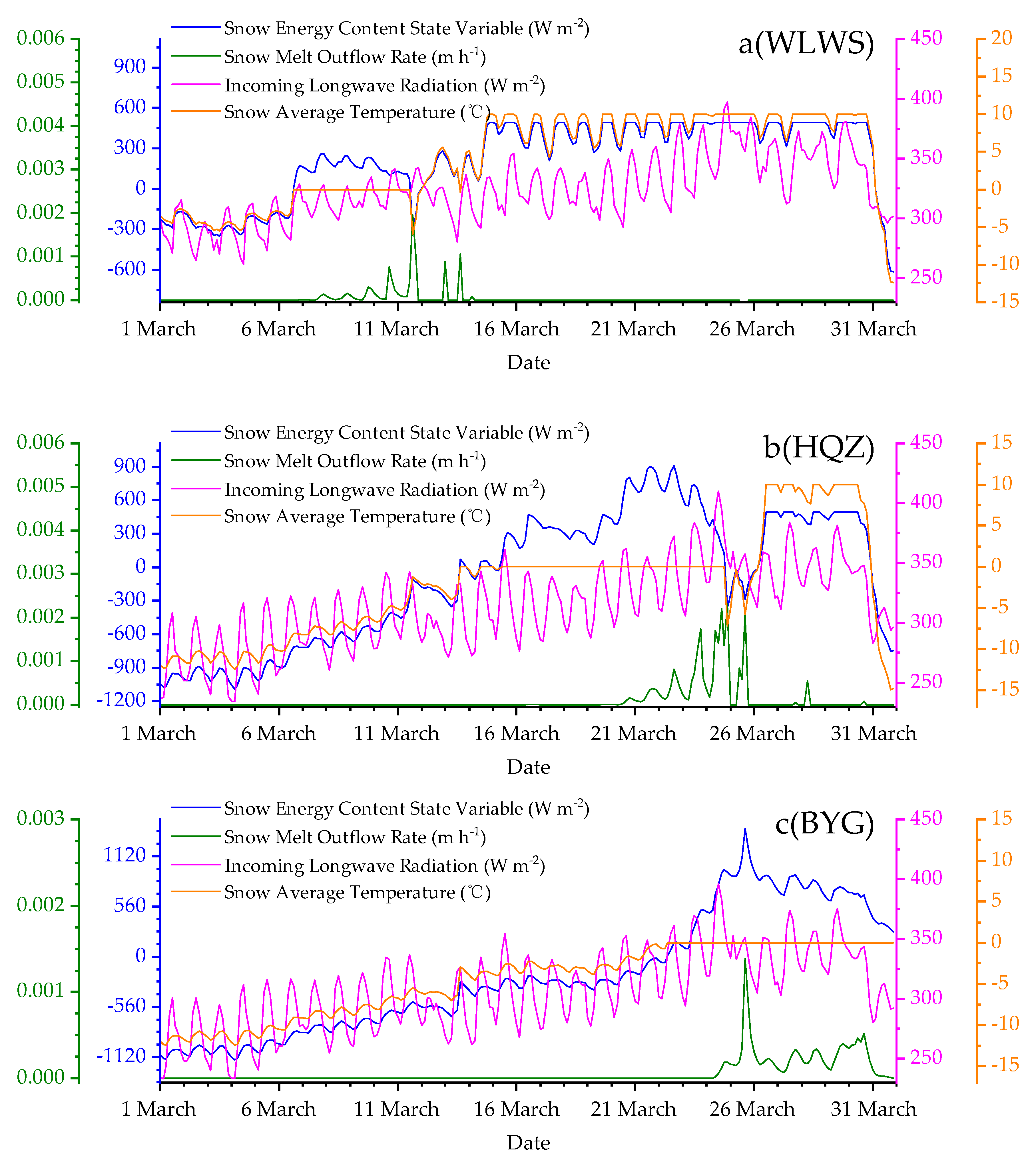
4.2.4. Characteristics of Longwave Radiation, Energy Content, and Snowmelt Outflow

The snowmelt amount and air temperature are the factors most associated with the snowmelt outflow rate (m/h). The rate showed a strong relationship with the increase in SWE, particularly during the stage where SWE noticeably decreased (Figure 8). Incoming longwave radiation led to a change in the average snow temperature because of an increase in the snow energy content, which promoted snow melting, and only a small portion of the input energy was used for snow runoff generation [49]. The snow cover receives continuous energy, which leads to the production of liquid water. Liquid water is bound within gaps in the snow crystals under the action of capillary forces. When the amount of liquid water overcomes the effect of capillary forces, the water migrates downward due to gravity, and the snowmelt water flows out of the snowpack. The net heat exchanged between the air and snow is positive. When the snow surface temperature reaches 0 °C, the surplus heat causes snowmelt. At this point, the snow temperature no longer increases (Figure 9).

To validate the accuracy of the outflow model, the water balance in March was calculated in this study. According to the mass conservation principle, the snow outflow and sublimation amount should increase with the decrease in the snow amount. When snowfall occurs, the amount of snow increases. In this study, the snow outflow and sublimation amounts were defined as the amount of loss during the snowmelt process, and the initial SWE and precipitation were defined as the original water amount. WLWS was taken as an example. According to the observed data, the initial SWE of the snow melting process was 0.02289 m, and the precipitation was 0.01500 m. The modeled snowmelt outflow loss was 0.03556 m, and the sublimation loss was 0.00436 m, with a total modeled loss of 0.03992 m. The modeled loss agreed with the measured loss (0.03789 m), which indicates that the water content remained balanced during model establishment and that the outflow model was reliable (

Table 7. Comparison between the simulated water loss and measured water loss in March 2015.

Stations		BYG	HQZ	WLWS
Obtained water	Initial SWE (m)	0.08460	0.08468	0.02289
	Precipitation (m)	0.00771	0.00857	0.01500
	Sum of these two terms (m)	0.09231	0.09325	0.03789
Lost water	Sublimation (m)	0.015402	0.015024	0.00436
	Melt (m/h)	0.074499	0.073759	0.03556
	Sum of these two terms (m)	0.089901	0.088783	0.03992

).

4.2.5. Evaporation and the Difference among the Three Stations

The local-scale average monthly air temperatures in the piedmont clinoplain (WLWS), mountain desert grassland belt (HQZ), and mountain forest vegetation belt (BYG) between November 2014 and February 2015 were below 0 °C. During this time, even in winter, several melting periods occurred (Figure 10), which is the typical feature of snow melting in arid environments. In the piedmont clinoplain (WLWS), the first melting period occurred on 9 November, which was due to an increase in air temperature (from 1 to 8 °C) and an increase in wind speed (from 1.4 m·s⁻¹ to 6 m·s⁻¹). The second melting period appeared on November 16, which was followed by the third melting period on 26 November. In the mountain desert grassland belt (HQZ), the first melting period occurred on 4 November, followed by the second on 9 November and the third on 24 November. In the mountain forest vegetation belt (BYG), the first melting period occurred on 5 November, followed by the third on 8 November and the fourth on 24 March. Sublimation was noticeably higher during the melting stage than during the accumulation stage. At WLWS, the snowmelt amount was 68 mm, and the sublimation amount was 20 mm. At HQZ, the snowmelt amount was 115 mm, and the sublimation amount was 38 mm. At BYG, the snowmelt amount was 74 mm, and the sublimation amount was 24 mm. The wind speed and solar radiation strength increased with increasing elevation. In the area higher than 1000 m above sea level, the effect of sublimation may be more important (

Table 8. Different energy component contributions to snow mass loss.

			Cumulative Precipitation from the Beginning of the Model Run (mm)			Cumulative Sublimation from the Beginning of the Model Run (mm)			Cumulative Melt Outflow from the Beginning of the Model Run (mm)
		Time/Stations	HQZ	BYG	WLWS	HQZ	BYG	WLWS	HQZ	BYG	WLWS
Snow accumulation period	Accumulation stage	November	65.78	57.80	40.80	10.18	9.17	2.64	41.09	30.15	28.90
		December	83.67	76.49	52.20	12.32	10.28	6.07	41.09	30.15	28.90
		January	107.25	97.86	62.40	17.46	12.64	9.30	41.09	30.15	28.90
		February	129.08	118.67	72.60	22.80	15.39	15.72	41.09	30.15	31.96
	Melting stage	March	154.91	141.92	87.60	37.82	23.68	20.08	114.85	74.40	67.52
		Time/Stations	Wind Speed (m·s−1)			Incoming Solar Radiation (W m−2)			Temperature (°C)
			HQZ	BYG	WLWS	HQZ	BYG	WLWS	HQZ	BYG	WLWS
Snow accumulation period	Accumulation stage	November	1.73	1.90	1.39	84.11	81.56	86.31	−2.86	−4.59	−0.20
		December	1.15	1.33	0.88	70.72	69.25	69.14	−14.11	−15.49	−13.96
		January	1.70	1.89	1.39	83.97	81.47	86.14	−11.84	−13.14	−11.44
		February	1.68	1.78	1.10	75.39	74.33	75.50	−10.46	−11.07	−9.06
	Melting stage	March	2.26	2.43	1.65	87.19	85.17	89.92	−0.86	−2.14	2.15

).

5. Discussion on Model Sensitivity

First, we performed a preliminary simulation with the reference model parameters of Tarboton et al. [27] and Wu et al. [32] and found that the parameters of temperature and roughness (z_os) were relatively sensitive. Then, we evaluated these parameters individually and obtained the optimal parameters according to the Taylor diagram criteria [50,51,52,53]. By setting all parameters but one to fixed values and setting one parameter to different thresholds, the Taylor diagram provides a visual representation of the normalized standard deviation (NSD), normalized centered root mean square error (CRMS) and correlation (C) to quantify the correspondence between the observed and modeled variables. Finally, all the optimal parameters with relatively low CRMS and high C and NSD values were used for modeling, and the simulations were evaluated using the NAE, RMSE, and RSR evaluation indexes. Through a large number of experiments, we obtained the model parameters shown in Table 3.

The Taylor diagrams in Figure 11 summarize model performance at each site when all parameters but z_os are fixed and z_os is set to different thresholds. Each point (red dot) on the polar-style graph represents three statistics: NSD (black curved); normalized CRMS (Equation (6), dotted green line); and C (dotted blue line) between the observed and modeled values.

$$\mathrm{CRMS}=\frac{\sqrt{{\displaystyle \sum _{t=1}^n\left(ob{s}_t-ob{s}_{mean}\right)-\left(Si{m}_t-Si{m}_{mean}\right)}}}{n},$$

(6)

where $ob{s}_t$ and $Si{m}_t$ denote the observed and simulated values at time point t, respectively; n is the total number of time steps; and $ob{s}_{mean}$ and $Si{m}_{mean}$ are the average of the observed and simulated values, respectively.

The correspondences between the letters in the diagrams in Figure 11 and the simulated SWE values are as follows: B, SWEz_os = 0.0009 m; C, SWEz_os = 0.0005 m; D, SWEz_os = 0.001 m; E, SWEz_os = 0.05 m; and F, SWEz_os = 0.01 m. As shown in the diagrams in Figure 11, z_os had a great impact on the simulated SWE value, and the simulated SWE varied greatly according to different z_os thresholds. A threshold closer to the letter A (measured data) resulted in more satisfactory simulated SWE. When 0.01 m was taken as the z_os (point F in Figure 11), the simulated SWE was the most consistent with the measured SWE. When z_os = 0.05 m, the correlation is usually higher than 0.8, the normalized CRMS is lower than 8 and the modeled standard deviation is lower than the observed standard deviation at most sites.

Unlike z_os, the air temperature above which all precipitation is rain (Tr) had a different impact on the simulated SWE at the three sites. Except for WLWS in Figure 12 left, the model’s performance for Tr varies widely when the Tr threshold is 3, 1.2, and 0.3 °C at BYG in Figure 12 middle and HQZ in Figure 12 right, corresponding to B, C, and D in the graph. A majority of sites show a correlation of 0.6 or higher with the observations. However, an NSD less than the value of A in the diagrams indicates underdispersion of SWE compared to observed values for the three sites. Additionally, a low normalized CRMS indicates higher precision of the model for SWE.

6. Conclusions

In this study, the characteristics of the local-scale snow depth, SWE, snow surface temperature and snow density in the piedmont clinoplain, mountain desert grassland belt, and mountain forest vegetation belt of the semiarid Manas River Basin were analyzed using the snow variable measurement system. Additionally, the local-scale snow accumulation and melting processes in the three typical underlying surfaces were simulated using the UEB model. We investigated the skill and utility of the UEB model in terms of its ability to model snow accumulation and ablation, and we also obtained local model parameters, which may be directly applied in regional simulations. The main findings of this study are as follows.

• On the local scale, the variations in snow depth, SWE, and snow density in the piedmont clinoplain, mountain desert grassland belt, and mountain forest vegetation belt show similarities as well as differences. The snow variables in the three typical underlying surfaces above present noticeable seasonal and interannual characteristics. Within a single snow accumulation year, snow depth increases with increasing elevation, and multiple snow melting events occur and are primarily driven by air temperature, a typical feature of snow melting in arid environments. In terms of snow depth, the three typical underlying surfaces exhibit the following order: piedmont clinoplain < mountain desert grassland belt < mountain forest vegetation belt.
• The UEB model is a simple but useful model with only a few data requirements and no (or minimal) calibration and uses a limited number of state variables, which is convenient for spatial applications. Similar to the studies of Tarboton and Luce [26] and Wu et al. [32], our analysis also found that the model is highly sensitive to the air temperature above which all precipitation is rain (Tr) and the surface aerodynamic roughness (z_os), thus, these parameters should be modified when applying the model in different regions. However, at the local catchment scale of the Manas River Basin, consistent parameters were applied to the selected three typical underlying surfaces to model the snow ablation process, and the simulation results were demonstrated to be accurate. Moreover, the UEB model requires incoming radiation fluxes and wind speed, which are not measured at all weather stations, especially those in high-elevation, rugged terrain. Therefore, the sparse meteorological data in the area motivated the development of a methodology for driving the UEB model using globally (especially regionally) available reanalysis data.
• According to the simulation accumulation and ablation results during the 2012–2017 snow accumulation years, the minimum NSE values for WLWS, HQZ, and BYG were 0.645, 0.8755, and 0.526, respectively, and the predicted SWE values were mostly consistent with the measured values, indicating that the model could reasonably simulate SWE evolution characteristics in the selected three typical underlying surfaces. The correlation coefficients between the measured snow surface temperature and simulated outcomes at WLWS, HQZ, and BYG were 0.71, 0.67, and 0.69, respectively, and the energy parameter could be used for the characteristic analysis of the surface energy budgets. The net radiation served as the main energy source for the melting of snow layers. The net radiation contribution percentages for WLWS, HQZ, and BYG were 75%, 86%, and 88%, and the net turbulence contribution percentages for the three observed locations were 25%, 14%, and 12%, respectively. The net radiation contribution to snow melting differed regionally from that of the net turbulence: the lowest contribution of the net radiation occurred in the piedmont clinoplain, followed by the mountain desert grassland belt and mountain forest belt, whereas the order for the net turbulence was the opposite.

References

1. Zhang, P.; Li, X.; Liu, Y.; Li, Y. Influence of winter climate on spring snowmelt runoff in Manas river basin. In Proceedings of the Annual Meeting of Chinese Meteorological Society, Beijing, China, 9–11 November 2011. [Google Scholar]
2. Zhang, P.; Wang, J.; Liu, Y.; Li, Y. Application of SRM to Flood Forecast and Forwarning of Manasi River Basin in Spring. Remote Sens. Technol. Appl. 2009, 24, 456–461. [Google Scholar] [CrossRef]
3. Bai, L.; Guo, L.P.; Ma, J.; Li, L.H. Observation and Analysis of the Process of Snowmelting at Tianshan Station Using the Images by Digital Camera. Resour. Sci. 2012, 34, 620–628. [Google Scholar]
4. Qiu, J.Q.; Yan, X. Study on spring snowmelt flood and its causes in the middle of north slope of Tangshan mountain. Arid Land Geogr. 1994, 3, 35–42. [Google Scholar] [CrossRef]
5. Wu, S.F.; Zhang, G.W. Preliminary Approach on the Floods and Their Calamity Changing Tendency in Xinjiang Region. J. Glaciol. Geocryol. 2003, 25, 199–203. [Google Scholar] [CrossRef]
6. Chen, X.; Bao, A.; Zhang, H.; Liu, M. A Study on Methods and Accuracy Assessment for Extracting Snow Covered Areas from MODIS Images Based on Pixel Unmixing: A Case on the Middle of the Tianshan Mountain. Resour. Sci. 2010, 32, 1761–1768. [Google Scholar]
7. Dou, Y.; Chen, X.; Bao, A.; Li, L. Study of the Temporal and Spatial Distribute of the Snow Cover in the Tianshan Mountains, China. J. Glaciol. Geocryol. 2010, 32, 28–34. [Google Scholar]
8. Feng, Q.; Zhang, X.; Liang, T. Dynamic monitoring of snow cover based on MOD10A1 and AMSR-E in the north of Xinjiang Province, China. Acta Prataculturae Sin. 2009, 18, 125–133. [Google Scholar] [CrossRef]
9. Ma, X.; Liu, Z.; Xiao, J. The Comparison between NOAA satellite and MODIS in Snow Monitoring Mode. Res. Soil Water Conserv. 2008, 15, 220–222. [Google Scholar]
10. Pei, H.; Fang, S.; Qin, Z.; Liu, Z. Remote sensing based monitoring of coverage and depth of snow in northern Xinjiang. J. Nat. Disasters 2008, 17, 52–57. [Google Scholar] [CrossRef]
11. Meng, X.; Ji, X.; Sun, Z.; Kong, X.; Liu, Z. Sensitive Analysis of Snowmelt Runoff on North Slope of Tianshan Mountains—Taking Juntanghu Watershed as an Example. Bull. Soil Water Conserv. 2014, 34, 277–282. [Google Scholar] [CrossRef]
12. Feng, X.; Li, W.; Shi, Z.; Wang, L. Satellite Snowcover Monitoring and Snowmelt Runoff Simulation of Manas River in Tianshan Region. Remote Sens. Technol. Appl. 2000, 15, 18–21. [Google Scholar] [CrossRef]
13. Li, B.; Zhang, Y.; Zhou, C. Snow Cover Depletion Curve in Kaidu River Basin, Tianshan Mountains. Resour. Sci. 2004, 26, 23–29. [Google Scholar] [CrossRef]
14. Singh, P.; Kumar, N.; Arora, M. Degree-day factors for snow and ice for Dokriani Glacier, Garhwal Himalayas. J. Hydrol. 2000, 235, 1–11. [Google Scholar] [CrossRef]
15. Carl, P.; Gerlinger, K.; Hattermann, F.F.; Krysanova, V.; Schilling, C.; Behrendt, H. Regularity-based functional streamflow disaggregation: 2. Extended demonstration. Water Resour. Res. 2008, 44. [Google Scholar] [CrossRef] [Green Version]
16. Besic, N.; Vasile, G.; Gottardi, F.; Gailhard, J.; Urso, G.; Besic, N.; Vasile, G.; Gottardi, F.; Gailhard, J.; Girard, A. Calibration of a distributed SWE model using MODIS snow cover maps and in situ measurements. Remote Sens. Lett. 2014, 5, 230–239. [Google Scholar] [CrossRef]
17. Boudhar, A.; Hanich, L.; Boulet, G.; Duchemin, B.; Berjamy, B.; Chehbouni, A. Evaluation of the Snowmelt Runoff model in the Moroccan High Atlas Mountains using two snow-cover estimates. Hydrol. Sci. J. 2009, 54, 1094–1113. [Google Scholar] [CrossRef]
18. Romshoo, S.A.; Rafiq, M.; Rashid, I. Spatio-temporal variation of land surface temperature and temperature lapse rate over mountainous Kashmir Himalaya. J. Mt. Sci. 2018, 15, 563–576. [Google Scholar] [CrossRef]
19. Anderson, E.A. A Point Energy and Mass Balance Model of a Snow Cover; NWS Technical Report; The National Oceanic and Atmospheric Administration: Silver Spring, MD, USA, 1976; Volume 19. [CrossRef]
20. Bartelt, P.; Lehning, M. A physical SNOWPACK model for the Swiss avalanche warning Part I: Numerical model. Cold Reg. Sci. Technol. 2002, 35, 123–145. [Google Scholar] [CrossRef]
21. Lawrence, D.M.; Oleson, K.W.; Flanner, M.G.; Thornton, P.E.; Swenson, S.C.; Lawrence, P.J.; Zeng, X.; Yang, Z.-L.; Levis, S.; Sakaguchi, K.; et al. Parameterization improvements and functional and structural advances in Version 4 of the Community Land Model. J. Adv. Model. Earth Syst. 2011, 3, M03001. [Google Scholar] [CrossRef]
22. Brown, M.E.; Racoviteanu, A.E.; Tarboton, D.G.; Gupta, A.S.; Nigro, J.; Policelli, F.; Habib, S.; Tokay, M.; Shrestha, M.S.; Bajracharya, S.; et al. An integrated modeling system for estimating glacier and snow melt driven streamflow from remote sensing and earth system data products in the himalayas. J. Hydrol. 2014, 519, 1859–1869. [Google Scholar] [CrossRef]
23. Sen Gupta, A.; Tarboton, D.G.; Racoviteanu, A.; Brown, M.; Habib, S. Estimating Snow and Glacier Melt in a Himalayan Watershed Using an Energy Balance Snow and Glacier Melt Model. In Proceedings of the AGU Fall Meeting, San Francisco, CA, USA, 15–19 December 2014. AGU Fall Meeting Abstracts. [Google Scholar]
24. Sorooshian, S.; Hsu, K.L.; Sultana, R.; Li, J. Evaluating the Utah energy balance (UEB) snow model in the noah land-surface model. Hydrol. Earth Syst. Sci. 2014, 18, 3553–3570. [Google Scholar] [CrossRef]
25. Luce, C.H.; Tarboton, D.G. Modeling Snowmelt over an Area: Modeling Subgrid Scale Heterogeneity in Distributed Model Elements. In Proceedings of the MODSIM 2001—International Congress on Modelling and Simulation, Canberra, Australia, 10–13 December 2001; pp. 341–346. [Google Scholar]
26. Tarboton, D.G.; Luce, C.H. Utah Energy Balance Snow Accumulation Melt Model (UEB), Computer Model Technical Description and Users Guide; Utah Water Research Laboratory: Logan, UT, USA; USDA Forest Service Intermountain Research Station: Fort Collins, CO, USA, 1996; 64p.
27. Tarboton, D.G. Measurement and Modeling of Snow Energy Balance and Sublimation from Snow. In Proceedings of the International Snow Science Workshop, Snowbird, UT, USA, 31 October–2 November 1994. Utah Water Research Laboratory Working Paper no. WP-94-HWRDGT/002. [Google Scholar]
28. Rutter, N.; Essery, R.; Pomeroy, J.; Altimir, N.; Andreadis, K.; Baker, I.; Barr, A.; Bartlett, P.; Boone, A.; Deng, H.; et al. Evaluation of forest snow processes models (SnowMIP2). J. Geophys. Res. Atmos. 2009, 114. [Google Scholar] [CrossRef] [Green Version]
29. Luce, C.H.; Tarboton, D.G.; Service, F.; Mountain, R. Evaluation of alternative formulae for calculation of surface temperature in snowmelt models using frequency analysis of temperature observations. Hydrol. Earth Syst. 2010, 14, 535–543. [Google Scholar] [CrossRef] [Green Version]
30. Mahat, V.; Tarboton, D.G. Canopy radiation transmission for an energy balance snowmelt model. Water Resour. Res. 2012, 48. [Google Scholar] [CrossRef] [Green Version]
31. You, J.; Tarboton, D.G.; Luce, C.H. Modeling the snow surface temperature with a one-layer energy balance snowmelt model. Hydrol. Earth Syst. Sci. 2014, 18, 5061–5076. [Google Scholar] [CrossRef] [Green Version]
32. Wu, X.; Wang, N.; Shen, Y.; He, J.; Zhang, W. In-situ observations and modeling of spring snowmelt processes in an Altay Mountains river basin. J. Appl. Remote Sens. 2014, 8, 084697. [Google Scholar] [CrossRef]
33. Gao, L.; Zhang, Y.; Shen, Y.; Zhang, L. Analysis of water and heat transfer in snow layer during snowmelt period in Irtysh River Basin based on energy balance theory. J. Glaciol. Geocryol. 2016, 38, 323–331. [Google Scholar] [CrossRef]
34. Wang, S.J.; Zhang, M.J.; Li, Z.Q. Response of glacier area variation to climate change in Chinese Tianshan Mountains in the past 50 years. Acta Geogr. Sin. 2011, 66, 38–46. [Google Scholar] [CrossRef]
35. Sun, C.; Chen, Y.; Li, W.; Li, X.; Yang, Y. Isotopic time series partitioning of streamflow components under regional climate change in the urumqi river, northwest china. Int. Assoc. Sci. Hydrol. Bull. 2015, 61, 1443–1459. [Google Scholar] [CrossRef]
36. Tang, X.L.; Xu, L.P.; Zhang, Z.Y.; Lv, X. Effects of glacier melting on socioeconomic development in the manas river basin, China. Nat. Hazards 2013, 66, 533–544. [Google Scholar] [CrossRef]
37. Chen, N.; Feng, X.Z.; Xiao, P.F.; He, G.J. AnalysisofsnowlayerparametersinManasiRiverBasin. J. Nanjing Univ. (Nat. Sci.) 2015, 51, 936–943. [Google Scholar] [CrossRef]
38. Schulz, O.; Jong, C.D. Snowmelt and sublimation: Field experiments and modelling in the high atlas mountains of morocco. Hydrol. Earth Syst. Sci. 2004, 8, 1076–1089. [Google Scholar] [CrossRef]
39. Rice, R.; Bales, R.; Painter, T.; Dozier, J. Snow water equivalent along elevation gradients in the merced and tuolumne river basins of the sierra nevada. Water Resour. Res. 2011, 47, W08515. [Google Scholar] [CrossRef]
40. Fausto, R.S.; Van As, D.; Ahlstrøm, A.P.; Citterio, M. Assessing the accuracy of greenland ice sheet ice ablation measurements by pressure transducer. J. Glaciol. 2012, 58, 1144–1150. [Google Scholar] [CrossRef]
41. Tan, J.; Yang, L.; Grimmond, C.S.B.; Shi, J.; Gu, W.; Chang, Y.; Hu, P.; Sun, J.; Ao, X.; Han, Z. Urban integrated meteorological observations: Practice and experience in Shanghai, China. Bull. Am. Meteorol. Soc. 2015, 96, 85–102. [Google Scholar] [CrossRef]
42. Avanzi, F.; De Michele, C.; Ghezzi, A.; Jommi, C.; Pepe, M. A processing-modeling routine to use SNOTEL hourly data in snowpack dynamic models. Adv. Water Resour. 2014, 73, 16–29. [Google Scholar] [CrossRef]
43. Yang, K.; He, J.; Tang, W.; Qin, J.; Cheng, C.C.K. On downward shortwave and longwave radiations over high altitude regions: Observation and modeling in the Tibetan plateau. Agric. For. Meteorol. 2010, 150, 38–46. [Google Scholar] [CrossRef]
44. Chen, Y.; Yang, K.; He, J.; Qin, J.; Shi, J.; Du, J.; He, Q. Improving land surface temperature modeling for dry land of China. J. Geophys. Res. Atmos. 2011, 116. [Google Scholar] [CrossRef]
45. Andreadis, K.M.; Lettenmaier, D.P. Assimilating remotely sensed snow observations into a macroscale hydrology model. Adv. Water Resour. 2006, 29, 872–886. [Google Scholar] [CrossRef]
46. Gupta, H.V.; Sorooshian, S.; Yapo, P.O. Status of Automatic Calibration for Hydrologic Models: Comparison with Multilevel Expert Calibration. J. Hydrol. Eng. 1999, 4, 135–143. [Google Scholar] [CrossRef]
47. Moriasi, D.N.; Arnold, J.G.; Van Liew, M.W.; Bingner, R.L.; Harmel, R.D.; Veith, T.L. Model Evaluation Guidelines for Systematic Quantification of Accuracy in Watershed Simulations. Trans. ASABE 2007, 50, 885–900. [Google Scholar] [CrossRef]
48. Lu, H.; Wei, W.; Liu, M.; Gao, P.; Han, Q. Densification and Accumulation Rate of Snow in the Stable Snow Cover Period in the Tianshan Mountains. J. Glaciol. Geocryol. 2011, 33, 374–380. [Google Scholar]
49. Colbeck, S.C. An overview of seasonal snow metamorphism. Rev. Geophys. 1982. [Google Scholar] [CrossRef]
50. Taylor, K.E. Summarizing multiple aspects of model performance in a single diagram. J. Geophys. Res. Atmos. 2001, 106, 7183–7192. [Google Scholar] [CrossRef]
51. Guo, H.; Chen, S.; Bao, A.; Hu, J.; Gebregiorgis, A.S.; Xue, X.; Zhang, X. Inter-comparison of high-resolution satellite precipitation products over Central Asia. Remote Sens. 2015, 7, 7181–7211. [Google Scholar] [CrossRef]
52. Ning, S.; Wang, J.; Jin, J.; Ishidaira, H. Assessment of the Latest GPM-Era High-Resolution Satellite Precipitation Products by Comparison with Observation Gauge Data over the Chinese Mainland. Water 2016, 8, 481. [Google Scholar] [CrossRef]
53. Tang, G.; Zeng, Z.; Long, D.; Guo, X.; Yong, B.; Zhang, W.; Hong, Y. Statistical and Hydrological Comparisons between TRMM and GPM Level-3 Products over a Midlatitude Basin: Is Day-1 IMERG a Good Successor for TMPA 3B42V7? J. Hydrometeorol. 2016, 17, 121–137. [Google Scholar] [CrossRef]
Figure 1. Map of the study area and locations of the three automatic snow and weather stations used in this study. Photos are also shown for the Wulanwusu (WLWS), Hanqiazi (HQZ), and Baiyanggou (BYG) stations.
Water 11 01058 g001
Figure 2. Time series of snow water equivalent (SWE), snow density, and snow depth for 3-h time steps at the three automatic snow stations for five winter periods from 1 November to 30 April, 2012–2017.
Water 11 01058 g002
Figure 3. SWE simulated by the Utah energy balance (UEB) model (red line) for a single 3-h time step compared with the observations (black line) at the three automatic snow stations for the 2012–2017 effective snowmelt periods.
Water 11 01058 g003
Figure 4. The scatter diagrams and time series data of the measured (three automatic snow variable measurement systems) and simulated 3-h average snow surface temperatures between 0:00 on 1 November 2014 and 21:00 on 31 March 2015.
Water 11 01058 g004
Figure 5. The time series data of the measured (three automatic snow variable measurement systems) and simulated 3-h average snow surface temperatures between 0:00 on 1 November 2014 and 21:00 on 31 March 2015.
Water 11 01058 g005
Figure 6. Variation characteristics of the simulated net radiation and measured SWE at 3-h intervals between 0:00 on 1 November 2014 and 21:00 on 31 March 2015.
Water 11 01058 g006
Figure 7. Characteristics of the variations in net radiation, sensible heat flux, latent heat flux, and wind speed at 3-h intervals between 0:00 on 1 November 2014 and 21:00 on 31 March 2015.
Water 11 01058 g007
Figure 8. Trends in the simulated snowmelt outflow and SWE at 3-h intervals between 0:00 on 1 November 2014 and 21:00 on 31 March 2015.
Water 11 01058 g008aWater 11 01058 g008b
Figure 9. Trends in the simulated snowmelt outflow and related energy items at 3-h intervals between 0:00 on 1 November 2014 and 21:00 on 31 March 2015.
Water 11 01058 g009
Figure 10. Trends in the simulated cumulative precipitation, evaporation, and melt outflow amount at 3-h intervals between 0:00 on 1 November 2014 and 21:00 on 31 March 2015.
Water 11 01058 g010aWater 11 01058 g010b
Figure 11. Taylor diagrams showing statistical comparisons between the observations and simulated SWE at 3-h intervals between 0:00 on 1 November 2014 and 21:00 on 31 March 2015 using different surface aerodynamic roughness (zos) values at the three sites.
Water 11 01058 g011
Figure 12. Taylor diagrams showing statistical comparisons between the observations and simulated SWE at 3-h intervals between 0:00 on 1 November 2014 and 21:00 on 31 March 2015 using different air temperatures above which all precipitation is rain (Tr) at the three sites.
Water 11 01058 g012