An Analysis of a Water Use Decoupling Index and Its Spatial Migration Characteristics Based on Extracting Trend Components: A Case Study of the Poyang Lake Basin

Abstract

Water resources and their utilization perform a critical role in sustainable development. A full comprehension of the decoupling relationship between water consumption and economic development is a prerequisite for sustainable water resource management. This thesis developed a decoupling index analysis model based on Hodrick–Prescott filtering; analyzed the spatial aggregation characteristics of Gross Domestic Product (GDP), water consumption, and the decoupling index by the Global and Local Moran’s Index; and calculated the spatial gravity migration characteristics of GDP, water consumption, and the decoupling index. A case study in the Poyang Lake basin was selected to analyze the relationship between water and the economy. The results indicated that decoupling status was steadier after extracting trend components. The decoupling index exhibited spatial outlier characteristics. The spatial gravity center migration directions of GDP and water consumption were opposite. Furthermore, the Poyang Lake basin was in a weak decoupling status, and its water use pattern was sustainable to a certain extent.

1. Introduction

As vital natural resources, water resources perform a critical role in contributing to the progress of the economy as well as in holding the balance of ecology [1]. A significant driving momentum toward economic growth, social development, and population growth has led to global water usage being largely unsustainable [2]. Population growth and climate change tend to aggravate water tensions for the future [3]. Economic development will be constrained under a water deficit, and meanwhile water utilization efficiency will be promoted with economic development. There exists a complex and close relation between economic development and water usage. This interactive relationship has attracted much attention in academic fields. This will be helpful in forecasting and simulating regional water demand and putting forward corresponding strategies with a full comprehension of tendencies in water consumption and their likely relationship with economic growth [4].

There have mainly been two streams in investigations of the close relationship between water consumption and economic growth in previous studies. The first stream has focused on decoupling analysis models. The water–economy relationship has been studied by using decoupling models to compare the change rate of economic growth to the change rate of fresh water consumption. Decoupling status has been regarded as the best water resource utilization pattern, which means that water consumption decreases while economic output maintains increasing.

Originating from physics, the conception of decoupling means that the associated relationship of two or more physical quantities is eliminated [5,6]. The term “decoupling” has often been used to refer to making a break in the connection between “economic goods” and “environmental bads” [6]. In the first decade of the 21st century, one of the critical objectives for the Organization for Economic Cooperation and Development (OECD) was decoupling corresponding environmental stress from economic development [6]. The associated studies could be divided into three categories according to the definition of decoupling. The OECD divided decoupling into three types: absolute decoupling, relative decoupling, and coupling [6]. Vehmas [7,8] expanded decoupling statuses to six types subsequently by adding coupling statuses based on the OECD decoupling model. Tapio [9] later added two new statuses by introducing decoupling elasticity and expanded decoupling statuses to eight types based on Vehmas’s decoupling model. Decoupling analysis has been widely used in environmental science [10,11,12,13] and energy consumption [14,15]. Decoupling analysis has provided a feasible strategy in the operation of integrated water resources management (IWRM) schemes and has offered a critical and practical direction for attaining the sustainable development goals [16]. In particular, decoupling analysis refers to the relative growth rate of water consumption and of an economically relevant variable (e.g., Gross Domestic Product (GDP)) to which it is causally linked. Referring to the classification of decoupling analysis in resources and the environment proposed by Zhong [17], the measurement for decoupling water from economic growth can be divided into three types: the variable comprehensive analysis method, the decoupling index method, and the elasticity index method. Lining [18] evaluated the decoupling status between economic development and water resource utilization in the Yangtze River Economic Belt by using the variable comprehensive analysis method. Urama [19] and the OECD [6] explored the decoupling status of water resource utilization and economic growth by using the decoupling index method. The most used decoupling analysis approach is the elasticity index method. Scholars (see Wang et al. [20], Wang Shasha et al. [21], Li Yi et al. [5], Zhang Zilong et al. [22], Wang Baoqiang [23], Zhang Yu et al. [24], Zhu Hongli et al. [25]) usually investigate the decoupling relationship between water consumption and economic development by combining an elasticity index calculation with the Tapio decoupling model.

However, decoupling analysis results exhibited an unpredictable fluctuation status in most of the previous studies, such as a wavering occurrence of coupling and decoupling statuses, a wavering occurrence of negative decoupling and decoupling statuses. To our knowledge, these phenomena were mostly caused by the cyclic components in water consumption and economic time series data. Moreover, the existing literature has mainly focused on temporal analysis and has ignored the spatial variation characteristics in the relationship between water usage and economic growth caused by their geography attributes.

In the second stream, authors have focused on judging whether the water consumption of a current region or city reached a turning point under the environmental Kuznets curve (EKC) hypothesis. Implications for EKC literature have generally focused on water consumption as a function of economic variables. These studies have selected variables related to water resource utilization (e.g., water intake, water intake per capita, water consumption, water consumption per capita) as dependent variables and variables related to the economy (e.g., per capita income, per capita GDP, GDP) as independent variables to fit the curve shape between water use and economic growth through adopting original or logarithmic data with the selection of model forms including quadratic functions, cubic functions, logarithm regressions, and nonparametric regressions [26,27,28,29,30]. Although the existence of an EKC relationship between water consumption and economic growth has been proven, some studies have suggested that the relation might not be so robust. Katz [31] pointed out that it might not be appropriate to treat water consumption similarly to pollution discharge as a function of economic variables in that the consumption of water resources is influenced by a lot of factors, such as water markets and water pricing, the limitation of water resources, and the impossibility of infinite reduction. In addition, the EKC relation between water consumption and economic growth is also affected by many reasons, including the selection of regression methods (quadratic function, cubic function, nonparametric regression, etc.), dataset sources (cross-sectional data, balanced or unbalanced panel data, etc.), and different scales (sector, region, country, etc.).

There have also been other studies that have focused on water–economy relationship, including multi-objective-based input–output models [32], complete decomposition models [33], the cointegration test, the Granger causality test [34], etc. However, the results produced by multi-objective-based input–output models might be inaccurate because of the difficulty in precisely characterizing the associated socioeconomic system and water resource system. The complete decomposition model and the cointegration and Granger causality test models were unable to judge the decoupling status between water consumption and economic development. To overcome the shortcomings of previous attempts to analyze the relationship between economic development and water consumption, this thesis incorporates spatial analysis with the Tapio decoupling model based on extracting the trend components of water consumption and GDP time series. To our knowledge, until now, there has been little water–economy decoupling research incorporating both temporal and spatial analyses as well as using extracted trend components of water consumption and GDP instead of raw data.

In light of the importance of analyzing the relationship between economic development and water consumption, as well as the dearth of related spatial analysis research, this thesis attempts to explore decoupling statuses through extracting trend components and the Tapio model on both a temporal and spatial scale. The thesis is arranged as follows: Section 2 provides a concise introduction of the methodology for extracting trend components and spatial analysis. Section 3 introduces the study area. Section 4 presents the variation in trend components extracted from water use and GDP raw time series data and decoupling statuses, as well as spatial autocorrelation and spatial migration characteristics. Section 5 presents a discussion of the results. Section 6 provides our conclusions from this research.

2. Methods

2.1. Hodrick–Prescott Filter

Because of the impact of commercial periods, the cyclic components of fluctuant economic time series uncover the discipline of economic development easily [35]. In addition, as a substance created by natural and meteorological conditions, a hydrological series encompasses cyclical, noncyclic, and random components, which may cause unpredictable impacts on decoupling analysis [36]. The results produced by raw data in present studies usually demonstrate the fluctuant status of coupling and decoupling, negative decoupling and decoupling, etc. Thus, it is necessary to make a decoupling analysis by using the trend components of GDP and water consumption time series. The Hodrick–Prescott filter method, which was proposed by Hodrick and Prescott, is widely used in extracting long-time trend components [35]. The Hodrick–Prescott filter can be regarded as an approximate high-pass filter based on spectrum analysis theory. Thus, a given time series $Y=\{y_1,y_2,...,y_n\}$ can be treated as the sum of a trend component $G=\{g_1,g_2,...,g_n\}$ and a cyclical component $C=\{c_1,c_2,...,c_n\}$:

$$y_t=g_t+c_t(t=1,2,...,n),$$

(1)

where $n$ is the number of samples.

The objective function for the Hodrick–Prescott filter has the form

$$\min f={\displaystyle \sum _{t=1}^n{(y_t-g_t)}^2+\lambda {\displaystyle \sum _{t=2}^{n-1}{[(g_{t+1}-g_t)-(g_t-g_{t-1})]}^2}}.$$

(2)

Setting the first partial derivation of each $g_t\in G(t=1,2,...,n)$ to zero and then transferring the terms,

$$\begin{array}{l}{y}_1-g_1=\lambda (g_1-2g_2+g_3)\\ y_1-g_2=\lambda (-2g_1+5g_2-4g_3+g_4)\\ ⋮\\ y_t-g_t=\lambda (g_{t-2}-4g_{t-1}+6g_t-4g_{t+1}+g_{t+2})\\ ⋮\\ y_{n-1}-g_{n-1}=\lambda (g_{n-3}-4g_{n-2}+5g_{n-1}-2g_n)\\ y_n-g_n=\lambda (g_{n-2}-2g_{n-1}+g_n)\end{array}$$

(3)

Then the equation systems can be expressed in matrix form, $Y-G=\lambda FG$, so we get

$$G={(\lambda F+I)}^{-1}Y$$

(4)

where $G={(g_1,g_2,...,g_n)}^T$ denotes the trend component, $\lambda$ denotes the smoothness parameter, $Y={(y_1,y_2,...,y_n)}^T$ denotes the original time series, and $F$ denotes the sparse matrix.

The bigger the value of the smoothness parameter $\lambda$ is, the smoother the solution series of trend component $G$ is. For a sufficiently large $\lambda$, at the optimum all the g_t+1 − g_t could be arbitrarily near some constant, and therefore the trend component could be arbitrarily near the linear function. The appropriate value of the smoothing parameter depends upon the periodicity of the data. Hodrick and Prescott suggested the following values of the smoothness parameter λ [35]: for yearly data, 100; for quarterly data, 1600; and for monthly data, 14,400.

2.2. Decoupling Analysis

The decoupling elasticity index can be obtained through Equation (5) [9], the degree of coupling and decoupling of water consumption from economic development can be distinguished from Figure 1, and the meaning of each decoupling status can refer to

Table 1. The meaning of each decoupling status.

State			Meaning
negative decoupling	expansive negative decoupling	END	low resource-use efficiency, higher dependence on water resource consumption, unsustainable state
	strong negative decoupling	SND	economic recession, resource consumption, worst state
	weak negative decoupling	WND	the variation rate of water consumption decrease is slower than that of GDP decrease, economic recession
decoupling	weak decoupling	WD	relatively high resource-use efficiency, increase of economic output is relative less dependence on water resource consumption
	strong decoupling	SD	high resource-use efficiency, less dependence on water resource consumption, resource sustainability, best state
	recessive decoupling	RD	the variation rate of water consumption decrease is faster than that of GDP decrease, economic recession
coupling	expansive coupling	EC	medium resource-use efficiency, dependence on water resource consumption
	recessive coupling	RC	the variation rate of water consumption decrease is almost the same as that of GDP decrease, economic recession

:

$$e=\frac{\%\Delta W}{\%\Delta GDP}=\frac{(W_{t+1}-W_t)/W_t}{(GD{P}_{t+1}-GD{P}_t)/GD{P}_t}$$

(5)

In Equation (5), $e$ denotes the water-use elasticity of economic growth; $\Delta W$ denotes the changing rate of water consumption; $W_{t+1}$ and $W_t$ denote the water consumption of the ($t+1$)th and th year, respectively; $\Delta GDP$ denotes the change rate of GDP; and $GD{P}_{t+1}$ and $GD{P}_t$ denote the GDP of the ($t+1$)th and $t$th year, respectively.

2.3. The Characteristics and Measurements of Spatial Relationships

There exists a certain spatial relationship in both water-use and economic data. Most of the existing studies on the relationship between water consumption and economic development have paid little attention to the variations in their spatial relationship and migration characteristics. Tobler [37] pointed out that “everything is related to everything else, but near things are more related than distant things”. Spatial relationship analysis involves the topological, geometric, or geographic properties of features (e.g., water consumption in the region, economic output in the region). As one of the most popular methods in spatial relationship analysis, spatial autocorrelation, which can be read as neighboring regions having similar associated values of attributes, was selected to evaluate the dependency degree among observations and was measured by using the Global Moran’s Index [38] and the Anselin Local Moran’s Index [39], which are calculated based on the locations and attribute values of water consumption, GDP, and the decoupling index.

The Global Moran’s Index statistic for spatial autocorrelation is given as Equation (6). The score calculated from Equation (7) was used in a pattern analysis to reject or accept the null hypothesis that the attributes themselves and their associated values are clustered, dispersed, or random in their spatial relationship pattern at a given confidence level (see

Table 2. The selection and meaning of the feature pattern in Global Moran’s Index.

score	Confidence Level	Pattern	Meaning
≤−2.58	99%	dispersed and negative spatial autocorrelation	aggregation of high and high values of associated attributes and aggregation of low and low values of associated attributes
>−2.58 and ≤−1.96	95%
>−1.96 and ≤−1.65	90%
>−1.65 and ≤−1.15	75%
>−1.15 and <1.15	75%	random	randomness
≥1.15 and <1.65	75%	clustered and positive spatial autocorrelation	aggregation of high and low values of associated attributes
≥1.65 and <1.96	90%
≥1.96 and <2.58	95%
≥2.58	99%

):

$$GI=\frac{n}{{\displaystyle \sum _{i=1}^n{\displaystyle \sum _{j=1}^n{w}_{i,j}}}}\times \frac{{\displaystyle \sum _{i=1}^n{\displaystyle \sum _{j=1}^n{w}_{i,j}(x_i-\overline{x})(x_j-\overline{x})}}}{{\displaystyle \sum _{i=1}^n{(x_i-\overline{x})}^2}}$$

(6)

$$Z_I=\frac{GI-E[I]}{\sqrt{V[I]}}$$

(7)

where $i$ or $j$ denote any of the regions; $n$ denotes the total number of regions; $\overline{x}$ denotes the average value of attribute $x_i$; $w_{i,j}$ denotes the spatial weight between region $i$ and region $j$; $w_{i,j}$ is 1 if the two regions are neighbors, and if not $w_{i,j}$ is 0; $GI$ denotes Global Moran’s Index; $Z_I$ denotes the score of Global Moran’s Index; $E[I]$ denotes the expectation of Global Moran’s Index; and $V[I]$ denotes the variance of Global Moran’s Index. The specific equations of $E[I]$ and $V[I]$ are as follows (from Equations (8)–(16)) [40]:

$$E[I]=-1/(n-1)$$

(8)

$$V[I]=E[I^2]-E{[I]}^2$$

(9)

$$E[I^2]=\frac{A-B}{C}$$

(10)

$$A=n[(n^2-3n+3)S_1-n{S}_2+3({\displaystyle \sum _{i=1}^n{\displaystyle \sum _{j=1}^n{w}_{i,j}}}{)}^2]$$

(11)

$$B=D[(n^2-n)S_1-2n{S}_2+6({\displaystyle \sum _{i=1}^n{\displaystyle \sum _{j=1}^n{w}_{i,j}}}{)}^2]$$

(12)

$$C=(n-1)(n-2)(n-3)({\displaystyle \sum _{i=1}^n{\displaystyle \sum _{j=1}^n{w}_{i,j}}}{)}^2$$

(13)

$$D={\displaystyle \sum _{i=1}^n{(x_i-\overline{x})}^4}/[{\displaystyle \sum _{i=1}^n{(x_i-\overline{x})}^2{]}^2}$$

(14)

$$S_1=(1/2){\displaystyle \sum _{i=1}^n{\displaystyle \sum _{j=1}^n{(w_{i,j}+w_{j,i})}^2}}$$

(15)

$$S_2={\displaystyle \sum _{i=1}^n({\displaystyle \sum _{j=1}^n{w}_{i,j}+{\displaystyle \sum _{j=1}^n{w}_{j,i}{)}^2}}}$$

(16)

The Anselin Local Moran’s Index is used to investigate the neighboring spatial pattern of a certain region, while the Global Moran’s Index is focused on the whole region. The Anselin Local Moran’s Index statistic for region $i$ was obtained by Equation (17), and the score for the statistics $I_i$ was computed from Equation (18), and the score $Z_{I_i}$ of region $i$ was used to identify spatial clusters of attributes with values similar, dissimilar, or random in magnitude in region $i$ (see

Table 3. The selection and meaning of feature patterns in the Anselin Local Moran’s Index.

Z-score	Confidence Level	Pattern	Meaning
≤−2.58	99%	dissimilar cluster	an attribute has neighboring attributes with similar high or low values
>−2.58 and ≤−1.96	95%
>−1.96 and ≤−1.65	90%
>−1.65 and ≤−1.15	75%
>−1.15 and <1.15	75%	randomness	randomness
≥1.15 and <1.65	75%	similar cluster	an attribute has neighboring attributes with dissimilar values
≥1.65 and <1.96	90%
≥1.96 and <2.58	95%
≥2.58	99%

):

$$I_i=\frac{x_i-\overline{x}}{{\displaystyle \sum _{i=1}^n\frac{{(x_i-\overline{x})}^2}{n}}}\times {\displaystyle \sum _{j=1}^n{w}_{i,j}(x_j-\overline{x}})$$

(17)

$$Z_{I_i}=\frac{I_i-E[I_i]}{\sqrt{V[I_i]}}j$$

(18)

where $I_i$ denotes the Anselin Local Moran’s Index in region $i$; $Z_{I_i}$ denotes the score of the Anselin Local Moran’s Index in region $i$; i or $j$ denote any of the regions; $n$ denotes the total number of regions; $\overline{x}$ denotes the average value of attribute $x_i$; $w_{i,j}$ denotes the spatial weight between region $i$ and region $j$; $w_{i,j}$ is 1 if the two regions are neighbors, and if not $w_{i,j}$ is 0; $E[I_i]$ and $V[I_i]$ denote the expectation and variance of the Anselin Local Moran’s Index in region $i$, respectively, and can be obtained from Equations (19)–(24) [40]:

$$E[I_i]=-\frac{{\displaystyle \sum _{j=1}^n{w}_{i,j}}}{n-1}$$

(19)

$$V[I_i]=\frac{a(n-b_2)}{n-1}+\frac{b(2b_2-n)}{(n-1)(n-2)}-\frac{c}{{(n-1)}^2}$$

(20)

$$a={\displaystyle \sum _{j=1,j\ne i}^n{w}_{i,j}^2}$$

(21)

$$b_2=({\displaystyle \sum _{i=1}^n\frac{{(x_i-\overline{X})}^4}{n}})/({\displaystyle \sum _{i=1}^n\frac{{(x_i-\overline{X})}^2}{n}}{)}^2$$

(22)

$$b={\displaystyle \sum _{k=1,k\ne i}^n{\displaystyle \sum _{h=1,h\ne i}^n{w}_{i,k}{w}_{i,h}}}$$

(23)

$$c=({\displaystyle \sum _{j=1}^n{w}_{i,j}}{)}^2$$

(24)

Spatial relationship measurements can be obtained through dynamic shift tracks of the “spatial gravity center”. The term “spatial gravity center” originates from physics and refers to the point at which torques reach equilibrium in a certain object on the spatial plane of the study region at the moment. The impact and function caused by each study object posed on region equilibrium development can be reflected through the position and variation of the spatial gravity center. Suggesting a larger region encompassing several smaller regions, the spatial gravity projected coordinate of the $i$th region is $(X_i,Y_i)$, and $M_i$ denotes the “weight” of a certain attribute in the region, so the spatial gravity center of the attribute can be expressed as Equation (25) [41]:

$$\{\begin{array}{l}\overline{x}={\displaystyle \sum _{i=1}^n{M}_i{X}_i/{\displaystyle \sum _{i=1}^n{M}_i}}\\ \overline{y}={\displaystyle \sum _{i=1}^n{M}_i{Y}_i/{\displaystyle \sum _{i=1}^n{M}_i}}\end{array}$$

(25)

In Equation (10), if $M_i$ denotes area, $({\overline{X}}_i,{\overline{Y}}_i)$ denotes geometric center. In practical problems, $(X_i,Y_i)$ can be expressed as the administrative center coordinates of subordinated administration region $i$ when calculating the spatial gravity center of a certain attribute $M_i$ (such as water consumption volume, GDP, decoupling index) in a larger region.

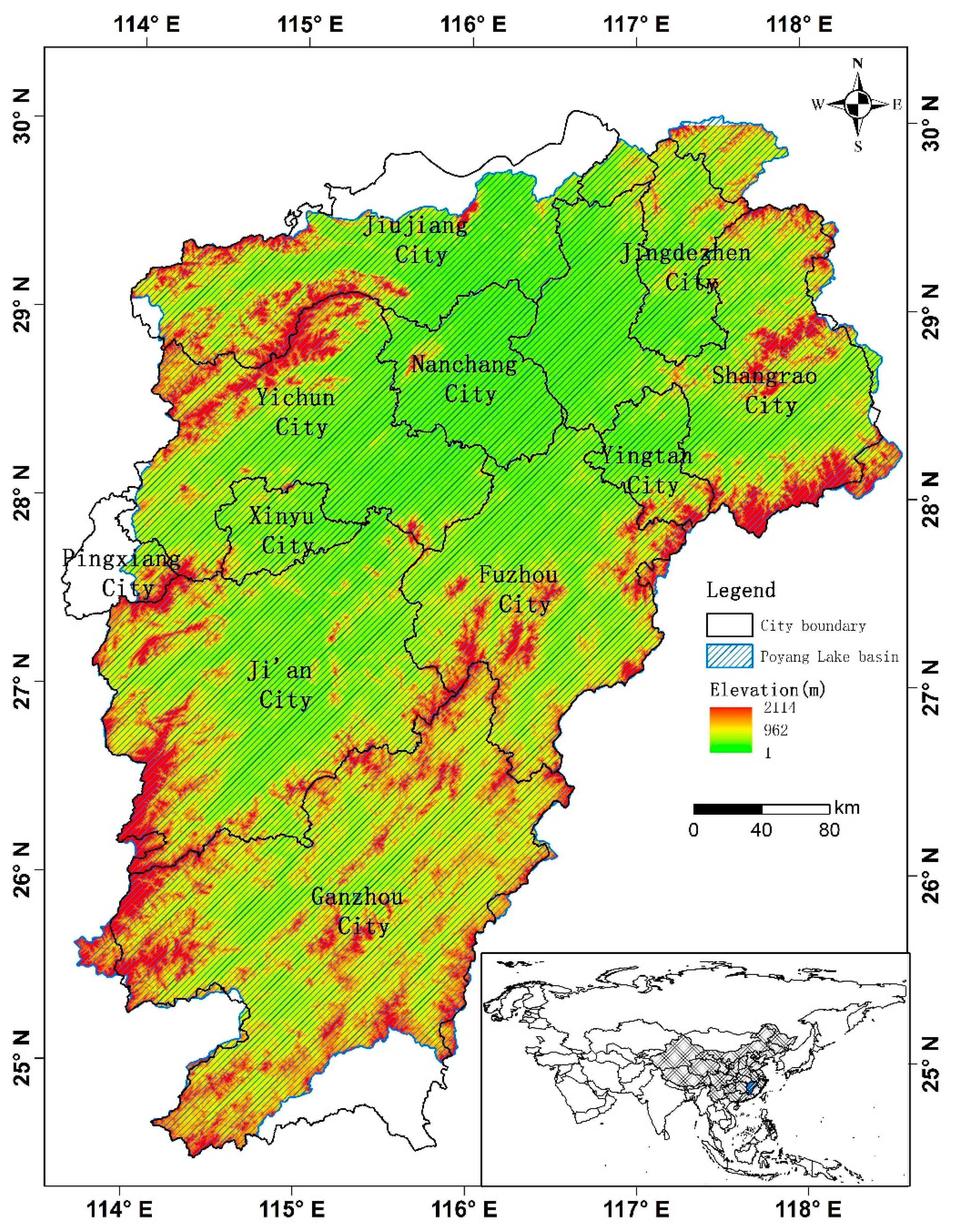
3. Case Study and Data

Poyang Lake (as illustrated in Figure 2), as a precious gourd, lies in the Yangtze River system, is a paradise for migratory birds, is the largest freshwater lake in China, and was included in a list of international important wetlands by the United Nations Educational, Scientific, and Cultural Organization (UNESCO) in 1995. Poyang Lake basin is mainly constituted by five rivers (the Ganjiang, Fuhe, Xinjiang, Raohe, and Xiushui) and their tributaries, and discharges to the Yangtze River through a narrow outlet in the north, forming a convergent drainage system with the convergence center in Poyang Lake. The fertile wide alluvial plains located downstream of the Ganjiang and Fuhe catchments are vital rice growing regions in China, with an irrigation area over 10,000 ha. The Poyang Lake basin is located at a longitude of 113°34′ to 118°28′ and a latitude of 24°29′ to 30°04′, covering an area of 162,225 km², with most catchment areas in Jiangxi Province (156,743 km², 96.6%). Therefore, this thesis utilized water consumption and GDP data from Jiangxi Province to study the relationship between water consumption and economic development in the Poyang Lake basin. Although Poyang Lake basin is under relatively abundant water resource condition, regional water resource-related problems, including the asynchrony of inflow and water demand, unreasonable water use structures, low water utilization efficiency, and resource-based water deficits caused by less seasonal inflows in the Ganjiang tributaries (such as the Yuanshui, Jinjiang, etc.), have been exacerbated due to the rapid regional socioeconomic development [42]. Analyzing the relationship between water use and economic growth in Poyang Lake basin will be useful for proposing response strategies and managing water resources.

As mentioned before, Jiangxi Province covers almost 96% of the area of the Poyang Lake basin, and the data about water consumption and economic development were obtained from the Jixangxi Province Water Resource Bulletins, Jiangxi Province Statistical Yearbook. The case period of 2003–2016 was selected because of two reasons. First, rapid economic growth occurred in China during this period. Second, an obvious changing water consumption trajectory appeared with the implementation of water-saving policies in 2003. GDP data were adjusted at a constant 2003 price to eliminate the effects of inflation. The results in this paper were obtained by using MATLAB2014a, ArcGis 10.0, and StataSE15.

4. Results

In this section, we present the results in terms of three aspects. First, the variation in trend items of water consumption and GDP time series data obtained by using the Hodrick–Prescott filtering method in the Poyang Lake basin are presented. Second, the decoupling status between water consumption and the GDP of each city in the Poyang Lake basin are exhibited based on original and trend time series data. Third, the spatial aggregation characteristics and spatial gravity center migration status of the related parameters (e.g., trend components of water consumption and GDP time series data, decoupling status measured by the decoupling index) in the Poyang Lake basin are displayed.

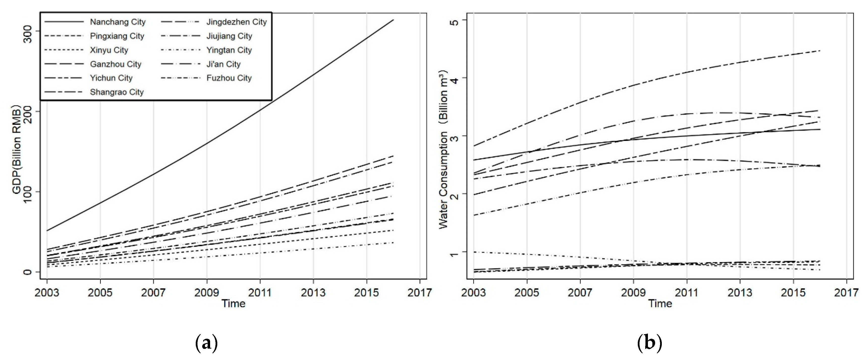
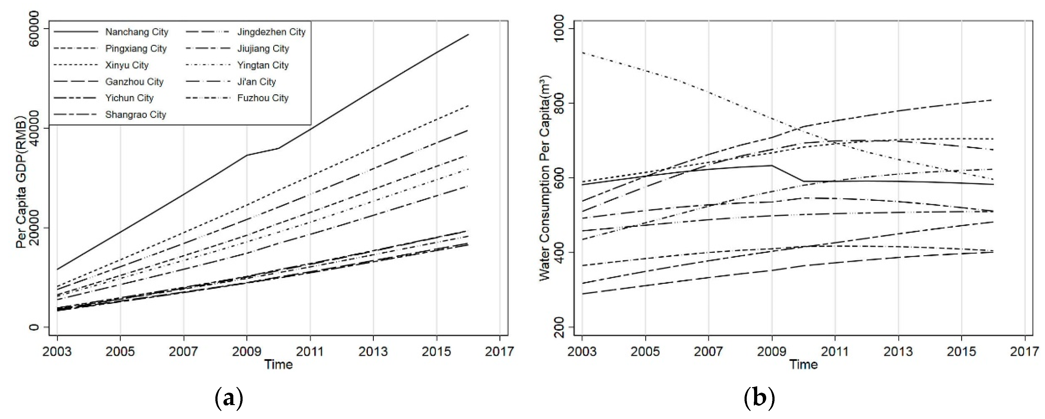
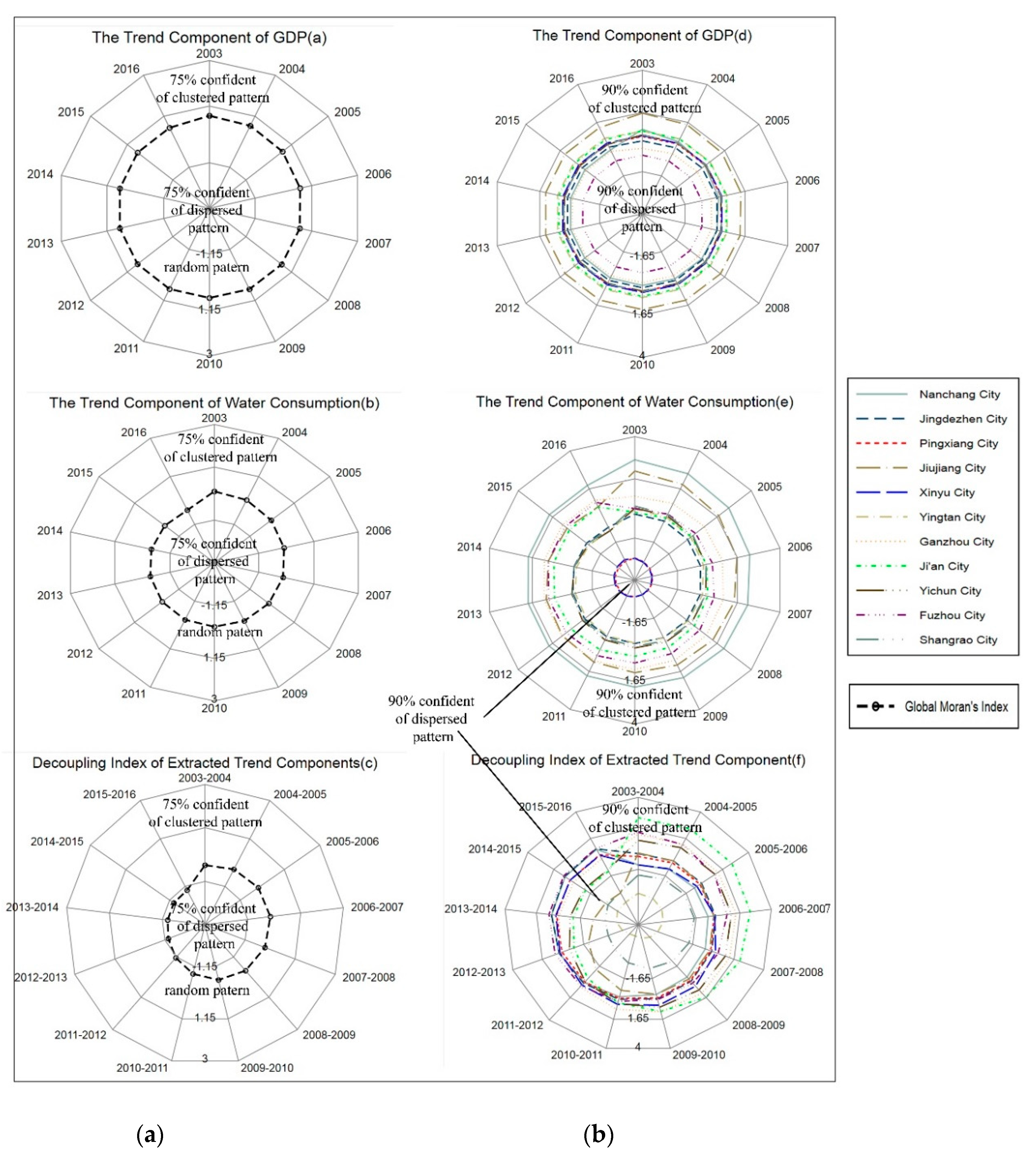
4.1. The Variation in Trend Components of Water Consumption and GDP Time Series Data in Poyang Lake Basin

Figure 3 and Figure 4 show the variation in trend items of water consumption and GDP time series data in each city of the Poyang Lake basin and in Jiangxi Province by using the Hodrick–Prescott filtering method introduced in Section 2.1. As illustrated in Figure 3a, the extracted trend term of GDP showed an increasing trend. During the period of 2003 to 2016, Nanchang City had the fastest economic growth rate: the GDP increased by 508.8%, changing from 51.6 billion to 314 billion RMB (Ren Min Bi, China Yuan). However, Yingtan City had the slowest economic growth rate: the GDP only increased by 456.1%, changing from 6.6 billion to 36.7 billion RMB.

As illustrated in Figure 3b, the trend items of water consumption in each city had their own variation trends:

• During the period from 2003 to 2016, Yichun City, Ganzhou City, and Shangrao City presented an increasing trend, with growth rates of 58%, 47%, and 63%, respectively;
• Ji’an City displayed an increasing trend at first, and then slightly declined. Water consumption increased from 2.36 billion m³ in 2003 to 3.39 billion m³ in 2012. During the period from 2012 to 2016, water consumption in Ji’an City decreased to 3.32 billion m³. There existed a similar trend pattern between Jiujiang City and Ji’an City. In Jiujiang City, water consumption increased from 2.26 billion m³ in 2003 to 2.58 billion m³ in 2012. During the period from 2012 to 2016, water consumption decreased to 2.47 billion m³ in Jiujiang City;
• Nanchang City and Fuzhou City displayed an increasing trend at first, and then became nearly steady. Water consumption in Nanchang City increased from 2.58 billion m³ in 2003 to 3 billion m³ in 2009 and was basically maintained at 3 billion m³ after 2009. Water consumption in Fuzhou City increased from 1.63 billion m³ in 2003 to 2.4 billion m³ in 2013 and then was basically maintained at 2.4 billion m³ after 2013;
• Jingdezhen City, Xinyu City, and Pingxiang City had less variation in water consumption than others, seeming to level off at around 7.5 billion m³, 7.3 billion m³, and 7.2 billion m³, respectively;
• Yintan City displayed a decreasing trend, with a decrease rate of 31%.

As can be seen from Figure 4, the economic trend of Jixangxi Province presented an increasing trend. By the end of 2016, the GDP of Jixangxi Province still kept increasing, while water consumption gradually slowed down after 2009 and approached a steady status at the end of 2016.

Figure 5a shows the average trends of extracted trends of GDP and water consumption by weighting the number of inhabitants and users of water, respectively. In Figure 5a, Nanchang City owned the maximum per capita GDP, while Shangrao City had the minimum per capita GDP. The per capita GDP of the all cities in Poyang Lake basin showed an increasing trend over the period 2003-2017. As illustrated in Figure 5b, the per capita water consumption of Yingtan City had the fastest decreasing rate, changing from 935.5 m³ in 2003 to 596.5 m³ in 2016. The per capita water consumption of Yichun City, Fuzhou City, Shangrao City, and Ganzhou City displayed an increasing trend. The per capita water consumption of Ji’an City, Nanchang City, Jiujiang City, and Pingxiang City showed an increasing trend at first and then slightly declined. Xinyu City displayed an increasing trend between the period of 2003 and 2011 and maitained basically at the value of 700 m³ after 2011.

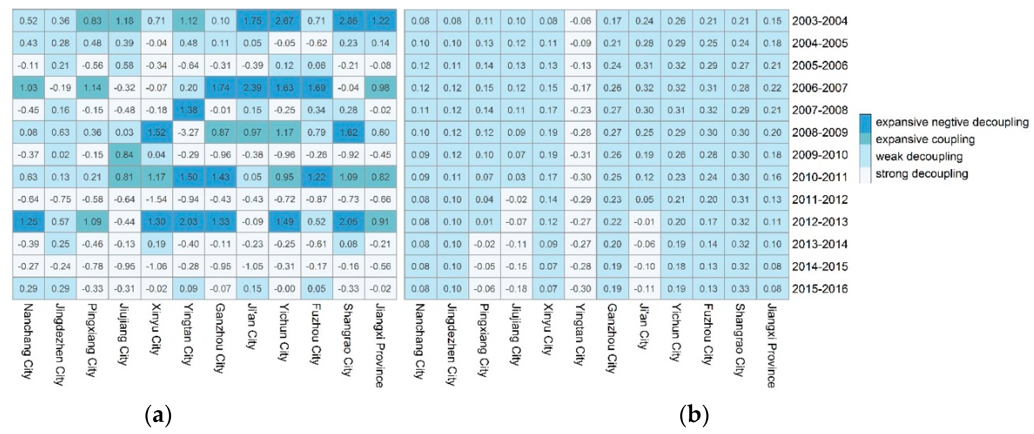
4.2. Results of Decoupling Analysis in Poyang Lake Basin

This thesis calculated the decoupling elasticity index between water consumption and the GDP of each city in Jiangxi Province of Poyang Lake basin by using the method introduced in Section 2.2. As illustrated in Figure 6a, the decoupling relationship between water consumption and GDP by using original time series data could be characterized by four categories: expansive negative decoupling (END), expansive coupling (EC), weak decoupling (WD), and strong decoupling (SD). The results of the decoupling analysis displayed volatility, and the variation in decoupling status was discontinuous. The status of water consumption decoupled from economic growth in overall cities occurred after 2013, but during the period from 2003 to 2013, the decoupling statuses were fluctuant in each city. For example, Nanchang City exhibited a fluctuant status between weak decoupling and strong decoupling during the periods 2004–2006, 2008–2010, and 2010–2012; Pingxiang City exhibited a fluctuant status between coupling and decoupling during the periods 2003–2006, 2006–2012, and 2012–2016; and Fuzhou City exhibited a fluctuant status between decoupling and negative decoupling during the periods 2003–2007 and 2007–2011. As illustrated in Figure 6b, the results of the decoupling analysis presented more stably by means of extracting the trend components from water consumption and GDP time series data, which could eliminate the influence of periodic factors. There were three categories of decoupling statuses: the status of always staying in weak decoupling, the status of transferring from weak decoupling to strong decoupling, and the status of always staying in strong decoupling. Nanchang City, Jingdezhen City, Xinyu City, Ganzhou city, Yichun City, Fuzhou City, and Shangrao City belonged to the first category. Pingxiang City, Jiujiang City, and Ji’an City experienced a transformation from a weak decoupling status to a strong decoupling status at year 2013, 2011, and 2012, respectively. Yingtan City always stayed in a strong decoupling status. As for Jiangxi Province, there existed a fluctuant status between decoupling and coupling using original water consumption and GDP time series data during the periods 2004–2007, 2007–2011, and 2011-2012, respectively (Figure 6a), while the decoupling status was more stable by extracting the trend components (Figure 6b).

The numbers in the boxes represent the numerical values of the decoupling elasticity index. The smaller the numerical value is, the better the decoupling status was and vice versa. As for the regions in a weak decoupling status, a transformation in the numerical value of the decoupling elasticity index from 0.08 to 0.12 and from 0.12 to 0.08 showed that Nanchang City experienced a decoupling status variation, although it always stayed in a weak decoupling status. Jingdezhen City, Xinyu City, Ganzhou City, Yichun City, Fuzhou City, and Jiangxi Province had the same kind of decoupling elasticity index transformation, while Shangrao City exhibited an increasing trend in the decoupling elasticity index. Thus, except for Shangrao City, the other regions will surely step into a strong decoupling status in the future. On the whole, water consumption basically decoupled from GDP growth in Poyang Lake basin.

4.3. Spatial Variation Characteristics of Decoupling Statuses in Poyang Lake Basin

In Section 4.1 and Section 4.2, we mainly focused on the variation in the relationship between water consumption and GDP on a temporal scale. However, their spatial characteristics also played an important role in interpreting the water–economy relationship and generating water resource management strategies. The Global Moran’s Index and Anselin Local Moran’s Index were calculated by using the equation introduced in Section 2.3 based on extracted components of water consumption and GDP time series data expressed as attribute values. As illustrated in Figure 7a, the Global Moran’s Index Score $Z_I$ of GDP and water consumption in Poyang Lake basin basically changed between −1.15 and 1.15 during the period 2003–2008 and belonged to a random pattern in Jiangxi Province. Namely, there existed no spatial autocorrelation in both GDP and water consumption, and the spatial aggregation characteristics of GDP and water consumption had not occurred yet in Poyang Lake basin. However, for the decoupling index in Poyang Lake basin, the Global Moran’s Index Score $Z_I$ exhibited a quite different phenomenon, with a decreased trend from 2003 to 2011 approximating a 75% confidence interval in dissimilar clusters from 2011 to 2012 and staying at a 75% confidence interval in dissimilar clusters from 2012 to 2016, which indicated that the spatial aggregation characteristics of the decoupling index appeared. Namely, the characteristics of a slower growth rate of water consumption than of GDP occurred, which reflected regional differences in the economic benefits brought by water utilization. Figure 7b illustrates the variation in the Anselin Local Moran’s Index Score. As for the extracted trend item of GDP, whole cities showed a pattern of randomness. As for the extracted trend item of water consumption, a pattern of high–high similar clusters occurred in Jiujiang City and Nanchang City, with quite different appearances between them. Jiujiang City exhibited a pattern of high–high similar clusters from 2003 to 2006, which transformed into a random pattern in the next few years, while Nanchang City always stayed in a pattern of high–high similar clusters, which meant that both Nanchang City and neighboring cities (including Yichun City and Jiujiang City) experienced a relatively high level of water consumption. Pingxiang City and Xinyu City always stayed in a pattern of low–high dissimilar clusters. The other cities displayed a pattern of randomness. As for the decoupling index, Nanchang City, Jingdezhen City, Pingxiang City, Xinyu City, Ganzhou City, Yichun City, and Fuzhou City stayed in a random pattern. Yingtan City and Shangrao City showed patterns of low–high and high–low dissimilar clusters at a 90% confidence interval, respectively. The decoupling index indicated the ratio of the growth rate of water consumption to GDP. As for the status of decoupling, the smaller the decoupling index was, the better the degree of decoupling water consumption from economic growth was. Jiujiang City exhibited a random pattern from 2003 to 2012, which transformed into a pattern of low–high dissimilar clusters with a 90% confidence interval in 2012. Ji’an City exhibited a pattern of high–high similar clusters from 2003 to 2008, which transformed into a random pattern after 2008.

Figure 8 shows the spatial migration characteristics of GDP, water consumption, and the decoupling index in Poyang Lake basin. The geodetic coordinates of the municipal administrative center in Jiangxi Province were calculated based on the 54 Beijing Coordinate in Arcgis 10.0. As illustrated in Figure 6, the GDP gravity center gradually approximated Nanchang City, the capital of Jiangxi Province, during the period 2003–2016, with a migration direction of northeast and a migration distance of about 3.3 km. However, the migration directions of the water consumption gravity center and the decoupling index gravity center were different from GDP. The migration direction of the water consumption gravity center was southwest during 2003–2012, with a migration distance of about 8.1 km and after 2012, the direction shifted to southeast, with a migration distance of about 2.4 km. The migration direction of the decoupling index gravity center was similar to that of water consumption, which also showed characteristics of shifting from southwest to southeast. The migration distance was about 13.9 km during 2003–2009 and about 103.4 km during 2009–2016.

5. Discussion

5.1. Interpretation of the Several Decoupling Statuses

As can be seen from Figure 1, statuses of strong negative decoupling, weak negative decoupling, recessive coupling, and recessive decoupling exist in a period of economic recession, while statuses of expansive negative decoupling, expansive coupling, weak decoupling, and strong decoupling appear in a period of economic development. Based on the meaning of each decoupling status (see Table 1), the best water–economy status is strong decoupling, which indicates a decrease in water consumption as well as an increase in economic output value, while the worst status is strong negative decoupling, which indicates an increase in water consumption as well as a decrease in economic output value. There only appeared four types of statuses (expansive negative decoupling, expansive coupling, weak coupling, and strong decoupling) in Poyang Lake basin because it stayed in a period of economic development. The expansive negative decoupling status indicates that water consumption keeps increasing while the economy keeps increasing and the variation rate of water consumption is faster than that of the economy, which is an unsustainable pattern with low water resource use efficiency. The expansive coupling status indicates that the variation rate of water consumption is nearly the same as that of the economy, which reflects a medium water resource use efficiency. The weak decoupling status, which means the variation rate of water consumption is slower than that of the economy, represents a region having a relatively high water resource use efficiency. From these statuses, it can be inferred that coupling is a transition status between negative decoupling and decoupling. Expansive decoupling evolves into expansive negative decoupling when the growth rate of water consumption is faster than that of the economy: Otherwise, expansive coupling evolves into weak decoupling. Recessive coupling evolves into recessive decoupling when the reduction rate of water consumption is faster than that of the economy: Otherwise, expansive coupling evolves into weak negative decoupling. Strong negative decoupling and strong decoupling are two completely opposite statuses representing the most disadvantageous and advantageous status between water consumption and economic development, respectively.

Poyang Lake basin basically stayed in a weak decoupling and strong decoupling status, and the weak decoupling status had a tendency toward the strong decoupling status (Section 4.2). The reason for the water consumption decrease probably was the use of more efficient equipment with economic development and an industrial structure adjustment that resulted in a detriment to agriculture. Thus, the water use pattern in the Poyang Lake basin is sustainable to a certain extent.

5.2. Explanation of Global Moran’s Index and Anselin Local Moran’s Index

The scores of Global Moran’s Index $Z_I$ and Anselin Local Moran’s Index $Z_I$ were used to determine whether to reject the null hypothesis of the complete spatial randomness of the values associated with the features (e.g., GDP, water consumption, decoupling index) or not. In a Global Moran’s Index analysis, a positive score for a feature indicates apparent similarity, with a spatial clustering of either high or low values, while a negative score for a feature indicates apparent dissimilarity, with a spatial outlier at a given statistical significance (e.g., the 0.25 level, 0.1 level, 0.01 level). In an Anselin Local Moran’s Index analysis, a positive score indicates if the feature has a high value and is surrounded by features with high values (high–high) or if the feature has a low value and is surrounded by features with low values (low–low). A negative score indicates if the feature has a high value and is surrounded by features with low values (high–low) or if the feature has a low value and is surrounded by features with high values (low–high). There exists some relationship between the magnitude of the decoupling index value and the spatial characteristics it presents. The lower the value for the decoupling index was, the better the decoupling status of the city was when the regions belonged to decoupling. As for Yingtan City, the spatial aggregation characteristics of low–high meant that the decoupling index of Yingtan City was smaller than that of its surrounding cities: Nanchang City, Shangrao City, and Fuzhou City. Therefore, the decoupling status of Yingtan City should have been better than its surrounding cities, which could be proven from the results in Figure 3b because strong decoupling is better than weak decoupling.

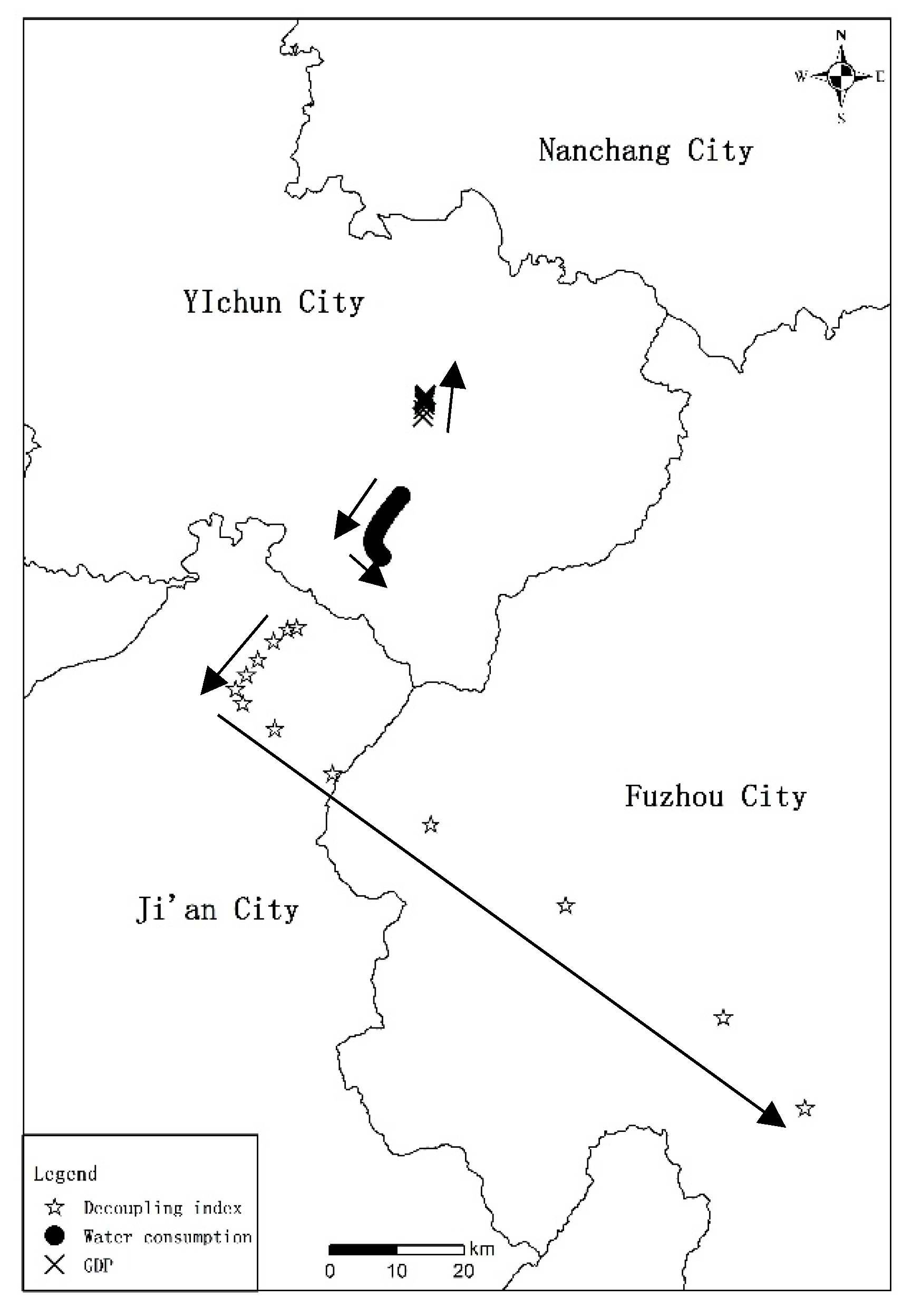
5.3. The Migration Significance of the Spatial Gravity Center for GDP, Water Consumption, and the Decoupling Index

The gravity center could be regarded as the point where the maximum value of the regional feature lay, according to the definition. Therefore, the GDP gravity center was the point where the maximum economic output value occurred, as well as the same meaning of water consumption gravity center and the decoupling index center. A high decoupling index reflected that the water consumption rate was faster than GDP growth. To some extent, a high decoupling index presented a pattern of relatively low water utilization efficiency. Therefore, the migration of the decoupling index gravity center exhibited a variation in low water utilization efficiency. As illustrated in Figure 5, the migration direction of the GDP gravity center was opposite to the migration direction of the water consumption gravity center, which meant it was not necessary to consume much more water to promote economic growth for the region with the largest economic output value. This is basically in consistent with the result that the Poyang Lake basin is in a decoupling status at present. As illustrated in Figure 5, the migration direction of the water consumption gravity center was similar to the migration direction of the decoupling index gravity center, which meant that the region of low water resource utilization efficiency and the region of the largest economic output value were at different locations. Therefore, it can be inferred that the water resource utilization efficiency was relatively high and the water use pattern was sustainable to a certain extent.

6. Conclusions

This study explored the coordinated development of water resource utilization and economic growth both at a temporal and spatial scale in the Poyang Lake basin. The research data used mainly came from Jiangxi Province because its area accounts for more than 96% of the Poyang Lake basin. The temporal decoupling statuses between water use and economic growth were obtained based on original and trend extracted data through the Tapio decoupling model. The spatial analysis of water consumption, economic growth, and decoupling statuses was tackled through the Global Moran’s Index, Local Moran’s Index, and spatial gravity theory. The analysis led to the following conclusions:

• Decoupling statuses (based on original and extracted data) between water consumption and economic growth showed a significant difference. The original sequence were volatile, while the trend extracted sequence were steady with the elimination of cyclic factors;
• In the Poyang Lake basin, water consumption basically decoupled from economic growth, and the decoupling status characteristics could be divided into three categories. The first kind always kept a weak decoupling status, including Nanchang City, Jingdezhen City, Ganzhou City, Fuzhou City, and Shangrao City. The second kind experienced a status transformation from weak decoupling to strong decoupling, including Pingxiang City, Jiujiang City, and Ji’an City. The third kind always kept a strong decoupling status (only Yingtan City);
• In the Poyang Lake basin, from a global perspective, GDP and water consumption exhibited randomness characteristics, while the decoupling index exhibited spatial outlier characteristics. From a local perspective, GDP exhibited a random pattern, the water consumption of some areas (e.g., Nanchang City) exhibited a spatial clustering of high–high characteristics, and the decoupling index of some areas (e.g., Yingtan City, Shangrao City, Jiujiang City) exhibited a spatial outlier of low–high or high–low characteristics;
• With respect to the migration of the spatial gravity center, the direction of GDP was opposite to water consumption, while the direction of the decoupling index was similar to water consumption, which meant it was not necessary to consume much more water to promote economic growth for the region with the largest economic output value. Therefore, the water use pattern in the Poyang Lake basin was sustainable to a certain extent.

References

1. Rosegrant, M.W.; Ringler, C.; Zhu, T. Water for Agriculture: Maintaining Food Security under Growing Scarcity. Annu. Rev. Environ. Res. 2010, 24, 205–222. [Google Scholar] [CrossRef]
2. Nazemi, A.; Madani, K. Urban Water Security: Emerging Discussion and Remaining Challenges. Sustain. Cities Soc. 2018, 41, 925–928. [Google Scholar] [CrossRef]
3. Vörösmarty, C.J.; Green, P.; Salisbury, J.; Lammers, R.B. Global Water Resources: Vulnerability from Climate Change and Population Growth. Science 2000, 289, 284–288. [Google Scholar] [CrossRef]
4. Sun, S.; Fang, C. Water Use Trend Analysis: A Non-Parametric Method for the Environmental Kuznets Curve Detection. J. Clean. Prod. 2018, 172, 497–507. [Google Scholar] [CrossRef]
5. Li, Y.; Lu, L.; Tan, Y.; Wang, L.; Shen, M. Decoupling Water Consumption and Environmental Impact on Textile Industry by Using Water Footprint Method: A Case Study in China. Water 2017, 9, 124. [Google Scholar] [CrossRef]
6. OECD. Indicators to Measure Decoupling of Environmental Pressure from Economic Growth. 2002. Available online: http://www.oecd.org/environment/indicators-modelling-outlooks/1933638.pdf (accessed on 16 May 2019).
7. Vehmas, J.; Kaivo-oja, J.; Luukkanen, J. Global Trends of Linking Environmental Stress and Economic Growth; Finland Futures Research Centre: Turku, Finnlands, 2003; pp. 6–9. [Google Scholar]
8. Vehmas, J.; Luukkanen, J.; Kaivo-oja, J. Linking Analyses and Environmental Kuznets Curves for Aggregated Material Flows in the EU. J. Clean. Prod. 2007, 15, 1662–1673. [Google Scholar] [CrossRef]
9. Tapio, P. Towards a Theory of Decoupling: Degrees of Decoupling in the EU and the Case of Road Traffic in Finland between 1970 and 2001. Transp. Policy 2005, 12, 137–151. [Google Scholar] [CrossRef]
10. Yu, Y.; Zhou, L.; Zhou, W.; Ren, H.; Kharrazi, A.; Ma, T.; Zhu, B. Decoupling Environmental Pressure from Economic Growth on City Level: The Case Study of Chongqing in China. Ecol. Indic. 2017, 75, 27–35. [Google Scholar] [CrossRef]
11. Wang, Q.; Li, R.; Jiang, R. Decoupling and Decomposition Analysis of Carbon Emissions from Industry: A Case Study from China. Sustainability 2016, 8, 1059. [Google Scholar] [CrossRef]
12. Wang, Z.; Zhao, L.; Mao, G.; Wu, B. Eco-Efficiency Trends and Decoupling Analysis of Environmental Pressures in Tianjin, China. Sustainability 2015, 7, 15407–15422. [Google Scholar] [CrossRef]
13. Yu, Y.; Chen, D.; Zhu, B.; Hu, S. Eco-Efficiency Trends in China, 1978–2010: Decoupling Environmental Pressure from Economic Growth. Ecol. Indic. 2013, 24, 177–184. [Google Scholar] [CrossRef]
14. Song, Y.; Zhang, M. Using a New Decoupling Indicator (ZM Decoupling Indicator) to Study the Relationship between the Economic Growth and Energy Consumption in China. Nat. Hazards 2017, 88, 1013–1022. [Google Scholar] [CrossRef]
15. Wang, H.; Hashimoto, S.; Yue, Q.; Moriguchi, Y.; Lu, Z. Decoupling Analysis of Four Selected Countries. J. Ind. Ecol. 2013, 17, 618–629. [Google Scholar] [CrossRef]
16. Acheampong, E.N.; Swilling, M.; Urama, K. Developing a Framework for Supporting the Implementation of Integrated Water Resource Management (IWRM) with a Decoupling Strategy. Water Policy 2016, 18, 1317–1333. [Google Scholar] [CrossRef]
17. Zhong, T.Y.; Huang, X.J.; Han, L.; Wang, B.Y. Review on the Research of Decoupling Analysis in the Field of Environments and Resource. J. Nat. Res. 2010, 25, 1400–1412. (In Chinese) [Google Scholar]
18. Li, N.; Zhang, J.Q.; Wang, L. Decoupling and Water Footprint Analysis of the Coordinated Development between Water Utilization and the Economy in Urban Agglomeration in the Middle Reaches of the Yangtze River. China Popul. Res. Environ. 2017, 27, 202–208. (In Chinese) [Google Scholar]
19. Urama, K.C.; Bjornse, P.K.; Reiegels, N.; Vairavamoorthy, K.; Herrick, J.; Kauppi, L.; Mcneely, J.A.; Mcglade, J.; Eboh, E.; Smith, M. United Nations Environment Programme (UNEP) IRP Report-Options for Decoupling Economic Growth from Water Use and Water Pollution; Technical Report; United Nations Environment Programme: Paris, France, 2016. [Google Scholar]
20. Wang, Q.; Jiang, R.; Li, R. Decoupling Analysis of Economic Growth from Water Use in City: A Case Study of Beijing, Shanghai, and Guangzhou of China. Sustain. Cities Soc. 2018, 41, 86–94. [Google Scholar] [CrossRef]
21. Wang, S.; Li, R. Toward the Coordinated Sustainable Development of Urban Water Resource Use and Economic Growth: An Empirical Analysis of Tianjin City, China. Sustainability 2018, 10, 1323. [Google Scholar] [CrossRef]
22. Zhang, Z.L.; Xue, B.; Pang, J.; Chen, X. The Decoupling of Resource Consumption and Environmental Impact from Economic Growth in China: Spatial Pattern and Temporal Trend. Sustainability 2016, 8, 222. [Google Scholar] [CrossRef]
23. Wang, B.Q. Study on the Relationship between Chinese Economic Growth and Water Resources Based on the Decoupling Analysis. Master’s Thesis, Degree-Lanzhou University, Lanzhou, China, 1 June 2015. (In Chinese). [Google Scholar]
24. Yu, Z.; Yang, Q.S. Decoupling Agricultural Water Consumption and Environmental Impact from Crop Production Based on the Water Footprint Method: A Case Study for the Heilongjiang Land Reclamation Area, China. Ecol. Indic. 2014, 43, 29–35. [Google Scholar] [CrossRef]
25. Zhu, H.; Li, W.; Yu, J.; Sun, W.; Yao, X. An Analysis of Decoupling Relationships of Water Uses and Economic Development in the Two Provinces of Yunnan and Guizhou During the First Ten Years of Implementing the Great Western Development Strategy. Procedia Environ. Sci. 2013, 18, 864–870. [Google Scholar] [CrossRef]
26. Rock, M.T. Freshwater Use, Freshwater Scarcity, and Socioeconomic Development. J. Environ. Dev. 1998, 7, 278–301. [Google Scholar] [CrossRef]
27. Duarte, R.; Pinilla, V.; Serrano, A. Is There an Environmental Kuznets Curve for Water Use? A Panel Smooth Transition Regression Approach. Econ. Model. 2013, 31, 518–527. [Google Scholar] [CrossRef]
28. Cole, M.A. Economic Growth and Water Use. Appl. Econ. Lett. 2004, 11, 1–4. [Google Scholar] [CrossRef]
29. Ma, J.; Yan, B.S. Based on the Envrionmental Kuznets Theory of Relationship between Economic Development and Water Use Efficiency of Morphological Research-From the Data of 11 Provinces during the Period of 2002-013. J. Audit Econ. 2016, 4, 21–128. (In Chinese) [Google Scholar]
30. Zhao, X.; Fan, X.; Liang, J. Kuznets Type Relationship between Water Use and Economic Growth in China. J. Clean. Prod. 2017, 168, 1091–1100. [Google Scholar] [CrossRef]
31. Katz, D. Water Use and Economic Growth: Reconsidering the Environmental Kuznets Curve Relationship. J. Clean. Prod. 2015, 88, 205–213. [Google Scholar] [CrossRef]
32. Ke, W.; Sha, J.; Yan, J.; Zhang, G.; Wu, R. A Multi-Objective Input–Output Linear Model for Water Supply, Economic Growth and Environmental Planning in Resource-Based Cities. Sustainability 2016, 8, 160. [Google Scholar] [CrossRef]
33. Bao, C.; Chen, X. The Driving Effects of Urbanization on Economic Growth and Water Use Change in China: A Provincial-Level Analysis in 1997–2011. J. Geogr. Sci. 2015, 25, 530–544. [Google Scholar] [CrossRef]
34. Bao, C.; He, D. The Causal Relationship between Urbanization, Economic Growth and Water Use Change in Provincial China. Sustainability 2015, 7, 16076–16085. [Google Scholar] [CrossRef]
35. Hodrick, R.J.; Prescott, E.C. Postwar US Business Cycles: An Empirical Investigation. J. Money Credit Bank. 1997, 29, 1–16. [Google Scholar] [CrossRef]
36. Wang, W.S.; Jin, J.L.; Ding, J. Stochastic Hydrology, 2nd ed.; China Water and Power Press: Beijing, China, 2008. (In Chinese) [Google Scholar]
37. Tobler, W.R. Computer Movie Simulating Urban Growth in Detroit Region. Econ. Geogr. 1970, 46, 234–240. [Google Scholar] [CrossRef]
38. Moran, P. Notes on Continuous Stochastic Phenomena. Biometrika 1950, 37, 17–23. [Google Scholar] [CrossRef] [PubMed]
39. Anselin, L. Local Indicators of Spatial Association-LISA. Geogr. Anal. 1995, 27, 93–115. [Google Scholar] [CrossRef]
40. ArcGIS Resources. Available online: http://resources.arcgis.com/zh-cn/help/main/10.1/index.html#/na/005p00000006000000/ (accessed on 14 February 2019).
41. Xv, J.H.; Yue, W.Z. Evolvement and Comparative Analysis of the Population Center Gravity and the Economy Gravity Center in Recent Twenty Years in China. Sci. Geogr. Sin. 2001, 21, 385–389. [Google Scholar]
42. Yang, Y.S.; Xv, X.F.; Li, R.F. Research on Water Distribution and Water Right System Construction in Poyang Lake Basin, 1st ed.; China Water and Power Press: Beijing, China, 2011. (In Chinese) [Google Scholar]
Figure 1. Judgments of coupling and decoupling statuses (quoted from Tapio et al., 2005 [9]).
Water 11 01027 g001
Figure 2. Geographic location of the Poyang Lake basin.
Water 11 01027 g002
Figure 3. The variation in the extracted trend components of Gross Domestic Product (GDP) (a) and water consumption (b) time series data in each city of Jiangxi Province, Poyang Lake basin.
Water 11 01027 g003
Figure 4. The variation in the extracted trends of GDP (a) and water consumption (b) time series data in Poyang Lake basin.
Water 11 01027 g004
Figure 5. The variation in the extracted trends of per capita GDP (a) and per capita water consumption (b) in Poyang Lake basin.
Water 11 01027 g005
Figure 6. The decoupling results obtained from raw water consumption and GDP time series data (a) and from extracted trend components of water consumption and GDP time series data (b) in each city of Jiangxi Province in the Poyang Lake basin. The numbers in the boxes represent the decoupling elasticity index. The smaller the numerical value is, the better the decoupling status was and vice versa.
Water 11 01027 g006
Figure 7. The variation of in the Global Moran’s Index Score ZI (a) and the Local Moran’s Index Score ZIi (b) during 2003–2016 in each city of Jiangxi Province, Poyang Lake basin.
Water 11 01027 g007
Figure 8. The spatial gravity center migration of the decoupling index, water consumption, and GDP during 2003–2016 in Poyang Lake basin.
Water 11 01027 g008