Simulation of the Surface Energy Flux and Thermal Stratification of Lake Taihu with Three 1-D Models


1
Yale-Nanjing University of Information Science and Technology Center on Atmospheric Environment, Nanjing 210044, China
2
School of Atmospheric Physics, Nanjing University of Information Science and Technology, Nanjing 210044, China
*
Author to whom correspondence should be addressed.
Water 2019, 11(5), 1026; https://doi.org/10.3390/w11051026
Submission received: 4 March 2019
/
Revised: 30 April 2019
/
Accepted: 14 May 2019
/
Published: 16 May 2019
(This article belongs to the Special Issue Water Quality Monitoring and Modeling Research)
Abstract
:The accurate simulation of lake-air exchanges can improve weather and climate predictions, quantify the lake water cycle and provide evidence for water demand management and decision making. This paper analyzes the thermal stratification and surface flux of eastern Lake Taihu and evaluates three common surface models: CLM4-LISSS, E-ε and LAKE. The results show that the thermal stratification and lake-air exchanges are greatly affected by the weather conditions and have obvious diurnal variations in the Lake Taihu. The eddy exchange coefficient (EEC) in the thermodynamic equation varies greatly with the weather conditions and the water depth too, and an accurate parameterization scheme is important for the temperature simulations. The lake surface temperature simulation results of the CLM4-LISSS model have the highest accuracy due to the more accurate EEC simulation, with a correlation coefficient (CC) of 0.94 and a root mean square error (RMSE) of 0.85 °C, and latent flux simulation with a CC of 0.78 and a RMSE of 55.32 W m−2. Moreover, the submerged plants in shallow water have obvious influences on the radiation, thermal transferring and eddy motion. The E–ε model can accurately simulate the surface temperature with submerged plants consideration, though a better scheme to deal with surface flux and turbulence dissipation in the areas of submerged plants is still need to be developed. The physical process in the LAKE model is comprehensive, while when it is used to simulate Lake Taihu and other shallow lakes, the EEC is large and needs to be adjusted.
1. Introduction
Surface modeling of lakes is a critical process to estimate the fluxes on the lake surface for numerical simulations of weather and climate [1]. The accuracy of the results is important for weather prediction [2,3,4], climate change [5,6] and pollutant dispersion simulations [7,8]. Hydromechanics and thermodynamics provide theoretical framework for the development of mathematical models for lakes and reservoirs. At present, the 1-D models, which are widely used in the field of atmospheric science, assume that the physical properties of lake water are horizontally uniform and only the heat transfer of lake water in the vertical direction is considered. Three schemes have been proposed for lake surface process estimates: (1) two-layer parametric models based on similarity theory, such as Flake [9]; (2) 1-D thermal diffusion models with parameterized eddy diffusion in water, including the Hostertler model [10], the MINLAKE scheme [11], LISSS [12,13]; and (3) more sophisticated 1-D turbulence closure schemes that consider the turbulent motion of water, such as the Lagrange DYRESM model [14], the E–ε SIMSTRAT turbulent closure model [15] and the LAKE model [16,17].
Comparisons and assessments of different lake models are commonly performed. The LAKEMIP project aims to confirm the essential physical processes that can be represented by models of lake physics, lake chemistry, lake hydrology and lake biology (especially climate simulations and weather forecasting) in different applications and further explore and improve their parameterization schemes [18]. Stepanenko et al. used five lake models (FLake, CLM4-LISSS, LAKE, LAKEoneD and Simstrat) to simulate and evaluate Sparking Lake, Lake Kivu, Kossenbkatter and Valkea-Kotinen. All of the models can simulate the lake surface temperature well but not the water temperature. This phenomenon occurs because the calculation of the surface temperature is based on the Monin-Obukhov similarity theory, whereas the calculation of the water temperature is influenced by the different eddy exchange coefficients (EECs) used in different lake models. Sensitivity tests of lake depth indicate that accurate lake depths can improve the simulation results.
In lake models, the parameter settings, including the lake depth, internal EEC, extinction coefficient, surface roughness length and salinity, are important for lake thermodynamic simulations and must be adjusted according to the lake characteristics [19]. In the lake simulation with different depths, the key parameters in the model, such as the EEC of the water and the roughness of the lake surface, have a significant influence on the thermodynamic characteristics of the lake. A lake model (CLM4-LISSS), coupled with a weather prediction model (weather research forecasting: WRF), was used for sensitivity analysis in order to determine the effects of the physical parameters on the simulation results of Lake Superior and Lake Erie which have different depths [20]. Xu et al. [21] pointed out that there was an obvious bias when the lake scheme in WRF3.7.1 is used to simulate the lake-air interaction of Lake Erhai, so the extinction coefficient, surface roughness length and EEC must be adjusted in water surface-air simulations. The extinction coefficient significantly affects water temperature when the water is clear, though it almost has no effect when the water is turbid [22]. The usage of satellite data to determine the lake extinction coefficient can effectively enhance the simulation accuracy [23]. The evaluation of seven lake models to Africa’s great lakes showed that the models that account for the effects of salinity and dissolved gasses on water column stratification can accurately represent the meromictic state of Lake Kivu [18]. However, it is crucial to incorporate this estimate in lake thermodynamic simulations when the lake bottom is affected by heat flow [17].
Lake Taihu has two distinct characteristics [24]. Firstly, it is third largest freshwater lake in China, with an area of 2400 km2, but the mean depth is only 1.9 m; therefore, it is a typical shallow lake. Shallow lakes have less heat storage than deep lakes and significant diurnal variations in the surface temperature and water temperature at different depths. The thermal stratification of the Lake Taihu is stable during the day and unstable at night, and the daily cycle of stratification causes convective mixing and obviously influences the water heat exchanges [25]. Secondly, many submerged plants grow in eastern Lake Taihu. They can reduce sediment resuspension [26], enhance the strength of the lake’s thermal stratification [27], modify the water transparency, and influence the heat transfer in the water [28,29].
In previous studies of Lake Taihu, Deng et al. [30] used the CLM4-LISSS lake model to successfully simulate the lake-air exchange by decreasing the EEC to 2% of the original value. However, the distributions of submerged plants are different in different areas of Lake Taihu. The vegetation is denser in the eastern part of the lake, so the decrease in EEC must be determined again. Cheng et al. [31] applied the E-ε eddy dynamic closure lake model to simulate the effects of submerged plants on Lake Taihu. The EEC in this model is parameterized according to the turbulent kinetic and dissipation equations, and the dissipative term only depends on the drag of the submerged plants but does not include the dissipation caused by the fluid motion itself. The LAKE model also adopts the method of directly solving the turbulent kinetic and dissipation equations. These equations are different from those in the E-ε model. In addition, the E-ε model considers the effects of submerged plants on radiant heat transfer in the water. All three lake models have advantages, and it is unknown which would be most suitable and what physical processes are necessary or still need to be improved for simulations of eastern Lake Taihu.
To address these scientific questions, we use flux platform observations from Lake Taihu to evaluate the performances of the CLM4-LISSS, E-ε and LAKE models for simulating the lake-air flux exchanges and lake temperature in August, 2012. This study is expected to accurately quantify the water cycle in the Taihu Basin for weather and climate forecasting and to provide evidence for water resource management and decision making.
2. Materials and Methods
2.1. Three 1-D models for Lake Taihu
Lake Taihu is located in Eastern China and is characterized by shallow water. Many submerged plants grow in the eastern part of the lake during the summer, and the water is more turbid due to the submerged plants and algae. Based on these characteristics, the CLM4-LISSS, E-ε and LAKE models were chosen for the simulation because of their good performance in shallow lakes, including Lake Taihu (1.9 m mean depth), Otter Lake (6.4 m mean depth) and Groer Kossenblatter See Lake (2 m mean depth). Three lake models are all vertical 1-D column model. The layer configuration and parameterization scheme of lake-air eddy flux, scheme of EEC and consideration of sediment effects can be seen from Table 1.
2.1.1. CLM4-LISSS Lake Model
CLM4-LISSS (Community Land Model version 4–Lake, Ice, Snow and Sediment Simulator) is an improved version of CLM4-Lake that was developed by the National Center for Atmospheric Research (NCAR) and Lawrence Berkeley National Laboratory [12]. The model uses two main equations: the lake surface energy balance equation, and the vertical 1-D water temperature equation. The small depth, large surface area, and availability of numerous submerged plants of Lake Taihu produce a strong drag force, which weakens the interaction between wind and waves, and reduces the eddy mixing. Meanwhile, the surface roughness and turbidity of water are also changed due to wind and waves interaction. Modifications of these model parameters, including the EEC, surface roughness and the penetration of short radiation in the water body, can improve the lake-air flux exchanges simulation [30].
2.1.2. E-ε Lake Model
The E–ε turbulence kinetic closure lake model, which was developed by Herb and Stefan at the University of Minnesota [33], can be applied to open water and shallow lakes with submerged vegetation. This model combines the 1-D vertical thermodynamic equation and turbulent kinetic equation. The effects of submerged plants on radiative transport and turbulent exchange are parameterized in this model. The surface energy balance equation in this model is the same as that in CLM4–LISSS, whereas the surface flux is calculated by an empirical formula. In this model, the turbulence kinetic energy equation is composed of a vertical diffusion term, a buoyancy term, and a dissipation term. The dissipation term(epsilon) is parameterized according to the plant surface area per unit volume and the total drag coefficient. The EEC in the thermodynamic equation is solved by this model and the turbulent kinetic equation, but the molecular diffusion coefficient is not included. For shallow lakes, heat exchange between water and sediment is an important part in water heat balance. However, there are no sediment layers in E–ε lake model and the bottom boundary temperature is set to be a constant.
2.1.3. LAKE Model
The LAKE model, which was proposed by Stepanenko and Lykossov at Moscow State University [16], is a 1-D model considering the water layer and sediment layer in the calculations of the water heat balance and lake-air flux exchange. It has proven to be suitable for the simulation of shallow, turbid midlatitude lakes [34]. The LAKE model also applies the turbulent kinetic energy and dissipation equations to obtain the solution of the EEC. It also contains the sediment heat transfer process, which is different from the E-ε lake model.
To evaluate the three models, the same values of the parameters were used. The water surface albedo was set to 0.055 based on observations. The extinction coefficient of the surface layer for three models was 5 m−1, the EEC in CLM4-LISSS was reduced to 1.8% of the original value, and other parameter settings can be found in Deng et al. [30]. The parameter settings in the E-ε model were those used in Cheng et al. [31], and the height of the submerged plants was set to 1.2 m based on the actual conditions in Lake Taihu. The parameters in the LAKE model are the same as those in the E-ε model. The detailed parameters setting is shown in Table 2.
2.2. Observation Data
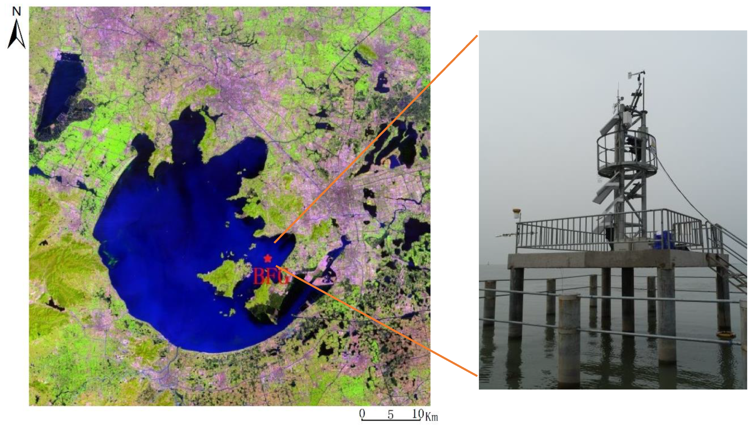
The observational data from the Bifenggang(BFG: 31°16′ N, 120°39′ E) observation platform site in eastern Lake Taihu were collected in August 2012. The site is located approximately 4 km from the eastern shore (Figure 1). An eddy covariance system was set up on the platform at a height of 8.5 m above the lake surface, consisting of a three-dimensional sonic anemometer (CSAT3, Campbell Scientific Inc., Logan, UT, USA) and an open path infrared CO2/H2O analyzer (EC150, Campbell Scientific Inc., Logan, UT, USA). The system was used to measure the three-dimensional wind speed and CO2/H2O density at a frequency of 10 Hz. Radiation data were collected by a four-component radiometer (CNR4, Kipp & Zonen B. V., Delft, The Netherlands). The air temperature, relative humidity, wind speed and wind direction were collected by a microclimate system at a height of 8.5 m above the lake (Dynakmet, Dynamax Inc., Houston, TX, USA). In addition, the water temperatures at depths of 20, 50, 100, and 150 cm and the water bottom were measured by a water thermometer (109-L, Campbell Scientific Inc., Logan, UT, USA).
The downward short-wave and downward long-wave radiation observed by the four-component radiometer and the air temperature, wind speed, wind direction, humdity obtained from the microclimate system of the BFG observation platform were used as driving data for lake models. In August 2012, there were no missing data from the microclimate station and radiation data.
Lake surface temperature, sensible heat flux and latent heat flux were used for model evaluation. The lake surface temperature was calculated by using the observed values of upward long-wave radiation according to Stephen Boltzmann’s law. Sensible heat flux and latent heat flux were not directly observed, but can be calculated from the original data of eddy correlation system after a series of processing including coordinate rotation and density correction. The missing rate of turbulence flux data in August 2012 was 7%. The missing data were interpolated with the mass transfer equation according to Xiao et al. [35]. The closure of energy balance was 71%. Detailed descriptions of the flux observation platform on Lake Taihu and the data quality control as given by Lee et al. [24], Wang et al. [36] and Xiao et al. [35].
3. Results and Discussion
3.1. Lake Surface Temperature
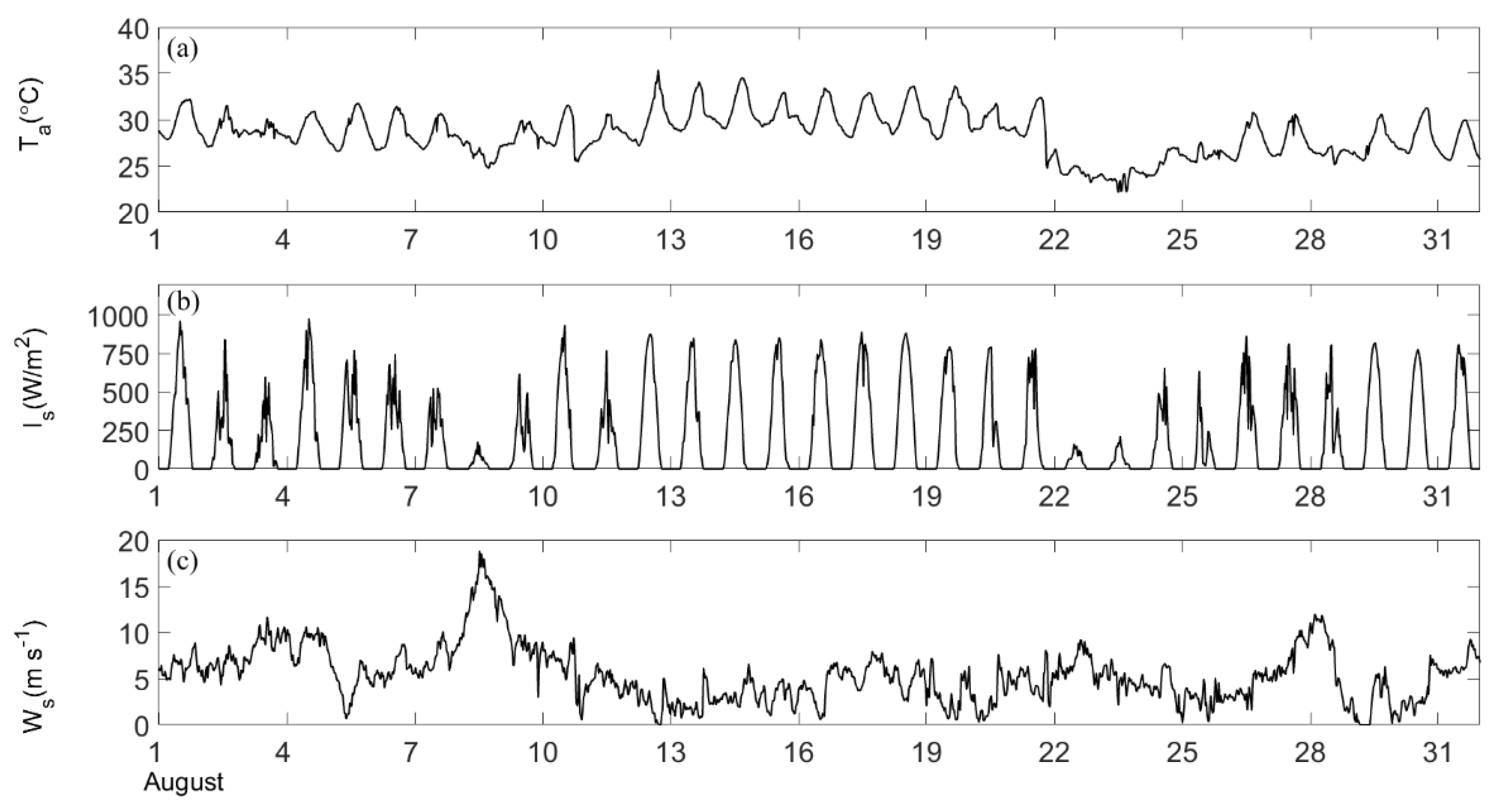
The weather conditions at the BFG site during August 2012 are shown in Figure 2. The average temperature in August was 28.5 °C, and the maximum temperature was 36.4 °C. The wind speed in August was low with an average wind speed of 5.4 m s−1. The typhoon Sura affected the area from 3 August to 4 August, and the local wind speed reached 12.8 m s−1. On 9 August, due to the typhoon Haikui, the maximum wind speed was more than 18.3 m s-1. Most of early August was cloudy, and the weather was good during most of middle and late August. The maximum solar radiation occurred at noon and was 976 W m−2.
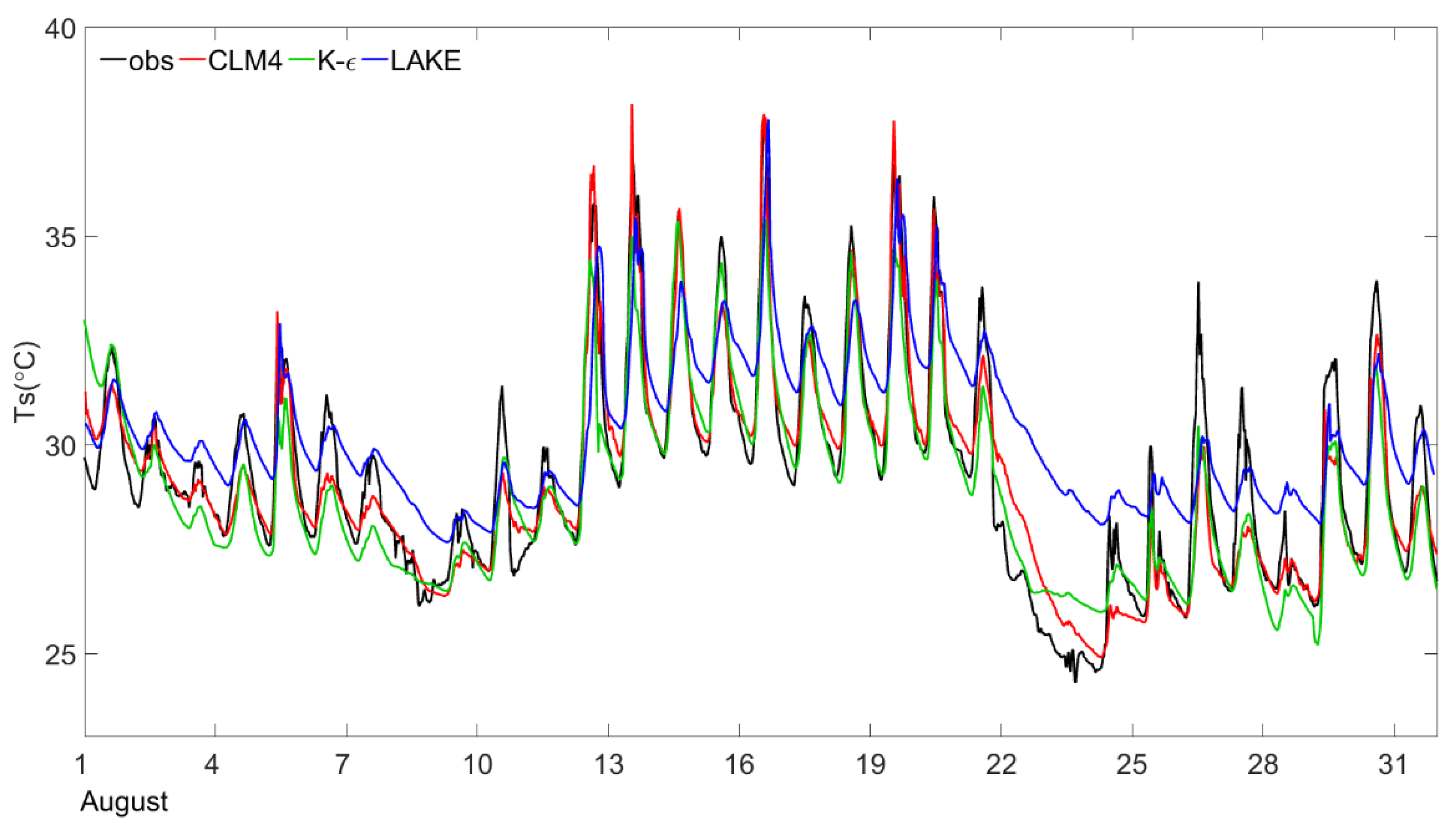
As a shallow lake, the surface temperature is greatly influenced by the weather conditions and has distinct daily variations. On clear days (e.g., 15 August 2012), the diurnal range of the lake surface temperature reached 9.2 °C (Figure 3), whereas it was relatively small (3–5 °C) on cloudy and windy days (e.g., 9 August and 28 August). The distinct diurnal variation in surface temperature caused by the weather conditions can be simulated by all of the models, and the CLM4-LISSS model yielded the best results with a correlation coefficient (CC) of 0.94 and a root mean square error (RMSE) of 0.85 °C (Table 3). The E-ε model also yielded good simulation results with a correlation CC of 0.93 and an RMSE of 0.98 °C. The results of the LAKE model had a CC of 0.82 and an RMSE of 1.45 °C, therefore it required further adjustment.
The three models used the same surface albedo, emissivity and extinction coefficient, the lake surface temperature was mainly influenced by the surface heat flux calculation scheme and the heat transferring in the water between the surface and the bottom. In August, the dense submerged plants at BFG influenced the eddy diffusion and the solar radiation transfer in the water, thus restraining the downward heat dispersion from the lake surface. In the CLM4-LISSS model, the effect of the submerged plants on turbulence is considered by decreasing the eddy diffusivity by 1.8%, which makes the simulated and observed surface temperatures consistent. However, the simulated diurnal variation of the lake surface temperature was still less than the observations, and the lower temperature at night cannot be simulated. Dale et al. [27] showed that submerged plants in lakes affect the thermal properties of the lake water, and it is possible that the overall specific heat capacity of the lake decreases when submerged plants are concentrated in the lake; this is not considered in the model, so the simulated daily range is relatively small.
The E-ε model has a more suitable design for the aquatic environment in eastern Lake Taihu because it considers the effects of extinction and fluid damping of submerged plants. The calculation of the lake surface temperature is only affected by the energy balance of the lake body and not affected by the water temperature of the sediment layer, therefore, the simulated lake surface temperature is better. However, similar to the CLM4-LISSS model, the simulated diurnal range was low.
The daily maximum lake surface temperature can be accurately simulated by the LAKE model, but the minimum temperature was overestimated, and the simulated daily variation in the surface temperature was relatively small. Moreover, the model cannot accurately simulate the response of the lake surface temperature to cooler weather. There were large differences in the lake surface temperature on 9, 23–24 and 28–29 August; on 24 August, the difference reached 4.5 °C.
3.2. The Thermal Stratification of Lake
The thermal stratification of Lake Taihu is also significantly influenced by the weather. Figure 4a shows the observed lake temperature with depth. The water temperature stratification at the BFG site was divided into three conditions: significant water temperature stratification, no stratification and weak stratification.
When wind speed is low, the water stores heat during the day, and the stratification is obvious. The thermal stratification is strong during the day due to direct heating by solar radiation. The water surface temperature is higher than the atmospheric temperature at night, and the lake surface releases heat, which weakens the thermal stratification. However, the upper water is always hotter than the lower part, and the water temperature is thermally stable for the entire day. Significant water temperature stratification occurred from 12 to 21 August. As shown in Figure 2, the temperature began to rise during this period. The daily average wind speed was only 2.8 m s−1 on 15 August. The highest lake surface temperature was 36.40 °C at 15:00, and the temperature difference between the surface and bottom reached 7.39 °C.
On cloudy days and when the wind speed was high, less heat reached the lake surface, and the strong wind strengthened the dynamic mixing of the lake body. The heat that reached the surface of the lake was rapidly transferred downward, and the water temperature became vertically uniform (3–4 August, 9 August, 23–24 August). On the days before or after a weather event, such as 1–2 August, 5 August, 7–8 August, 10 August, 21–22 August, and 25–31 August, there was low thermal stratification in the lake.
The simulations of the thermal stratification are shown in Figure 4. The downward heat mixing process during clear days could be simulated by all three models (11–21 August), and the vertically uniform water temperature stratification under mechanical mixing by strong wind (3–4 August, 9 August, and 23–24 August) was simulated by all of the models. The simulated water temperature from CLM4-LISSS (Figure 4b) is slightly higher than the observation (Figure 4a), probably because the surface energy closure hypothesis used in the model is not accurate for the real atmosphere and results in the higher simulation values. In general, the water temperature simulation is better above a depth of 1 m. In the deeper water, there are numerous submerged plants. The current scheme of CLM4-LISSS does not consider the influence of submerged plants on eddy diffusion and the storage of heat in water, so more heat is transferred downward, and the simulated water temperatures are higher than the observations. Golosoy and Kirillin [29] showed that when the heat storage of submerged plants is not considered, the simulated lake bottom water temperatures in the summer would be higher than the observations.
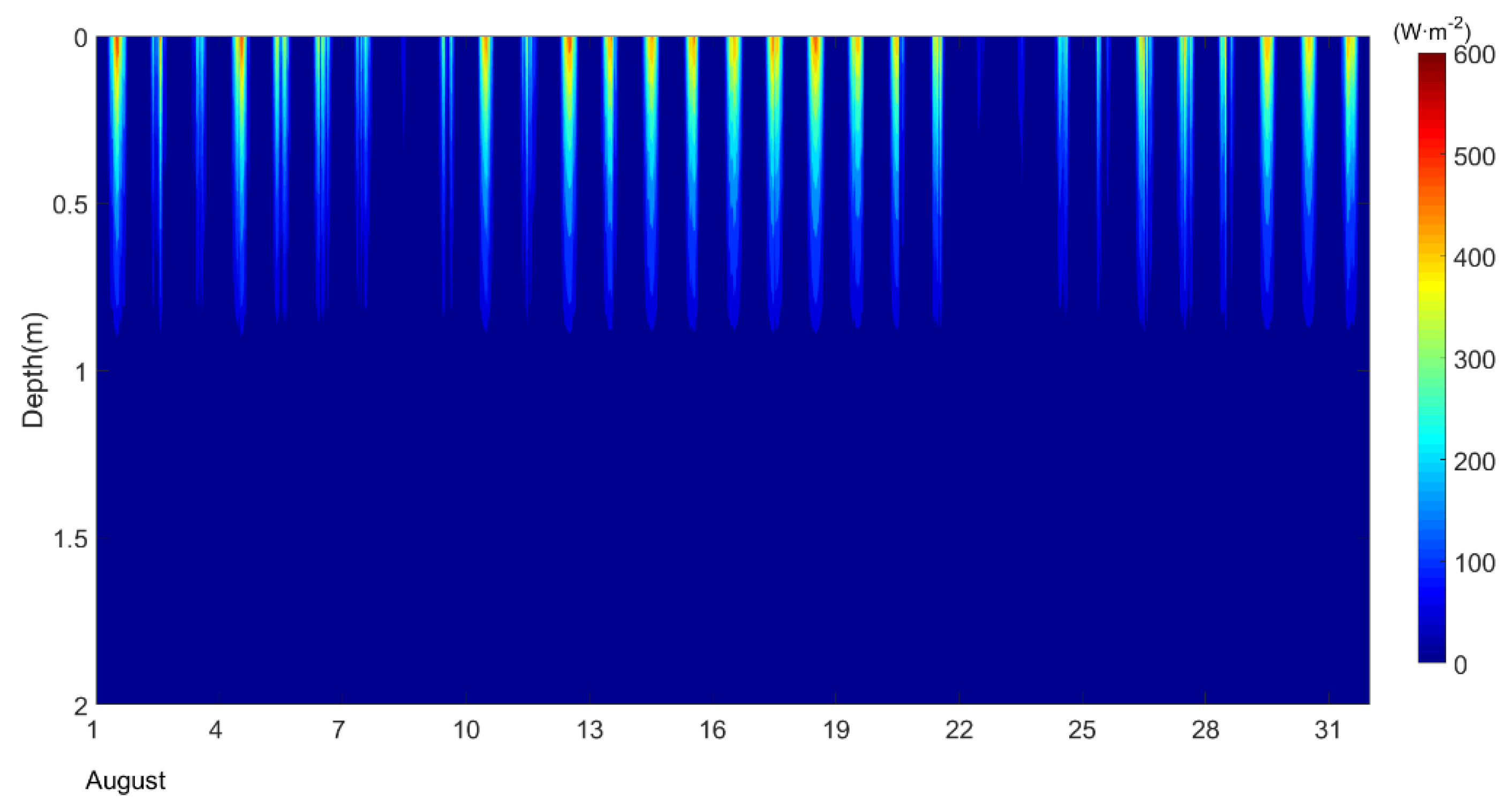
The E-ε model can accurately estimate the surface temperature but underestimates the temperature in deeper water (Table 3) because the downward heat diffusion is restrained at approximately 1 m (Figure 4c). Due to the submerged plants, it is difficult for solar radiation to reach the bottom. Figure 5 hows the solar radiation received at different water layers using the E-ε model, and the radiation was 0 at a depth of 0.8 m, which resulted in the underestimation of the water temperature in deeper layers. In addition, this model does not consider the bottom sediment effects, which should be the heat sink in the summer and not be ignored in shallow lake simulations [34].
The accuracy of the water temperature simulation by the LAKE model decreases in the lower layers of lake. At 1.5 m, the CC between the simulation and the observation decreased to 0.58 (Table 3). On clear days, the very small eddy diffusion in the upper layer only allows the heat exchange to occur in the upper layer and makes it difficult to transfer heat downward, which results in the lower water temperature at the bottom. When the wind is strong, the eddy diffusion is relatively large, which causes the overestimated water temperature at the bottom (Figure 4d).
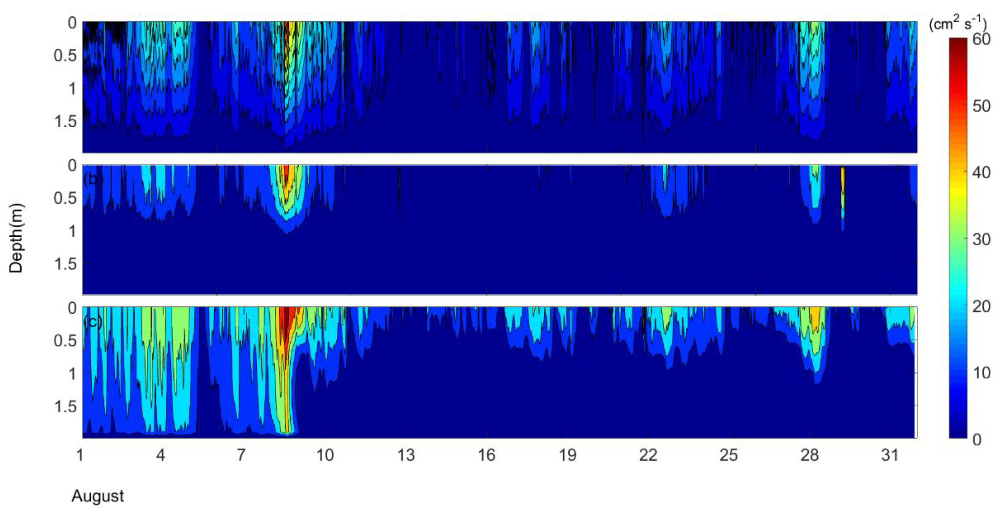
3.3. Differences in EEC and their Effects on Thermal Stratification Simulation
Water bodies are significantly different from the land. When heat enters a water body, the eddy motion has a significant impact on the thermal stratification of the water temperature. Figure 6 shows the vertical distribution of the EEC in August 2012. Deng et al. [30] indicated that the use of the 2% EEC of [32] in Lake Taihu results in the better estimations of lake temperature. The weak vertical mixing is possibly related to the low flow velocity (the time that the water remains is approximately 350 days) [37] and small ratio of depth to area. The large area (2500 km2) and shallow water (1.9 m) lead to a small depth to area ratio (0.0008) and strong resistance of the lake to the three-dimensional motion of water and turbulent mixing induced by wind. In this study, we consider the effects of submerged plants on reducing turbulence and decrease the EEC to 1.8% in the CLM4-LISSS model.
Figure 6 compares the EECs in the three model, and it can be seen that the weather conditions directly affect the distribution of the EEC in Lake Taihu. On clear days, such as 11 August to 22 August, the lake water was stable, and the EEC was low. The LAKE model simulated a stronger eddy above 50 cm that reached 30 cm2 s−1, and there was no eddy diffusion below 50 cm, resulting in little heat transfer to the deeper layers, therefore the temperature at lake bottom was significantly lower. The turbulent dissipative process in the E-ε model mainly depends on the influence of submerged plants in the water. The submerged plants in eastern Lake Taihu are higher in the summer, reaching 1.2 m, and radiation heat is stored in the lake above a depth of 1.2 m (Figure 6); this leads to a thermally stable layer, so the EEC is almost zero (Figure 4b), resulting in a higher simulated temperature in the upper layer (Figure 3). The EEC simulated by the CLM4-LISSS model is less than 10 cm2 s−1, and it can reach the deeper part of the lake. The comparison chart (Figure 3) and the statistical data (Table 3) show that the simulated water temperatures are most consistent with the observed data.
During cloudy and windy weather (4, 9 and 28 August), there was no strong radiation heat source, and the higher near surface wind drove the turbulent motion of the water body, so the turbulent mixing was greatest with the largest EEC. The maximum EEC of the CLM4-LISSS model is 46.5 cm2 s−1, that of the E-ε model is 49.7 cm2 s−1 and that of the LAKE model is 58.4 cm2 s−1. The LAKE model always yields a large EEC on these days, and the EEC simulated by the E-ε model is limited to the water body above a depth of 1.2 m, which leads to differences in the simulations of the lake temperature.
3.4. Lake Surface Energy Flux
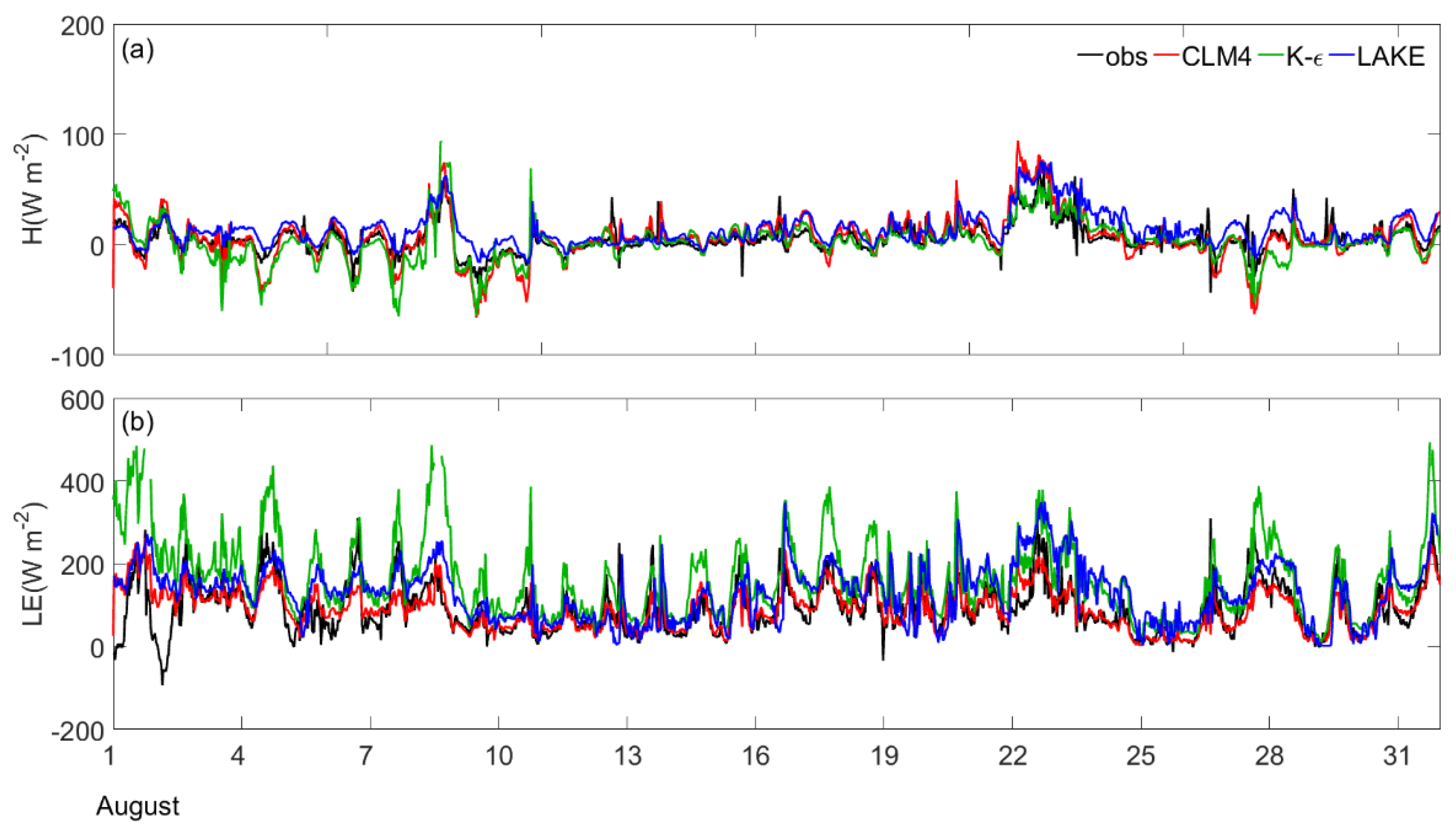
The observed sensible and latent heat fluxes are shown by the black solid lines in Figure 7. The latent heat flux dominates the lake energy distribution, when the local wind speed is high, the exchanges of latent heat and sensible heat are strong, and both the sensible heat and the latent heat flux increase substantially. For example, high near-surface wind speeds occurred on 9 August, 23 August, and 28 August (Figure 2c), and the observed latent heat flux increased significantly to a maximum of 310.6 W m−2 on 23 August (Figure 7b). During sunny weather, such as 11 August to 22 August, the radiation was strong (Figure 2b). During this period, the average wind speed was less than 5 m s−1, and the latent heat flux showed clear daily variations.
Comparisons of the simulated and observed heat fluxes every half hour are shown in Figure 7, and the CCs and RMSEs were calculated to better analyze the flux differences (Table 4). All three models can simulate the ranges of sensible heat and latent heat fluxes. When the weather is clear, the daily variation in the lake surface flux is obvious. The three models can capture the daily range of the lake surface flux. The simulation results of the CLM4-LISSS model are most consistent with the observed values on both sunny and cloudy days, with a CC of 0.78 and an RMSE of 55.32 W m−2, and the CC of the sensible heat flux was higher, reaching 0.86 (Table 4). The determination of the surface parameters in the CLM4-LISSS model is very complicated. Deng et al. [30] determined the values of the momentum, heat and water vapor roughness length based on observation data from Lake Taihu and used them in the model. By considering the Monin-Obukhov length and friction velocity under different stability conditions, the calculation scheme for the surface flux can be determined. Based on this evaluation, the scheme can be used to calculate the surface flux of Lake Taihu.
The E-ε model is better for simulating the lake surface temperature. However, the lake surface flux was calculated using an empirical function, only the temperature difference between the lake surface and the air and the wind speed were considered, and the turbulence exchange coefficient for the flux was not calculated. The simulated sensible heat flux is more consistent with the observations, although the simulated latent heat flux is significantly greater than was observed, especially under high wind speed conditions. The maximum wind speed at the surface of the lake reached 18.3 m s−1 on 9 August, and the observed maximum latent heat was 184.6 W m−2, whereas the E-ε model simulation reached 467.6 W m−2.
The formula used to calculate the surface flux in the LAKE model is similar to that in the CLM4-LISSS model. While due to the EEC bias the simulated lake surface temperature is high (Figure 8a), which results in a systematic error of the surface sensible heat flux of approximately 10 W m−2, and the simulated peak latent heat flux of the LAKE model is smaller than that of the E-ε simulation, but it is still larger than the observations, and the CC is small (Table 4).
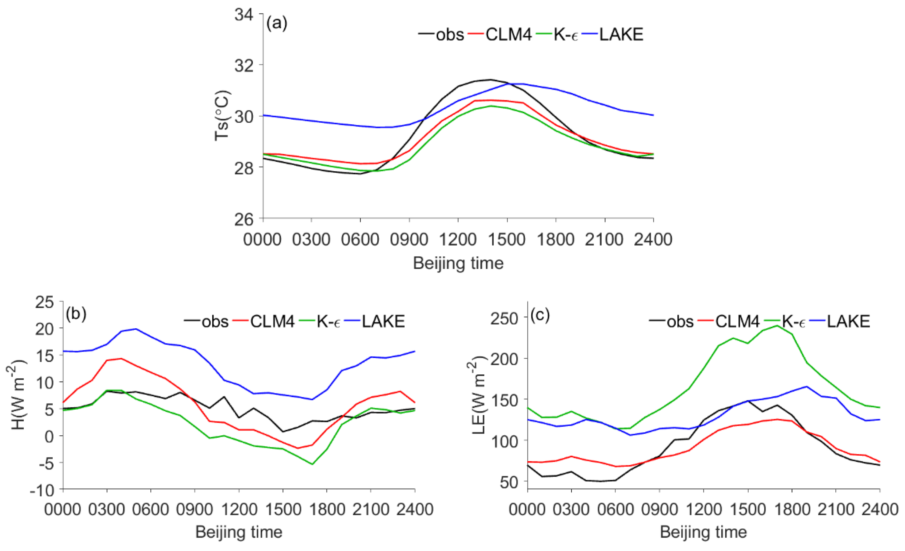
Figure 8b,c presents a comparison of the monthly average heat fluxes between the observations and simulations. The observed sensible heat flux, which is smaller during the daytime and larger at night, can be simulated well by all three models, though the simulated daily ranges are larger than the observations. The observed latent heat is high during the day and low at night and has obvious daily changes that are consistent with those of the lake surface temperature due to the stronger evaporation at higher temperatures. Even though the simulated lake surface temperature, sensible heat and latent heat of the CLM4-LISSS model are more consistent with the observed data, the sensible heat and latent heat are smaller than the observations during the day. The probable reason is the slightly lower simulated surface temperatures, which can be seen in Figure 7a. The simulated lake surface temperatures of the LAKE model are higher (Figure 7a) than the observations, and the sensible heat is significantly greater (Figure 8b). In addition, the latent heat is overestimated for the entire day. The simulated temperatures of the lake surface from the E-ε model are consistent with the observations, and the maximum value during the day is approximately 2 °C lower than the observations. However, because the empirical function depends on the wind speed on the lake, the calculated latent heat flux is much greater than the observations, and the sensible heat is smaller than the observations.
The differences between the flux simulations occur firstly because the EECs are different, which leads to differences in the lake surface temperature and further influences the heat fluxes. These were analyzed in detail in the previous sections. The momentum, heat, and water vapor roughness of the lake surface are important to the fluxes of the CLM4-LISSS and LAKE models. However, Deng et al. [30] showed that the best evaluation results of the flux observation data from Lake Taihu were obtained when these parameters were set to constants, therefore, this study used the same roughness value as in Deng et al. [30]. However, due to the differences between the water body and surfaces, the momentum, heat and water vapor roughness of the lake surface can change due to the wind and wave motion caused by the weather conditions and the local thermal circulation. However, the current application is problematic. The parameterization relationship between the wind and wave motion and roughness is not clear. Moreover, even though CLM4-LISSS provides better simulation results, the bottom water temperature is still overestimated because the effects of submerged plants on heat storage, conduction and eddy diffusion are not considered.
In addition, because the BFG observation site is relatively close to the shore, it is affected by urban heat islands circulation and the local lake breeze. The existence of these local circulations and the effects of geostrophic wind under different weather conditions may have large impacts on the surface heat transport of lakes, which may cause the lake surface energy exchange to not be closed, whereas the model was developed based on the assumption of energy closure, which would influence the simulation results. Figure 9 shows the diurnal variations of the monthly averages of the surface energy components in August, where Qg is the heat transfer from the surface layer to the lake, (1 − β) Rs is the heat storage at the surface layer of the lake, β is the proportion of the heat entering the water, and the sum of Qg and (1 − β) Rs is the heat storage Q in the water. Due to the use of the same extinction coefficient in the three models, there is no difference in the downward heat transfer ((1 − β) Rs) between the models, but there is a difference in the heat transfer from the lake surface layer to the lake water because it is related to the water temperature. Due to the small proportion of sensible heat flux in the total energy, the differences between the simulations and observations of the sensible heat flux are also small, and the simulated latent heat flux is slightly greater than the observations. Wang et al. [36] showed that the monthly average of the closure of the energy balance in the Lake Taihu area is 71%, which may be the potential cause of the simulation results being greater than the observed data.
4. Conclusions and Discussion
In this paper, three lake models were used to simulate the lake-air exchange in the submerged plant area of eastern Lake Taihu in August 2012. The characteristics of the thermal stratification and the effect of the EEC of the lake body on the water temperature were analyzed.
Lake Taihu is a shallow lake, and the thermal stratification is significantly influenced by the weather conditions. On sunny days, the lake is thermally stable, with the maximum daily diurnal range of the lake surface temperature reaching 8.2 °C and the maximum temperature difference between the lake surface and the bottom reaching 7.39 °C. On cloudy days, few heat accumulates in the lake, the strong wind causes eddy motion in the water body, and the heat transferring increases, so the structure of thermal stratification is not obvious.
The three models (CLM4-LISSS, E-ε and LAKE) can simulate the diurnal variation in the lake surface temperature in August 2012. The CLM4-LISSS model gives the best simulation results with a CC of 0.94 and an RMSE of 0.85 °C. The main differences are the higher surface temperatures at night. In addition, because the lower layer of the model does not consider the influence of submerged plants, more heat is diffused downward, so there are some deviations. The E-ε model produces a better simulation than the LAKE model; the CC is 0.93, and the RMSE is 0.98 °C. However, the performance of the E-ε model decreases in the deep water. The water temperature at the bottom is underestimated because the submerged plants restrain the radiation transfer to the deep water and reduce it to 0 at a depth of 1 m, so it is difficult to heat the water in the lower layers. Moreover, because of the dissipative effect of submerged plants on eddy flow, the EEC in the water body at a depth of 1.2 m and below is nearly 0, and the heat cannot transfer to the lower layers. A comparison of the EECs shows that the EEC of the LAKE model is too high in the windy days. As a result, the transferring of heat increases, and the temperature stratification decreases, and in sunny days for the eddy diffusivity remains in upper layer of the water and the heat is hard to transfer downward.
The results of this study indicate that the latent heat flux in the three models can simulate the daily variation in the lake surface flux, but all of the models overestimated the latent heat flux to some extent, probably because the observed energy balance is not closed. The CLM4-LISSS model provides a more comprehensive consideration of the latent heat flux calculation and thus obtains better simulation results. The E-ε model overestimates the latent heat flux because it uses an empirical function that depends on the local wind speed to calculate the flux. The LAKE model has higher sensible heat and latent heat than the observations due to the overestimated surface temperature.
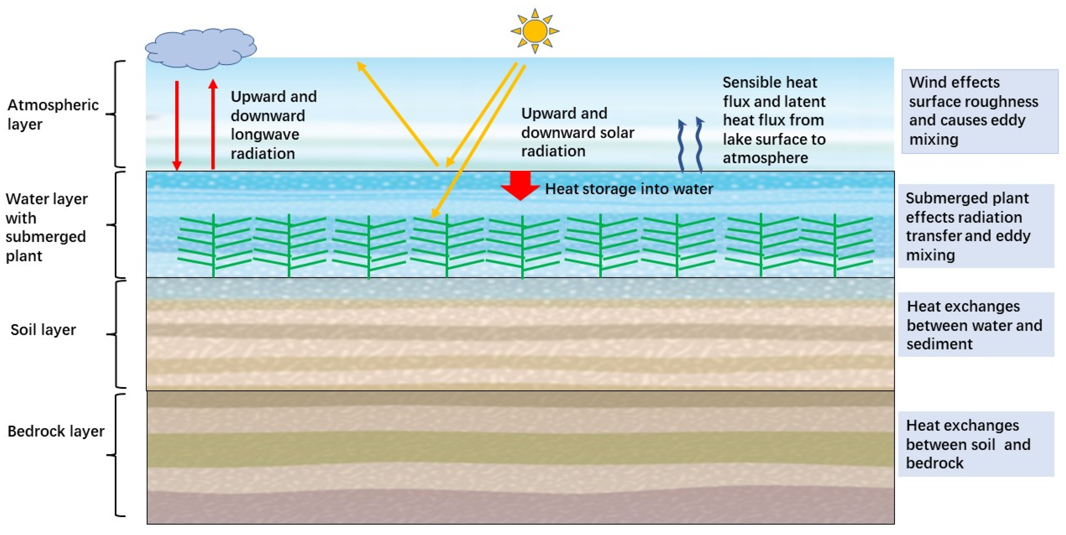
This study indicates that the model suitable for Lake Taihu still need to be developed based on the current models. Figure 10 presents the framework of the new model. The calculation of the surface flux of the lake is better when the Monin-Obukhov theory is used and the accurate EEC scheme is important for simulating the lake-air exchange. A roughness parameterization scheme that is suitable for shallow lakes and is able to describe the interaction between wind and waves needs to be developed further. How to reasonably describe the influence of submerged plants on the thermal stratification of shallow lakes requires careful consideration. In addition, for the shallow lake model, the heat exchange between water and sediment can’t be ignored. This paper uses the observations at a single site to evaluate different lake models. Eight years of data are available from five different sites on Lake Taihu. These data will be used to evaluate the models to reduce the temporal and spatial effects on simulations by different models.
The 1-D model was used to simulate the area with dense submerged plants in Lake Taihu in this paper. The current model ignores the effect of horizontal movement of water on heat transfer. The water flow in this region is relatively slow due to the influence of submerged plants. Therefore, the simulation results based on the 1-D model were in good agreement with the single site observations. However, it is very important to develop 3-D models that consider the movement of water and the horizontal heterogeneity of the physical characteristics of lake body when simulating the lake-air exchange of the entire lake. At present, the rapidly increased speed of supercomputers is also helpful to the realization of this work.
Author Contributions
Conceptualization, Y.W. and S.L.; methodology, Y.W.; software, Y.G.; validation, Q.M.; X.H.; formal analysis, Q.M.; data curation, Q.M.; writing—original draft preparation, Y.W.; writing—review and editing, S.L.; project administration, Y.W.; funding acquisition, Y.W.
Funding
This research was funded by the National Natural Science Foundation of China, grant number 41275024, and the sponsorship of Jiangsu oversea Visiting Scholar Program for University Prominent Youth & Middle-aged Teachers and Presidents.
Acknowledgments
Sincerely thank the reviewers for their comments, which is of great help to the improvement of this paper.
Conflicts of Interest
The authors declare no conflict of interest.
References
- Sun, S.F.; Yan, J.F.; Xia, N.; Li, Q. The model study of water mass and energy exchange between the inland water body and atmosphere. Sci. China Ser. G Phys. Mech. Astron. 2008, 51, 1010–1021. [Google Scholar] [CrossRef]
- Sun, S.F.; Yan, J.F.; Xia, N.; Sun, C.H. Development of a model for water and heat exchange between the atmosphere and a water body. Adv. Atmos. Sci. 2007, 24, 927–938. [Google Scholar] [CrossRef]
- Adrian, R.; Reilly, C.M.O.; Zagarese, H.; Baines, S.B.; Hessen, D.O.; Keller, W.; Livingstone, D.M.; Sommaruga, R.; Straile, D.; Van, D.E.; et al. Lakes as sentinels of climate change. Limnol. Oceanogr. 2009, 54, 2283–2297. [Google Scholar] [CrossRef] [PubMed]
- Long, Z.; Perrie, W.; Gyakum, J.; Caya, D.; Laprise, R. Northern lake impacts on local seasonal climate. J. Hydrometeorol. 2007, 8, 881–896. [Google Scholar] [CrossRef]
- Butcher, J.B.; Nover, D.; Johnson, T.E.; Clark, C.M. Sensitivity of lake thermal and mixing dynamics to climate change. Clim. Chang. 2015, 129, 295–305. [Google Scholar] [CrossRef]
- Goyal, M.K.; Ojha, C.S.P. Evaluation of Rule and Decision Tree Induction Algorithms for Generating Climate Change Scenarios for Temperature and Pan Evaporation on a Lake Basin. J. Hydrol. Eng. 2013, 19, 828–835. [Google Scholar] [CrossRef]
- Lyons, W.A. The climatology and prediction of the Chicago lake breeze. J. Appl. Meteorol. 1972, 11, 1259–1270. [Google Scholar] [CrossRef]
- Zhang, L.; Zhu, B.; Gao, J.H.; Kang, H.Q. Impact of Taihu Lake on city ozone in the Yangtze River Delta. Adv. Atmos. Sci. 2017, 34, 226–234. [Google Scholar] [CrossRef]
- Mironov, D.; Heise, E.; Kourzeneva, E. Implementation of the lake parameterisation scheme FLake into the numerical weather prediction model COSMO. Boreal Environ. Res. 2010, 15, 218–230. [Google Scholar]
- Hostetler, S.W.; Bartlein, P.J. Simulation of lake evaporation with application to modeling lake level variations of harney-malheur lake, Oregon. Water Resour. Res. 1990, 26, 2603–2612. [Google Scholar]
- Fang, X.; Stefan, H.G. Long-term lake water temperature and ice cover simulations/measurements. Cold Reg. Sci. Technol. 1996, 24, 289–304. [Google Scholar] [CrossRef]
- Subin, Z.M.; Riley, W.J.; Mironov, D. An improved lake model for climate simulations: Model structure, evaluation, and sensitivity analyses in CESM1. J. Adv. Modeling Earth Syst. 2012, 4. [Google Scholar] [CrossRef]
- Ren, X.Q.; Li, Q.; Chen, W.; Liu, H.Z. A new lake-gas heat transfer model and its simulation capability evaluation. Adv. Atmos. Sci. 2014, 38, 993–1004. (In Chinese) [Google Scholar]
- Yeates, P.S.; Imberger, J. Pseudo two-dimensional simulations of internal and boundary fluxes in stratified lakes and reservoirs. Int. J. River Basin Manag. 2003, 1, 297–319. [Google Scholar] [CrossRef]
- Goudsmit, G.H.; Burchard, H.; Peeters, F. Application of k-ε turbulence models to enclosed basins: The role of internal seiches. J. Geophys. Res. Ocean. 2002, 107. [Google Scholar] [CrossRef]
- Stepanenko, V.M.; Lykossov, V.N. Numerical modeling of heat and moisture transfer processes in a system lake—Soil. J. Russ. Meteorol. Hydrol. 2005, 3, 95–104. [Google Scholar]
- Stepanenko, V.; Joehnk, K.D.; Machulskaya, E.; Perroud, M.; Subin, Z.; Nordbo, A.; Mammarella, I.; Mironov, D. Simulation of surface energy fluxes and stratification of a small boreal lake by a set of one-dimensional models. Tellus 2014, 66, 174–179. [Google Scholar] [CrossRef]
- Thiery, W.; Stepanenko, V.M.; Fang, X.; JӧHnk, K.D.; Li, Z.; Martynov, A.; Perroud, M.; Subin, Z.M.; Darchambeau, F.; Mironov, D.; et al. LakeMIP Kivu: Evaluating the representation of a large, deep tropical lake by a set of one-dimensional lake models. J. Tellus A Dyn. Meteorol. Oceanogr. 2014, 68, 21390. [Google Scholar] [CrossRef]
- Ren, X.Q.; Sun, S.F.; Chen, W.; Liu, H.Z. Summary of current research on numerical simulation of lakes. Adv. Earth Sci. 2013, 28, 347–356. (In Chinese) [Google Scholar]
- Gu, H.P.; Jin, J.M.; Wu, Y.H.; Ek, M.B.; Subin, Z.M. Calibration and validation of lake surface temperature simulations with the coupled wrf-lake model. Clim. Chang. 2015, 129, 471–483. [Google Scholar] [CrossRef]
- Xu, L.J.; Liu, H.Z.; Du, Q.; Wang, L. Evaluation of the WRF-lake model over a highland freshwater lake in southwest China. J. Geophys. Res. Atmos. 2016, 121, 13989–14005. [Google Scholar] [CrossRef]
- Heiskanen, J.J.; Mammarella, I.; Ojala, A.; Stepanenko, V.; Erkkilä, K.M.; Miettinen, H.; Sandstrӧm, H.; Eugster, W.; Leppäranta, M.; Järvinen, H.; et al. Effects of water clarity on lake stratification and lake-atmosphere heat exchange. J. Geophys. Res. Atmos. 2015, 120, 7412–7428. [Google Scholar] [CrossRef]
- Zolfaghari, K.; Duguay, C.R.; Pour, H.K. Satellite-derived light extinction coefficient and its impact on thermal structure simulations in a 1-D lake model. Hydrol. Earth Syst. Sci. 2017, 21, 377–391. [Google Scholar] [CrossRef]
- Lee, X.H.; Liu, S.D.; Xiao, W.; Wang, W.; Gao, Z.Q.; Cao, C.; Hu, C.; Hu, Z.H.; Shen, S.H.; Wang, Y.W. The Taihu eddy flux network: an observational program on energy, water, and greenhouse gas fluxes of a large freshwater lake. Bull. Am. Meteorol. Soc. 2014, 95, 1583–1594. [Google Scholar] [CrossRef]
- Yang, Y.C.; Wang, Y.W.; Zhang, Z.; Wang, W.; Ren, X.; Gao, Y.Q.; Liu, S.D.; Lee, X.H. Diurnal and Seasonal Variations of Thermal Stratification and Vertical Mixing in a Shallow Fresh Water Lake. J. Meteorol. Res. 2018, 32, 219–232. [Google Scholar] [CrossRef]
- Horppila, J.; Nurminen, L. Effects of submerged macrophytes on sediment resuspension and internal phosphorus loading in lake hiidenvesi (southern Finland). Water Res. 2003, 37, 4468–4474. [Google Scholar] [CrossRef]
- Dale, H.M.; Gillespie, T.J. The influence of submersed aquatic plants on temperature gradients in shallow water bodies. Botany 1977, 55, 2216–2225. [Google Scholar] [CrossRef]
- Fang, X.; Stefan, H.G. Dynamics of heat exchange between sediment and water in a lake. Water Resour. Res. 1996, 32, 1719–1727. [Google Scholar] [CrossRef]
- Golosov, S.; Kirillin, G.A. parameterized model of heat storage by lake sediments. Environ. Model. Softw. 2010, 25, 793–801. [Google Scholar] [CrossRef]
- Deng, B.; Liu, S.D.; Xiao, W.; Wang, W.; Jin, J.M.; Lee, X.H. Evaluation of the clm4 lake model at a large and shallow freshwater lake*. J. Hydrometeorol. 2013, 14, 636–649. [Google Scholar] [CrossRef]
- Cheng, X.; Wang, Y.W.; Hu, C.; Wang, W.; Zhang, N.; Xiao, Q.T.; Liu, S.D.; Lee, X.H. The lake-air exchange simulation of a lake model over eastern Taihu Lake based on the E-ε turbulent kinetic energy closure thermodynamic process. Acta Meteorol. Sin. 2016, 74, 633–645. (In Chinese) [Google Scholar]
- Henderson-Sellers, B. New formulation of eddy diffusion thermocline models. J. Appl. Math. Model. 1985, 9, 441–446. [Google Scholar] [CrossRef]
- Herb, W.R.; Stefan, H.G. Dynamics of vertical mixing in a shallow lake with submersed macrophytes. Water Resour. Res. 2005, 41, 293–307. [Google Scholar] [CrossRef]
- Stepanenko, V.M.; Martynov, A.; Jӧhnk, K.D.; Subin, Z.M.; Perroud, M.; Fang, X.; Beyrich, F.; Mironov, D.; Goyette, S. A one-dimensional model intercomparison study of thermal regime of a shallow, turbid midlatitude lake. J. Geosci. Model Dev. 2013, 6, 1337–1352. [Google Scholar] [CrossRef]
- Xiao, W.; Liu, S.D.; Wang, W.; Yang, D.; Xu, J.P.; Cao, C.; Li, H.C.; Lee, X.H. Transfer coefficients of momentum, sensible heat and water vapour in the atmospheric surface layer of a large freshwater lake. Bound-Lay. Meteorol. 2013, 148, 479–494. [Google Scholar] [CrossRef]
- Wang, W.; Xiao, W.; Cao, C.; Gao, Z.Q.; Hu, Z.H.; Liu, S.D.; Shen, S.H.; Wang, L.L.; Xiao, Q.T.; Xu, J.P. Temporal and spatial variations in radiation and energy balance across a large freshwater lake in China. J. Hydrol. 2014, 511, 811–824. [Google Scholar] [CrossRef]
- Shu, Q.A. The human-induced driver on the development of Lake Taihu. In Proceedings of the Conference on the 93rd ESA Annual Meeting, San Jose, CA, USA, 3–8 August 2008. [Google Scholar]
Figure 1.
Locations of Lake Taihu and observation platform, BFG.

Figure 2.
Weather conditions at BFG Station in Lake Taihu in August 2012. (a) is 2m air temperature, (b) is downward solar radiation and (c) is 10m wind speed.
Figure 2.
Weather conditions at BFG Station in Lake Taihu in August 2012. (a) is 2m air temperature, (b) is downward solar radiation and (c) is 10m wind speed.

Figure 3.
Simulation of lake surface temperature at the BFG site of Taihu Lake in August 2012.

Figure 4.
Simulation of vertical temperature profile (lake stratification) in the August 2012 at BFG station in Lake Taihu (a) Observations, (b) CLM4-LISSS, (c) E-ε, (d)LAKE.
Figure 4.
Simulation of vertical temperature profile (lake stratification) in the August 2012 at BFG station in Lake Taihu (a) Observations, (b) CLM4-LISSS, (c) E-ε, (d)LAKE.

Figure 5.
Solar radiation received at different lake depths in the E-ε model.

Figure 6.
Vertical variations of eddy diffusivity coefficients of lake models (a) CLM4-LISSS, (b) E-ε (c) LAKE.
Figure 6.
Vertical variations of eddy diffusivity coefficients of lake models (a) CLM4-LISSS, (b) E-ε (c) LAKE.

Figure 7.
Simulations and observations of the sensible heat flux (a) and latent heat flux (b) at lake surface every half hour in Lake Taihu in August 2012.
Figure 7.
Simulations and observations of the sensible heat flux (a) and latent heat flux (b) at lake surface every half hour in Lake Taihu in August 2012.

Figure 8.
Comparison of simulated and observed diurnal variations of monthly mean surface temperature(a), Sensible heat (b) and latent heat (c).
Figure 8.
Comparison of simulated and observed diurnal variations of monthly mean surface temperature(a), Sensible heat (b) and latent heat (c).

Figure 9.
Simulation and observation of average monthly variation of lake surface layer energy in Taihu in August 2012. Rs is net radiation flux, L is downward long-wave radiation, L is upward long-wave radiation, and LE is latent heat Flux, H is the sensible heat flux, Qg refers to the heat transfer from the surface layer to the lake, and (1 − β) Rs refers to the heat storage in the surface layer of the lake.

Figure 10.
The framework of the proposed lake model.


Table 1.
Comparison of physical processes in three lake models.
| Lake Type | Vertical Stratification/Layers | Parameterization Scheme of Eddy Flux between Lake and Atmosphere | Parameterization Scheme of EEC | Consideration of Sediment Layers |
|---|---|---|---|---|
| CLM4-LISSS | multilayer/10 layers | Monin-Obukhov Similarity Theory | Henderson–Sellers scheme [32] | Yes |
| E-ε lake model | multilayer/50 layers | Empirical function | Eddy kinetic energy prediction equations | No |
| LAKE | multilayer/10 layers | Monin-Obukhov Similarity Theory | Eddy kinetic energy and dissipation prediction equations | Yes |
Table 2.
The parameters used in the evaluation of the three models.
| CLM4–LISSS | E–ε Lake Model | LAKE | |
|---|---|---|---|
| Lake surface albedo | 0.055 | 0.055 | 0.055 |
| Extinction coefficient of water turbidity | 5 m−1 | 5 m−1 | 5 m−1 |
| Extinction coefficient of submerged plant | — | 0.02 m2 gdw−1 | — |
| EEC | k: Karman constant : surface friction velocity z: layer depth of lake p0: neutral value of turbulent Prandtl number ri: Richardson number N: Brunt-Vaisala constant | , set to be 0.1 mixing length coefficient turbulent kinetic energy. | λ0: molecular diffusivity V: wind speed V0: wind speed at which eddy diffusivity reaches its maximum λmax = 150 W (m K)−1 |
| Macrophyte height | — | 1.2m | — |
| Macrophyte biomass density | — | 100 gdw m−3 | — |
Table 3.
Statistical analysis of simulated and observed values in different layers of lake water temperature in Taihu in August 2012.
Table 3.
Statistical analysis of simulated and observed values in different layers of lake water temperature in Taihu in August 2012.
| CC | Centralized RMSE (°C) | |||||||||
|---|---|---|---|---|---|---|---|---|---|---|
| TS | TW (20 cm) | TW (50 cm) | TW (100 cm) | TW (150 cm) | TS | TW (20 cm) | TW (50 cm) | TW (100 cm) | TW (150 cm) | |
| CLM4 | 0.94 | 0.94 | 0.94 | 0.96 | 0.95 | 0.85 | 0.64 | 0.59 | 0.42 | 0.53 |
| E-ε | 0.93 | 0.93 | 0.92 | 0.90 | 0.8 | 0.98 | 0.68 | 0.66 | 0.65 | 1.03 |
| LAKE | 0.82 | 0.93 | 0.89 | 0.58 | 0.06 | 1.45 | 0.64 | 0.78 | 1.20 | 1.49 |
Table 4.
Statistical values of simulation and observation of surface heat flux in Lake Taihu in August 2012.
Table 4.
Statistical values of simulation and observation of surface heat flux in Lake Taihu in August 2012.
| CC | Centralized RMSE (W m−2) | |||
|---|---|---|---|---|
| H | LE | H | LE | |
| CLM4 | 0.86 | 0.78 | 11.61 | 55.32 |
| E-ε | 0.77 | 0.72 | 11.56 | 64.53 |
| LAKE | 0.71 | 0.55 | 10.96 | 61.96 |
© 2019 by the authors. Licensee MDPI, Basel, Switzerland. This article is an open access article distributed under the terms and conditions of the Creative Commons Attribution (CC BY) license (http://creativecommons.org/licenses/by/4.0/).
Share and Cite
MDPI and ACS Style
Wang, Y.; Ma, Q.; Gao, Y.; Hao, X.; Liu, S. Simulation of the Surface Energy Flux and Thermal Stratification of Lake Taihu with Three 1-D Models. Water 2019, 11, 1026. https://doi.org/10.3390/w11051026
AMA Style
Wang Y, Ma Q, Gao Y, Hao X, Liu S. Simulation of the Surface Energy Flux and Thermal Stratification of Lake Taihu with Three 1-D Models. Water. 2019; 11(5):1026. https://doi.org/10.3390/w11051026
Chicago/Turabian StyleWang, Yongwei, Qian Ma, Yaqi Gao, Xiaolong Hao, and Shoudong Liu. 2019. "Simulation of the Surface Energy Flux and Thermal Stratification of Lake Taihu with Three 1-D Models" Water 11, no. 5: 1026. https://doi.org/10.3390/w11051026
Note that from the first issue of 2016, this journal uses article numbers instead of page numbers. See further details here.