Article

Assessing Hydrological Effects of Bioretention Cells for Urban Stormwater Runoff in Response to Climatic Changes

1
School of Architecture, Southeast University, Nanjing 210096, China
2
College of Architecture and Urban Planning, Guangzhou University, Guangzhou 510006, China
3
Biophilic lab, Z+T Studio, Shanghai 200052, China
4
Nanyang Environment & Water Research Institute, Nanyang Technological University, Singapore 637141, Singapore
5
School of Civil Engineering, Guangzhou University, Guangzhou 510006, China
6
Faculty of Built Environment, University of New South Wales, Sydney, NSW 2052, Australia
7
School of Civil and Environmental Engineering, Nanyang Technological University, Singapore 639798, Singapore
*
Authors to whom correspondence should be addressed.
Water 2019, 11(5), 997; https://doi.org/10.3390/w11050997
Submission received: 31 March 2019 / Revised: 24 April 2019 / Accepted: 9 May 2019 / Published: 13 May 2019
(This article belongs to the Special Issue Urban Rainfall Analysis and Flood Management)

Abstract

:
An investigation into the effectiveness of bioretention cells (BCs) under potential climatic changes was conducted using representative concentration pathways. A case study of Guangzhou showed changes in peak runoff in climate change scenarios, with obvious growth in RCP8.5 and slight growth in RCP2.6. The performance of BCs on multiple parameters, including reduction of runoff volume, peak runoff, and first flush, were examined in different design storms using a hydrology model (SWMM). The effectiveness of BCs varied non-linearly with scale. Their performance fell by varying amounts in the various scenarios. BCs could provide sufficient effects in response to short-return-period and short-duration storms, but the performance of BCs decreased with heavy storms, especially considering climate change. Hence, BCs cannot replace grey infrastructure but should be integrated with them. The method developed in this study could be useful in the planning and design of low impact development in view of future climate changes.

1. Introduction

Global warming due to increasing atmospheric concentrations of greenhouse gasses may cause significant changes in the frequency and patterns of storms [1]. More frequent storms may cause serious problems, especially in high-density urban areas [2]. Consequently, projections of climate change play a fundamental role in risk assessment of extreme storms. A number of studies based on climate scenario modeling have investigated the impacts on rainfall patterns [3,4]. Moss et al. [5] developed the “parallel” approach, including representative concentration pathways (RCPs), which reflects different possible futures based on climate forcing, offering an important base for climatic change projection [6]. Fix et al. [7] projected that precipitation extremes will increase over the contiguous United States between 2005 and 2080 under RCP8.5 and RCP4.5. Bacmeister et al. [8] projected that extreme storms will become more common under future warming scenarios. Recently, the Scenario Model Intercomparison Project (ScenarioMIP) provided multi-model climate scenarios to simulate the variation of rainfall patterns in accordance with warming scenarios regarding RCPs and other possibilities of shared socio-economic pathways [9]. Such projections could provide valuable inputs for better understanding the adaptation and/or mitigation measures necessary to respond to the potential uncertainty from climate change.
Low impact development (LID) using decentralized designs to control stormwater runoff in response to the costly economic and unfavorable environmental impacts of conventional drainage practices has become highly attractive method for restoring predevelopment hydrological processes by prompting infiltration, detention, and adsorption [10]. As a popular LID practice, bioretention cells (BCs) with shallow depressions have been implemented to combat runoff from small-scale catchments (usually less than 2 ha), for multiple hydro-environmental benefits, such as reducing runoff volume, peak flow, and pollutant loads [11,12]. A growing number of studies have evaluated the hydrological performance of BCs using field and laboratory experiments [13,14,15,16,17], as well as hydrological and hydraulic models [18,19].
Obviously, the hydrological performance of BCs is highly sensitive to their structure and scale, as well as to external catchments and rainfall events, so it is necessary to adjust their construction to all these parameters. For flooding mitigation, Winston et al. [20] showed that the runoff from regular rainfall can be controlled, and the initial part of surface runoff from storms can be retained, by enough storage volumes of BCs. In addition, Baek et al. [21] found that the first flush effect—high concentration of contamination in the initial portion of surface runoff—could be effectively reduced with enough retention space in BCs. Also, many studies have found that BCs can effectively mitigate peak runoff in various rainfall events [22,23,24]. Thus, it is necessary to identify suitable scales and parameters of BCs to account for targets of runoff quantity and quality management and to maximize life-cycle performance.
Climate change is a dynamic factor, making stormwater management very difficult to plan for. However, there is some information on optimizing the hydrological cost-effectiveness of LID practices, including BCs, in response to the uncertainty of climate change. Hathaway et al. [25] found that BCs could be provided to adapt to the uncertainty based on climate scenarios in North Carolina, USA. Zahmatkesh et al. [26] assessed the effect of BCs on urban storm runoff in response to climate changes in New York. Borris et al. [27] investigated runoff quality with control of BCs under climatic changes in urban and suburban catchments of Ostersund, Sweden. There is potential for BCs to be used as resilient landscape to mitigate some of the adverse influences of climate change on urban hydrology. In addition, there are still opportunities for further advancement of our knowledge of the hydro-environmental performance of BCs under climate change in terms of the reduction of runoff volume, peak flow, and first flush.
The objectives of this study are: (1) to analyze the possible influence of climate change on storm runoff in urban catchments; (2) to assess the hydrological performance of BCs under climate change; and (3) to examine the targeted scale of BCs to meet different hydro-interests based on climate scenarios. The methodology developed here could be applied to develop options for LID as adaptation/mitigation measures for climate change under local conditions.

2. Methodology

Climate scenarios were simulated to examine their impacts on surface runoff in a hypothetical urban catchment through alteration of storms. Then, hydro-modeling simulation was used to assess the hydro-environmental benefits of BCs in different climate scenarios. Finally, the targeted scales of BCs to meet different performance interests (in response to the uncertainty of future changes) were derived (Figure 1).

2.1. Study Site

Guangzhou, China (22°95’ N; 113°35’ E), a high-density, subtropical city with around 1600 mm of annual precipitation and 77% relative humidity, is located in the south of China. The urban areas in Guangzhou are seriously threatened by waterlogging due to the uneven spatiotemporal distribution of rainfall events [28]. From 2009 to 2015, there were 739 flooding hotspots and 1908 urban flooding events in Guangzhou [29]. In addition, Zhao et al. [30] analyzed the spatial and temporal changes of precipitation extremes and found that daily intensity shows a significant positive trend in Guangzhou. Zhang et al. [31] projected an increase in extreme storms in Guangzhou in 2020–2050, compared to 1970–2000, using climate models and emissions scenarios.
Due to their flexibility of scale, BCs’ positive life-cycle benefits can be effectively integrated into dense urban areas [32,33,34]. BCs have been widely applied in urban areas through strong support from local governments, such as in the Sponge City program [35]. It is critical to develop a comprehensive approach to support effective BCs adoption in Guangzhou in response to climate change.
A hypothetical urban catchment is chosen in Guangzhou as a case study. The catchment was assumed to be rather flat (average slope 1%), small (5000 m2), and 50% impervious (Table 1). BCs were assumed to be located in the low-point area of this catchment and all surface runoff from the impervious and pervious area of catchment was discharged to BCs. In addition, there is no pipe network in this catchment. Climate scenarios were compared to current conditions as a baseline. Depending on the management targets, various design storms (different intensities and durations) need to be simulated. The design storms were clustered into six groups based on representative return period (P) (1, 10, and 100 year) and durations of storms (1 h and 6 h). The local storm intensity distribution for Guangzhou is as shown in Equation (1).
i = a ( t + b ) c = A ( 1 + C log P ) 167 × ( t + b ) c = 14.52   ( 1 + 0.533 × lg P ) ( t + 11 ) 0.668
where i is the storm intensity (mm/min), P is the return period (year), and t is rainfall duration (h); as well as a (rain force parameter), b, c, A are the parameters in Guangzhou. a = 14.52   ( 1 + 0.533 × lg P ), b = 11, c = 0.668, and A = 2424.17.
Chicago hyetograph model, closest to the actual rainfall pattern, is well defined and widely used to represent synthetic rainfalls [36]. The formulae for synthetic Chicago storms, used to quantify the rainfall patterns, are
i ( t b ) = a [ ( 1 c ) × t b r + b ] ( t b r + b ) 1 + c
and
i ( t a ) = a [ ( 1 c ) × t a 1 r + b ] ( t a 1 r + b ) 1 + c
where i ( t a ) and i ( t b ) are the storm intensity (mm/min) after and before the peak time point respectively; the parameter r refers to the time-to-peak factor. According to previous studies [37,38], this value ranges from 0–1 of the storm duration, and a reasonable range for r is 0.3–0.5. Short of any other information available, a value of 0.5 was chosen in this study. Here, a, b, and c are parameters from Equation (1).

2.2. Climate Scenarios

Climate change scenarios, describing potential developments of anthropogenic climate change in the future, facilitate identifying the effectiveness of different adaptation and/or mitigation strategies [41]. In this study, four RCPs including 2.6, 4.5, 6.0, and 8.5 were selected. In addition, 10 different general circulation models (ACCESS1-3, Bcc_csm1-1-m, CanESM2, GFDL-CM3, GFDL-ESM2G, CMCC-CM, CNRM-CM5, CSIRO-Mk3-6-0, HadGEM2-ES, and IPSL-CM5A-MR) were assessed as inputs for climate change projections. Regional climate models (RCMs) were established to extract data for the simulation of daily precipitation, using high-resolution downscaled projections with a 12-km horizontal resolution grid centered on Guangzhou using the Met Office Hadley Centre Regional Climate Model, HadGEM3-RA. This subset of regional climate models was bias-corrected by matching simulations of daily precipitation to historical data. The range of correlation coefficients of precipitation for simulating data of RCMs and historical data is from 0.71 to 0.88, and the root mean square error is less than 4.0. Overall, the simulating data in summer is more accurate than that of other seasons. Equidistance quantile-matching (EQM) method which integrated spatial and temporal downscaling was used to quantify the variations in rainfall intensity and update Intensity-Duration-Frequency (IDF) curves in climate scenarios [42,43]. Gumbel distribution is widely used as the standard distribution for rainfall frequency analyses and selected for EQM method in this study [44]. The IDF_CC tool developed by Simonovic et al. [45] allows users to generate IDF curves based on historical data and projected data using general circulation models (GCMs) and RCPs simulating various climate scenarios that affect local storm patterns. A scenario period from 2040 to 2059 was adopted in view of the life cycle of BCs which have a useful service life of 30 years [39]. Table 2 gives a summary of the variations in rainfall intensity in these climate scenarios.

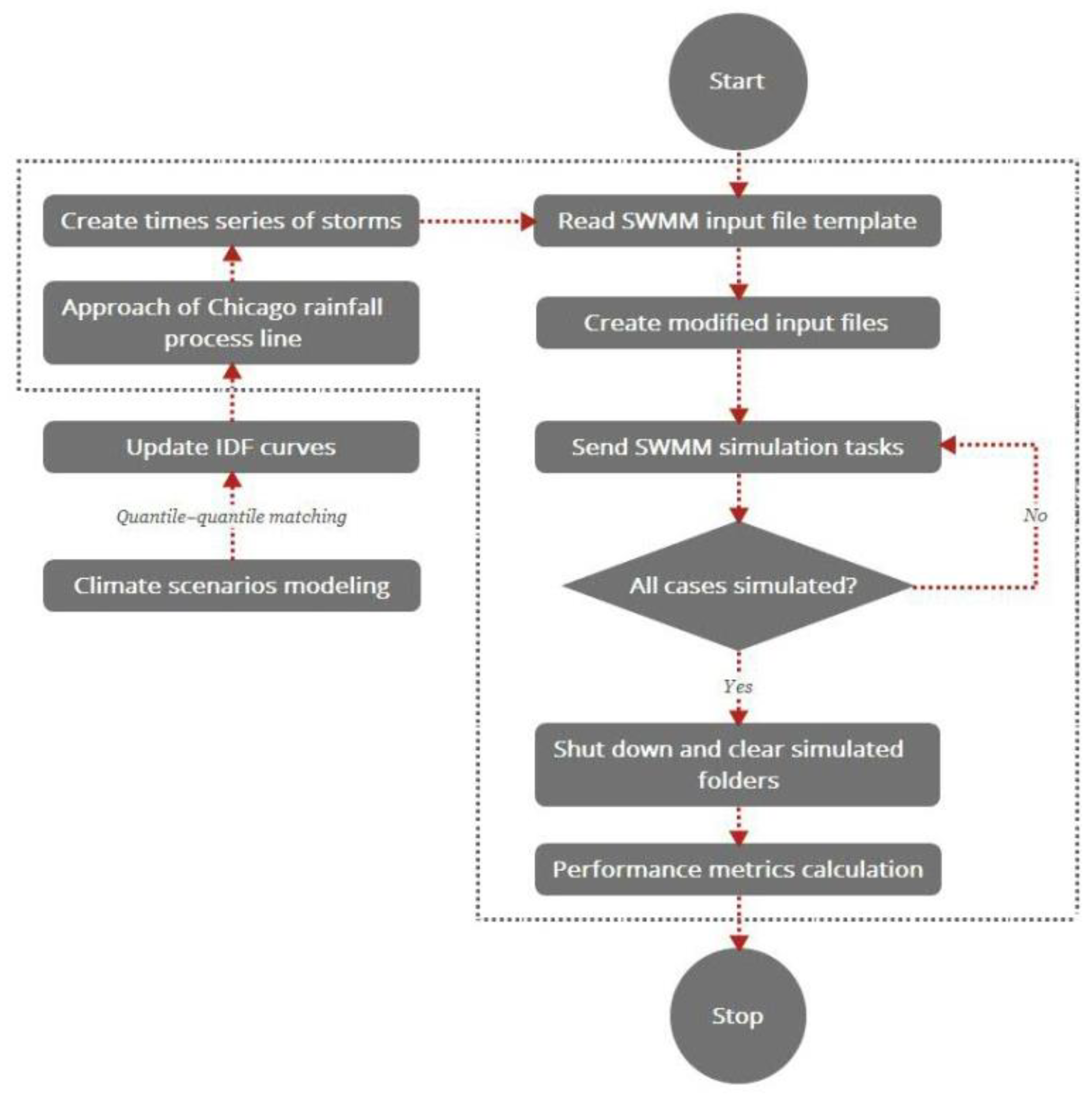
2.3. Hydrological Model

The Storm Water Management Model (SWMM), version 5.1 (Environmental Protection Agency, Washington, D.C., USA), was used to assess the hydro-performance of BCs in this study. SWMM has been widely used for analysis, planning, and design of various LID practices, including BCs in small urban catchments [46]. In SWMM, BCs are represented as structures including (from top to bottom) surface layer, filter layer, transition layer, and drainage layer, as well as outflow structures (Figure 1). Actually, vegetation also plays a critical role in the water balance of BCs by improving infiltration and facilitating evapotranspiration. There are various potential impacts on the hydrological performance of BCs because of different scales and species vegetated on the surface layer. However, there is only vegetation volume fraction as a parameter for simulating hydrological effects of BCs due to the limited information of vegetation for BCs in this study. The properties of the filter layer are sandy loam (50%) and medium to coarse sand (1–2 mm, D60 (Particle size of the filter with a cumulative weight of 60%) = 2 mm) (50%)) from top to bottom. The transition layer (50 mm) is comprised by coarse sand (0.5–2 mm; D60 = 1 mm). In SWMM, infiltration estimation is by the Green-Ampt method, percolation is modeled using Darcy’s law, and dynamic wave routing solves one-dimensional Saint Venant flow equations for flow routing [47]. The hydrologic cost-effectiveness of BCs can be simulated by water balance equations. Since the hypothetical catchment is simply imitating the representative characteristics of a dense urban surface, it still could effectively elucidate and project the uncertainty and influences of climate changes as the focus of the study without any calibration or verification of SWMM for BCs. The major parameters of the baseline scenario simulated by SWMM are shown in Table 2. After the completion of simulation, SWMM exports the summary statistics and time series into a report file (.rpt) and output files (.txt or .dat).
A toolbox based on the R programming language [48] was developed to automate the process, including modifying input files, extracting results, and calculating performance metrics, since SWMM is a console application that is very time-consuming when it handles a multitude of data inputs. As shown in Figure 2, the toolbox reads an input template according to scenario modeling and creates modified input files. Then the R process is used as the ‘master’ cluster node, which creates folders containing SWMM files, such as executable functions, input files, and rainfall time series [11]. Once the simulation is finished, the SWMM output files are moved to the designated folder and the master node is informed of job completion. The master node then determines whether all cases have been simulated; if so, it shuts down and clears the folders, and if not, it continues to assign new tasks. The SWMM output files of all cases are then read by the toolbox and used for performance metric calculations and further analysis.

2.4. Performance Metrics Calculation

2.4.1. Runoff Volume Reduction

The reduction of runoff volume based on event i ( R RV ( i ) ) is defined as the difference in runoff volume between event i and that for the baseline scenario (without BCs), and it is expressed as a percentage:
R RV ( i ) = ( V b V i ) V b × 100
where V b is the total inflow of the rainfall event in the baseline scenario, and V i is the bypass surface runoff volume discharged to O1 outlet of BCs on event i.
The summaries of total inflow and the bypass surface runoff from the SWMM report files in all scenarios were read in the R toolbox, and R RV ( i ) was calculated using Equation (4).

2.4.2. Peak Flow Reduction

The reduction of peak flow ( R PF ( i ) ) was calculated in the same way:
R PF ( i ) = ( P b P i ) P b × 100
where P b and P i are the peak runoff from rainfall in the baseline scenario and in event i, respectively.
The summaries of total peak runoff in all scenarios from the SWMM report files were read in the R toolbox, and R PF ( i ) was calculated using Equation (5).

2.4.3. First Flush Control

First flush control is usually relative, with the cumulative runoff depth reaching some threshold [49]. If the total inflow depth of a storm is smaller than this threshold, it can be viewed as the “initial portion”. The reduction of first flush ( R FF ( i ) ) was calculated using Equations (6) and (7).
R FF ( i ) = Q Initial storage ( D / D i * ) × 0 T i q i * ( t ) d t × 100 ,   if   D i * D
R FF ( i ) = 100 ,   if   D i * < D
where Q Initial storage is the initial storage volume of the BCs, D is the depth threshold (e.g., 10 mm, 20 mm, or 30 mm), D i * is the entire inflow depth of event i, 0 T i q i * ( t ) d t is the inflow volume of event i with different scales of BCs implemented, and t is the duration of event i.
The summaries of initial storage volumes, total precipitation, and inflow volumes from the SWMM report files were read in R the toolbox, and R FF ( i ) was calculated using Equations (6) and (7).

3. Results and Discussion

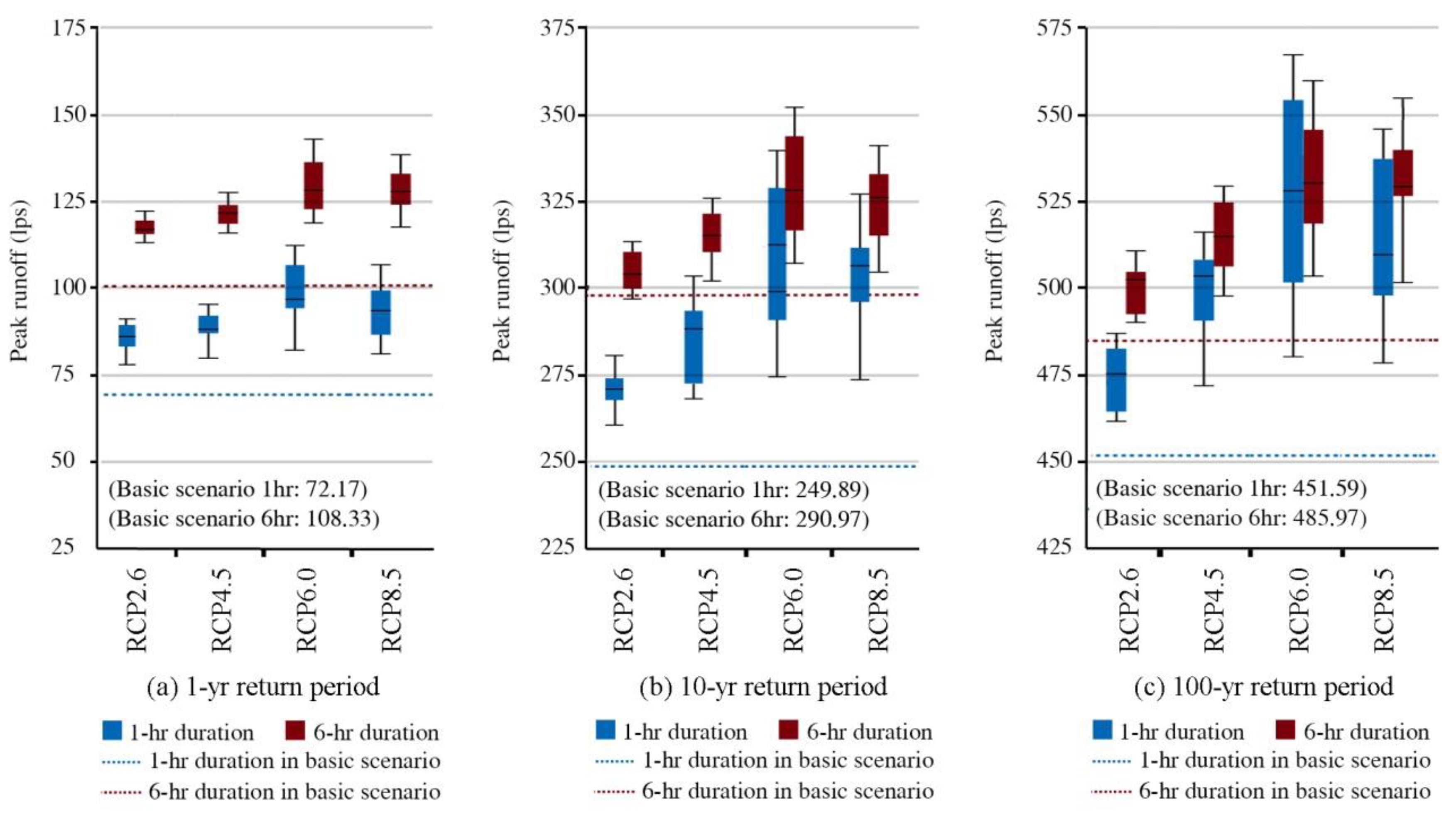
3.1. Effects of Climate Change on Storm Runoff

Climate change is intensifying the global hydrological cycle, notably making the peak flow increasingly strong in urban catchments, with increased frequency and severity of waterlogging, especially in dense urban areas with high imperviousness of surface [50]. The arithmetic mean of peak runoff for the test catchment in the baseline scenario and climate change scenarios is summarized in Table 3. The simulation showed similar trends across different climate scenarios. In almost all scenarios modeled, the events which showed dramatic variations had higher peak flows (Figure 3).
Peak flows become significantly larger in the climate change scenarios (Figure 3). Especially in RCP8.5, the median peak runoff percentage increases by 33.2%, 25.1%, and 16.9% for 1-, 10-, and 100-year storms with 1 h duration, due to dramatic challenges to adaptation and to mitigation of climate change by high emissions and low sustainability of development. The variations of peak flow in RCP2.6 were clearly smaller due to the relatively slight variations in climate (RCP2.6 is a relatively low-emissions scenario). The median peak flow rate increases by 9.9%, 4.5%, and 3.5% for the 1-, 10-, and 100-year storm events, with 6 h duration. Frequent rainfall events tend to be associated with bursts and are highly non-uniform both in space and time. Whereas heavy storms tend to be associated with wider spatial coverage and more voluminous rain clouds, and hence are more uniform in both space and time [51,52]. As might be expected, other scenarios showed increased intermediates between RCP2.6 and RCP8.5, since rainfall intensity increased moderately in these scenarios. Other work focusing on the projection of climate reported similar findings based on the ScenarioMIP experimental design [9,53].
For storms with different return periods, the changes (absolute value of Q3–Q1) of peak flow were higher for the 10-year and 100-year storms than for 1-year storms. This is consistent with other studies which found that climatic change may lead to more serious impacts particularly for storms with longer return periods, at least in the mid-latitudes [54]. However, comparing the ratios of changes, the variation of peak flow for longer return periods is smaller than for shorter return periods. For example, in RCP8.5 with 1-h events, the average increase in peak flow (31.7%) for the 1-year return period is larger than that for 10-year (20%) and 100-year (14%) events. Thus, uncertain future changes will lead to larger adverse influences on the quantity of runoff during relatively low-frequency rainfall events. Similar findings have been reported based on future scenario modeling [27,34]. Comparing 1-h and 6-h storms, the variations in peak flow in shorter storms are larger than those in longer ones, whether in absolute value or as a ratio compared to the baseline scenario. For example, in RCP8.5 with 10-year events, the average increase in peak flow in 1-h storms (20.0%) is larger than in 6-h storms (13.1%). In addition, the variation is nearly 65 L sec-1 in 1 h storms, compared to 46 L sec-1 in 6-h storms. Some other studies have found that the biggest increases are more likely in brief rainfall events, which implies a higher frequency and greater intensity of flash floods [40]. Dense urban catchments with a high percentage of impervious surfaces would be seriously challenged by such events. Therefore, to ensure effective management of surface runoff using LID, the scales of LID to be implemented should be assessed in response to the variations of storms caused by climate change, especially frequent and short-duration storms.

3.2. Performance of BCs in Climate Scenarios

3.2.1. Runoff Volume Reduction

The runoff volume reductions ( R RV ) in BCs with various scales were calculated using Equation (1), and the required scales of BC to meet specific levels of R RV were then derived. Generally, the scale of BCs should be increased as greater performance is needed (Table 4). Regression analysis of different return periods, durations, and scales of BCs can be studied as look-up curves in diverse scenarios. We selected RCP2.6 and RCP8.5 as representative pathways which reflected the minimum and maximum variations caused by climate change for comparative analysis.
R RV displays similar trends across various scenarios in the test catchment. R RV increases with the area of BCs, especially when the area is less than 5% of the test catchment (Figure 4a–c). The effectiveness of BCs in reducing runoff volume shows only slight changes across scenarios for 1 year storms (Figure 4d). With 8% area, for example, the simulated runoff reduction was 79.0%, 79.4%, and 70.3% for the baseline scenario, RCP2.6, and RCP8.5, respectively, for 1-year, 1-h storms. However, there is an obvious decrease in effectiveness under longer return period (e.g., 100 year) events (Figure 4e). For instance, the reduction with 10% area is only 34.1%, 21.5%, and 20.4% for the baseline scenario, RCP2.6, and RCP8.5, respectively. R RV is 35.9% with 20% of BCs coverage in RCP8.5 for a 100-year, 6-h storm. In contrast, there is complete control with 12% of BCs coverage in the baseline scenario for a 1-year, 1-h event. The difference may be due to the limited capacity of BCs to cope with large storms [55]. Moreover, the marginal improvement declined with greater coverage of BCs [10]. For 1-year, 6-h storms, going from 5% to 10% of surface area, BCs could produce an additional 30.5% reduction in RCP2.6; but going from 10% to 15% brought only another 20.3% reduction.
These results suggest that BCs may not be able to fully retain runoff volume, especially during larger storms. A trade-off in the amount of runoff retention has to be considered: larger BCs areas do help, but with diminishing marginal effectiveness.

3.2.2. Peak Flow Reductions

Several studies have found that the performance of BCs in reducing peak runoff to mitigate flood risk varies widely in different storms [56,57,58]. Peak runoff reductions ( R PF ) provided by various scales of BCs corresponding to different scenarios and design storms were calculated using Equation (2). Surface runoff from the catchment is collected by BCs, and during small storm events, all of the runoff can be retained in the ponding zone and do not overflow from the surface layer. Thus, effective reduction of peak flow is provided. However, retention volumes within BCs can be filled during large storms, and then there is very little reduction of runoff velocity in the bypass flows. Therefore, overflow occurrence timing and the shape of the inflow hydrograph can significantly change peak runoff [11].
The performance of BCs in the reduction of peak runoff can be observed in Table 5 for three scenarios: the baseline scenario, RCP2.6, and SSP3-8. The look-up curves were distinctly different in these scenarios (Figure 5): Larger scales of BCs were required to meet high reduction rates in storm events, while relatively small scales of BCs were required in small storms to achieve the same or better reduction rates. However, this finding is in contrast with some previous studies [11]. If relatively frequent storms with short duration were of interest, reduction exceeded 15% in all scenarios with 1-year, 1-h storms. However, they are very much ineffective for less frequent, heavier and longer duration storms. For instance, the reduction is less than 10% in RCP8.5 (the worst scenario), even with a large area.
This finding suggests that BCs could not replace conventional runoff management practices but should be integrated with them in the test catchment. The ability of BCs to control peak flow is limited for extreme storms (i.e., R PF is less than 20% in the baseline scenario). As the intensity of climate change increased, BCs were less and less help [18]. It was noted that the effects of vegetation planted on BCs for reducing the peak runoff are not considered in this study.

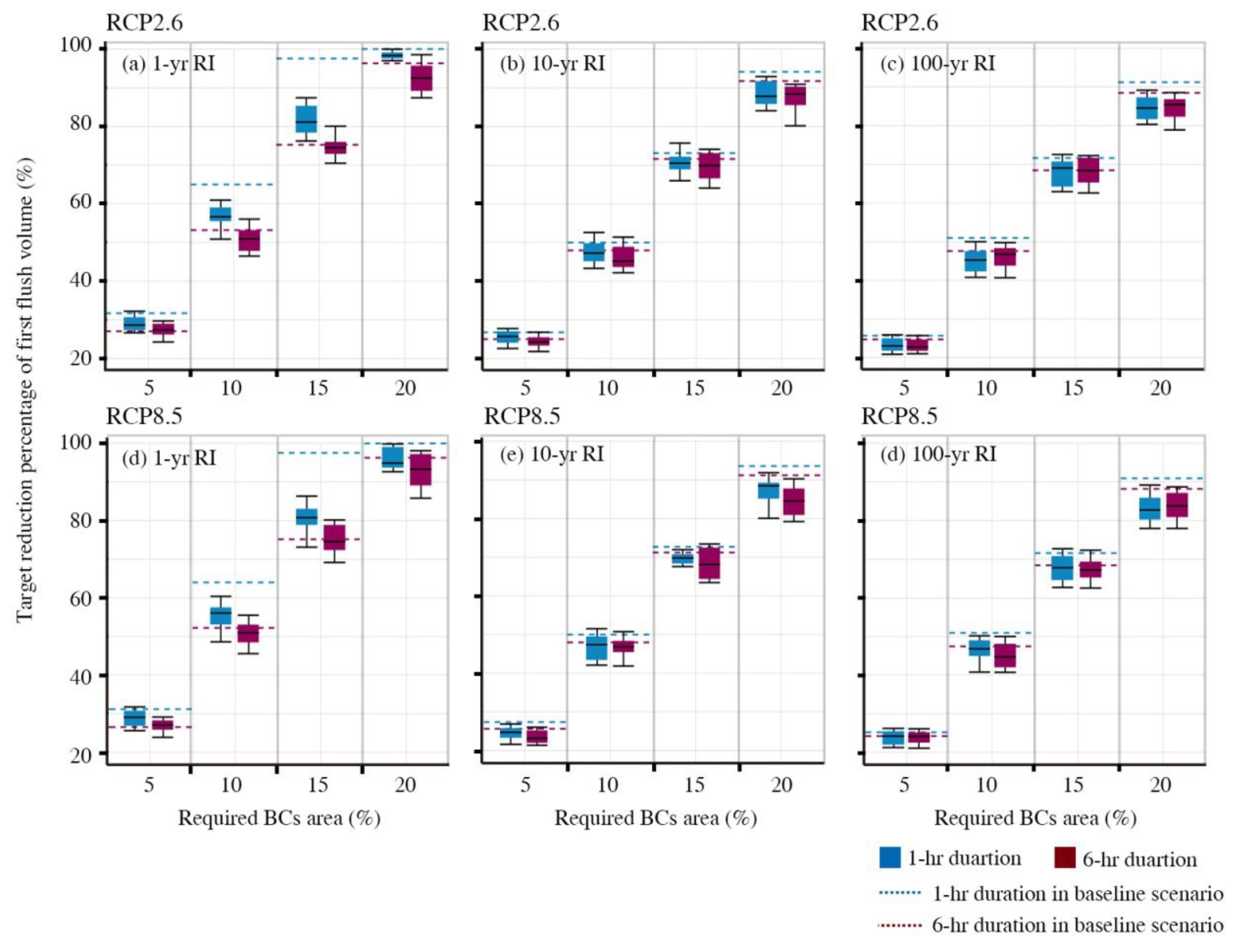
3.2.3. First Flush Control

First flush phenomena have been frequently reported in dense urban catchments [59]. Mitigating the initial portion of surface runoff may reduce non-point pollution of receiving water-bodies [60]. The first flush volume reductions ( R FF ) with different scales of BCs were computed using Equations (3) and (4). A depth threshold of 10 mm was used. Then, the required scales of BCs for performance targets of first flush control in each scenario were derived (Table 6). The required scales of BCs increased with a rising target R FF . With significant coverage, BCs were clearly effective in reducing first flush. At around 10% of the surface area, roughly half of the first 10 mm runoff was eliminated in all scenarios.
Figure 6 shows a set of required surface areas (5%, 10%, 15%, and 20%) of BCs for different R FF targets. Although there is some uncertainty, performance is slightly worse in the climate change scenarios than in the baseline scenario, due to the risk of flash runoff with the more intense storms caused by climate change. Moreover, performance declines as the return period of storms increases, and performance is better in brief events than in those of long duration, in all scenarios.
The initial storage volumes of BCs with the same parameters are the same. Therefore, for the same reduction performance, a greater area of BCs was needed for a higher depth threshold. This suggests that a suitable management objective must be selected: If objectives are set too high, then the required area will be very large, and BCs may not be able to fully eliminate the first flush, at least at a reasonable cost. To ensure the runoff quality of the receiving water-body, the rainfall depth threshold must be carefully designed according to the pollutant wash-off characteristics of the urban catchment.

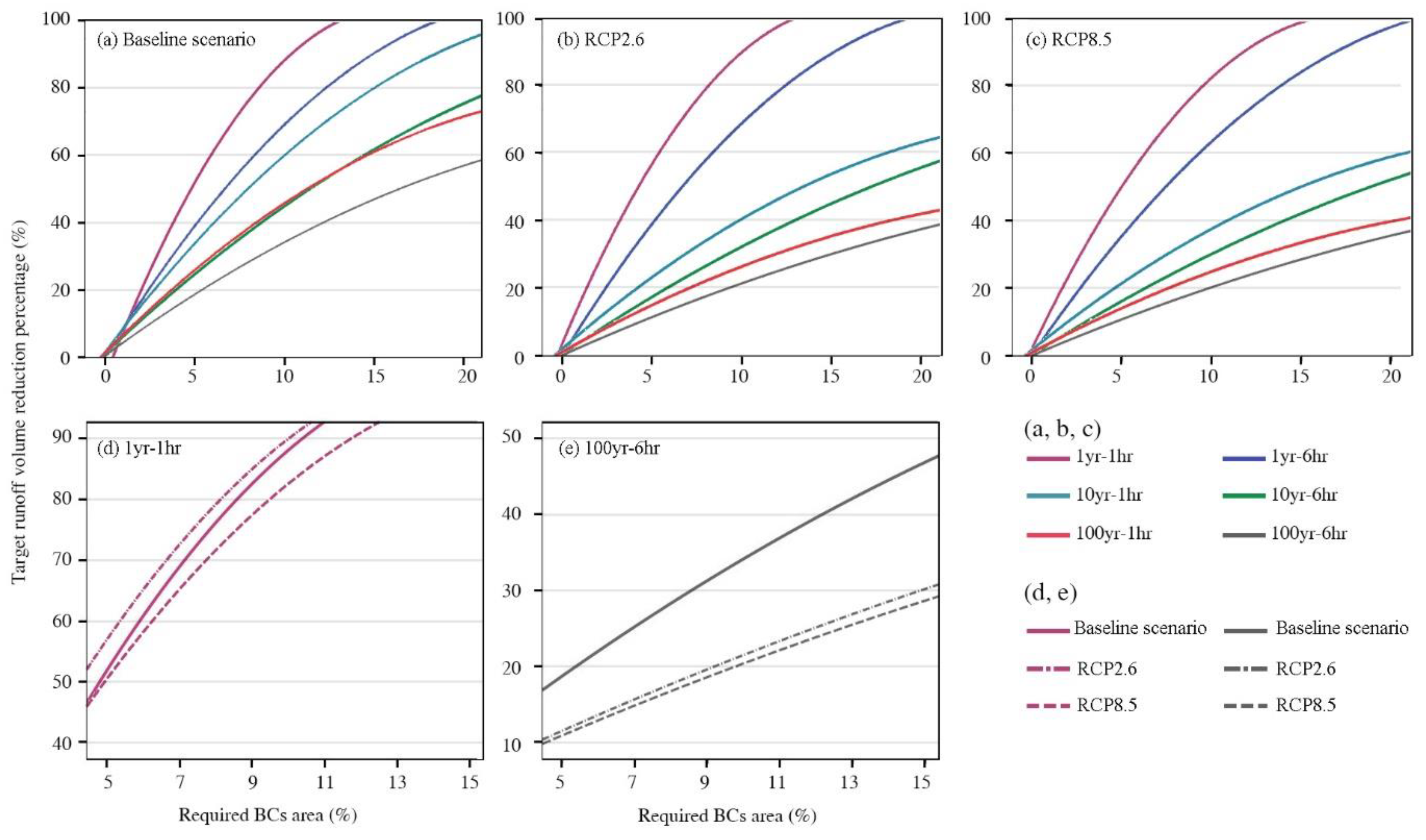
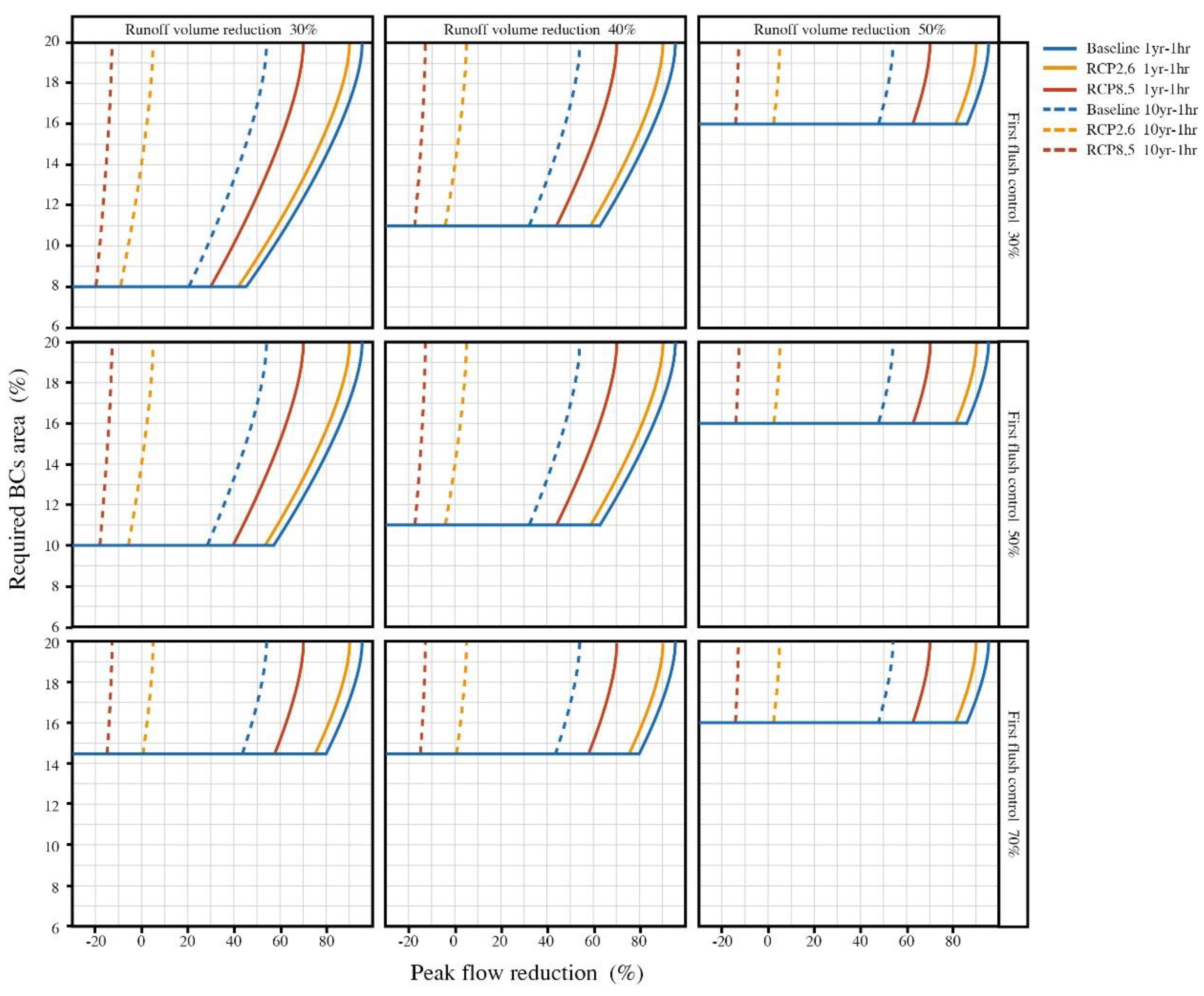
3.3. Targeted Scales of BCs in Response to Climate Change

BCs have the potential to be adopted widely in urban catchments. Before developing a master plan for LID to manage runoff, it is important to design optimal practices given the uncertainty of climate change and maximize the hydro-environmental benefits for limited resources and costs.
As mentioned, in view of the management interests of BCs regarding multiple objectives including runoff quantity and quality, developing multi-look-up curves for optimizing the cost-effectiveness of BCs in response to the challenges of climate change is critical. The multi-look-up curves for sizing can be generated by combining the single-objective look-up curves for Equations (4)–(7).
A set of look-up curves for selecting a rational scale of BCs to provide certain levels of R PF , while given requirements for R RV and R FF , are fulfilled in the baseline scenario, RCP2.6, and RCP8.5 with 1-year, 1-h and 10-year, 1-h design storms, are presented in Figure 7. The minimum area of BCs required increases with higher target R RV and R FF , regardless of the R PF target. In addition, the area of BCs required for the same level of reduction generally increases with storm intensity and the influence of climate change. For instance, to ensure at least 40% R RV and 50% R FF , 80% R PF is provided by 16% BCs in RCP2.6 with a 1-year, 1-h design storm, while 61% R PF is provided by the same BCs in RCP8.5.
The optimization results can help policymakers determine BC’s adoption with high-performance requirements and limited resources (e.g., space or budget) under potential influences of climate change. The R toolbox we developed can be used for the optimization of R PF , R RV , and R FF functions and to conduct case studies at other sites based on climate scenario modeling by adjusting the model parameters in SWMM. This simulation–optimization method could also be used to study other LID practices such as green roofs and infiltration trenches.

4. Conclusions

Climate scenario modeling for the influence of storm runoff was carried out to assess the performance of BCs in a high-density urban catchment. Storms with a short return period and short duration have more significant impacts than other storms. The influence is most adverse in RCP8.5, while it is relatively slight in RCP2.6. However, urban hydrology will unavoidably suffer from varying degrees of adverse effects in climate change scenarios compared to the present situation. Hence, more study is necessary to ensure the performance of BCs in a wide range of scenarios.
An optimized area for BCs to manage runoff can be determined based on a single objective (peak flow reduction, runoff volume reduction, or first flush control) or multiple objectives (i.e., a combination of the single objectives) in response to various potential climate changes using hydrology and climate scenario modeling. The case study of Guangzhou shows that BCs are relatively effective at managing the volume of inflow runoff and initial flow. However, as events increase in return period and duration, as well as the adverse influence of climate change, the effectiveness of BCs falls accordingly. In addition, the capacity of BCs to reduce the runoff volume and first flush of larger storms is limited, especially in climate change scenarios.
BCs are quite effective in controlling peak runoff in small storms of short duration. However, in larger storms, their performance is very limited, regardless of their implementation area, especially if we add the effects of climate change. Even large areas of BCs may not be able to replace conventional grey stormwater infrastructure. To maximize the system-wide hydro-environmental cost-effectiveness of BCs, optimizing the area of BCs intended to manage runoff during the more frequent rainfall events that will come with climate change should be the focus, given the reality of urban catchments with limited resources. In addition, the effects of plants in BCs should be further studied in the future.

Author Contributions

Conceptualization, M.W.; Data curation, M.W.; Investigation, Q.H., Y.L. and J.Q.; Methodology, M.W., D.Z. and S.K.T.; Project administration, Y.C.; Software, S.L.; Supervision, Y.C. and S.K.T.; Writing—original draft, M.W.

Funding

National Natural Science Foundation of China: 51808137; 51838003.

Conflicts of Interest

The authors declare no conflict of interest.

References

  1. Stott, P.A.; Christidis, N.; Otto, F.E.L.; Sun, Y.; Vanderlinden, J.; van Oldenborgh, G.J.; Vautard, R.; von Storch, H.; Walton, P.; Yiou, P.; et al. Attribution of extreme weather and climate-related events. WIREs Clim. Chang. 2016, 7, 23–41. [Google Scholar] [CrossRef] [PubMed]
  2. Wang, M.; Zhang, D.Q.; Adhityan, A.; Ng, W.J.; Dong, J.W.; Tan, S.K. Conventional and holistic urban stormwater management in coastal cities: A case study of the practice in Hong Kong and Singapore. Int. J. Water Resour. Dev. 2018, 34, 192–212. [Google Scholar] [CrossRef]
  3. Reshmidevi, T.V.; Kumar, D.N.; Mehrotra, R.; Sharma, A. Estimation of the climate change impact on a catchment water balance using an ensemble of GCMs. J. Hydrol. 2018, 556, 1192–1204. [Google Scholar] [CrossRef]
  4. Wang, L.; Chen, W. A CMIP5 multimodel projection of future temperature, precipitation, and climatological drought in china. Int. J. Climatol. 2014, 34, 2059–2078. [Google Scholar] [CrossRef]
  5. Moss, R.; Edmonds, J.; Hibbard, K.; Manning, M.; Rose, S.; van Vuuren, D.P.; Carter, T.; Emori, S.; Kainuma, M.; Kram, T.; et al. The next generation of scenarios for climate change research and assessment. Nature 2010, 463, 747–756. [Google Scholar] [CrossRef]
  6. Taylor, K.E.; Stouffer, R.J.; Meehl, G.A. An overview of CMIP5 and the experiment design. Bull. Am. Meteorol. Soc. 2012, 93, 485–498. [Google Scholar] [CrossRef]
  7. Fix, M.J.; Cooley, D.; Sain, S.R.; Tebaldi, C. A comparison of U.S. precipitation extremes under RCP8.5 and RCP4.5 with an application of pattern scaling. Clim. Chang. 2018, 146, 335–347. [Google Scholar] [CrossRef]
  8. Bacmeister, J.T.; Reed, K.A.; Hannay, C.; Lawrence, P.; Bates, S.; Truesdale, J.E.; Rosenbloom, N.; Levy, M. Projected changes in tropical cyclone activity under future warming scenarios using a high-resolution climate model. Clim. Chang. 2018, 146, 547–560. [Google Scholar] [CrossRef]
  9. O’Neill, B.C.; Tebaldi, C.; van Vuuren, D.P.; Eyring, V.; Friedlingstein, P.; Hurtt, G.; Knutti, R.; Kriegler, E.; Lamarque, J.-F.; Lowe, J.; et al. The scenario model intercomparison project (ScenarioMIP) for CMIP6. Geosci. Model Dev. 2016, 9, 3461–3482. [Google Scholar]
  10. Eckart, K.; Mcphee, Z.; Bolisetti, T. Multiobjective optimization of low impact development stormwater controls. J. Hydrol. 2018, 562, 564–576. [Google Scholar] [CrossRef]
  11. Yang, Y.; Chui, T.F.M. Optimizing surface and contributing areas of bioretention cells for stormwater runoff quality and quantity management. J. Environ. Manag. 2018, 206, 1090–1103. [Google Scholar] [CrossRef]
  12. Davis, A.P.; Hunt, W.F.; Traver, R.G.; Clar, M. Bioretention technology: Overview of current practice and future needs. J. Environ. Eng. 2009, 135, 109–117. [Google Scholar] [CrossRef]
  13. Davis, A.P. Field performance of bioretention: Hydrology impacts. J. Hydrol. Eng. 2008, 13, 90–95. [Google Scholar] [CrossRef]
  14. Wan, Z.X.; Li, T.; Liu, Y.T. Effective nitrogen removal during different periods of a field-scale bioretention system. Environ. Sci. Pollut. Res. 2018, 25, 17855–17861. [Google Scholar] [CrossRef]
  15. Wang, M.; Zhang, D.; Li, Y.; Hou, Q.; Yu, Y.; Qi, J.; Fu, W.; Dong, J.; Cheng, Y. Effect of a submerged zone and carbon source on nutrient and metal removal for stormwater by bioretention cells. Water 2018, 10, 1629. [Google Scholar] [CrossRef]
  16. Wang, M.; Zhang, D.; Dong, J.; Tan, S.K. Application of constructed wetlands for treating agricultural runoff and agro-industrial wastewater: A review. Hydrobiologia 2018, 805, 1–31. [Google Scholar] [CrossRef]
  17. Wang, M.; Zhang, D.Q.; Su, J.; Trzcinski, A.P.; Dong, J.W.; Tan, S.K. Future scenarios modeling of urban stormwater management response to impacts of climate change and urbanization. CLEAN—Soil Air Water 2017, 45, 1700111. [Google Scholar] [CrossRef]
  18. Chui, T.F.M.; Liu, X.; Zhan, W. Assessing cost-effectiveness of specific lid practice designs in response to large storm events. J. Hydrol. 2016, 533, 353–364. [Google Scholar] [CrossRef]
  19. Li, J.; Zhao, R.; Li, Y.; Chen, L. Modeling the effects of parameter optimization on three bioretention tanks using the hydrus-1D model. J. Environ. Manag. 2018, 217, 38–46. [Google Scholar] [CrossRef]
  20. Winston, R.J.; Dorsey, J.D.; Hunt, W.F. Quantifying volume reduction and peak flow mitigation for three bioretention cells in clay soils in northeast Ohio. Sci. Total Environ. 2016, 553, 83–95. [Google Scholar] [CrossRef]
  21. Baek, S.S.; Choi, D.H.; Jung, J.W.; Lee, H.J.; Lee, H.; Yoon, K.S.; Cho, K.H. Optimizing low impact development (LID) for stormwater runoff treatment in urban area, Korea: Experimental and modeling approach. Water Res. 2015, 86, 122–131. [Google Scholar] [CrossRef]
  22. Garcia-Cuerva, L.; Berglund, E.Z.; Rivers, L., III. An integrated approach to place green infrastructure strategies in marginalized communities and evaluate stormwater mitigation. J. Hydrol. 2018, 559, 648–660. [Google Scholar] [CrossRef]
  23. Hunt, W.F.; Smith, J.T.; Jadlocki, S.J.; Hathaway, J.M.; Eubanks, P.R. Pollutant removal and peak flow mitigation by a bioretention cell in urban Charlotte, NC. J. Environ. Eng. 2008, 134, 403–408. [Google Scholar] [CrossRef]
  24. Wang, M.; Zhang, D.Q.; Su, J.; Dong, J.W.; Tan, S.K. Assessing hydrological effects and performance of low impact development practices based on future scenarios modeling. J. Clean. Prod. 2018, 179, 12–23. [Google Scholar] [CrossRef]
  25. Hathaway, J.M.; Brown, R.A.; Fu, J.S.; Hunt, W.F. Bioretention function under climate change scenarios in North Carolina, USA. J. Hydrol. 2014, 519, 503–511. [Google Scholar] [CrossRef]
  26. Zahmatkesh, Z.; Karamouz, M.; Goharian, E.; Burian, S.J. Analysis of the effects of climate change on urban storm water runoff using statistically downscaled precipitation data and a change factor approach. J. Hydrol. Eng. 2014, 20, 05014022. [Google Scholar] [CrossRef]
  27. Borris, M.; Leonhardt, G.; Marsalek, J.; Österlund, H.; Viklander, M. Source-based modeling of urban stormwater quality response to the selected scenarios combining future changes in climate and socio-economic factors. Environ. Manag. 2016, 58, 223–237. [Google Scholar] [CrossRef]
  28. Wu, C.H.; Huang, G.R.; Wu, S.Y. Risk analysis of combinations of short duration rainstorm and tidal level in Guangzhou based on Copula function. J. Hydrol. Eng. 2014, 33, 33–41. [Google Scholar]
  29. Huang, H.; Chen, X.; Zhu, Z.; Xie, Y.; Liu, L.; Wang, X.; Wang, X.; Liu, K. The changing pattern of urban flooding in Guangzhou, China. Sci. Total Environ. 2018, 622–623, 394–401. [Google Scholar] [CrossRef]
  30. Zhao, Y.; Zou, X.; Cao, L.; Xu, X. Changes in precipitation extremes over the pearl river basin, southern China, during 1960–2012. Quat. Int. 2014, 333, 26–39. [Google Scholar] [CrossRef]
  31. Zhang, H.; Wu, C.; Chen, W.; Huang, G. Assessing the impact of climate change on the waterlogging risk in coastal cities: A case study of Guangzhou, South China. J. Hydrometeorol. 2017, 18, 1549–1562. [Google Scholar] [CrossRef]
  32. Li, Y.C.; Zhang, D.Q.; Wang, M. Performance evaluation of a full-scale constructed wetland for treating stormwater runoff. CLEAN—Soil Air Water 2017, 45, 1600740. [Google Scholar] [CrossRef]
  33. Liu, Y.; Engel, B.A.; Flanagan, D.C.; Gitau, M.W.; McMillan, S.K.; Chaubey, I.; Singh, S. Modeling framework for representing long-term effectiveness of best management practices in addressing hydrology and water quality problems: Framework development and demonstration using a bayesian method. J. Hydrol. 2018, 560, 530–545. [Google Scholar] [CrossRef]
  34. Wang, M.; Zhang, D.; Adhityan, A.; Ng, W.J.; Dong, J.; Tan, S.K. Assessing cost-effectiveness of bioretention on stormwater in response to climate change and urbanization for future scenarios. J. Hydrol. 2016, 543, 423–432. [Google Scholar] [CrossRef]
  35. Li, L.; Jensen, M.B. Green infrastructure for sustainable urban water management: Practices of five forerunner cities. Cities 2018, 74, 126–133. [Google Scholar] [CrossRef]
  36. Keifer, C.J.; Chu, H.H. Synthetic storm pattern for drainage design. J. Hydraul. Div. 1957, 83, 1–25. [Google Scholar]
  37. Jia, H.F.; Ma, H.T.; Sun, Z.X.; Yu, S.; Ding, Y.W.; Yun, L. A closed urban scenic river system using stormwater treated with lid-bmp technology in a revitalized historical district in China. Ecol. Eng. 2014, 71, 448–457. [Google Scholar] [CrossRef]
  38. Mei, C.; Liu, J.; Wang, H.; Yang, Z.; Ding, X.; Shao, W. Integrated assessments of green infrastructure for flood mitigation to support robust decision-making for sponge city construction in an urbanized watershed. Sci. Total Environ. 2018, 639, 1394–1407. [Google Scholar] [CrossRef]
  39. Vineyard, D.; Ingwersen, W.W.; Hawkins, T.R.; Xue, X.; Demeke, B.; Shuster, W. Comparing green and grey infrastructure using life cycle cost and environmental impact: A rain garden case study in Cincinnati, OH. J. Am. Water Resour. Assoc. 2015, 51, 1342–1360. [Google Scholar] [CrossRef]
  40. Westra, S.; Fowler, H.J.; Evans, J.P.; Alexander, L.V.; Berg, P.; Johnson, F.; Kendon, E.J.; Lenderink, G.; Roberts, N.M. Future changes to the intensity and frequency of short-duration extreme rainfall. Rev. Geophys. 2015, 52, 522–555. [Google Scholar] [CrossRef]
  41. Van Vuuren, D.P.; Kriegler, E.; O’Neill, B.C.; Ebi, K.L.; Riahi, K.; Carter, T.R.; Edmonds, J.; Hallegatte, S.; Kram, T.; Mathur, R.; et al. A new scenario framework for climate change research: Scenario matrix architecture. Clim. Chang. 2014, 122, 373–386. [Google Scholar] [CrossRef]
  42. Li, H.; Sheffield, J.; Wood, E.F. Bias correction of monthly precipitation and temperature fields from Intergovernmental Panel on Climate Change AR4 models using equidistant quantile matching. J. Geophys. Res. Atmos. 2010, 115, D10101. [Google Scholar] [CrossRef]
  43. Srivastav, R.K.; Schardong, A.; Simonovic, S.P. Equidistance quantile matching method for updating IDF curves under climate change. Water Resour. Manag. 2014, 28, 2539–2562. [Google Scholar] [CrossRef]
  44. Langousis, A.; Veneziano, D.; Furcolo, P.; Lepore, C. Multifractal rainfall extremes: Theoretical analysis and practical estimation. Chaos Solitons Fractals 2009, 39, 1182–1194. [Google Scholar] [CrossRef]
  45. Simonovic, S.P.; Schardong, A.; Sandink, D.; Srivastav, R. A web-based tool for the development of intensity duration frequency curves under changing climate. Environ. Model. Softw. 2016, 81, 136–153. [Google Scholar] [CrossRef]
  46. Rossman, L.A.; Huber, W. StormWater Management Model Reference Manual Volume III e Water Quality; EPA/600/R-16/093US; EPA Office of Research and Development: Washington, DC, USA, 2016.
  47. Rossman, L.A. Storm Water Management Model User’s Manual, Version 5.0; National Risk Management Research Laboratory, Office of Research and Development, US Environmental Protection Agency: Washington, DC, USA, 2010.
  48. R Core Team. R: A Language and Environment for Statistical Computing; R Foundation for Statistical Computing: Vienna, Austria, 2017. [Google Scholar]
  49. Wang, J.; Chua, L.H.C.; Shanahan, P. Evaluation of pollutant removal efficiency of a bioretention basin and implications for stormwater management in tropical cities. Environ. Sci. Water Res. Technol. 2016, 3, 78–91. [Google Scholar] [CrossRef]
  50. IPCC. Climate Change 2014: Mitigation of Climate Change. Contribution of Working Group III to the Fifth Assessment Report of the Intergovernmental Panel on Climate Change; Cambridge University Press: Cambridge, UK, 2014. [Google Scholar]
  51. Noor, M.; Ismail, T.; Chung, E.S.; Shahid, S.; Sung, J. Uncertainty in rainfall intensity duration frequency curves of peninsular Malaysia under changing climate scenarios. Water 2018, 10, 1750. [Google Scholar] [CrossRef]
  52. Uraba, M.B.; Gunawardhana, L.N.; Al-Rawas, G.A.; Baawain, M.S. A downscaling-disaggregation approach for developing IDF curves in arid regions. Environ. Monit. Assess. 2019, 191, 245. [Google Scholar] [CrossRef]
  53. Riahi, K.; van Vuuren, D.P.; Kriegler, E.; Edmonds, J.; O’Neill, B.C.; Fujimori, S.; Bauer, N.; Calvin, K.; Dellink, R.; Fricko, O.; et al. The shared socioeconomic pathways and their energy, land use, and greenhouse gas emissions implications: An overview. Glob. Environ. Chang. 2017, 42, 153–168. [Google Scholar] [CrossRef]
  54. Kim, E.S.; Choi, H.I. Assessment of vulnerability to extreme flash floods in design storms. Int. J. Environ. Res. Public Health 2011, 8, 2907–2922. [Google Scholar] [CrossRef]
  55. Ahiablame, L.M.; Engel, B.A.; Chaubey, I. Effectiveness of low impact development practices: Literature review and suggestions for future research. Water Air Soil Pollut. 2012, 223, 4253–4273. [Google Scholar] [CrossRef]
  56. Baek, S.S.; Ligaray, M.; Park, J.P.; Shin, H.S.; Kwon, Y.; Brascher, J.T.; Cho, K.H. Developing a hydrological simulation tool to design bioretention in a watershed. Environ. Model Softw. 2017. [Google Scholar] [CrossRef]
  57. Yang, Y.; Chui, T.F.M. Rapid assessment of hydrologic performance of low impact development practices under design storms. J. Am. Water Resour. Assoc. 2018, 54, 613–630. [Google Scholar] [CrossRef]
  58. Pyke, C.; Warren, M.P.; Johnson, T.; LaGro, J., Jr.; Scharfenberg, J.; Groth, P.; Freed, R.; Schroeer, W.; Main, E. Assessment of low impact development for managing stormwater with changing precipitation due to climate change. Landsc. Urban Plan. 2011, 103, 166–173. [Google Scholar] [CrossRef]
  59. Al, A.S.; Bonhomme, C.; Dubois, P.; Chebbo, G. Investigation of the wash-off process using an innovative portable rainfall simulator allowing continuous monitoring of flow and turbidity at the urban surface outlet. Sci. Total Environ. 2017, 609, 17–26. [Google Scholar] [CrossRef]
  60. Shen, Z.; Liu, J.; Aini, G.; Gong, Y. A comparative study of the grain-size distribution of surface dust and stormwater runoff quality on typical urban roads and roofs in Beijing, China. Environ. Sci. Pollut. Res. 2016, 23, 2693–2704. [Google Scholar] [CrossRef]
Figure 1. The framework of assessing hydrological effects of bioretention cells in climate scenarios. Notes: GCMs = General circulation models, RCMs = Regional circulation models, EQM = Equidistance quantile-matching, P = precipitation, R = runoff, O1 = outlet of surface bypass runoff, O2 = outlet of underdrain outflow.
Water 11 00997 g001
Figure 2. Workflow of the proposed R toolbox.
Water 11 00997 g002
Figure 3. Peak runoff (L sec-1) from the test catchment based on climate scenarios and baseline scenarios. Note: In these boxplots, the base denotes the first quartile (Q1, 25%), the line in the central part of the box indicates the median (50%), and the roof marks the 3rd quartile (Q3, 75%). Large variability of peak runoff is found by the upper and lower of the whiskers.
Water 11 00997 g003
Figure 4. Reduction percentages of runoff volume provided by bioretention cells implemented in different areas under different design storms in Baseline scenarios, RCP2.6, and RCP8.5.
Water 11 00997 g004
Figure 5. Reduction percentages of peak runoff provided by bioretention cells implemented in different areas under different design storms in Baseline scenarios, RCP2.6, and RCP8.5.
Water 11 00997 g005
Figure 6. Reduction percentages of first flush volume provided by bioretention cells implemented in different areas (5%, 10%, 15%, and 20% of catchment) under different design storms in Baseline scenarios, RCP2.6, and RCP8.5.
Water 11 00997 g006
Figure 7. Required scales of bioretention cells implemented for multi-hydrological interests (x axis: peak flow reduction; subplots (horizontal labels): runoff volume reduction; subplots (vertical labels): first flush control) under 1yr–1hr and 10yr–1hr design storms in Baseline scenarios, RCP2.6, and RCP8.5. Depth threshold of the initial portion of runoff is 10 mm.
Water 11 00997 g007
Table 1. Parameters of test urban catchment (0.5 ha) and bioretention cells (BCs) in Storm Water Management Model (SWMM).
ParametersValues
CatchmentArea (m2)5000
Impervious rate (%)50
Slope (%)0.5
Depth of depression storage on pervious area (mm)20
BCs appliedArea of BCs applied in the catchment (%)0 to 20
Surface of BCsBerm height (mm)152
Vegetation volume fraction (m3/m3)0.05
Surface roughness (Manning’s n)0
Surface slope (%)0
Soil of BCsThickness of soil (mm)610
Porosity (m3/m3)0.52
Field capacity (m3/m3)0.15
Wilting point (m3/m3)0.08
Conductivity (mm/hr)119
Conductivity slope39.3
Suction head (mm)48
Storage of BCsThickness of storage (mm)305
Void ratio (voids/solids)0.67
Seepage rate (mm/hr)13
Clogging factor0
Underdrain of BCsFlow coefficient of drain2.5
Flow exponent of drain0.5
Offset height of drain (mm)152
Notes: Parameters of surface, soil, storage, and drain are from [18,39,40].
Table 2. Changes of rainfall intensities (%) for four RCPs compared for baseline in Guangzhou.
Guangzhou (N = 10)Duration (h)MinimumAverageMaximum
1-yr10-yr100-yr1-yr10-yr100-yr1-yr10-yr100-yr
RCP2.61.01.81.31.14.94.23.39.26.95.4
6.01.61.21.03.92.92.37.55.94.6
RCP4.51.04.23.42.811.49.27.117.113.110.3
6.03.52.72.37.46.15.312.69.57.8
RCP6.01.05.54.83.914.811.18.723.919.415.3
6.04.63.43.010.89.07.318.413.812.1
RCP8.51.06.35.24.216.912.19.427.922.718.8
6.05.34.13.312.910.58.221.516.913.5
Notes: source of information published by the China Meteorological Data Service Center, and Guangzhou Meteorology, and climate change knowledge portal of the World Bank Group for Guangzhou, China and [24,43].
Table 3. Peak runoff (L sec-1) simulated in baseline and climate scenarios in different design storms.
Scenarios1yr-1hr10yr-1hr100yr-1hr1yr-6hr10yr-6hr100yr-6hr
Baseline72250452108291486
RCP2.679271480115303502
RCP4.588289502120314520
RCP6.089296511125324531
RCP8.595300515128329536
Table 4. Reduction rates of runoff volume (%) simulated in baseline scenarios, RCP2.6, and RCP8.5.
ScenarioBaselineRCP2.6RCP8.5
Duration1 h6 h1 h6 h1 h6 h
Return Period1yr10yr100yr1yr10yr100yr1yr10yr100yr1yr10yr100yr1yr10yr100yr1yr10yr100yr
Required BCs area (%)113.210.27.39.15.94.316.46.54.19.03.92.514.36.03.98.23.62.4
216.210.313.117.211.28.328.611.67.417.17.64.925.110.77.015.77.14.7
318.225.213.625.016.112.139.316.110.324.711.17.234.514.99.722.710.46.8
439.225.222.832.020.815.648.820.313.031.914.59.543.118.812.229.313.59.0
549.337.727.238.725.219.157.224.215.538.717.811.650.622.414.635.616.611.0
658.137.731.445.329.722.265.027.917.945.320.913.757.625.816.941.619.513.0
774.348.235.351.633.825.472.231.220.251.723.915.864.129.019.147.522.314.9
879.453.038.957.837.528.179.034.422.457.826.817.770.332.021.253.125.016.8
981.757.542.462.441.131.385.237.524.563.729.619.776.034.823.158.627.718.6
1095.457.645.768.144.934.191.040.426.469.332.321.581.437.525.063.930.220.4
1195.565.948.973.448.237.096.443.228.374.335.023.386.540.226.868.832.822.1
12100.069.951.978.451.439.7100.045.930.178.437.625.191.342.728.573.435.223.8
13100.070.154.883.254.842.1100.048.531.982.340.126.895.745.130.177.137.625.4
14100.070.357.687.558.244.3100.051.033.686.042.628.599.947.431.880.639.927.0
15100.080.760.491.261.146.5100.053.435.289.545.030.1100.049.733.383.942.128.6
16100.081.062.994.764.348.9100.055.736.892.847.331.7100.051.934.887.144.330.1
17100.087.365.498.167.451.2100.058.038.395.949.633.3100.054.036.390.146.531.6
18100.087.667.9100.070.453.2100.060.239.898.451.934.8100.056.137.793.048.633.1
19100.093.270.2100.073.455.4100.062.341.3100.054.036.3100.058.139.195.750.634.5
20100.096.072.6100.076.157.2100.064.342.7100.056.237.8100.060.040.597.952.635.9
Table 5. Reduction rates of peak runoff (%) simulated in baseline scenarios, RCP2.6, and RCP8.5.
ScenarioBaselineRCP2.6RCP8.5
Duration1 h6 h1 h6 h1 h6 h
Return Period1 yr10 yr100 yr1 yr10 yr100 yr1 yr10 yr100 yr1 yr10 yr100 yr1 yr10 yr100 yr1 yr10 yr100 yr
Required BCs area (%)0000000−9.2−11.6−13.8−5.7−10.8−17.6−31.7−20.0−23.4−18.0−22.3−25.9
13.11.10.90.90.10.1−6.3−9.4−13.4−5.4−10.2−16.7−29.0−19.1−22.9−17.8−22.2−25.0
26.52.51.82.10.20.1−2.9−8.3−13.1−4.7−10.2−15.9−25.8−18.1−22.5−17.2−21.7−24.1
36.53.43.73.41.70.20.8−7.1−12.7−4.3−9.8−15.0−22.5−18.1−22.0−16.8−21.3−23.4
413.64.64.14.92.41.14.7−7.0−12.3−1.8−8.7−14.2−18.9−18.0−21.6−14.5−21.1−22.6
514.15.84.76.13.21.98.9−5.8−11.9−0.5−7.6−13.8−15.2−18.0−21.2−13.4−20.7−21.8
635.87.85.77.33.92.414.9−5.6−11.60.8−7.5−13.2−10.3−17.9−20.7−12.4−19.5−21.2
736.611.26.78.55.12.923.8−5.4−11.22.1−6.2−12.6−4.9−16.8−20.3−11.3−18.4−20.5
851.413.07.710.35.83.531.6−4.2−10.83.5−6.2−11.93.3−16.7−19.8−10.1−17.9−19.7
952.314.78.712.36.54.041.4−3.9−10.46.3−6.0−11.312.2−16.5−19.3−9.0−16.3−19.0
1079.115.09.713.97.24.552.9−3.6−10.09.9−5.6−10.624.1−15.4−18.9−7.1−15.7−18.3
1184.118.310.715.67.95.066.5−3.4−9.717.1−5.1−9.933.2−14.2−18.4−1.3−14.0−17.5
1295.820.111.817.28.75.694.7−2.1−9.325.2−4.6−9.246.7−13.0−17.93.5−13.4−16.7
1395.924.612.418.99.46.695.9−1.8−8.930.4−4.0−8.558.9−12.9−17.58.7−11.1−16.0
14100.029.412.839.710.17.197.8−1.4−8.441.8−3.8−7.893.6−11.7−17.018.0−10.6−15.2
15100.035.713.459.910.87.6100.0−1.1−8.049.7−3.4−7.194.7−10.5−16.527.5−10.0−14.4
16100.046.213.866.711.87.9100.0−0.5−7.659.7−3.0−6.496.2−9.2−16.033.1−9.4−13.6
17100.054.317.083.512.98.1100.00.0−7.270.7−2.6−5.698.6−8.0−15.545.3−8.9−12.8
18100.059.718.185.414.18.6100.00.1−6.981.5−1.1−4.9100.0−7.7−15.053.5−7.3−12.5
19100.063.819.286.015.58.6100.02.6−6.582.2−0.6−4.4100.0−6.3−14.566.1−6.7−11.4
20100.080.020.386.516.19.1100.05.7−6.283.02.1−3.4100.0−5.0−14.178.7−5.1−10.4
Table 6. Reduction rates of first flush control (%) simulated in baseline scenarios, RCP2.6, and RCP8.5 with the threshold of 10 mm.
ScenarioBaselineRCP2.6RCP8.5
Duration1 h6 h1 h6 h1 h6 h
Return Period1yr10yr100yr1yr10yr100yr1yr10yr100yr1yr10yr100yr1yr10yr100yr1yr10yr100yr
Required BCs area (%)0000.00.00.00.00.00.00.00000000000
16.75.85.56.05.65.46.55.55.25.95.35.26.35.45.25.85.35.2
213.35.810.911.811.010.612.810.810.311.710.610.312.410.710.311.510.510.2
320.017.110.817.516.315.819.016.015.417.315.715.318.315.915.317.015.615.2
426.716.921.423.121.520.825.021.220.322.820.720.124.221.020.222.520.620.1
533.327.826.428.526.625.830.826.225.128.225.624.929.825.924.927.825.524.8
640.027.631.433.831.630.636.531.129.833.430.429.635.330.829.632.930.229.5
746.638.136.239.036.535.342.135.834.438.535.134.240.735.534.238.034.934.1
853.343.141.044.141.240.047.540.538.943.539.738.746.040.238.742.939.538.5
960.047.945.649.045.944.552.845.143.348.444.243.151.244.843.147.844.042.9
1066.647.550.253.950.548.957.949.647.753.248.747.456.249.247.552.548.447.2
1173.357.354.658.655.053.363.054.151.957.953.051.661.153.651.757.252.751.5
1279.961.959.063.259.457.667.958.456.162.557.255.865.957.955.961.757.055.6
1386.661.363.367.863.761.872.762.660.267.061.459.870.662.160.066.161.159.7
1493.360.967.572.267.965.977.466.864.271.465.563.875.266.364.070.565.263.7
1599.974.971.676.672.069.982.070.968.275.769.567.879.770.367.974.869.267.6
16100.074.475.680.876.173.986.574.972.079.973.471.684.174.371.879.073.171.4
17100.083.279.685.080.077.790.978.875.884.177.375.488.478.275.583.077.075.2
18100.082.683.489.183.981.595.382.679.688.181.179.192.682.079.387.080.778.9
19100.091.287.393.187.885.399.586.483.292.184.882.896.785.882.991.084.482.6
20100.095.191.097.091.588.9100.090.186.896.088.586.4100.089.486.594.888.186.2

