Experimental Investigation of Purging Saline Solution from a Dead-End Water Pipe


1
Al Imam Mohammad Ibn Saud Islamic University, IMSIU, Riyadh 11432, Saudi Arabia
2
Irrigation and Hydraulics Department, Faculty of Engineering, Cairo University, Giza 12613, Egypt
3
Irrigation and Hydraulics Department, Faculty of Engineering, Ain Shams University, Cairo 11517, Egypt
*
Author to whom correspondence should be addressed.
Water 2019, 11(5), 994; https://doi.org/10.3390/w11050994
Submission received: 21 January 2019
/
Revised: 7 May 2019
/
Accepted: 8 May 2019
/
Published: 12 May 2019
(This article belongs to the Section Water Quality and Contamination)
Abstract
:Salty groundwater might find its way into dead end legs of a water distribution network and thus efforts are required to clean such parts of the network. This paper reports, for the first time, the results of a visual study for laboratory experimental investigation on the purging process of saline water from a dead-end water pipe using fresh water. Three purging locations and a number of purging flow rates were considered to identify the effect of purging location and purging flow rate on the time required to completely remove saline water from the dead-end pipe. Image processing analysis techniques were used to capture data from the experimental lab setup. A universal gray-intensity to salinity curve was experimentally found to formulate a color intensity to salinity mapping. A script code based on Octave numerical package was written for this regard to determine the temporal variation of the total dissolved salt (TDS) value within the dead leg pipe. It is generally noted that, as Reynolds number gets higher, the time removal ratio (t/ts) gets bigger. It is also noted that, as a purging location gets farther from the dead end, the time required for the complete removal of TDS increases exponentially.
1. Introduction
Dead ends in water distribution networks are well known for holding poor water quality characteristics in terms of high residence times, absence of residual disinfectants, and favorable corrosion conditions [1]. Since water in dead end legs is uncirculated, its quality might get deteriorated quickly posing high risk to health [2]. Studies of water distribution systems have repeatedly shown that bacteriological hot spots are three to four times more likely to occur at dead end areas in a distribution system [3]. For this regard, water operators and municipalities generally conduct periodic water flushing programs for the water network to clean the interior of the pipelines, to maintain disinfection residual, and to ensure the removal of sediment and biofilms from dead-end lines.
Different flushing techniques are commonly practiced including the conventional water flushing, Uni-Directional Flushing (UDF) and Impulsive Flushing methods. During the conventional flushing process, the flushing point (commonly the fire hydrant) at the targeted area is opened and water is moved freely from all directions until the water runs clear [4,5,6].
Despite of the common use of water Flushing techniques to improve water quality in the dead-ends of a network, in 2005, Barbeau et al. launched an on-site short and long-term monitoring program to monitor the status of water quality in two dead-end pipe locations after carrying out pipe flushing. Researchers noted that only minor improvement in the water quality took place after two weeks from conducting the pipe flushing [7]. Their findings suggest that more research efforts are still required.
The dead-end legs are generally located at the periphery of a distribution network; therefore, its pressure might score the minimum in the network and this might increase the risk of its vulnerability to get contaminated from nearby external sources. Such risks increase significantly in case of having an intermittent water distribution network as in most of the developing countries or in cities facing high water stress [8].
In case of intermittent network, water is generally supplied for short time periods (from 2 to 10 h per day) for a typical secondary city [9], therefore dead legs could be subjected to vacuum conditions after supply hours, which can allow saline groundwater to get into the water distribution network.
Purging a pipe is a terminology that is commonly used in natural gas and petroleum industry. For natural gas pipe network, purging means to clean a gas conduit of air or gas or to displace a hazardous or explosive gas by inert gas [10]. The goal of this study is to apply a simple and robust digital images-based colorimetry analytical method previously proposed by other researchers in other fields such as Reference [11] to assess the purging process of saline solution in a transparent dead leg pipe.
The study in hand is useful for the operation and maintenance of water distribution systems that have the following conditions:
- -
- The network includes dead end pipes;
- -
- The pipe network is subjected to quite long periods of low pressure. One might think that this problem exists only in intermittent pipe network, but recent lab research [12] proved that continuous-supply pipe network with pipe leaking point might be vulnerable to external contamination ingress too.
- -
- Existence of salt/contaminated groundwater in the vicinity of the water network and this salty/contaminated groundwater might get intruded inside the pipe system during the low-pressure periods;
- -
- Inaccessibility of the dead-end point and thus purging should be conducted from other point.
2. Methodology
Visual studies have transferred to a new era with the development and improvement of high speed and high-resolution cameras. Nowadays, image processing is widely used to capture time-dependent process data for many engineering applications. For instance, in soil and groundwater contamination, Reference [13] conducted image processing analysis to quantify the amount of trinitrotoluene in the water soil. In surface hydrology, [11] applied digital image-based colorimetry to determine the amount of Chromium and Iron in rivers and open channels. In hydropower, Reference [14] used freeware video analysis package (Tracker) to identify the instantaneous angular speed of a rotor fixed downstream of a sluice gate.
In this study, image processing and video analysis were conducted using the open source GNU Octave package, [15]. Script code was written to automate the steps of imaging process and to obtain the variation of the saline purging with the time course.
2.1. Preparation of Saline Solution
The study in-hand uses tap water as a purging liquid whereas saline solution is used to represent the liquid to be purged from the pipe dead leg. Three saline solutions of different salinities (1867, 9600, and 14,420 ppm) were initially used to determine the color-to-salinity conversion curve that will determine the relation between the gray intensity ratio and the salinity ratio.
In order to prepare a stock solution for each salinity, a 180 L-barrel was filled with tap water of initial TDS of 300 ppm. An amount of Sodium Chloride was added to water to reach the targeted maximum salinity. The salinity and temperature of the produced solution was measured using a TDS meter. Furthermore, five bottles of dark blue ink (30 mL each) were added to the stock solution for imaging purposes. The solution was then mechanically mixed for a couple of minutes to ensure solution homogeneity.
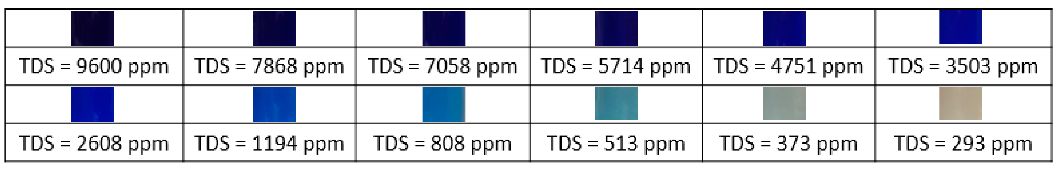
A sample of 400 mL of the stock solution was taken to prepare the Saline Solution Standard (SSS) that will be used for color calibration. The sample was further diluted with water several times to produce a matrix of saline solution samples with different TDS and color values. The resultant colors of SSS were photographed half a minute after color development using Sony RX100 camera. Figure 1 shows an example of the RGB (red–green–blue) color matrix of the prepared SSS as a function of the TDS values after successive dilution process for the solution of initial salinity of 9600 ppm.
The abovementioned steps were repeated to produce two other stock solutions of maximum salinities, 1867 and 14,420 ppm, respectively. The corresponding color matrices (similar to the one shown in Figure 1) for each stock solution were obtained.
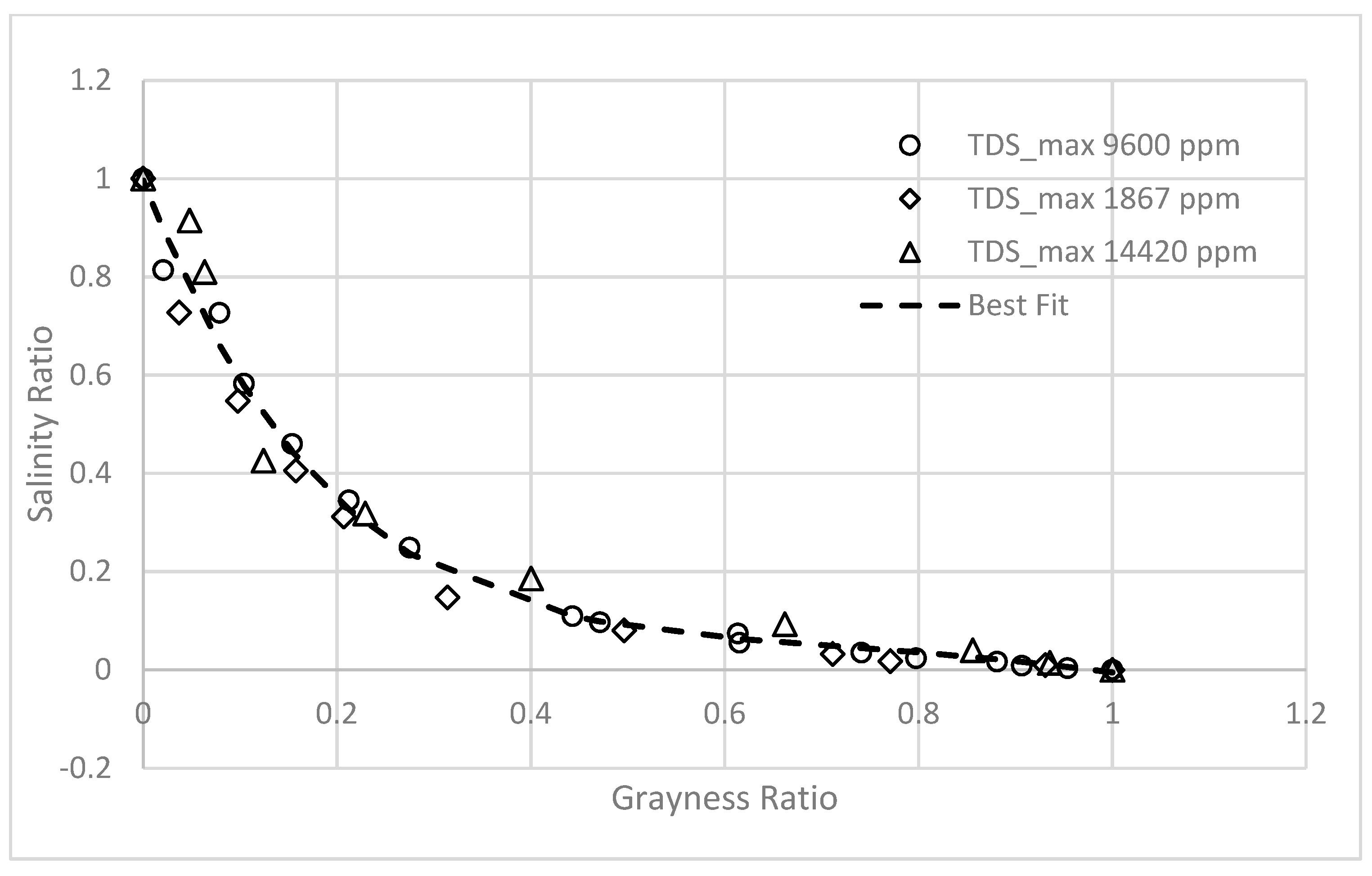
The produced color matrices were used to construct the color-to-salinity conversion curve that relates the color intensity value with the measured solute concentration. In order to do so, the RGB color image matrices were converted first to gray scale with gray intensity varying from 0 to 255. The gray intensity data were calculated from the averaging of the gray intensity values for at least 16 randomly selected points within the square-homogenous cropped images using Octave open source software.
Figure 2 shows the resulted data from the image processing of the color matrices for the three solutions (1867, 9600, and 14,420 ppm). The data are transformed in a normalized way such that the horizontal axis represents a dimensionless parameter called grayness ratio (Gr), whereas the vertical axis represents another dimensionless parameter called the salinity ratio. The grayness ratio is defined as:
where Grayi is the actual average gray intensity value of the current solute sample at a specified moment i;
Grayness ratio (Gr) = |Grayi − Grayo|/|Graym − Grayo|
Grayo is the average gray intensity value of the original tap water before adding salt to it (typically 300 ppm in this experiment);
Graym is the maximum gray intensity of the solute that corresponds to the maximum TDS value (before dilution);
The salinity ratio (Sr) is defined as:
where TDSi is the actual salt (TDS) value of the solute sample at a specified moment i;
Salinity ratio (Sr) = |TDSi − TDSo|/|TDSm − TDSo|
TDSo is the average TDS value of original water before adding salt to it (TDSo = 300 ppm);
TDSm is maximum TDS value of the solute (before dilution) (TDSm = 1867, 9600, and 14,420 ppm for the three solutions);
It is noted that a single universal color-to-salinity conversion curve (shown as dashed curve in Figure 2) can best fit all data that belong to different solutions of different salinities and the data can be represented mathematically as per the following decay exponential equation:
where a, b, c, and d are universal constants and their values are given in Table 1 below:
Gr = Max(0, a * Sr * exp(−b * Sr) + c * Sr + d)
The use of the maximum function in Equation (3) is not a mandatory however it is added in the equation to ensure the non-negativity of the salinity ratio that might be numerically encountered in case of having high values of grayness ration when numerical truncation of some of the digits of the universal constants (that are given in Table 1) took place.
2.2. Experimental Setup
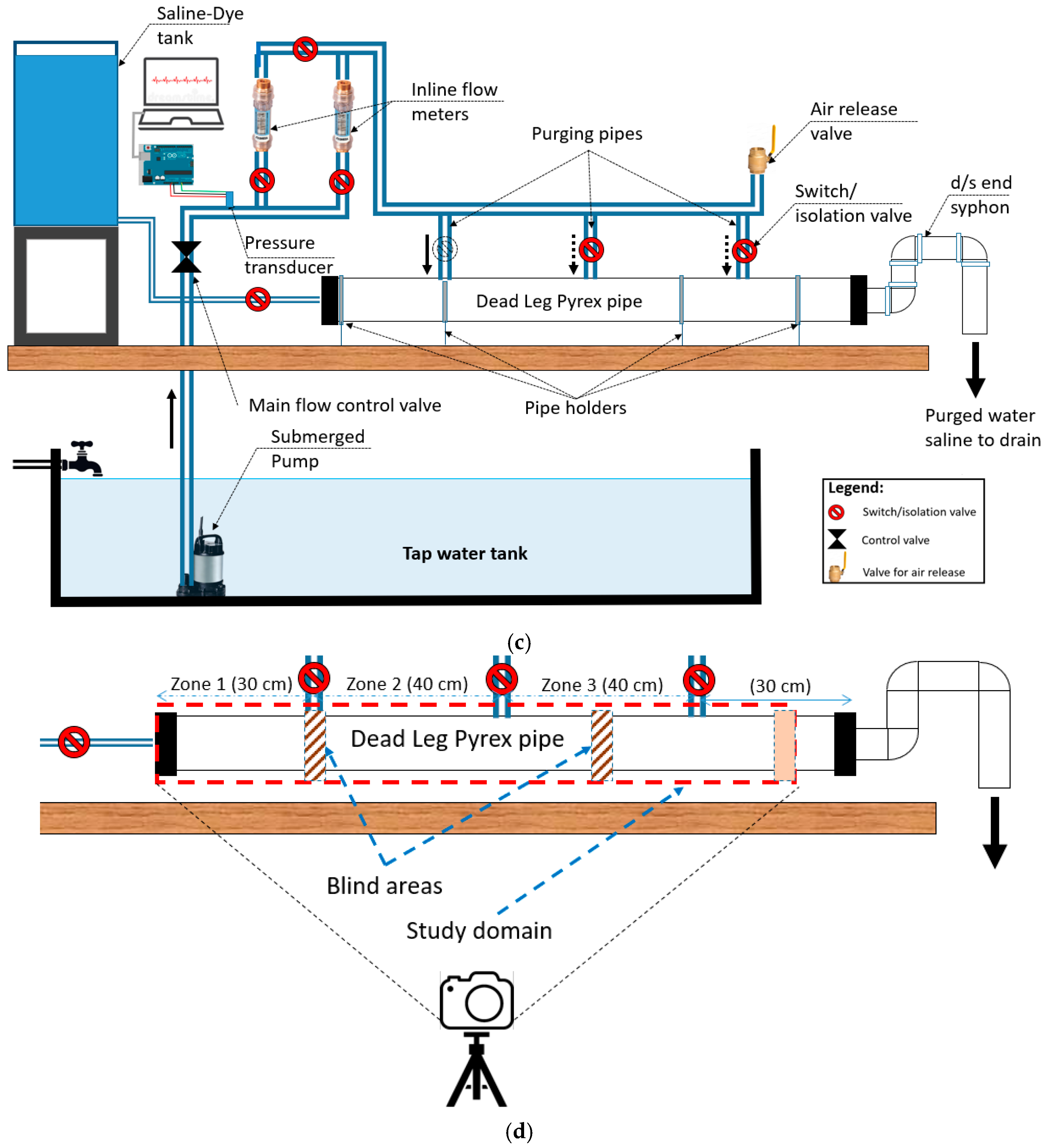
Figure 3 shows the experimental setup of the lab experiment that was used to investigate the purging process for a dead leg pipe. The system consists of a 4 inch (100 mm) in diameter dead leg pipe of length 140 cm. The pipe is made of Pyrex to allow for imaging of the internal solute motion. The first end of the dead leg pipe is connected to a 180-L stock solution tank (saline-dye tank) via a 1/2-inch (12.5 mm) flexible pipe with control valve, the downstream end of the dead leg pipe is connected to an inverted syphon, which freely drains to a final disposal drain.
The downstream end syphon is used to facilitate the process of complete refilling the pipe (at the start of each run) with saline water by retaining the dense saline water upstream of the syphon and preventing it from drainage downstream.
Three purging pipes (1.0 inch (25 mm) each in diameter and supplied with switch valves) are connected perpendicularly to the dead leg pipe to study the purging process at different locations.
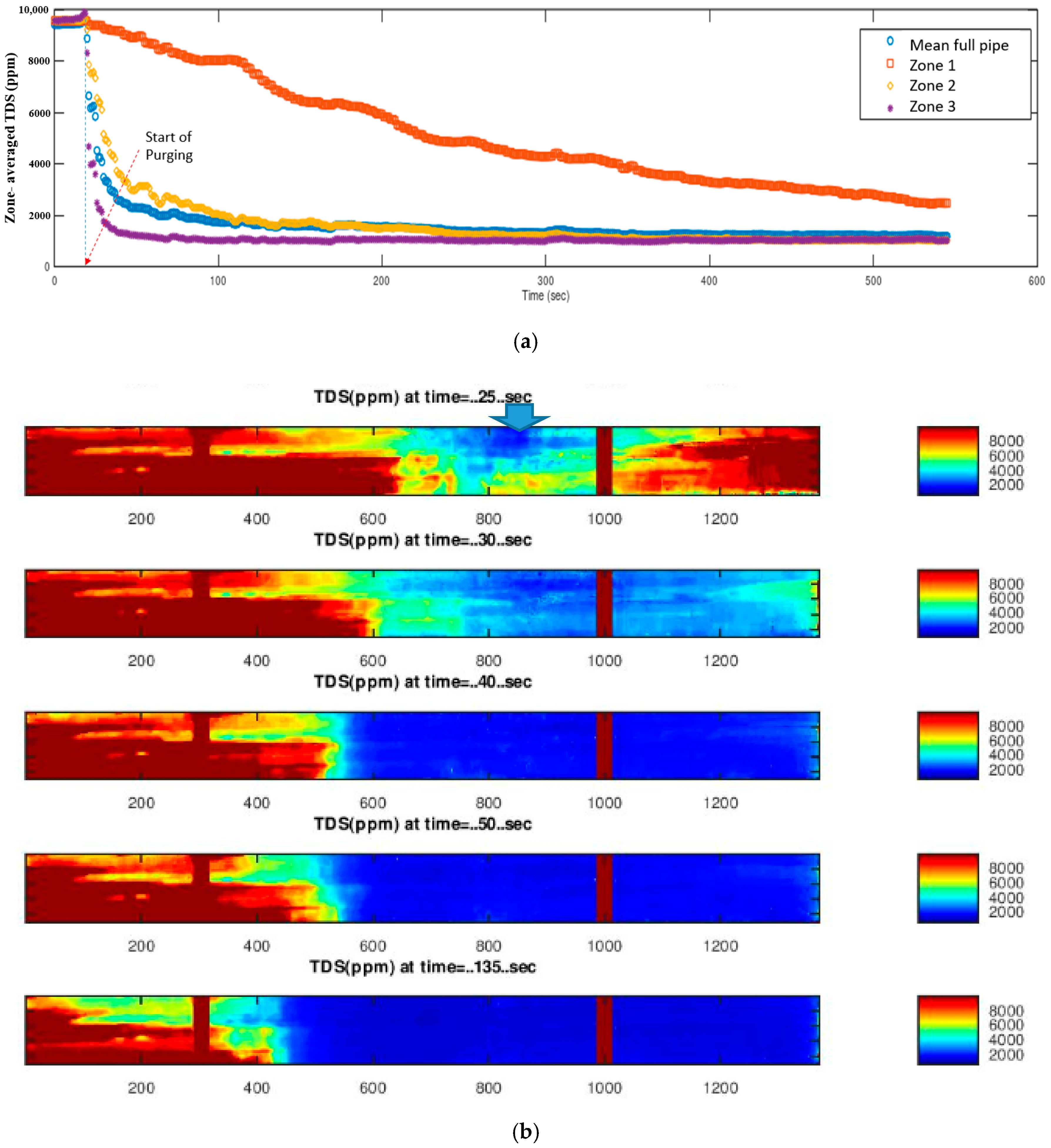
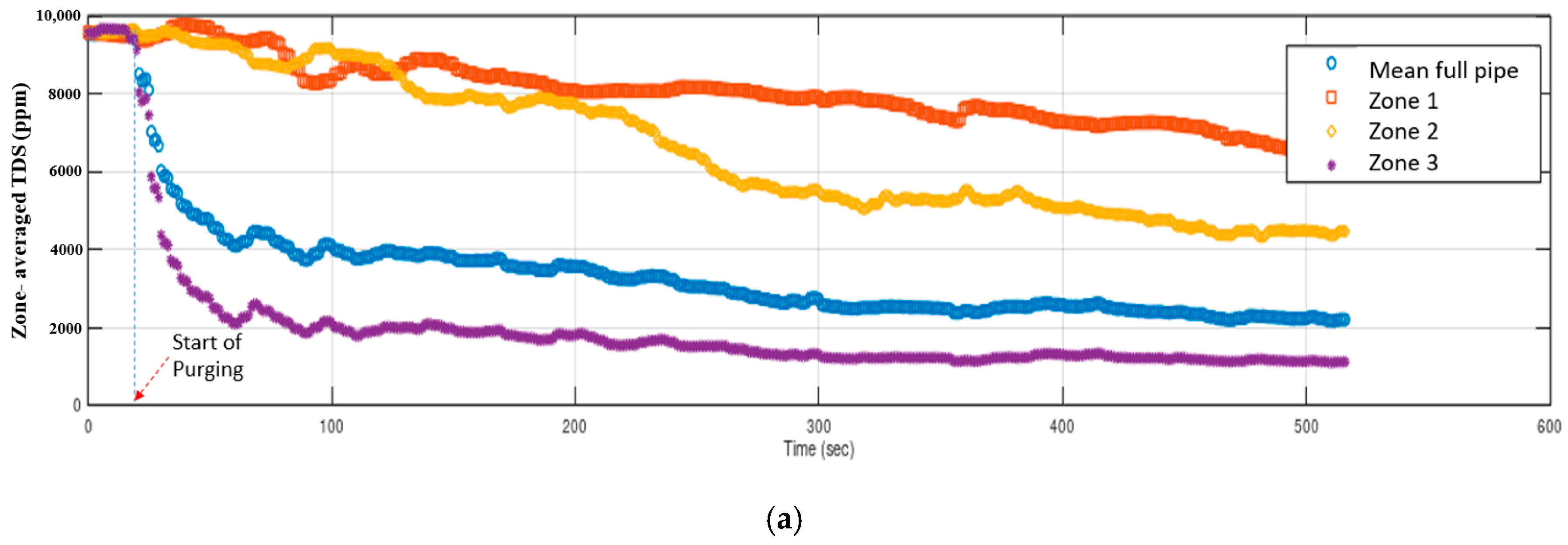
Despite of the effort done to avoid having blurred and light glare spots within the study areas, it was noted that during video recording, spots of light streaks appear on the surface of the Pyrex pipe. Figure 3b shows examples of the light streaks that exist in the study area. Figure 3c shows the schematic of the experimental setup whereas Figure 3d illustrates the study domain which identifies the area that will be continuously captured by the camera during the purging process with the time course. Within the study domain there are two blind areas (shown as hatched areas). The blind areas are located at the dead leg pipe holders. Such areas will be excluded from image processing and they will be represented afterward as opaque areas (refer to Figures 5b, 7b, and 9b). For discussion purposes, the study domain of the dead leg pipe is divided into three zones (zone 1, 2, and 3). The areal average value for the TDS for each zone in addition to the mean value for the whole study domain will be calculated with the time course.
2.3. List of Experimental Runs
In order to study the effect of purging location and purging flow rate on the purging process, 24 purging experiment were conducted to study the purging process in the dead leg pipe. Table 2 shows the characteristics of those runs.
Table 2 shows also the corresponding value of the spatial Reynolds number (Rex) for each run which ranges from 6366 to 135,388. Equation (4) defines the spatial Reynolds number; where Xp is the x-distance of the purging location from the dead end, Re is the convention Reynolds number and D is the pipe diameter.
The spatial Reynolds number is defined as:
Rex = Re * (xp/D))
2.4. Apparatus and Software
Digital point and shot camera, with the characteristics given in Table 3, was used to record still images and video clips for digital image processing and analysis.
A GlowGeek professional water quality test meter (TDS in range 0–9990 ppm) was used to measure the TDS value of the saline solution for different dilutions.
Two units of Omega (Float/spring type) in-line flow meters were used to measure the water flow rate that is used for purging the dead leg end pipe. The two flow meter units were set in parallel to allow for high precision flow measurements for both relatively low and high flow rates (flow range from 0 to 100 L per minute).
A pressure transducer (model: Eyourlife universal −150 psi) is connected to the purging pipe manifold to measure the pressure water head of the purging water. The pressure transducer measures the positive and negative pressure relative to atmospheric pressure (i.e., gage pressure or manometric pressure) for the flow that is used to purge the pipe. The pressure transducer is connected to a micro-controller (Arduino chip) that is used to facilitate data acquisition and data display. At the start of each run and before commencement of purging process the pressure transducer is calibrated against the zero-gage atmospheric pressure. The accuracy of the pressure transducer is about 1% Full scale. The pressure transducer is connected to the crest point of the manifold purging pipe before purging pipe bifurcation (Figure 3c).
The pressure transducer is connected to a micro-controller (Arduino-Uno) which captures pressure data and sends it back to the lab top via USB port. It should be mentioned that the used water pressure head is more than the atmospheric pressure, but less than 1 bar.
An open source freeware programming language for scientific computing (GNU Octave) was selected for digital image and video analysis processing. Many researchers consider GNU Octave as a viable alternative to Matlab [17]. In this study, GNU Octave package was used to write an image processing script code to carry out video analysis for the purging process of the dead leg end pipe.
2.5. Main Assumptions
The study in-hand considers the following main assumptions:
- -
- It is claimed that imaging the pipe from outside will reveal a lot of information about the status of water quality in the dead end-leg during the purging process. The paper assumes that imaging the pipe from outside is significantly correlated to the average of what happens throughout the full pipe cross-section.
- -
- No additional measurement system to validate the results for this regard, authors conducted an extended 3D-numerical study for the same problem using ANSYS Fluent package and good agreement obtained [18].
- -
- The study neglected the effect of non-uniformity and unsteadiness in illumination from the used light sources.
- -
- The study also assumes that there is no access to the front of the dead zone (on site) and therefore direct insertion of clear purging water from the front of the dead end is not possible.
- -
- The influence of the pressure level on the purging process is not investigated.
It should also be mentioned that the purging process proposed in the manuscript allows for a temporally rather than final solution to the intrusion of salty groundwater to the system.
2.6. Work Flow
The work flow for each experimental run includes the following steps:
- -
- Filling the dead leg pipe by the saline solution (TDS = 1867 ppm or TDS = 9600 ppm);
- -
- Selecting the purging location by opening the switch valve of one of the three purging pipes (making sure that the remaining purging pipes are closed);
- -
- Start video recording the purging process then start purging saline by using tap water and;
- -
- Convert the recorded mp4 video file to avi file using VLC freeware software [19]. This step is important since most of the video analysis packages (such as SciLab and Octave) can only read avi files;
- -
- The next step is to read the avi file and to carry out video analysis and image processing using a script code compatible with Octave package and was specifically written for this regard (more details to follow);
- -
- The final step is to plot temporal variations of color intensities and corresponding TDS values then to carry out post processing analysis using Excel.
2.7. Removal of Light Streaks
The above-mentioned light streaks need to be removed from images before starting data processing to get accurate results. It should be mentioned that similar problems in different applications were reported in image processing literature. For instance, Reference [20] proposed a technique to remove haze artifacts from images. While [21] proposed a new image processing technique for video rain streak removal. In the study at hand, the locations of the light streaks were identified from the first frame of the video recording (i.e., image frame when the dead leg pipe is initially filled with saline before starting the purging process). The locations of the light streak pixels are determined by using a number of edge functions, then the values of gray intensity at the location of light streaks pixels are replaced by the corresponding averaged values of nearby pixels.
3. Results and Discussion
3.1. Flow Structure and Eddy Formulation
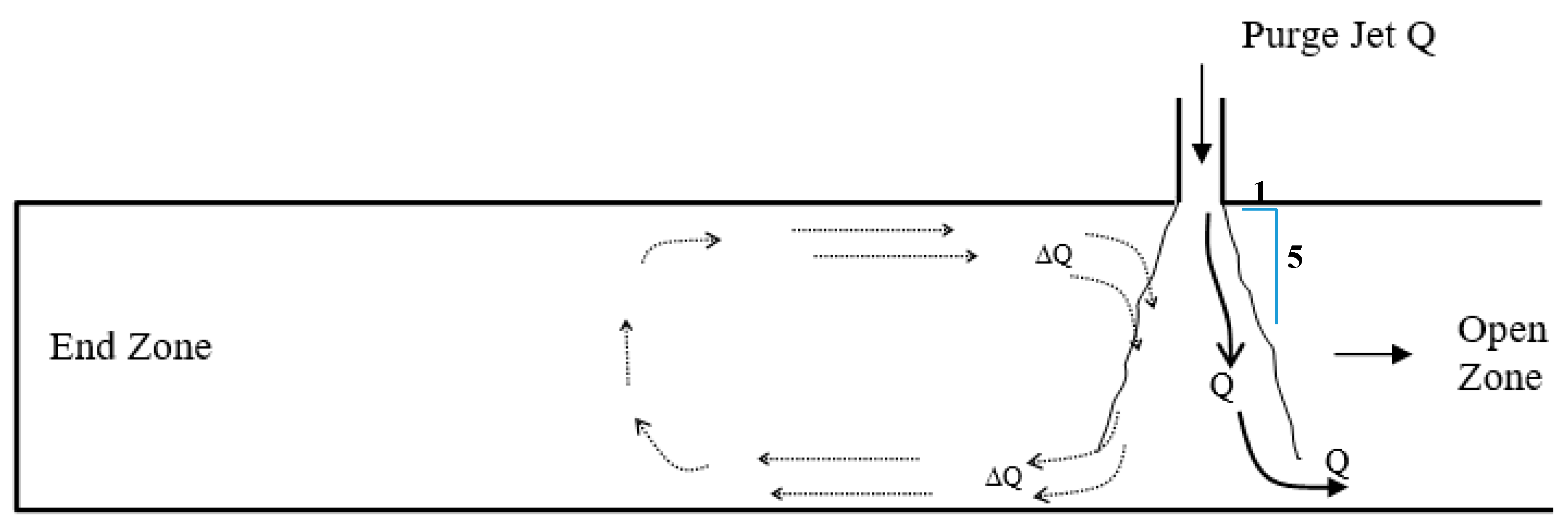
When the purging jet flow enters the pipe, it develops a shear flow zone within the pipe at the jet location. As a result of that, turbulence is produced and starts to be diffused by a turbulence to turbulence diffusion-like process since there is no mean flow in the dead-end zone. The purging jet expands with an approximate slope of 1:5 [22] till it hits the bottom of the pipe, refer to Figure 4. It might be reasonable to say that, during the jet expansion, the jet entrains resident water from the ambient fluid because of the difference in the pressure. As a result of that, the discharge of the jet increases by ∆Q. When the jet hits the bottom wall of the pipe, it is divided into two unequal parts. One part will move towards the open end of the pipe with the full inlet purging discharge, Q. The other part will be directed towards the closed end with a discharge equals ∆Q. At equilibrium the jet will become asymmetric, the full inlet discharge will go to the open end and the closed end pipe could have a circulating flow similar to what is shown in Figure 4. Actually, this circulating flow is driven by the shear forces which are produced by the sides of the jet. It should be mentioned that although there is a circulating flow in the closed end, the cross-sectional averaged velocity will stay equal to zero to satisfy the mass conservation law.
It has been noted that the density difference (resulted from having TDS variations from 1867 ppm to 9600 ppm) has a marginal effect on the purging process therefore the discussion will be focused on the results from runs 11 to 24 that has an initial TDS of 9600 rpm. Readers interested in the density effect on the purging process can find more details about that subject in Reference [19].
3.2. First Purging Location (Xp/D = 3)
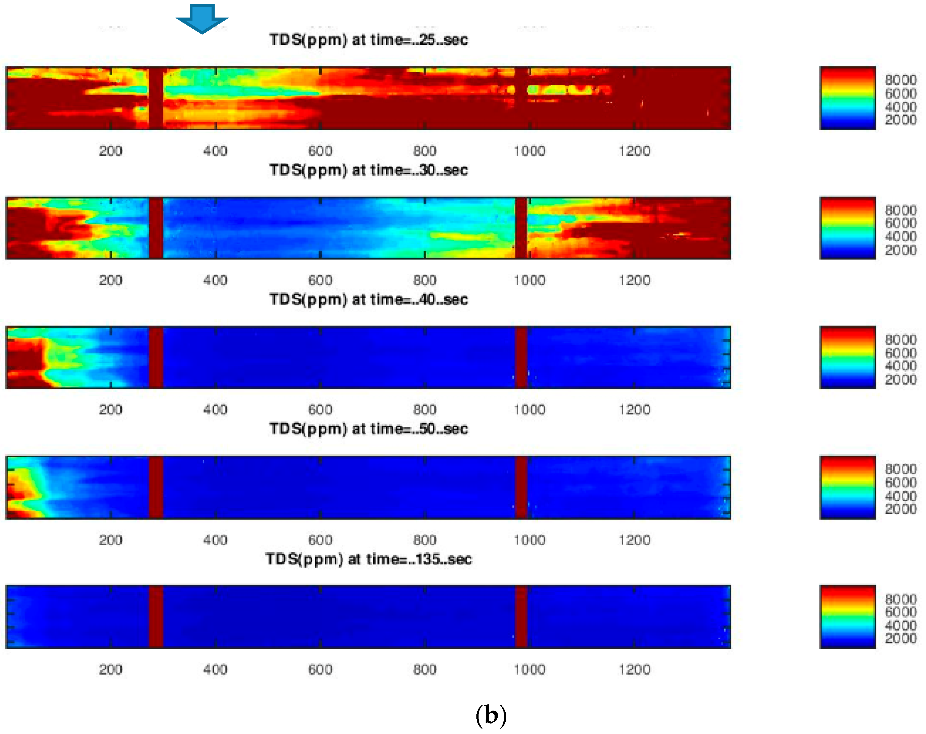
Figure 5, shows the results of the purging process through purging location number 1 (while purging locations number 2 and 3 are kept closed) with the purging flow rate of 59 L/min, as per Run#12. The temporal reduction of TDS in the dead leg pipe with the course of time is shown in Figure 5a.
Figure 6a shows that the purging commences after about 20 s from the start of video recording and almost 95% of complete removal of saline took place at about 135 s from the start of recording (115 s from the start of purging). It is noted that purging of zone 1 in the pipe takes longer to be purged compared to the other zones within the study domain. Figure 6b presents the color maps of TDS and its temporal variation with time. The figure clearly shows that zone 1 is the latest zone to be cleaned from saline compared to other zones.
A time scale ts is introduced to present the time data in a normalized way. The time scale represents the time required to fill an empty pipe of length L and diameter D using an input flow rate equals the purging flow rate. The time scale is therefore defined as:
ts = (πLD2/4Q)
The time spent since the start of purging is defined as t and is given as:
where T is the time course from the start of image recording and to is the initial time of purging
t = T − to
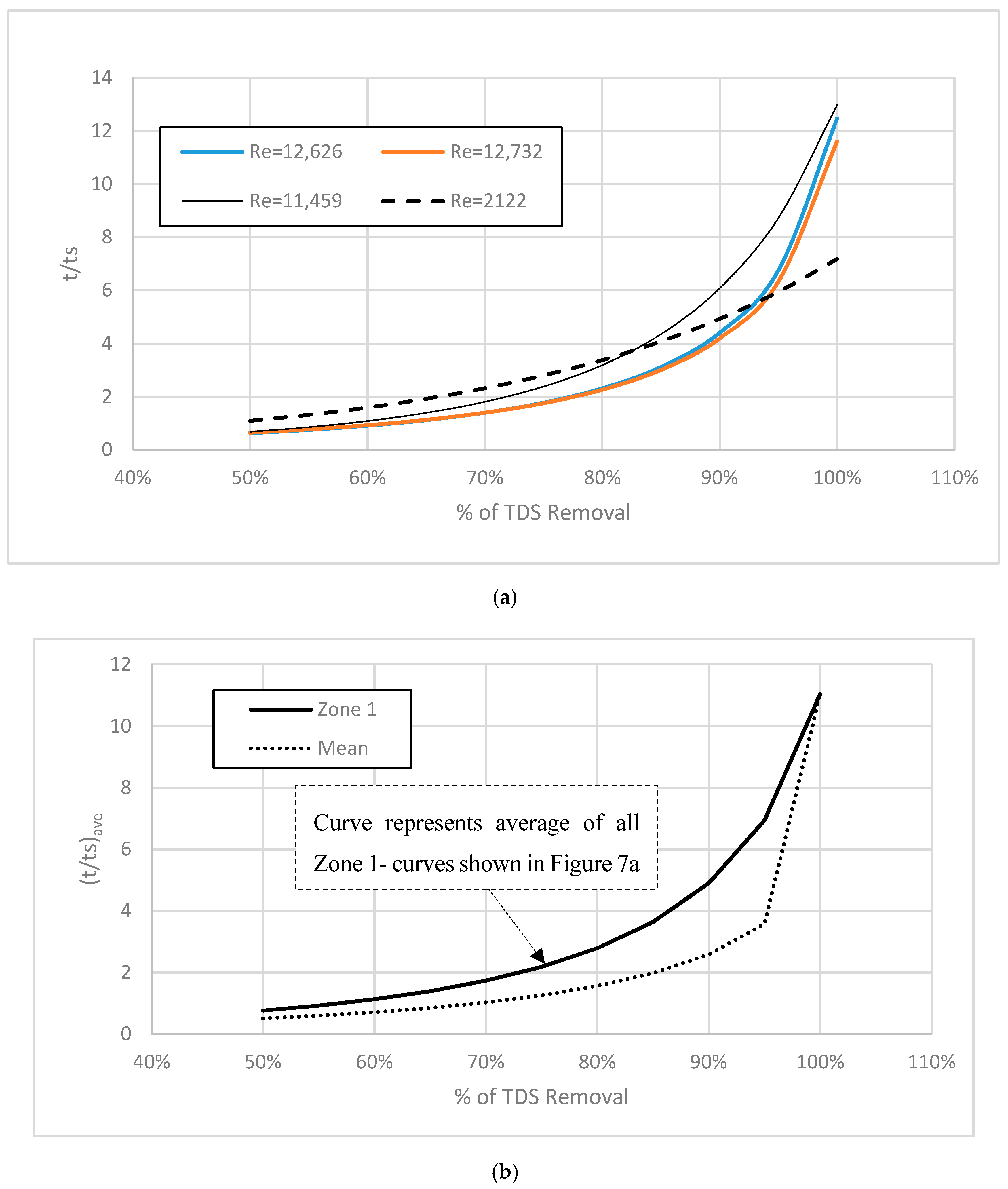
Figure 6a shows the effect of applying different purging flow rates (i.e., different Re) on the time of removal ratio (t/ts) for zone 1. This figure summarizes the results of Runs#11 to 14. It is interesting to note that high purging flow rate (i.e., high Re value) seems to have faster removal capability initially. On the contrary, a low purging flow rate seems to have slower removal capability initially, but faster removal capability eventually.
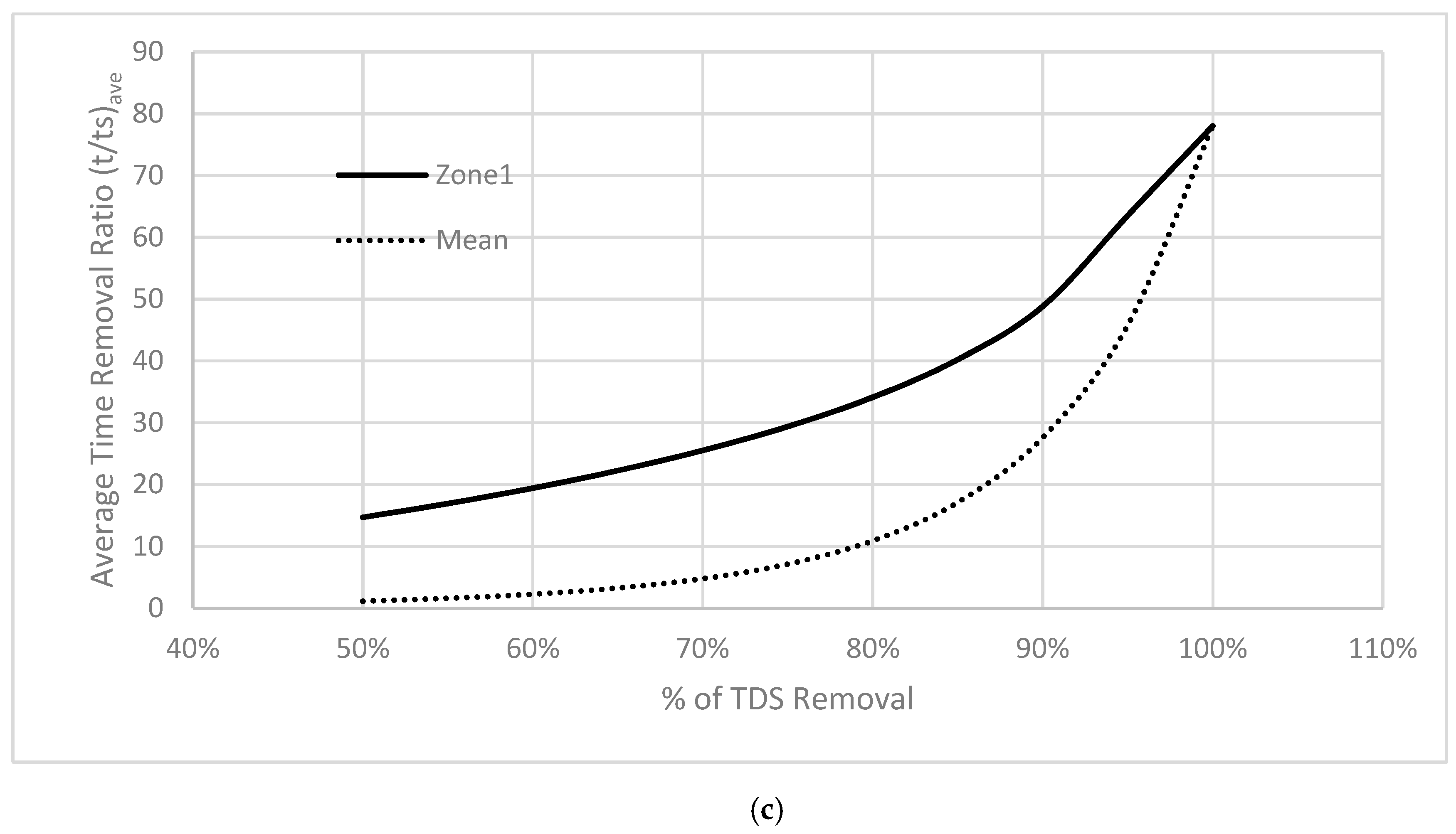
Figure 6b summarizes the output of experiments conducted for purging location #1. It presents the average purging time ratio required to reach a specified TDS removal percentage. It is clear that Zone 1 (solid line curve) requires more time for TDS removal compared to the average of the whole study domain (dotted line curve). For instance, Figure 6b shows that to achieve 90% of TDS removal in Zone 1, purging need to be conducted (at purging location #1) for time equals about 4.9 times the time scale (ts). Figure 6b also shows that complete removal of TDS requires purging at purging location #1 for at least 11 times the time scale (ts).
3.3. Second Purging Location (Xp/D = 7)
Figure 7a,b summarize of the result of run #15 for the mid-purging pipe (number 2) that is located about 7 times the pipe diameter from the dead leg end of the pipe (i.e., purging location = 7D). In this run, the purging flow is about 60.5 L/min. Figure 8a shows that TDS was reduced by 50% in zone 1 after 230 s.
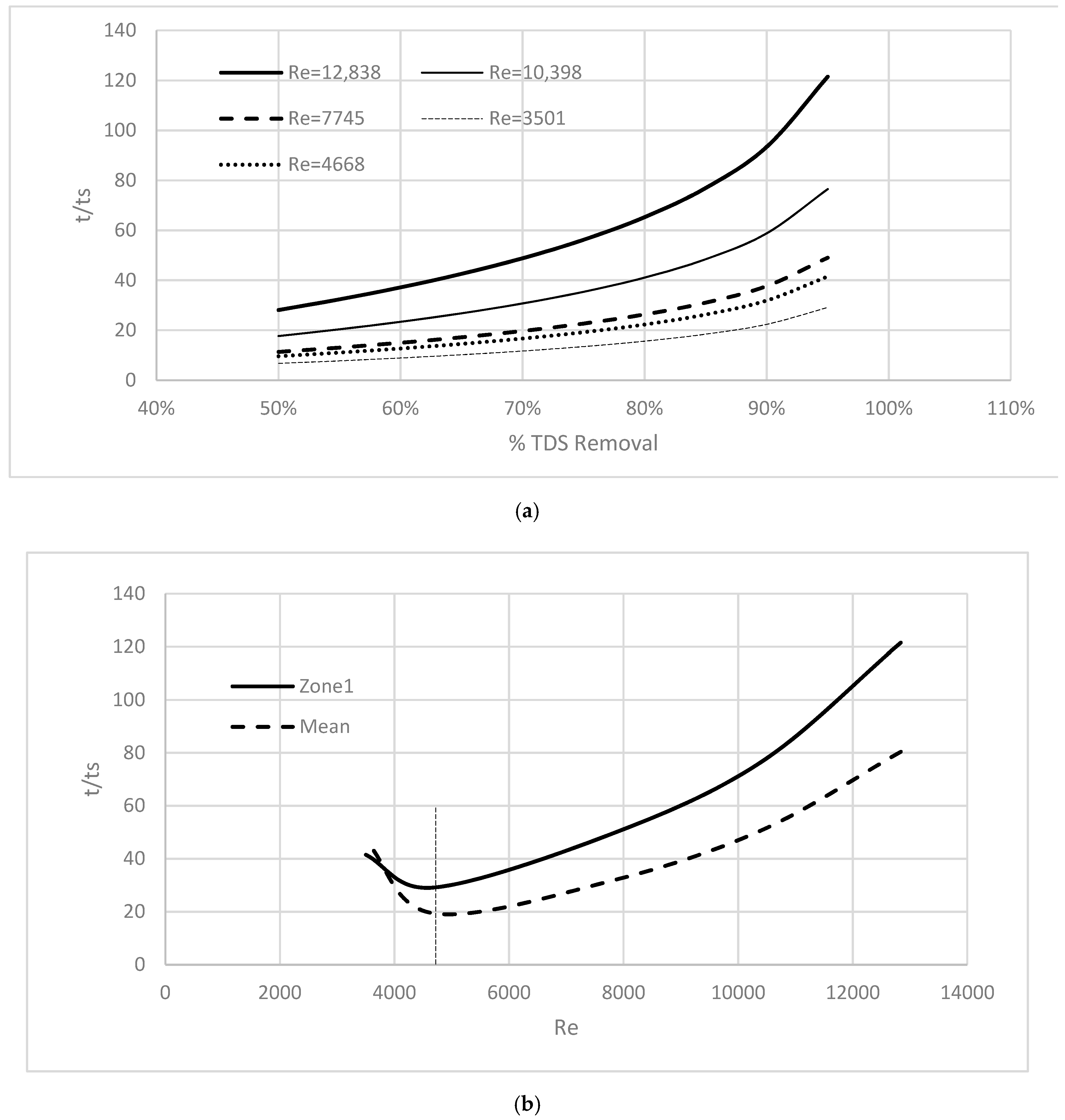
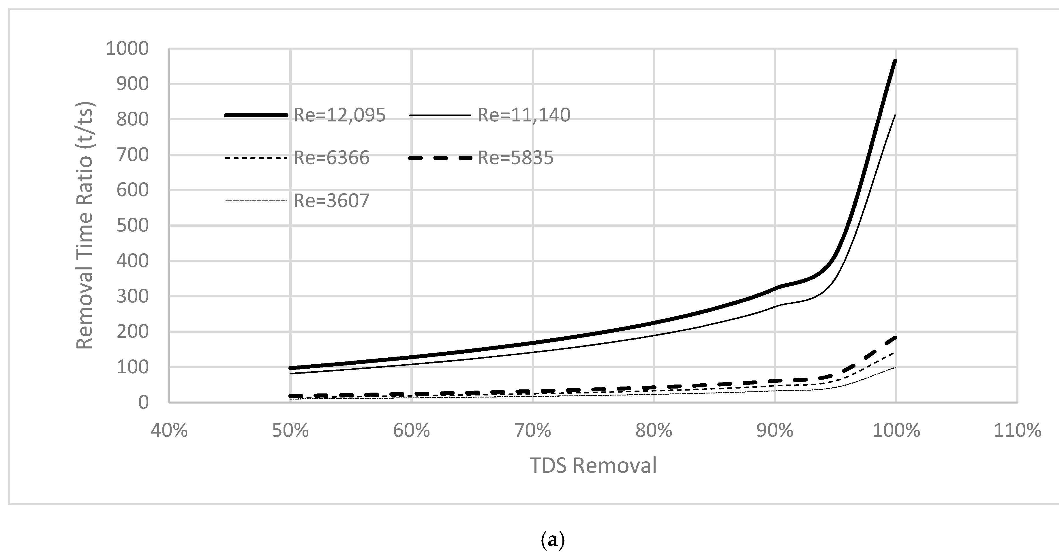
Figure 8a shows the effect of using different purging flow rates (i.e., different Re) on the time of removal ratio. This figure summarizes the results of Runs#15 to 19. It is interesting to note that low purging flow rate (i.e., low Re values) seems to generally have a smaller time removal ratio compared to high purging flow rate. It should be mentioned that as Re increases purging flow velocity increases resulting in smaller value of time scale ts and thus a larger value of t/ts. Figure 8b shows that purging at Re equals 4668 will result in the minimum t/ts ratio to achieve 95% TDS removal.
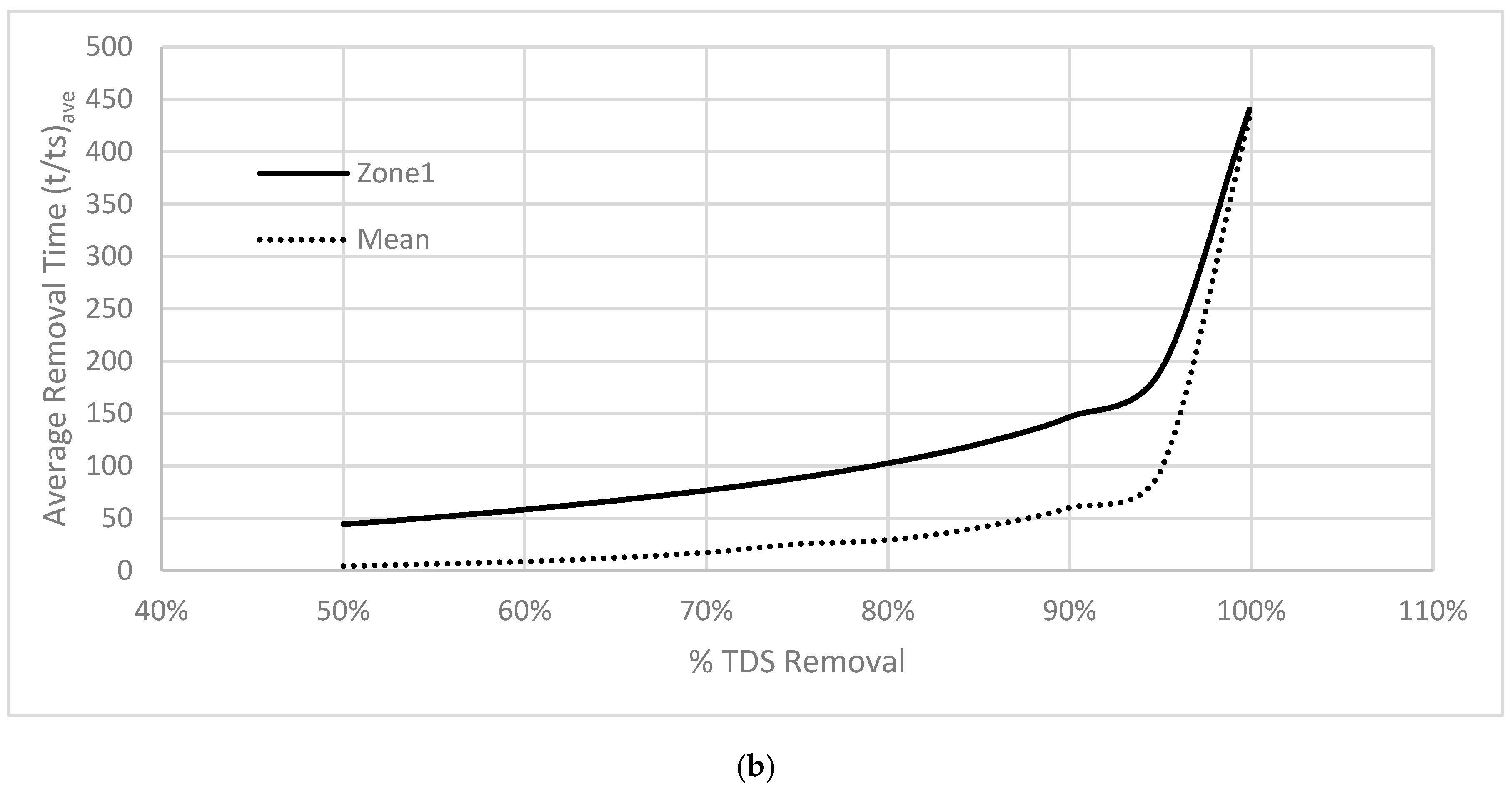
Figure 8c summarizes the output of experiments conducted for purging location #2. It presents the average purging time ratio required to reach a specified TDS removal percentage. It is clear that Zone 1 (solid line curve) requires more time for TDS removal compared to the whole study domain (dotted line curve). For instance, Figure 8c shows that to achieve 90% of TDS removal in Zone 1, purging need to be conducted (at purging location #2) for time equals 33 times the time scale (ts). The figure also shows that complete removal of TDS requires purging at purging location #2 for at least 78 times the time scale (ts).
3.4. Third Purging Location (Xp/D = 11)
Figure 9a,b show the temporal reduction of TDS and its color map along the pipe, respectively, in case of applying the purging process from the farthest purging location #3.
Figure 9a,b summarize the result of Run#20 in which the purging point is located about 11 times the pipe diameter from the dead leg end of the pipe. In this run, purging is conducted via the third-purging pipe and the purging flow is about 57 L/min. Figure 10a shows that purging commences after about 20 s of the start of video recording, and after 500 s, the achieved percentage of TDS removal was less than 35% for zone 1.
Figure 10a shows the effect of using different purging flow rates (i.e., different Re) on the time of removal ratio. This figure summarizes the results of Run#20 to 24. It is interesting to note that low purging flow rate (i.e., low Re values) seems to have significantly smaller removal time ratio compared to high purging flow rate.
Figure 10b summarizes the output of experiments conducted for purging location #3. It presents the average purging time ratio required to reach a specified TDS removal percentage. It is clear that Zone 1 (solid line curve) requires more time for TDS removal compared to the whole study domain (dotted line curve). Figure 10b also shows that complete removal of TDS requires purging at purging location #3 for at least 440 times the time scale (ts).
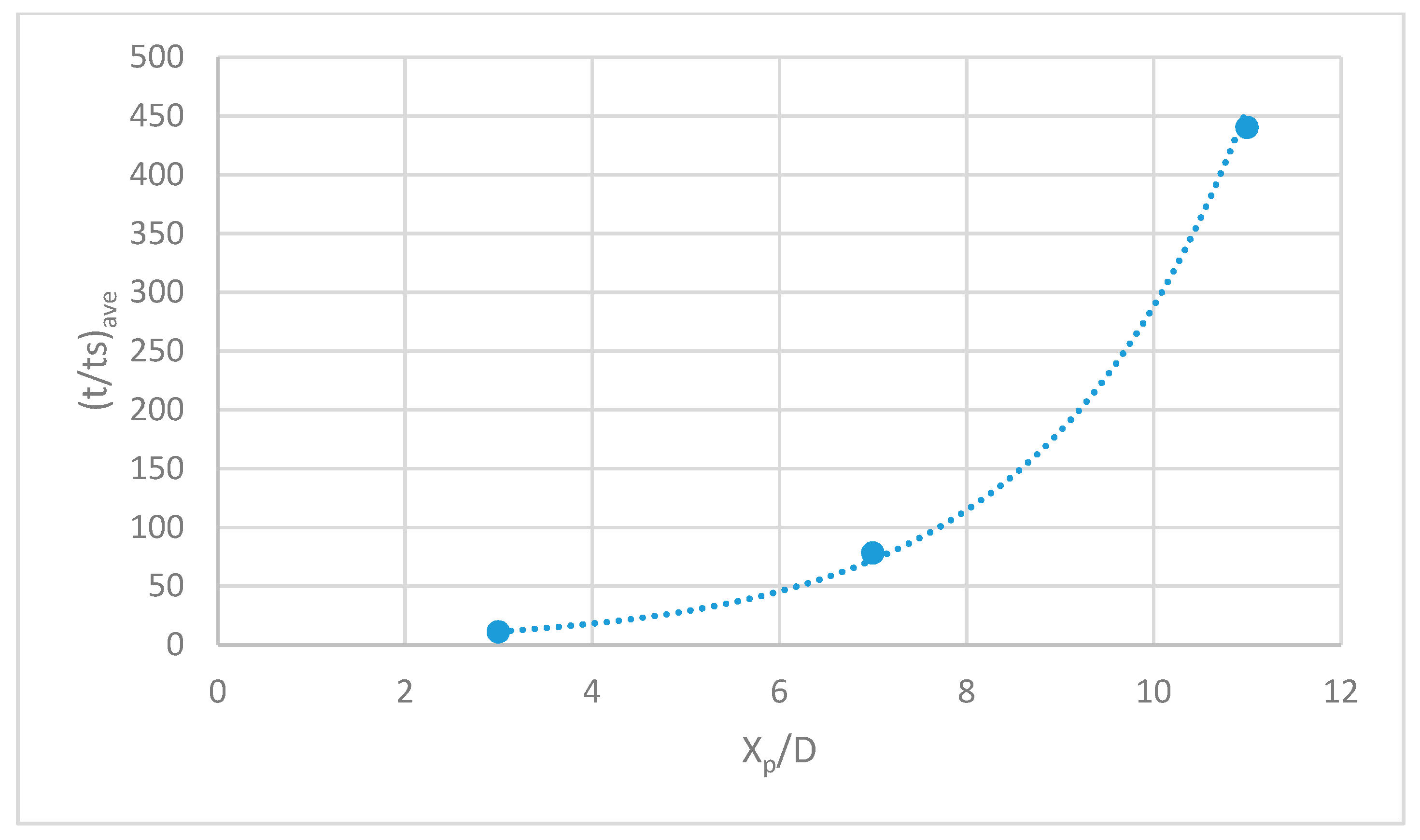
Based on Figure 6, Figure 8, and Figure 10, the dependence of the removal time ratio on the purging location could be formulated as shown in Figure 11. It is clear that as purging location increases (from the dead end) the average removal time ratio to achieve complete removal increases exponentially, as shown in Equation (7).
(t/ts)ave = 2.8653e0.4611(Xp/D)
4. Conclusions and Challenges
In this study, the process of purging saline water from a dead-end water pipe was investigated experimentally. A closed upstream end Pyrex pipe with multiple lateral purging inlets was initially filled with saline water, then tap water was pumped into the pump at one of the purging locations to purge the saline water. The purging process was visually studied using high resolution camera. A saline solution standard was prepared and colored with blue ink then diluted successively to different solute concentration. A number of RGB color matrices were produced and used to construct a universal color intensity-to-salinity conversion curve that relates the color intensity value with the measured solute concentration (TDS).
The study in hand showed that video analysis and image processing are powerful tools that helped much in studying the purging process and in identifying the important factors affecting it. The study generally showed that as Reynolds number of the purging flow increases, the removal time ratio (t/ts) increases too. It was also found that the location of purging significantly affects the time required to achieve complete removal of TDS. As the distance of purging location (from the dead end) increased, the removal time ratio increased exponentially.
Applying the proposed purging process on site might be a challenging. One of the common expected challenges is to avoid salty water to get pushed into the main supply system, the common practice to be followed for this situation is to isolate the area to be purged from the remaining pipeline network system by using the isolation valve that is located downstream to the dead end. Then to open the washout valve just upstream of the isolation valve to allow for drainage of the salty water out of the system. Another challenge is the selection of the purging location. The common practice is to use the fire hydrant as a drainage and wash out of the network. The closest fire hydrant to the end-point should be selected as the time of complete purging exponentially increases with the distance to the dead-end. A third challenge will exist if the contaminant that is intruded into the network is not just saline water, but rather contaminated sewage groundwater. This challenge requires a special study to examine the removal efficiency of such organic and microbial contaminants.
Author Contributions
Conceptualization, M.E. and M.F.; methodology, M.E. and M.F.; software, M.E.; formal analysis, M.E. and M.F.; investigation, M.E. and M.F.; writing—original draft preparation, M.E.; writing—review and editing, M.E. and M.F.; funding acquisition, M.E. and M.F.
Funding
This research received no external funding.
Acknowledgments
The authors would like to thank Eng. Lotfi Chaouachi at Imam Mohamad University for preparing the experimental setup. The authors would also like to thank Maryam Elgamal for editing and punctuating the text of this manuscript.
Conflicts of Interest
The authors declare no conflict of interest.
Abbreviations
| d | Diameter of the inlet purging pipe (d = 1 inch) |
| D | Diameter of the Pyrex pipe to be purged (D = 4 inches) |
| Gr | Grayness ratio, equation 1 |
| Grayi | The gray intensity of the water solution inside the pipe to be purged at any moment I (after commencement of purging) |
| Graym | The initial maximum gray intensity of the saline water (before purging starts) |
| Grayo | The average gray intensity of the tap water |
| GRB | Green-red-blue |
| GNU | is a free licensed operating system that stands for “GNU’s Not Unix!” |
| L | Length of the studied flow domain for the Pyrex pipe (L = 120 cm) |
| mL | Milliliters |
| ppm | Particles per million |
| Q | Purging flow rate |
| Re | Reynolds number of purging flow [Re = 4Q/(πDv)] where v is the kinematic viscosity of the purging fluid |
| Rex | Spatial Reynolds number, equation 4 |
| Sr | Salinity ratio, equation 2 |
| SSS | Saline solution standard |
| T | Time in seconds since start of recording |
| TDS | Total Dissolved Salt (units in ppm) |
| TDSi | The average TDS value of eater solution at any pixel inside the pipe and at any moment I after commencement of purging process |
| TDSm | Maximum TDS value of the solute (before dilution) (TDSm = 1867, 9600 and 14420 ppm for the three solutions) |
| TDSo | The average TDS value of original tap water before adding salt to it (TDSo = 300 ppm) |
| t | Time in seconds since start of purging process, equation 6 |
| to | Time for initiation of purging process |
| ts | Time scale = (πLD2/4Q) and it represents the time required to fill an empty pipe of length L and diameter D for an input flow rate equals the purging flow rate. |
| t/ts | The time ratio or the normalized time required to attain a specified TDS removal percentage |
| (t/ts)ave | The average time of removal ratio calculated to average the value for different purging flow rate |
| UDF | Uni-directional flushing of water network. |
| xp | The distance from the pipe dead end to the purging location and it is measured horizontally, Equation (4) |
| ∆Q | Entrained flow from resident saline water to the purging jet, Figure 4. |
References
- Carter, J.T.; Lee, Y.; Buchberger, S.G. Correlations between travel time and water quality in a dead-end loop. In Proceedings of the Water Quality Technology Conference, American Water Works Association, Denver, CO, USA, 9–12 November 1997. [Google Scholar]
- Galvin, R. Eliminate Dead-End Water. Opflow. 2011. Available online: http://midwestwatergroup.com/ownloads/Opflow%20-%20November%202011%20-%20Dead%20End%20Danger%20Zones.pdf (accessed on 12 March 2019).
- McVay, R.D. Effective Flushing Techniques for Water Systems. Florida Rural Water Association. Available online: http://www.frwa.net/uploads/4/2/3/5/42359811/effectiveflushingtechniquesforwatersystems051608.doc (accessed on 9 April 2019).
- MassDEP, Massachusetts Department of Environmental Protection Drinking Water Program. Fact Sheet Water Main Flushing FAQ for Consumers. 2018. Available online: https://www.mass.gov/files/documents/2018/05/07/Water%20Main%20Flushing%20-%20Fact%20Sheet%20-%20FAQ%20for%20Consumers.pdf (accessed on 6 April 2019).
- Kammereck, L.; Reisinger, D. Flushing Tips: Implementing Unidirectional Flushing Program. Water Finance and Environment, 2016. Available online: https://waterfm.com/implement-unidirectional-flushing-program-improve-efficiency-conservation/ (accessed on 9 April 2019).
- Yuan, W. Practical Analysis of Cleaning Water Supply Pipeline Using Air and Water Flushing Technology. In Proceedings of the 1st International WDSA/CCWI 2018 Joint Conference, Kingston, ON, Canada, 23–25 July 2018. [Google Scholar]
- Barbeau, B.; Gauthier, V.; Julienne, K.; Carriere, A. Dead-end flushing of a distribution system: Short and long-term effects on water quality. J. Water Supply Res. Technol. Aqua 2005, 54, 371–383. [Google Scholar] [CrossRef]
- Ilaya-Ayza, A.; Martins, C.; Campbell, E.; Izquierdo, J. Implementation of DMAs in Intermittent Water Supply Networks Based on Equity Criteria. Water 2017, 9, 851. [Google Scholar] [CrossRef]
- Choe, K.; Varley, R.C.G.; Bijlani, H.U. Coping with Intermittent Water Supply, Problems and Prospects, Environmental Health Project. Activity Report No. 26; Dehra Dun, India, 1996. Available online: https://pdf.usaid.gov/pdf_docs/pnabz958.pdf (accessed on 18 March 2019).
- PNGRB, Petroleum and Natural Gas Regulatory Board, New Deli, India. Available online: http://www.pngrb.gov.in/pdf/public-notice/guidelines22122015.pdf (accessed on 11 may 2019).
- Firdausa, L.; Alwib, W.; Trinoveldib, F.; Rahayuc, I.; Rahmidard, L.; Warsito, K. Determination of Chromium and Iron Using Digital Image-based Colorimetry. Procedia Environ. Sci. 2014, 20, 298–304. [Google Scholar] [CrossRef] [Green Version]
- Fox, S.; Shepherd, W.; Collins, R.; Boxall, J. Experimental Quantification of Contaminant Ingress into a Buried Leaking Pipe during Transient Events. J. Hydraul. Eng. 2016, 142. [Google Scholar] [CrossRef]
- Choodum, A.; Kanatharana, P.; Wongniramaikul, W.; Daeid, N. Using the iPhone as a device for a rapid quantitative analysis of trinitrotoluene in soil. Talanta 2013, 115, 143–149. [Google Scholar] [CrossRef]
- Elgamal, M.; Abdel-Mageed, N.; Helmy, A.; Ghanem, A. Hydraulic performance of sluice gate with unloaded upstream rotor. Water SA 2017, 43, 563–572. [Google Scholar] [CrossRef]
- Stahel, A. Octave and MATLAB for Engineers; Bern University of Applied Sciences: Bern, Switzerland, 2018; Available online: https://web.ti.bfh.ch/~sha1/Labs/PWF/Documentation/OctaveAtBFH.pdf (accessed on 12 March 2019).
- Sony RX100 Cyber-Shot, Instruction Manual. Available online: https://www.docs.sony.com/release/DSCRX100_EN_ES.pdf (accessed on 12 March 2019).
- Coman, E.; Brewster, M.; Popuri, S.; Raim, A.; Gobbert, M. A Comparative Evaluation of Matlab, Octave, FreeMat, Scilab, R, and IDL on Tara. Technical Report HPCF-2012-15. Available online: www.umbc.edu/hpcf (accessed on 12 March 2019).
- Farouk, M.; Elgamal, M.H. CFD Simulation of Flushing the Dead-Ends of a Distribution System, submitted to Water SA. (unpublished).
- VLC for Dummies. Available online: https://wiki.videolan.org/Documentation:VLC_for_dummies/ (accessed on 12 March 2019).
- Yeh, K.C.; Kang, L.W.; Lee, M.S.; Lin, C.Y. Haze effect removal from image via haze density estimation in optical model. Opt. Express 2013. [Google Scholar] [CrossRef]
- Jiang, T.; Huang, T.; Zhao, X.; Deng, L.; Wang, Y. FastDeRain: A Novel Video Rain Streak Removal Method Using Directional Gradient Priors. IEEE Trans. Image Process. 2018, 8, 2089–2102. [Google Scholar] [CrossRef] [PubMed]
- Rajaratnam, N. Turbulent Jets; Elsevier: Amsterdam, The Netherlands, 1976. [Google Scholar]
Figure 1.
RGB Color matrix for SSS after successive dilution (initial salinity of 9600 ppm).

Figure 2.
Gray Intensity-to-Salinity Calibration Curve.

Figure 3.
Experimental Setup. (a) Lab. Experiment Setup; (b) Light streaks (zoom in of dashed frame shown in Figure 3a); (c) Schematic of Experimental Setup; (d) Study domain and different pipe zones for the dead leg pipe.
Figure 3.
Experimental Setup. (a) Lab. Experiment Setup; (b) Light streaks (zoom in of dashed frame shown in Figure 3a); (c) Schematic of Experimental Setup; (d) Study domain and different pipe zones for the dead leg pipe.


Figure 4.
Sketch of flow circulation within the closed end (multiple circulating eddies driven by the purging jet might form).
Figure 4.
Sketch of flow circulation within the closed end (multiple circulating eddies driven by the purging jet might form).

Figure 5.
(a) Temporal Reduction of TDS (Run#12, Xp/D = 3) and (b) Color maps for TDS variation with the course of time (Run #12, Xp/D = 3).
Figure 5.
(a) Temporal Reduction of TDS (Run#12, Xp/D = 3) and (b) Color maps for TDS variation with the course of time (Run #12, Xp/D = 3).


Figure 6.
(a) Effect of Re and Purging Flow Rate on Time of TDS Removal Ratio (Zone 1, Xp/D = 3) and (b) average Time of Removal Ratio for Achieving a Specified % of TDS Removal (Xp/D = 3).
Figure 6.
(a) Effect of Re and Purging Flow Rate on Time of TDS Removal Ratio (Zone 1, Xp/D = 3) and (b) average Time of Removal Ratio for Achieving a Specified % of TDS Removal (Xp/D = 3).

Figure 7.
(a)Temporal Reduction of TDS (Run #15, Xp/D = 7) and (b) color maps for TDS variation with the course of time (Run #15, Xp/D = 7).
Figure 7.
(a)Temporal Reduction of TDS (Run #15, Xp/D = 7) and (b) color maps for TDS variation with the course of time (Run #15, Xp/D = 7).

Figure 8.
(a) Effect of Re and Purging Flow Rate on Time of TDS Removal Ratio (Zone 1, Xp/D = 7); (b) effect of Re and Purging Flow Rate on Time of Removal Ratio (%TDS Removal = 95%, Xp/D = 7); and (c) average Time of Removal Ratio for Achieving a Specified % of TDS Removal (Xp/D = 7).
Figure 8.
(a) Effect of Re and Purging Flow Rate on Time of TDS Removal Ratio (Zone 1, Xp/D = 7); (b) effect of Re and Purging Flow Rate on Time of Removal Ratio (%TDS Removal = 95%, Xp/D = 7); and (c) average Time of Removal Ratio for Achieving a Specified % of TDS Removal (Xp/D = 7).


Figure 9.
(a) Temporal Reduction of TDS (Run#20, Xp/D = 11) and (b) color maps for TDS variation with the course of time (Run #20, Xp/D = 11).
Figure 9.
(a) Temporal Reduction of TDS (Run#20, Xp/D = 11) and (b) color maps for TDS variation with the course of time (Run #20, Xp/D = 11).


Figure 10.
(a) Effect of Re and Purging Flow Rate on Time of TDS Removal Ratio (Zone 1, Xp/D = 11) and (b) average Time of Removal Ratio for Achieving a Specified % of TDS Removal (Xp/D = 11).
Figure 10.
(a) Effect of Re and Purging Flow Rate on Time of TDS Removal Ratio (Zone 1, Xp/D = 11) and (b) average Time of Removal Ratio for Achieving a Specified % of TDS Removal (Xp/D = 11).


Figure 11.
Effect of Purging Location on the Average Time of Removal Ratio to Achieve Complete TDS Removal.
Figure 11.
Effect of Purging Location on the Average Time of Removal Ratio to Achieve Complete TDS Removal.


Table 1.
Universal constants of Equation (3).
| Constant | a | b | c | d |
|---|---|---|---|---|
| Value | −4.39063 | 2.809594 | −0.7372 | 0.996435 |
Table 2.
Characteristics of the Conducted Experimental Runs.
| Run # | Run ID | Purging Flow(L/min) | Reynolds No (Re) | Purging Distance Ratio (Xp/D) | Spatial Reynolds No (Rex) | Purging Location | Initial Salinity of Purged Solution (ppm) | |||
|---|---|---|---|---|---|---|---|---|---|---|
| 1 | 2 | 3 | 1867 | 9600 | ||||||
| 1 | PPM1867Inj1Q1 | 60.8 | 12,902 | 3 | 38,706 | √ | √ | |||
| 2 | PPM1867Inj1Q2 | 10 | 2122 | 3 | 6366 | √ | √ | |||
| 3 | PPM1867Inj1Q3 | 10 | 2122 | 3 | 6366 | √ | √ | |||
| 4 | PPM1867Inj2Q1 | 56 | 11,884 | 7 | 83,188 | √ | √ | |||
| 5 | PPM1867Inj2Q2 | 46 | 9762 | 7 | 68,334 | √ | √ | |||
| 6 | PPM1867Inj2Q3 | 14 | 2971 | 7 | 20,797 | √ | √ | |||
| 7 | PPM1867Inj3Q1 | 60 | 12,732 | 11 | 140,052 | √ | √ | |||
| 8 | PPM1867Inj3Q2 | 58 | 12,308 | 11 | 135,388 | √ | √ | |||
| 9 | PPM1867Inj3Q3 | 46 | 9762 | 11 | 107,382 | √ | √ | |||
| 10 | PPM1867Inj3Q4 | 12 | 2546 | 11 | 28,006 | √ | √ | |||
| 11 | PPM9600Inj1Q1 | 59.5 | 12,626 | 3 | 37,878 | √ | √ | |||
| 12 | PPM9600Inj1Q2 | 59 | 12,520 | 3 | 37,560 | √ | √ | |||
| 13 | PPM9600Inj1Q3 | 54 | 11,459 | 3 | 34,377 | √ | √ | |||
| 14 | PPM9600Inj1Q4 | 10 | 2122 | 3 | 6366 | √ | √ | |||
| 15 | PPM9600Inj2Q1 | 60.5 | 12,838 | 7 | 89,866 | √ | √ | |||
| 16 | PPM9600Inj2Q2 | 49 | 10,398 | 7 | 72,786 | √ | √ | |||
| 17 | PPM9600Inj2Q3 | 36.5 | 7746 | 7 | 54,222 | √ | √ | |||
| 18 | PPM9600Inj2Q4 | 22 | 4669 | 7 | 32,683 | √ | √ | |||
| 19 | PPM9600Inj2Q5 | 16.5 | 3501 | 7 | 24,507 | √ | √ | |||
| 20 | PPM9600Inj3Q1 | 57 | 12,096 | 11 | 133,056 | √ | √ | |||
| 21 | PPM9600Inj3Q2 | 52.5 | 11,141 | 11 | 122,551 | √ | √ | |||
| 22 | PPM9600Inj3Q3 | 30 | 6366 | 11 | 70,026 | √ | √ | |||
| 23 | PPM9600Inj3Q4 | 27.5 | 5836 | 11 | 64,196 | √ | √ | |||
| 24 | PPM9600Inj3Q5 | 17 | 3608 | 11 | 39,688 | √ | √ | |||
Table 3.
Characteristics of Used Camera [16].
Table 3.
Characteristics of Used Camera [16].
| Digital Camera Model: | Sony RX100 Cyber-Shot |
|---|---|
| Camera Maximum Resolution: | 20.1 Mega Pixel |
| Camera Sensor: | BSI CMOS Sensor |
| Sensor size: | 1” |
© 2019 by the authors. Licensee MDPI, Basel, Switzerland. This article is an open access article distributed under the terms and conditions of the Creative Commons Attribution (CC BY) license (http://creativecommons.org/licenses/by/4.0/).
Share and Cite
MDPI and ACS Style
Elgamal, M.; Farouk, M. Experimental Investigation of Purging Saline Solution from a Dead-End Water Pipe. Water 2019, 11, 994. https://doi.org/10.3390/w11050994
AMA Style
Elgamal M, Farouk M. Experimental Investigation of Purging Saline Solution from a Dead-End Water Pipe. Water. 2019; 11(5):994. https://doi.org/10.3390/w11050994
Chicago/Turabian StyleElgamal, Mohamed, and Mohamed Farouk. 2019. "Experimental Investigation of Purging Saline Solution from a Dead-End Water Pipe" Water 11, no. 5: 994. https://doi.org/10.3390/w11050994
Note that from the first issue of 2016, this journal uses article numbers instead of page numbers. See further details here.