Hydrological Simulation for Karst Mountain Areas: A Case Study of Central Guizhou Province

Abstract

A groundwater model is needed to describe the complex groundwater confluence process of the groundwater system in karst areas. This is because surface water flows through dolines, grikes, and by other means and is directly exchanged with the groundwater. In this study, using the Xin’anjiang model, the conversion of surface water into groundwater and the influence of multiple series-parallel underground reservoirs on groundwater confluence through the generalization of dolines in karst areas were simulated. The water cycle process in the Sancha River Basin was simulated with measured data using multiobjective particle swarm optimization. Then, model parameters were validated with measured runoff data and compared with simulation results obtained using the traditional Xin’anjiang model based on its optimal parameters. The results showed that the determination coefficients of all hydrological stations over the study period were >0.76, and the Nash efficiency coefficient was >0.76, which were better than those for the improved Xin’anjiang model. Next, the simulation accuracy of the flood period in the karst area was analyzed. The model achieved a high fitting rate for the main flood peaks in a year, and the passing rate for the worst hydrological stations was 53%. Finally, the influence of karst development on the runoff was examined. The results indicate that different karst development stages and the heterogeneity of the karst in the basin have different effects on runoff.

1. Introduction

Karst aquifers represent approximately 12% of the continental area of Earth. Approximately 25% of the global population uses drinking water from these hydrogeological systems [1]. Karst aquifers differ significantly from other aquifers because of their complex and unique characteristics [2]. Physical and chemical processes, including tectonic movements in limestone, dolomite, and other soluble rocks, have formed well-linked fissure systems in karst massifs, with dimensions varying from micrometers to several meters [3]. Water rapidly infiltrates the underground network of karst channels because there is extensive development of dissolution pores, caverns, solutional cavities, and subterranean stream systems, which causes surface-water scarcity [1,4,5,6,7,8].

The recharge source for karst water deep in a mining area is water from higher mountain areas, which is transported via vertical leakage [9]. Surface and subsurface karren, grike, and dissolution pores in karst mountainous areas are abundant [10], causing the runoff coefficient of the slope surface to be lower than that in non-karst areas [11,12,13]. Thus, rainfall rapidly infiltrates the bedrock through discontinuous systems in the soluble rock mass, creating an underground network of conduits and caves, which is the most typical feature of karst environments [14]. To describe the runoff process in a mass-fractured medium, Yurtsever and Payne [15] modeled the nonlinear reservoir characteristics of an aquifer using three parallel linear reservoirs, and they analyzed the environmental tritium contents of the Manavgat River in Turkey. Because karst aquifers are predominantly unconfined, nonlinear reservoir recession was expected. Ebru and Hartmut [16] determined the aquifer characteristics via flow recession analysis, and based on the obtained recession parameters, the karst outflow was separated from the time series of total daily flows. Alon [17] developed a conceptual hydrological model for karst environment (HYMKE) and used it to simulate the runoff process of three tributaries in the upper reaches of the Jordan River (in a karst area). Gilboa [18] used the HYMKE model to predict the Lake Kinneret watershed in the karst area of Israel and obtained good simulation results. Damir [19] coupled a moisture balance model with a groundwater balance model to perform a hydrological simulation of the Jadro Spring Basin. Ivana Zěljković [20] established a simple rainfall-runoff model consisting of two submodels for the Opacac karst spring in Dalmatia (Croatia), and the results demonstrated that the groundwater equilibrium composition in karst areas could be estimated by adding parallel linear reservoirs to the model.

Karst areas in China are generally in mountainous regions, mainly concentrated in the Yun-Gui Plateau and the southwestern part of Sichuan Province [21]. Zhang [22] introduced a hydrological model for karst areas, in which the karst area was treated as a whole, to simulate the runoff processes of surface water and groundwater via systematic analysis. Cheng [23] developed a three-source Xin’anjiang model for karst areas, in which the flow of the karst area was a direct (quick) flow, and groundwater flow was modeled in the form of linear reservoirs. The soil and water assessment tool (SWAT) model is a distributed hydrological model developed by the United States Department of Agriculture (USDA) [24]. Ren [25] modified the SWAT model by using linear reservoirs to depict the regulation mechanism of the grikes network of the Diaohe River Basin. Considering the spatial variabilities of hydrological factors and the interrelation of hydrological cells, Beven and Kirkby [26] proposed the topography-based hydrological model (TOPMODEL) based on variable source flow. Then, Suo [27] improved the TOPMODEL to calculate runoff generation in subcatchments in a karst region. Shi [28] simulated runoff in the karst area of Guizhou Province in southwestern China using the Xin’anjiang model. The results indicated that the Xin’anjiang model was applicable in karst areas, but its accuracy was not high.

Flood disasters are among the most frequent and severe natural disasters in the world. With the deepening of scientific research on climate change and regional sustainable development, changes in flood disaster effects have received increasing attention in the fields of international meteorological, hydrological, and disaster risk [29]. With the background of persistent global climate anomalies since the beginning of the 21st century, annual average economic loss from floods in China has reached nearly 100 billion yuan, and it continues to increase [30]. Floods in karst areas are difficult to simulate accurately using conventional hydrological models [31]. As the economies of the world develop, flood losses are increasing, and there is a shortage of water resources [32].

In summary, most hydrological simulations for karst regions divide the runoff into direct surface flow and groundwater flow, which combine at the basin outlet through the confluence of different forms to model the complete runoff process. However, multiple media such as karrens, grikes, and dissolution pores that exchange runoff between surface water and groundwater are not elaborately reflected in the model structure. The applicability of the method based on the distributed hydrological model for a karst basin is limited because it requires detailed information. However, a lumped hydrological model has reasonable application prospects for a complex watershed in the underlying surface, as there is generalization applied to the overall system.

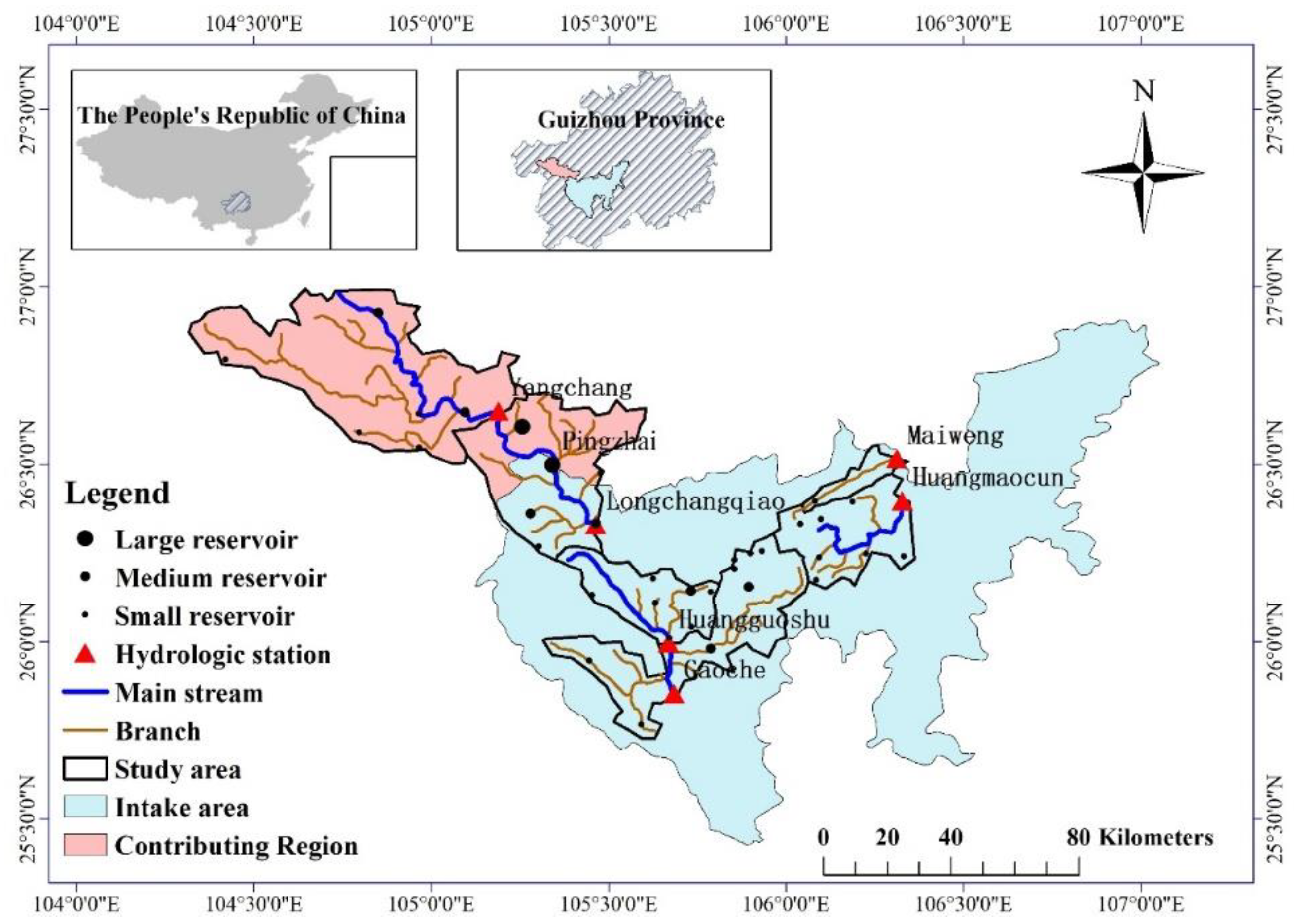
China’s karst landforms are mainly located in the southwestern region and are concentrated in Guizhou Province. The Central Guizhou Province water diversion project is a long-distance, large-scale water transfer and conservancy project located in the karst mountain area of the Sancha River (Figure 1). However, the project is located at the karst hilly area of the Yunnan–Guizhou Plateau, so vigorous development of the karren and subterranean stream system significantly impacts runoff at the exit of the basin. Accurate simulation of the runoff at each hydrological site is very useful to balance and configure the water supply and demand in the project area. In addition, it is necessary to verify the applicability of the model in the flood season and determine whether it can accurately simulate flood peaks. This can provide better assistance and guidance for flood disaster risk management and flood resource utilization in the Central Guizhou Province water diversion project.

We selected the main research area in the Central Guizhou Province water diversion project (i.e., the Sancha River Basin) for hydrological simulation research. The primary objectives of this study were as follows: (a) According to the traditional Xin’anjiang model, a set of methods for simulating the production and confluence of karst areas was established, and the parameters were optimized by applying multiobjective particle swarm optimization (MOPSO) to construct an improved Xin’anjiang model (hereinafter referred to as IXAJ). The daily runoffs from six hydrological stations were simulated using the IXAJ model, and the average monthly runoffs were calculated accordingly. Then, the optimization results were compared with the runoff simulated by the traditional Xin’anjiang model (hereinafter abbreviated as XAJ) with MOPSO. (b) The relative error of the monthly runoff (bias), the coefficient of certainty (R²), and the Nash efficiency coefficient (Nash) were employed to evaluate the simulation results of the IXAJ and XAJ models. (c) The simulation results for the flood period were analyzed using the annual flood peak relative error. (d) Finally, effects of the uneven distribution of the karst development degree and the karst development degree of the runoff in the study area were analyzed.

2. Study Area and Data Material

The Sancha River Basin is located in central Guizhou, the river source zone of two rivers at the watershed, and a karst gorge mountainous area. The project area was located in the central part of Guizhou Province, at the center of the “Zhuliu” double-line economic belt. This is the most densely populated industrial base in Guizhou Province. It is located at the junction of the Yangtze River Basin and the Pearl River Basin. The elevation from the southeast to the northwest (inland direction) gradually increases, reaching 2761 m. After the project was completed, water could be supplied directly to the irrigation district of central Guizhou and the urban areas of Guiyang and Anshun. This could effectively resolve the water shortage in central Guizhou, ensure food security in the irrigation district, improve the quality of life of urban residents, and provide an opportunity to improve the local ecological environment. The project provided an important reference for other areas of Guizhou Province to solve the contradiction between the supply and demand of water resources. The study area was located at the border of the Yangtze River Basin and the Pearl River Basin. There were six hydrological stations and 35 reservoirs in the study area. Regarding the hydrological stations, the Yangchang and Longchangqiao stations were located at the Sancha River, which was the south branch of the Wujiang River. The Maiweng and Huangmaocun stations were located at another tributary of the Wujiang River, which belonged to the Yangtze River Basin. The Huangguoshu and Gaoche stations were located at the Dabanghe River, which belonged to the Pearl River basin. The catchment area and other information of the above hydrological stations are shown in

Table 1. Hydrological stations in study area.

Hydrological Station	River	Drainage Area (km2)	Annual Average Runoff (m3/s)	Precipitation (mm)
Yangchang	Sancha River	2696	42.3	980
Longchangqiao		4327	84.9	1149
Maiweng	Leping River	189	3.89	1228
Huangmaocun	Maotiao River	759	12.5	1168
Gaoche	Dabang River	2264	48.5	1205
Huangguoshu		720	12	1293

. Among the reservoirs, there were 2 large reservoirs, 5 medium-sized reservoirs, and 25 small reservoirs. The watershed above the Pingzhai Reservoir in the basin was the water source area of the project, and the remainder was the water receiving area (Figure 1).

The research period of this paper was from 2000 to 2012, the calibration period was from 2000 to 2008, and the validation period was from 2009 to 2012. Precipitation and evaporation data were provided by the Guizhou Provincial Bureau of Hydrology and Water Resources, including a total of 51 weather stations in the study area. Runoff data were taken from the Chinese Hydrographic Yearbook. The above data were reviewed and had representativeness. Precipitation and evaporation were processed according to the Thiessen polygon to obtain the daily value.

3. Model Structure of the Improved Xin’anjiang Model (IXAJ) Model

In this study, the XAJ model was improved, and the karst regulation and storage processes of groundwater simulation were increased to provide better simulation accuracy in karst areas. The specific description of the improved model (i.e., IXAJ model) was as follows: the runoff generation and division of water sources for the IXAJ model were kept unchanged, that is, the two parts were same as the XAJ model. (The structure of the traditional Xin’anjiang model is detailed in Appendix A.) But the regulation of ground runoff by the clint, doline, etc., was added to the IXAJ model, and the groundwater system was generalized to better simulate the regulation of runoff in karst areas. Finally, conduit flow, surface water, and groundwater were combined into total runoff. The main improvement of the IXAJ model was the groundwater module. The following section focuses on the improvements to the model.

The most typical characteristic of the karst basin is the unique binary three-dimensional (3D) system formed by different types of aqueous media. The key to karst basin hydrological simulation is how to accurately simulate regulation and storage effects of the aquifer medium on the runoff process. Although the aquifer medium is nonhomogeneous and multitudinal, it can be mainly generalized into two classes. The first is the pipeline, including dolines and karst funnels. The flow though pipelines is heavy and usually develops from the surface to the underground or is completely underground. The pipeline from the surface to the underground generally acts as a channel that transports the surface water to the groundwater. Part of the surface water does not experience surface regulation and directly enters the underground to become groundwater runoff, and its main regulation is carried out underground. Because wider pipes transport larger amounts of surface water to the underground, we considered this part of the surface water in the model. The second class is the crack, which is mainly developed underground and has a major regulating effect on the groundwater. Karst water regulated by the crack can be divided into fast karst flow and slow karst flow according to the strength of the regulation and storage effects. It is important to simulate the karst flow because of the extensive development of the karst and its powerful water storage function. In this article, pipelines and cracks were collectively referred to as the karst fissure.

Although the surface also has areas with karst landform development, such as clints and karrens, regulation and storage functions of surface runoff do not differ significantly between karst and non-karst basins. The storage function of the karst landform for the surface water can be simulated well using the linear lag algorithm. It can be calculated as follows:

$$\mathrm{Q}\left(t\right)=2·{\mathrm{C}}_0·I·\left(t-\tau \right)+{\mathrm{C}}_1·\mathrm{Q}·\left(t-\tau -1\right).$$

(1)

Here,

$${\mathrm{C}}_0=\frac{\mathsf{\Delta }t}{2K+\mathsf{\Delta }t},{\mathrm{C}}_1=\frac{2K-\mathsf{\Delta }t}{2K+\mathsf{\Delta }t} ,$$

(2)

where τ is the log value (in hours), Δt is the calculation time (in hours), and K is the discharge coefficient.

Features such as grikes, karrens, and clints on the ground surface in the karst region can transport water on the surface to the groundwater system and, thus, are combined with the underground water before being classified. Owing to limitations of the monitoring technology, we were unable to quantitatively evaluate the distribution of cracks and the discharge capacity in the karst region. However, the karst fissure development cycle was long, and the discharge capacity was certain. The IXAJ model considered the discharge capacity of all pipelines and cracks in the basin as a whole by using a solution crevice as a parameter (Car_flow). Car_flow was similar to the steady infiltration rate of the two-component structure. When the model calculated surface runoff, if the surface runoff was less than Car_flow in the calculation unit time, all surface water was considered to be transported to the groundwater system composed of the karst fissure; the part of the runoff transported into the groundwater system was calculated as another part of the groundwater. If the surface flow exceeded Car_flow, the surface water transported to the groundwater system was the constant discharge capacity (i.e., Car_flow), and the other part was calculated as the surface water. Therefore, simulation of the pipeline flow in the model was conducted by introducing the Car_flow parameter.

Karst groundwater is mainly affected by the regulating function of the underground karst fissure, which is related to the development of the pipeline and crack. However, their developments are complex and differ between the horizontal and vertical directions. The IXAJ model was based on the treatment method of Professor Zhang Jianyun for the karst basin, which was an improved version of the XAJ method [22]. Because the size of the karst fissure was different, the regulating function was different; thus, we considered layering the karst fissure. This model did not consider the area of the karst, and it generalized the karst fissure pipeline to three different sizes of karst fissure only. The first type of karst fissure had the highest development degree. The effective diameter was the largest, the speed of groundwater movement was highest through this part, and the proportion of the flow through this large fissure to the total flow (Car_flow) was A1. The development degree of the second type was lower than that of the first type. The effective diameter was medium, and the proportion of the flow through this medium fissure to the total flow was A2. The third type had the lowest development degree, the smallest effective diameter, and the proportion of this flow to the total flow was 1 − A1 − A2.

After regulation by the large fissure, part of the groundwater of A1 was quickly exported through the karst fissure regulation system at the interface between the large fissure and medium fissure. Then, the flow formed; the other part continued to infiltrate down. We used the first type of linear reservoir to replace the regulation and storage functions of the large karst fissure, and its regulation and storage coefficient was K1. We set the proportion of groundwater that passed out of the storage system as B1, and the flow that continued to infiltrate downward was 1 – B1. After regulation and storage by the medium fissure, the part of the groundwater that continued to infiltrate was exported through the karst fissure to the storage system at the interface between the medium fissure and the small fissure; the other part continued to infiltrate downward. We used the second type of linear reservoir to replace the regulation and storage functions of the medium karst fissure, and its regulation and storage coefficient was K2. We set the proportion of the groundwater that passed out of the storage system as B2, and the flow that continued to infiltrate downward was 1 – B2. After regulation and storage by the medium karst fissure, the water that continued to infiltrate passed out of the linear reservoir system through the small karst fissure. We used the third type of linear reservoir to replace the regulation and storage functions of the small karst fissure, and its regulation and storage coefficient was K3. Part of the groundwater of A2 passed out after regulation and storage by the medium karst fissure, and the coefficient was B2. The other part continued to infiltrate downward and was discharged after regulation and storage by the small karst fissure; the coefficient was 1 – B2. The groundwater of the lowest development degree of the karst fissure (1 – A1 – A2) completely passed out of the linear reservoir system through the storage system after regulation and storage by the small karst fissure. The summation of all the flows that were stored by the different karst fissures was the total groundwater flow, and the whole process of karst basin groundwater flow was regulated by different connections of multilinear reservoirs (Figure 2).

Next, the total response function of the groundwater confluence system was derived. Set I as the inflow of a unit of groundwater, $W_1$ is the storage capacity of the first type of linear reservoir and the outflow of the ith linear reservoir is ${\mathrm{Q}}_{\mathrm{i}}^{\prime }$. For linear reservoir 1, the following system of equations was solved:

$$\{\begin{array}{c}continuity equation:\mathrm{A}1\times I-{\mathrm{Q}}_1^{\prime }=\frac{d{W}_1}{dt}\\ dynamic equation:W_1=K1\times {\mathrm{Q}}_1^{\prime }\end{array}.$$

(3)

The solution obtained is:

$${\mathrm{Q}}_1^{\prime }=\frac{\mathrm{A}1}{1+\frac{dK1}{dt}}·I.$$

(4)

Then, the outflow of linear reservoir 1 is given by:

$${\mathrm{Q}}_1=\mathrm{B}1·{\mathrm{Q}}_1^{\prime }=\frac{\mathrm{A}1·\mathrm{B}1}{1+\frac{d\mathrm{K}1}{dt}}·I.$$

(5)

The Laplace transform and the inverse transform were used to obtain the instantaneous response function of the side outflow of linear reservoir 1 (Formula (6)).

$${\mathrm{u}}_1\left(0,t\right)=\frac{\mathrm{A}1·\mathrm{B}1}{\mathrm{K}1}·e^{-\frac{t}{\mathrm{A}1}}.$$

(6)

Then, (6) was changed to the time-response function:

$${\mathrm{u}}_1\left(\Delta t,t\right)={{\displaystyle \int }}_0^t{\mathrm{u}}_1\left(0,t\right)dt-{{\displaystyle \int }}_0^{t-1}{\mathrm{u}}_1\left(0,t\right)dt=\mathrm{A}1·\mathrm{B}1\left(e^{-\frac{t-1}{K1}}-e^{-\frac{t}{\mathrm{K}1}}\right).$$

(7)

This was the outflow time response function of linear reservoir 1 after regulation by the first type of linear reservoir. Similarly, the outflow time response functions of linear reservoir 4 (after regulation by the second type of linear reservoir) and linear reservoir 6 (after regulation by the third type of linear reservoir) are given as follows:

$${\mathrm{u}}_4\left(\Delta t,t\right)=\mathrm{A}2·\mathrm{B}2·\left(e^{-\frac{t-1}{K2}}-e^{-\frac{t}{\mathrm{K}2}}\right).$$

(8)

$${\mathrm{u}}_6\left(\Delta t,t\right)=\left(1-\mathrm{A}1-\mathrm{A}2\right)·\left(e^{-\frac{t-1}{K3}}-e^{-\frac{t}{K3}}\right).$$

(9)

Linear reservoirs 2 and 5 represented the outflows of two types of reservoirs connected in series. The time-response functions of the second and fifth linear reservoirs using the formulas for these series reservoirs were obtained.

$${\mathrm{u}}_2\left(\Delta t,t\right)=\frac{K1·\mathrm{A}1·\mathrm{B}2·\left(1-\mathrm{B}1\right)}{\mathrm{K}1-\mathrm{K}2}\left(e^{-\frac{t-1}{K1}}-e^{-\frac{t}{K2}}\right)+\frac{K2·\mathrm{A}1·\mathrm{B}2·\left(1-\mathrm{B}1\right)}{\mathrm{K}2-\mathrm{K}1}\left(e^{-\frac{t-1}{K2}}-e^{-\frac{t}{K2}}\right).$$

(10)

$${\mathrm{u}}_5\left(\Delta t,t\right)=\frac{K2·\mathrm{A}2·\left(1-\mathrm{B}2\right)}{K2-\mathrm{K}3}\left(e^{-\frac{t-1}{K2}}-e^{-\frac{t}{K2}}\right)+\frac{K3·\mathrm{A}2·\left(1-\mathrm{B}2\right)}{K3-\mathrm{K}2}\left(e^{-\frac{t-1}{K3}}-e^{-\frac{t}{K3}}\right).$$

(11)

The sixth linear reservoir was the outflow of the first, second, and third types of linear reservoirs in series, and we obtained its time response function as well.

$$\begin{gathered} {\mathrm{u}}_3\left(\Delta t,t\right)=\mathrm{A}1·\left(1-\mathrm{B}1\right)·\left(1-\mathrm{B}2\right)·[\frac{K1·K1}{\left(K1-\mathrm{K}2\right)·\left(K1-\mathrm{K}3\right)}\left(e^{-\frac{t-1}{K1}}-e^{-\frac{t}{K1}}\right)+ \\ \frac{K2·K2}{\left(K2-\mathrm{K}3\right)\left(\mathrm{K}2-K1\right)}\left(e^{-\frac{t-1}{K2}}-e^{-\frac{t}{K2}}\right)+\frac{K3·K3}{\left(K3-\mathrm{K}1\right)·\left(K3-\mathrm{K}2\right)}\left(e^{-\frac{t-1}{K3}}-e^{-\frac{t}{K3}}\right)]. \end{gathered}$$

(12)

Because the groundwater confluence was a linear system that followed the summation principle, we calculated the total time-response function of the groundwater confluence.

$$\mathrm{u}\left(\Delta t,t\right)={{\displaystyle \sum }}_{i=1}^6{\mathrm{u}}_i\left(\Delta t,t\right).$$

(13)

After obtaining the total response function, the total groundwater flow contribution by the inflow was calculated.

In order to optimize the effects of a flood simulation, the objective functions for parameter optimization in the model were as follows. Function F₁ ensured that the best possible similarity was achieved between the simulated runoff process and the observed runoff process, and F₂ reduced the errors in the runoff peak and the total flow between the simulation and the observation in a given calculation interval.

$$F_1=\frac{{{\displaystyle \sum }}_{i=1}^N{\left(Q{S}_i-Q{O}_i\right)}^2}{{{\displaystyle \sum }}_{i=1}^N{\left(Q{O}_i-\overline{QO}\right)}^2}.$$

(14)

$$F_2=\left|\frac{Q{S}_{max}-Q{O}_{max}}{Q{O}_{max}}\right|·\epsilon +\left|\frac{sum\left(QS\right)-sum\left(QO\right)}{sum\left(QO\right)}\right|·\left(1-\epsilon \right).$$

(15)

Here, $Q{S}_i$ is the simulated runoff for period i; $Q{O}_i$ is the observed runoff for period i; $\overline{QO}$ is the average observed runoff; $Q{S}_{max}$ is the simulated runoff flood peak; $Q{O}_{max}$ is the observed runoff flood peak, which corresponds to $Q{S}_{max}$; $sum\left(QS\right)$ is the total simulated runoff; $sum\left(QO\right)$ is the total observed runoff; ε = 0.5 is the weight coefficient, which is helpful to ensure that the flood peak and total runoff can be simulated well during the whole observation period; and N is the number of days in an observation period.

4. Verification and Analysis

4.1. Model Parameters

The IXAJ model added 10 confluence parameters to the 12 parameters of the XAJ model, resulting in a total of 22 parameters. As the number of parameters of the improved model increased, and the difficulty of optimization increased, a stable and efficient multiobjective particle swarm optimization algorithm was selected to calibrate the parameters of the model [33]. Among these, Delt—the lag value of the confluence calculation—was the average time of net rainfall flow with respect to the export of the river basin. This value was calculated according to the observed response curve of precipitation and runoff in the basin. We concluded from the lag relationship of the precipitation and runoff peak for more than one flood that the lag time of a flood in the Sancha River Basin was approximately 24 h. According to experience, the peak lag time did not generally exceed 10 d; thus, the Delt value was 1–10. Parameters 15 to 22 were coefficients; thus, their ranges were 0–1. The measured monthly average runoffs of the six hydrological stations were sorted from lowest to highest. The minimum values of the six hydrological stations were compared, and the highest value was taken as the lower limit of Car_flow. Similarly, the upper limit was the largest of the quartiles of each hydrological station, which was 21.36 m³/s. The range of Car_flow was intended to ensure that the parameters obtained via the model calibration were not unreasonable. The parameters of runoff yield and flow confluence used in the model are shown in

Table 2. The runoff parameters of the improved Xin’anjiang model (IXAJ) model.

No.	Name	Meaning	Lower Limit	Ceiling
1	C	The deep evaporation coefficient	0.1	0.3
2	Epc	The evaporation capacity reduction factor	0.5	0.95
3	IMP	The ratio of impervious area	0	1
4	WM1	The upper tension water capacity	5	100
5	WM2	The lower tension water capacity	50	300
6	WM3	The deeper tension water capacity	5	100
7	B	Parabolic basin water capacity curve index	0.15	0.35
8	SM	Topsoil free water storage capacity	5	100
9	EX	The curve index of topsoil free water storage capacity	0.5	2
10	KG	The discharge coefficient of free water reservoir to groundwater	0.05	0.65
11	KSS	The discharge coefficient of free water reservoir to interflow	0.65	0.8
12	KKSS	The fading coefficient of interflow	0.5	0.95
13	Car_flow*	The stable ability of water seepage of karst fissure	0.28	21.36
14	K*	The coefficient of surface water flow to river	0	1
15	Delt*	The lag value of surface water calculation	0	10
16	K1*	The storage coefficient of the first kind of linear reservoir	0	1
17	K2*	The storage coefficient of the second kind of linear reservoir	0	1
18	K3*	The storage coefficient of the third kind of linear reservoir	0	1
19	A1*	The proportion of large karst fissure water	0	1
20	A2*	The proportion of middle karst fissure water	0	1
21	B1*	The drainage proportion of the first kind of linear reservoir of the large karst fissure	0	1
22	B2*	The drainage proportion of the second kind of linear reservoir of the large karst fissure	0	1

Note: The absence of * is the original parameter of IXAJ, and the * is the newly added parameters of the IXAJ model.

. Those marked with an * were newly added parameters.

4.2. Model Calibration and Validation

Based on daily precipitation, runoff, and evaporation data for the Sancha River Basin from 2000 to 2012, the multiobjective particle swarm optimization algorithm was used to automatically optimize the model parameters, taking into account the karst region runoff and confluence. The total particle swarm number was set to 500, and the number of iterations was 1000. The calibrated parameters were directly introduced to the XAJ model, and the only variable was whether to consider the conversion of surface and groundwater in the karst area to evaluate the effect between the IXAJ model and XAJ model. Measured daily runoff data from 2000 to 2008 were used to calibrate model parameters. The period from 2009 to 2012 was the verification period, and the first year of the calibration period was taken as the warm-up period for adjusting the model state parameters. We evaluated the simulation results year-by-year. Four indices were chosen to evaluate the simulation results: the relative error of the monthly runoff (bias), the coefficient of certainty (R²), the Nash efficiency coefficient (Nash), and the annual flood peak relative error (FPRE). These four indicators were used to evaluate the adaptability of the simulated runoff and observed runoff from four viewpoints: numerical value, correlation, total amount, and extremum of the whole simulation process. After selecting the solution within the Pareto-optimal solution set according to the multiobjective function, the model calibration and verification results for the six hydrological stations in the Sancha River Basin were obtained (Figure 3 and

Table 3. Evaluation of simulation results.

Station		Yangchang		Longchangqiao		Gaoche		Huangguoshu		Huangmaocun		Maiweng
Model Type		IXAJ	XAJ	IXAJ	XAJ	IXAJ	XAJ	IXAJ	XAJ	IXAJ	XAJ	IXAJ	XAJ
Nash	CP	0.83	0.78	0.76	0.75	0.87	0.81	0.85	0.60	0.88	0.62	0.81	0.64
	VP	0.79	0.77	0.75	0.71	0.70	0.68	0.89	0.69	0.87	0.73	0.89	0.71
	WOP	0.82	0.76	0.76	0.74	0.81	0.78	0.85	0.65	0.88	0.68	0.84	0.67
R2	CP	0.83	0.80	0.76	0.75	0.86	0.74	0.85	0.65	0.90	0.75	0.82	0.75
	VP	0.81	0.77	0.76	0.71	0.72	0.88	0.87	0.74	0.91	0.78	0.91	0.84
	WOP	0.83	0.79	0.77	0.73	0.83	0.75	0.86	0.69	0.90	0.76	0.85	0.79
Bias (%)	CP	2.93	−11.05	2.24	4.76	−3.82	−19.93	−5.65	21.54	2.76	25.28	−1.06	26.95
	VP	10.82	−4.62	−4.53	−7.96	−12.68	−31.39	−5.75	18.08	9.32	23.01	7.91	27.13
	WOP	4.85	−8.21	0.32	−3.03	−6.37	−25.61	−5.68	19.82	5.06	24.15	1.39	27.04

Note: The calibration period is abbreviated as CP, the verification period is abbreviated as VP, and the whole observation period is abbreviated as WOP. The improved Xin’anjiang is referred to as IXAJ, and the traditional Xin’anjiang with multiobjective particle swarm optimization algorithm is referred to as XAJ.

). In Table 3, the calibration period was abbreviated as CP, the verification period was abbreviated as VP, and the whole observation period was abbreviated as WOP.

According to the simulation results for the Sancha River Basin in Figure 3, the six hydrological stations of the IXAJ model reproduced runoff better than those of the XAJ model, except for overestimation or underestimation of the individual peak runoff for Longchangqiao and Huangguoshu. Additionally, in the IXAJ simulation, all hydrological stations had fewer fluctuations in the runoff simulation during the dry season. Compared with the IXAJ model, the XAJ model exhibited greater fluctuations in the simulated runoff during the dry season, and the peak simulations for Yangchang, Huangmaocun, and Huangguoshu showed large deviations.

The final simulation results are presented in Table 3. From to the perspective of Nash and R², for the IXAJ model, the Nash values for Yangchang, Huangguoshu, Gaoche, Maiweng, and Huangmaocun all reached 0.80 in the calibration stage, indicating good calibration results; however, the calibration result for Longchangqiao was relatively poor, with a Nash value of 0.76. The R² value for all hydrological stations except Longchangqiao was >0.80 in the calibration period. In the validation period, the Nash value was the highest for Huangguoshu and Maiweng (0.89 for both). The Nash values for Longchangqiao and Gaoche were lower (0.75 and 0.70, respectively). The Nash value and R² for the three hydrological stations of Yangchang, Longchangqiao, and Gaoche were lower in the validation period than in the calibration period.

For the XAJ model, the Nash values were 0.60–0.81 throughout the simulation period, and the highest value achieved was lower than that for the IXAJ model. In the calibration period, only the Nash value for Gaoche was >0.80. The R² values reached 0.65 throughout the study period, indicating good correlation. Throughout the entire research period, the R² value of hydrological stations simulated by the XAJ model was lower than that of the IXAJ model, except Gaoche, including the calibration and validation periods.

According to the relative error results, the results for all sites were good for the IXAJ model. However, the bias for Yangchang and Gaoche during the validation period exceeded 10%. According to the runoff simulation chart (Figure 3), runoff for the Yangchang hydrological station was overestimated during 2011, and that of the Gaoche hydrological station was significantly underestimated in 2012. In addition, simulation results for the Huangguoshu hydrological station underestimated the actual flow by similar amounts for the calibration period, the validation period, and the whole observation period. As shown in Figure 3e, the simulated runoff for Huangguoshu during the entire study period was low. Detailed data for the Sancha River Basin indicated that the river section where the Huangguoshu hydrological station was located was relatively short, and the 200 m section downstream from this section was relatively straight, which was followed by the Huangguoshu Waterfall. Therefore, the reason for the underestimation in the whole study period might be the use of lumped parameters for the Huangguoshu watershed, while the underlying surface environment of the export hydrological station in the basin was complex, and the parameters vary greatly, which ultimately made the simulation results low. For the XAJ model, the absolute value of the relative deviation ranged from 3.03% to 27.04% throughout the study period (WOP), which was 2 to 19 times greater than that in the IXAJ model.

5. Discussion

In China, flood disasters occur frequently, are widely distributed, and there is risk of flooding in karst regions. In addition, the changes and distribution of karst development in a karst area will also have a certain impact on runoff. Therefore, this section mainly discusses the flood period effect analysis based on the IXAJ model and the influence of karst changes on runoff.

5.1. Flood Period Effect Analysis

The objective function values for each hydrological station in the flood period simulation results are presented in

Table 4. Objective function values for each hydrological station during Flood Periods.

Hydrological Station	Calibration Period		Validation Period
	F1	F2	F1	F2
Yangchang	0.19	0.01	0.21	0.02
Longchangqiao	0.26	0.24	0.24	0.27
Maiweng	0.19	0.10	0.19	0.07
Huangmaocun	0.16	0.21	0.16	0.22
Huangguoshu	0.14	0.17	0.15	0.16
Gaoche	0.18	0.04	0.21	0.01

.

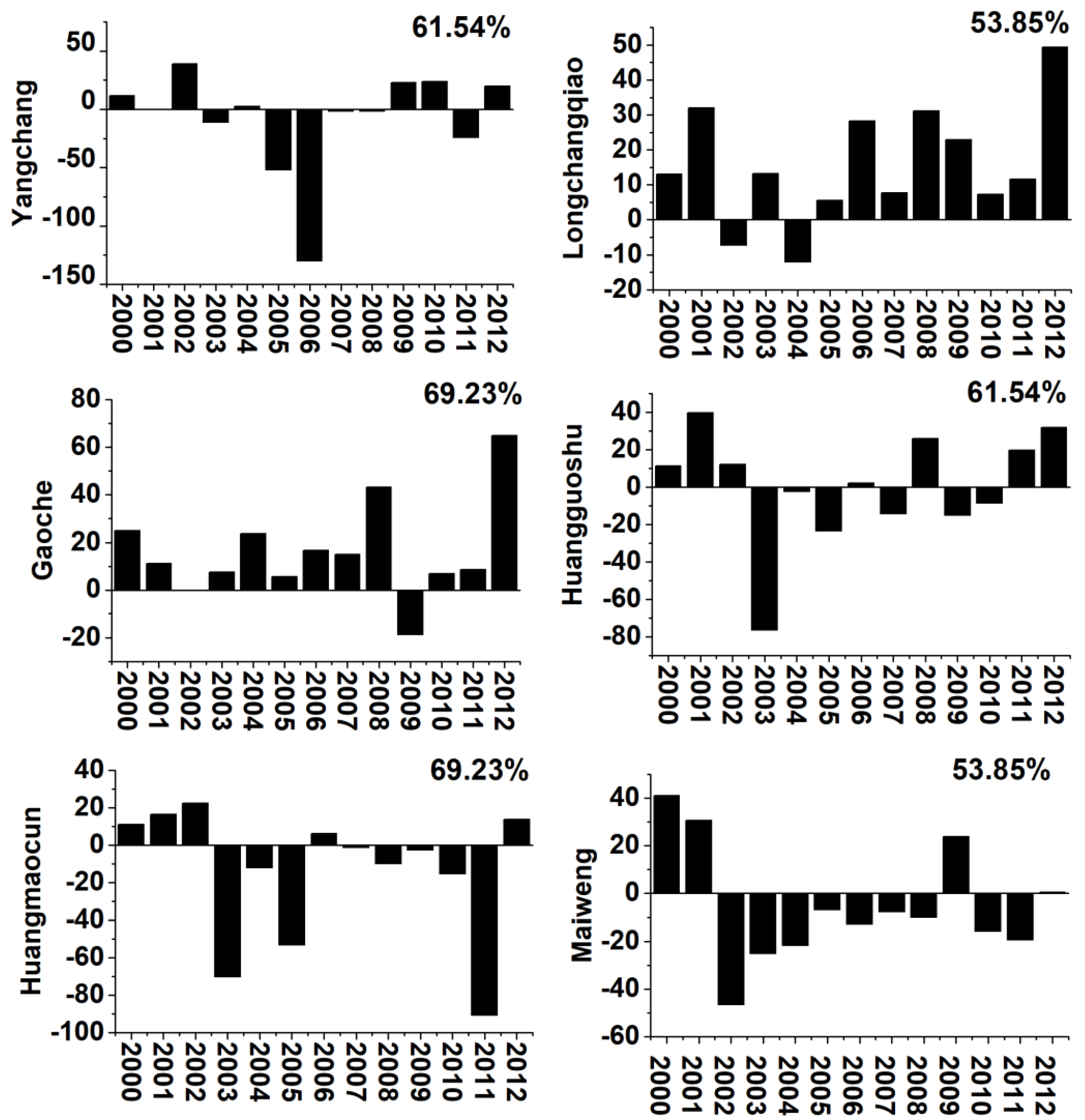
The relative errors of the main flood peaks (FPRE)in each year were calculated for the six hydrological stations. Floods within 20% of the relative error between the measured main flood peaks and the corresponding simulated flood peaks in the year were recorded as a qualified flood, and simulations of these floods had high accuracy. The ratio of the number of qualified floods to the total number of floods was the pass rate, which was calculated from 2000–2012 for each station (Figure 4).

Simulation results for the runoff of each hydrological station in Figure 3 and the results for the main-peak simulations in Figure 4 indicated that Longchangqiao and Maiweng had the worst flood peak simulations, with an FPRE of only 53.85%. For Longchangqiao, this was mainly caused by the poorly simulated flood peaks for 2005 and 2006. For Maiweng, the flood peaks for 2000 and 2002 were both underestimated and overestimated, respectively. Possible reasons for the bias in the simulation are as follows. There were two large-scale reservoirs in the small watershed of Longchangqiao, which may have had large reservoir dispatches in 2005 and 2006, giving rise to large errors in the simulated runoff. Maiweng had the smallest area among the stations, so minor regulation of reservoirs in the basin also greatly affected flood simulation peaks. Gaoche and Huangmaocun had the best main flood peak simulations, and the number of qualified floods was as high as nine. For Gaoche, the simulated flood peaks were often overestimated. For Huangmaocun, the frequencies of overestimation and underestimation of the flood peaks were similar. The flood peak simulation for the Huangguoshu station was also good. The number of qualified floods was eight, the pass rate was 61.54%, and the simulated deviations of the main flood peaks fluctuated by approximately 20% in most of the year. The number of qualified floods for the Yangchang station was also eight, but the simulation error for 2012 was close to 50%.

According to the simulation accuracy and the relative error of the flood peaks for Yangchang and Longchangqiao, which were both located on the Sancha River, we saw that if the hydrological station was farther downstream, there were more water conservancy projects in the basin, so the flow process of the section was more significantly affected. These reasons explained the phenomenon that if the hydrological station was closer to the lower reaches of the river, there were more (and larger) water conservancy projects in the river basin, and the simulation results were worse. In the Gaoche and Huangmaocun watersheds, there were few water conservancy projects, and the reservoir grade was low; thus, the error of the runoff simulation was small.

Overall, the IXAJ model did not consider the impact of water conservancy projects on the runoff in the basin; thus, the prediction of flood peaks during the flood period had different degrees of deviation. When there were many water conservancy projects in the basin, and their scales were large, the peak pass rate of the flood peaks decreased, but the simulation results were acceptable. Therefore, in a follow-up study, the influence of water conservancy projects on the runoff during flood period will be considered in the model to improve simulation accuracy.

5.2. Effect of Karst Change on Runoff

In the study area, although the karst landforms were widely distributed, the karst development degrees in different regions differed during the same period. With the change of stage, the dissolution of limestone became stronger and then weaker, and the karst fissure also changed. The enlargement of fissures led to higher flow velocities in karst fissures, and vice versa [34].

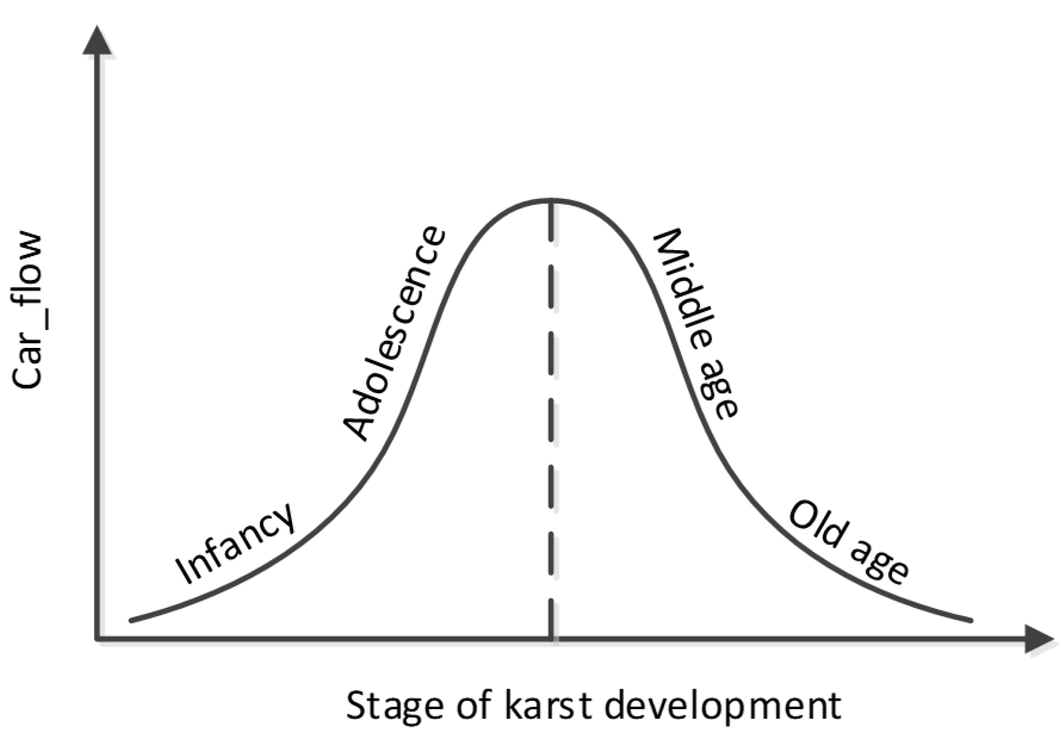
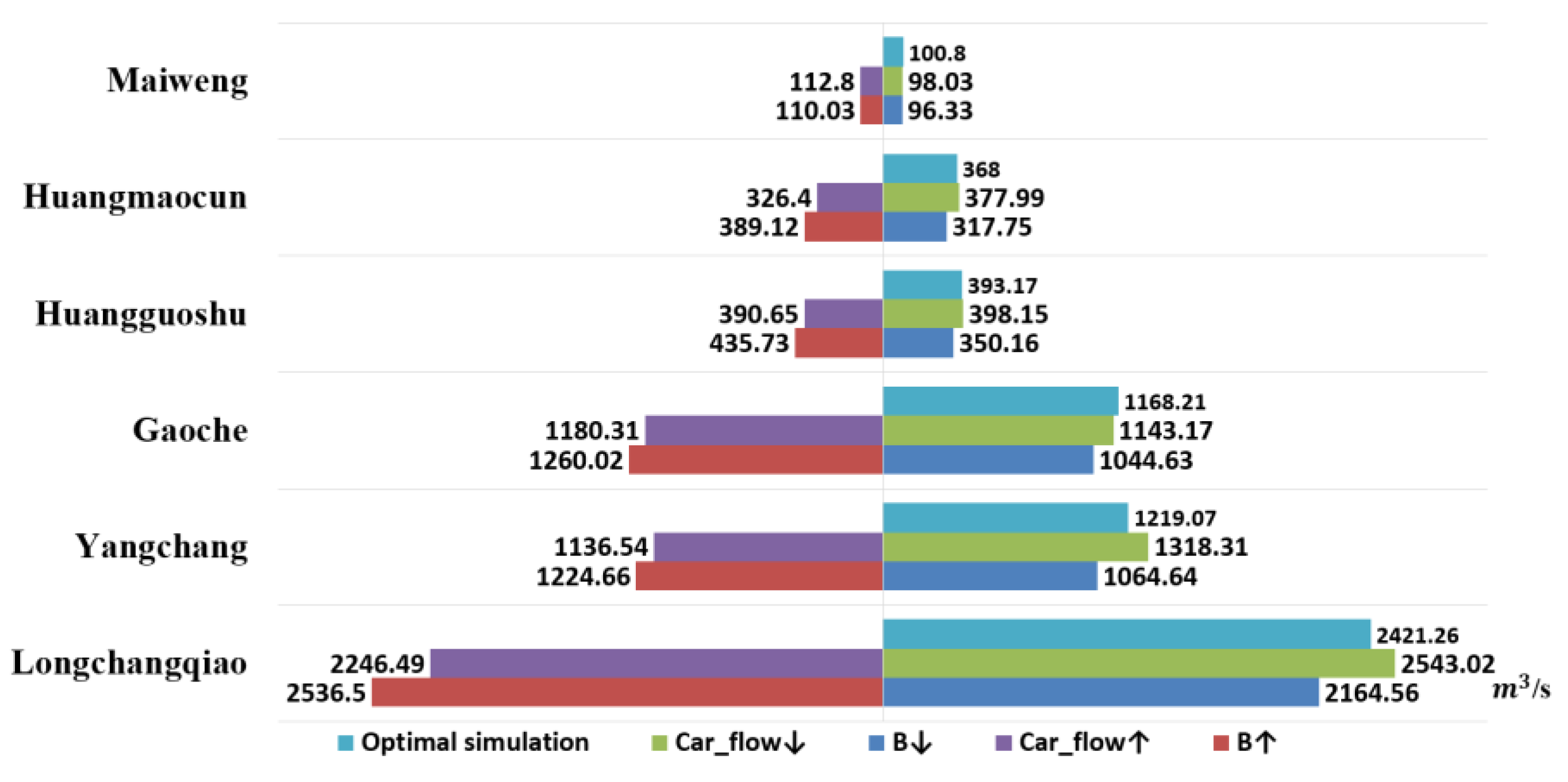
The development of the karst goes through infancy, adolescence, middle age, and finally reaching old age. This development sequence is called the stages of karst development [35]. In infancy, there are karrens, stone teeth, and dolines on the karst surface, and there is a relatively complete surface water system. The exchange of surface water and groundwater is relatively small. In adolescence, the karst surface is more developed, and there are many subterranean streams. Most of the surface water is converted into groundwater. In middle age, the surface river is blocked by lower impervious rock formation, or erosion of the surface river is stopped, the cave is further enlarged, and the cave collapses. Many subterranean streams turn into surface rivers, and many karst hills/depressions and peak forest/plains develop simultaneously. In old age, the impervious rock layers are widely exposed, and the surface water is re-exposed to form a karst plain with isolated peaks and karst hills [36]. The different stages of karst development significantly influence runoff of the basin outlet. Therefore, according to the IXAJ model, Car_flow represents the overall degree of karst development in the study area, that is, the exchange capacity of surface water and groundwater. The relationship between Car_flow and the degree of karst development can be roughly expressed by a normal distribution (Figure 5 and Figure 6), and B represents the uneven distribution of the karst development degree in the study area. On this basis, the effects of the degree of karst development and the uneven distribution of the degree of karst developments on the runoff at the outlet of the basin were simulated. However, it was impossible to know exactly at what stage each karst in the basin was in; thus, we only adjusted the change on the basis of optimal Car_flow. Because the adjustments of B and Car_flow were based on optimal simulation parameters, analysis of the change of the runoff was based on the runoff obtained via optimal parameter simulations.

This research program was divided into two types. First, the optimal parameters obtained in Section 4 were fixed, and then the runoff simulation was performed for the entire study period (2000–2012) by adjusting Car_flow or B. The specific schemes were as follows: (1) The degree of karst unevenness in the study area was constant, and the overall development degree increased and decreased. That is, B did not change, and Car_flow was adjusted to be 50% and 150% of the current optimal value. (2) The overall development degree of the karst area remained unchanged, but the degree of inhomogeneity in the area increased and decreased to 150% and 50% of the present value, respectively (0 < B < 1). In the runoff simulation of 4.2 knots, the value of B ranged from 0.15 to 0.35 because the initial karst state of the basin was unchanged. However, according to this hypothesis, the distribution of karst development changed; thus, the B range was adjusted to 0–1. The final simulation results are shown in Figure 7 and Figure 8. The value in the figures is the multiyear average daily flow.

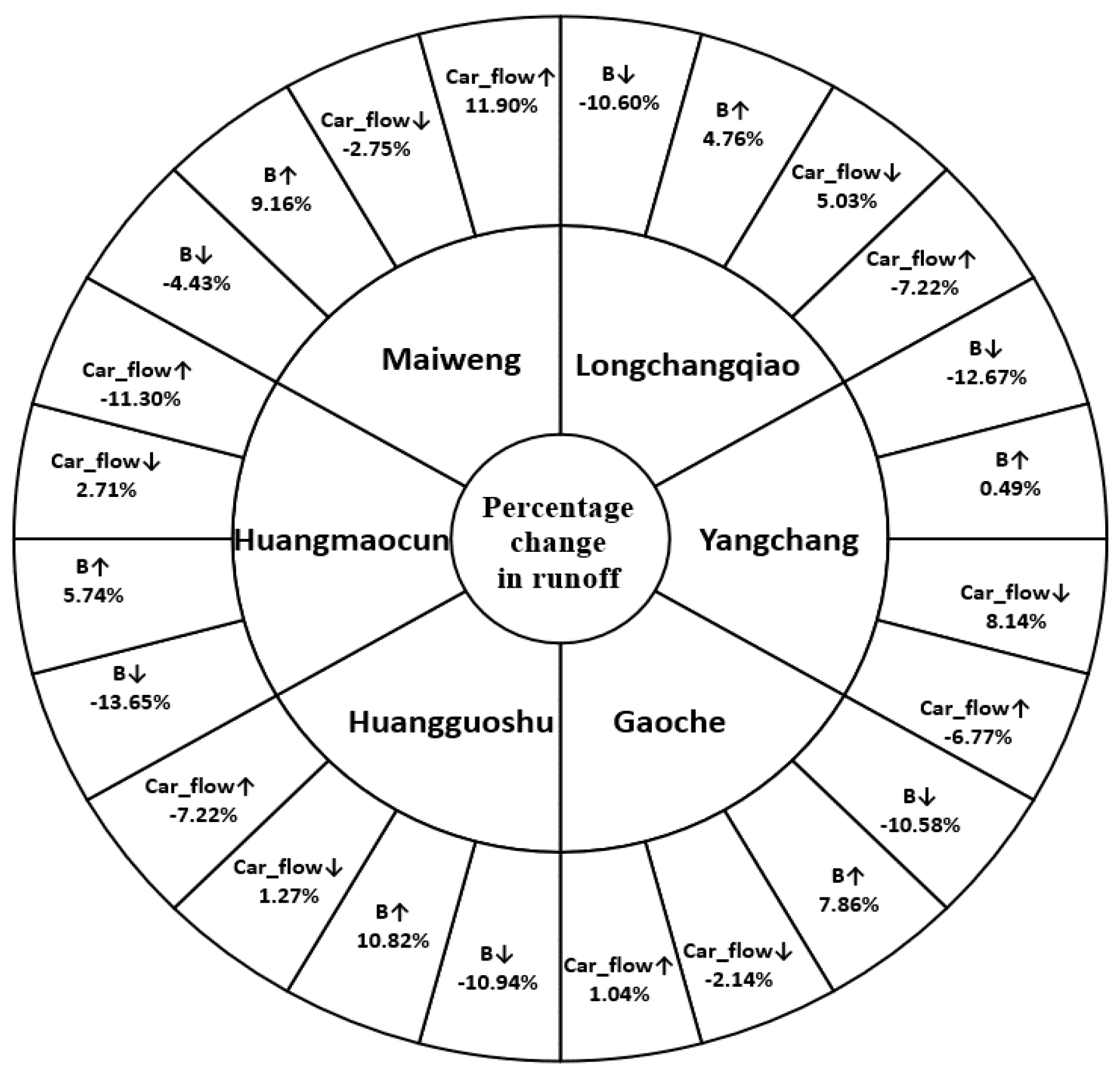
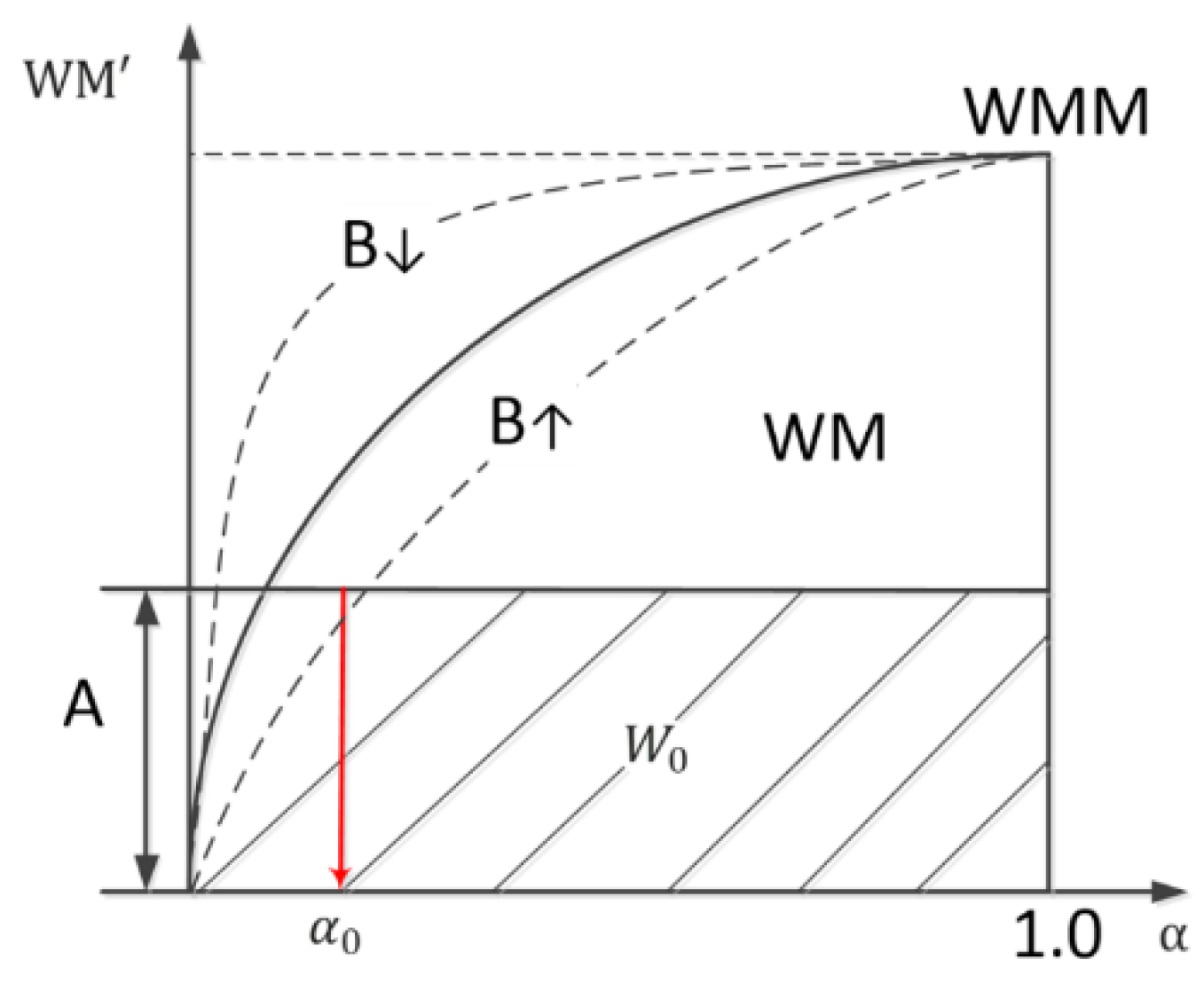
In the case of a decrease in B, the simulated runoffs for the six hydrological stations were reduced. Except Maiweng, which had the smallest basin area, the decreases of other hydrological stations were more than 10%. When B increased, all stations exhibited an increase in runoff. Therefore, in the Sancha River Basin, an increase in the uneven distribution of the karst development degree increased the runoff. If the uneven distribution of the karst development degree was reduced, the runoff of the basin outlet was reduced. In accordance with the article by the creators of the XAJ model [37], the value of B was determined by the uneven distribution of water storage conditions. Its relationship with the water storage capacity curve is shown in Figure 9, where A is the maximum field water storage capacity, and $W_0$ is the initial soil water content of the basin. The curve is expressed as $\alpha =1-{\left(1-\frac{\mathrm{WM}}{\mathrm{WMM}}\right)}^{\mathrm{B}}$. The area ${\alpha }_0$ in the basin is already full of water, and the rainfall in this area forms runoff. The rainfall in the $1-{\alpha }_0$ area cannot form runoff. Therefore, the reason karst distribution unevenness influenced variations in the runoff was as follows: on the premise that the initial soil water content in the basin was constant, a more uniform distribution of karst development yielded a smaller B and a smaller runoff generation area of the basin; thus, the runoff decreased.

When Car_flow decreased, the runoff decreased in some hydrological stations and increased in other stations. The same hydrological station could exhibit opposite changes in the runoff with both increasing and decreasing Car_flow. Among the stations, Longchangqiao, Huangmaocun, Yangchang, and Huangguoshu exhibited increased runoffs when Car_flow decreased; Maiweng and Gaoche exhibited decreased runoffs when Car_flow decreased. According to the influence of the karst on the surface runoff in different development periods, it can be estimated that the karsts of the four basins of Longchangqiao, Huangmaocun, Yangchang, and Huangguoshu were all in their youth or infancy. If Car_flow increased, the karst had a stronger development; thus, more surface water was converted into groundwater. While the karsts in the two watersheds of Maiweng and Gaoche were in middle age or old age, the increase of Car_flow degraded the karsts; thus, their ability to transform surface water into groundwater was weakened, and the runoff eventually increased.

6. Summary

The XAJ model is a conceptual model with the characteristics of high generalization capability and high precision for water cycle simulation in complex regions. It combines experience and physics in a conceptual model. It can accurately simulate the water cycle and assist in water resource management and development in the karst region. But the XAJ model is imperfect regarding the description of the physical runoff process. So, this is still a problem that needs to be promptly solved in order to develop a hydrological model with a more physical meaning.

The XAJ model had difficulty in simulating the peak runoff and runoff process in the karst area, mainly because of the hydrogeological characteristics of the karst basin. This was the root cause of all errors in the hydrological model of the karst basin. The karst basin is a typical binary 3D system, and the two water systems on the surface and underground are not closed. The pipelines and cracks significantly affect the movement of water flow. The existing groundwater storage reservoirs had large regulation and storage effects, which greatly impacted the simulation results of the models. By adding the groundwater simulation system in the karst area to the model, the actual situation of the underlying surface of the basin can be more closely reflected. In this study, according to the geological and hydrological characteristics of the karst area, a system of linear reservoirs was used to simulate the karst hydrological process, and the advantages of using linear reservoirs to simulate groundwater in the karst area were verified. Overall, the IXAJ model reduced the runoff error caused by karst fissures in the karst basin.

Finally, the effects of the degree of karst development and the unevenness of the karst spatial distribution on the runoff at the outlet of the basin were discussed. However, owing to the lack of data, the spatial and temporal distributions of the karst in the Sancha River Basin could not be specifically described. They could only be replaced by the generalization of the parameter Car_flow. Results indicated that the development degree and spatial distribution of the karst had significant effects on runoff. Therefore, accurately describing temporal and spatial distributions of the karst is crucial to accurately simulate the outlet flow of a basin.

References

- Ford, D.C.; Williams, P.W. Karst Hydrogeology and Geomorphology; John Wiley & Sons: Hoboken, NJ, USA, 2007. [Google Scholar]
- Bakalowicz, M. Karst groundwater: a challenge for new resources. Hydrogeol. J. 2005, 13, 148–160. [Google Scholar] [CrossRef]
- Bonacci, O. Karst springs hydrographs as indicators of karst aquifers. Hydrol. Sci. J. 1993, 38, 51–62. [Google Scholar] [CrossRef] [Green Version]
- White, W.B. Geomorphology and Hydrology of Karst Terrains; Oxford University Press: Oxford, UK, 1988. [Google Scholar]
- Williams, P.W. The role of the epikarst in karst and cave hydrogeology. Int. J. Speleology 2008, 37, 1–10. [Google Scholar] [CrossRef]
- Bonacci, O.; Ljubenkov, I.; Knezic, S. The water on a small karst island: the island of korcula (croatia) as an example. Environ. Earth Sci. 2012, 66, 1345–1367. [Google Scholar] [CrossRef]
- Bai, X.; Zhang, X.; Long, Y.; Liu, X.; Zhang, S. Use of 137Cs and 210Pbex Measurements on deposits in a karst depression to study the erosional response of a small karst catchment in southwest China to land-use change. Hydrol. Process 2013, 27, 822–829. [Google Scholar] [CrossRef]
- Dubois, C.; Quinif, Y.; Baele, J.; Barriquand, L.; Bini, A.; Bruxelles, L.; Dandurand, G.; Havron, C.; Kaufmann, O.; Lans, B.; et al. The process of ghost-rock karstification and its role in the formation of cave systems. Earth Sci. Rev. 2014, 131, 116–148. [Google Scholar] [CrossRef]
- Chao, C.; Bai, H.; Miao, X.; Yao, B. Movement characteristics of Karst water in a deep mining area. Min. Sci. Technol. 2009, 19, 14–18. [Google Scholar] [CrossRef]
- Wang, S.; Liu, Q.; Zhang, F. Karst rocky desertification in southwestern China: geomorphology, landuse, impact and rehabilitation. Land Degrad. Dev. 2004, 15, 115–121. [Google Scholar] [CrossRef]
- Yan, J.; Zhou, G.; Shen, W. Grey correlation analysis of the effect of vegetation status on surface runoff coefficient to forest ecosystems. Chin. J. Appl. Environ. Biol. 2000, 6, 197–200. [Google Scholar]
- Dong, H.; Zhang, J.; Zhang, B.; Zhang, R.; Zhou, X. Research on rain-runoff relationship in different landuse types on the loess area in western Shanxi province. J. Arid Land Resour. Environ. 2009, 23, 110–116. [Google Scholar]
- Chen, H.; Yang, J.; Fu, W.; He, F.; Wang, K.L. Characteristics of slope runoff and sediment yield on karst hill-slope with different land-use types in northwest guangxi. Trans. Chinese Soc. Agric. Eng. 2012, 28, 121–126. [Google Scholar]
- Parise, M.; Sammarco, M. The historical use of water resources in karst. Environ. Earth Sci. 2014, 74, 143–152. [Google Scholar] [CrossRef]
- Yurtsever, Y.; Payne, B.R. Time-Variant Linear Compartmental Model Approach to Study Flow Dynamics of a Karstic Groundwater System by the Aid of Environmental Tritium: A Case Study of South-Eastern Karst Area in Turkey. IAHS Publ. 1985, 161, 545–561. [Google Scholar]
- Ebru, E.; Wittenberg, H. Estimation of baseflow and water transfer in karst catchments in Mediterranean Turkey by nonlinear recession analysis. J. Hydrol. 2015, 530, 500–507. [Google Scholar]
- Rimmer, A.; Salingar, Y. Modelling precipitation-streamflow processes in karst basin: The case of the Jordan River sources, Israel. J. Hydrol. 2006, 331, 524–542. [Google Scholar] [CrossRef]
- Gilboa, Y.; Gal, G.; Markel, D.; Rimmer, A.; Evans, B.M.; Friedler, E. Effect of land-use change scenarios on nutrients and TSS loads. Environmen. Processes. 2015, 2, 593–607. [Google Scholar] [CrossRef]
- Jukić, D.; Denić-Jukić, V. Groundwater balance estimation in karst by using a conceptual rainfall-runoff model. J. Hydrol. 2009, 373, 302–315. [Google Scholar] [CrossRef]
- Željković, I.; Kadić, A. Groundwater balance estimation in karst by using simple conceptual rainfall-runoff model. Environ. Earth Sci. 2015, 74, 6001–6015. [Google Scholar] [CrossRef]
- Bai, Z.; Wang, G.J. Study on watershed erosion rate and its environmental effects in Guizhou karst region. J. Soil Erosion Soil Water Conserv. 1998, 4, 1–7. [Google Scholar]
- Zhang, J.; Zhuang, Y. Study and Application of Hydrological Model for Karst Catchments. J. Hohai Univ. 1988, 16, 68–80. (in Chinese). [Google Scholar]
- Cheng, G. The Xin’anjiang karst hydrological model. Water Resour. Power 1991, 9, 139–144. [Google Scholar]
- Arnold, J.G.; Srinivasan, R.; Muttiah, R.S.; Williams, J.R. Large area hydrologic modeling and assessment part I: model development 1. JAWRA J. Am. Water Resour. Assoc. 1998, 34, 73–89. [Google Scholar] [CrossRef]
- Ren, Q. Water Quantity and Evaluation Methodology Based on Modified SWAT Hydrological Modeling in Southwest Karst Area; China University of Geosciences: Wuhan, China, 2006. [Google Scholar]
- Beven, K.J. Distributed Hydrological Modelling Applications of the Topmodel Concept; (No. 551.498 D5); John Wiley and Sons: New York, NY, USA, 1997; 348p. [Google Scholar]
- Suo, L.; Wan, J.; Lu, X. Improvement and application of TOPMODEL in karst region. Carsologica Sinica. 2007, 26, 67–71. [Google Scholar]
- Shi, P.; Zhou, M.; Qu, S.; Chen, X.; Qiao, X.; Zhang, Z.; Ma, X. Testing a Conceptual Lumped Model in Karst Area, Southwest China. J. Appl. Math. 2013, 2013, 827980. [Google Scholar] [CrossRef]
- IPCC. Managing the Risks of Extreme Events and Disasters to Advance Climate Change Adaptation: A Special Report of Working Groups I and II of the Intergovernmental Panel on Climate Change; Cambridge University Press: New York, NY, USA, 2012. [Google Scholar]
- The Ministry of Water Resources of the P. R. China. Bulletin of Flood and Drought Disasters in China; The Ministry of Water Resources of the P. R. China: Beijing, China, 2012.
- Iacobellis, V.; Castorani, A.; Di Santo, A.R.; Gioia, A. Rationale for flood prediction in karst endorheic areas. J. Arid. Environ. 2015, 112, 98–108. [Google Scholar] [CrossRef] [Green Version]
- Apollonio, C.; Delle Rose, M.; Fidelibus, C.; Orlanducci, L.; Spasiano, D. Water management problems in a karst flood-prone endorheic basin. Environmen. Earth Sci. 2018, 77, 676. [Google Scholar] [CrossRef]
- Gill, M.K.; Kaheil, Y.H.; Khalil, A.; McKee, M.; Bastidas, L. Multiobjective particle swarm optimization for parameter estimation in hydrology. Water Resour. Res. 2006, 42. [Google Scholar] [CrossRef] [Green Version]
- Clemens, T.; Hückinghaus, D.; Liedl, R.; Sauter, M. Simulation of the development of karst aquifers: Role of the epikarst. Int. J. Earth Sci. 1999, 88, 157–162. [Google Scholar] [CrossRef]
- Davis, W.M. The Geographical Cycle. Geog. J. 1899, 14, 481–504. [Google Scholar] [CrossRef]
- Cvijic, J. Hydrographic Souterraine et Evolution Morphologique du Karst. Res. Trav. Inst. Geog. Aopine. 1918, 6, 375–426. [Google Scholar]
- Zhao, R.J. The Xin’anjiang model applied in China. J. Hydrol. 1992, 135, 371–381. [Google Scholar]
- Zhao R., J.; Zhuang Y., L.; Fang L., R.; Liu X., R.; Zhang Q., S. The Xin’anjiang model in Hydrological Forecasting. IAHS Publ. 1980, 129, 351–356. [Google Scholar]
Figure 1.
Geographical location of the study area.
Figure 2.
Schematic diagram of the confluence of the karst fissure groundwater system. (K1, K2, and K3 in the figure represent the regulation and storage coefficients of various linear reservoirs, respectively. A1, A2, and 1 − A2 − A3 are the ratios of large, medium, and small crack overflow to Car_flow, respectively. B1, B2, and B3 are proportions of the groundwater that pass out of the storage system from various linear reservoirs.).
Figure 3.
Runoff simulation processes in the model calibration period (2000–2008) and the validation period (2009–2012). (a) Runoff simulation in Yangchang hydrological station. (b) Runoff simulation in Longchangqiao hydrological station. (c) Runoff simulation in Maiweng hydrological station. (d) Runoff simulation in Huangmaocun hydrological station. (e) Runoff simulation in Huangguoshu hydrological station. (f) Runoff simulation in Gaoche hydrological station.
Figure 4.
Percentage of relative error of major flood peaks at various hydrological stations from 2000 to 2012 (%). The number in the upper right corner of each station’s histogram represents the pass rate based on 13 floods.
Figure 5.
Relationship between karst development degree and Car_flow. Car_flow represents the degree of karst development. With the different stages of karst development, the corresponding ordinates change from small to large and then smaller.
Figure 6.
Development pattern of karst landforms (from top left to bottom right are infancy, adolescence, middle age, and old age).
Figure 7.
Simulation results under each scheme. All simulation results are based on the IXAJ model. The light blue column represents the runoff simulation results under the optimal parameters, the green column represents the runoff simulated when the karst development is weakened, and the dark blue column represents the runoff simulated when the karst development is more uniform in the basin. The purple column represents the runoff simulated when the degree of karst development is enhanced, and the red column represents the runoff simulated when the degree of karst development is more uneven in the basin. The unit of runoff is m3/s.
Figure 8.
Percent change in runoff under each scheme. The small squares in the figure represent the percent change of runoff caused by different hydrological stations under different changes.
Figure 9.
Basin storage capacity curve. A is the maximum field water storage, and is the initial soil water content of the basin. The curve is expressed as . WM’ is the symbol for water storage capacity at a point in the basin, WMM represents the maximum reservoir capacity of the single point in the basin (in millimeters), and WM represents the average water storage capacity of the basin. The area in the basin is already full of water, and the rainfall in this area forms runoff. The rainfall in the area of cannot form runoff.