Simulation of Long-Term Soil Hydrological Conditions at Three Agricultural Experimental Field Plots Compared with Measurements

Abstract

Soil hydrological conditions influence crop growth and groundwater recharge and, thus, precise knowledge of such conditions at field scale is important for the investigation of agricultural systems. In our study, we analyzed soil hydrological conditions at three agricultural experimental field plots with sandy soils and different crop rotations using a 22-year period from 1993 to 2014 with daily volumetric soil water contents measured by the Time Domain Reflectometry with Intelligent MicroElements (TRIME)-method and pressure heads determined by automatic recording tensiometers. These measured data were compared with soil water contents and pressure heads simulated by a process-based agroecosystem model. Within this 22-year period, time spans with a better model performance and periods with a lower goodness of fit between simulations and observations were observed. The lower goodness of fit in the summer periods was attributed to inadequate calculations of root water uptake. Measurement errors of the TRIME-probes and differences between soil water contents measured by TRIME and pressure heads observed by tensiometers due to different measurement volumes, precision and measuring principles were identified as further reasons for mismatches between simulated and measured model outputs.

1. Introduction

In the field of agricultural science, soil moisture influences the germination of seeds, plant growth and plant nutrition, microbial decomposition of soil organic matter, nutrient transformations in the root zone as well as heat and water transfer at the crop-atmosphere interface [1]. In addition, the efficiency of irrigation management practices depends on an accurate in situ estimation of temporal soil moisture dynamics in the root zone. Therefore, measurement and modelling of soil moisture is important in hydrology and agriculture [2,3].

Thus, computer codes for the simulation of soil water fluxes are important parts of process-based agroecosystem models, which simulate, e.g., soil hydrology and crop growth. Such models are used to predict, e.g., the impact of different farm management practices, alternative cropping systems, climate change and drought on, e.g., runoff, erosion, evapotranspiration, seepage, soil water- and nutrient balance and crop growth [4,5,6,7]. However, simplified assumptions about the processes and parameters of soil water retention and soil water fluxes might make model predictions uncertain. Thus, for an estimation of the accuracy of the predictions of such models, a thorough validation by comparing in situ measured and calculated state variables such as soil water contents and pressure heads is important. Such a validation requires coherent, continuous long-term time series with a high temporal resolution of these measured state variables, especially if these models are used for the estimation of the impact of climate change [4,5,6,7,8,9]. Such estimates are based on input data obtained from climate change scenarios with time spans sometimes longer than 50 years [4,5,6,7,8,9].

For an automatic non-destructive measurement of soil water contents and pressure heads at field scale, the application of Time-Domain-Reflectometry (TDR) and Frequency Domain Reflectometry (FDR) as well as automatic recording tensiometers was established in the last decades [10,11,12]. Such measurement techniques can yield the required long-term observation periods with a high time resolution and, thus, can determine the wet and dry extremes of soil hydrological conditions. Accurate knowledge is required of both the wet extremes because of their important contribution to soil water flow and soil water storage, and the dry extremes in order to validate models of root water uptake. Several recent studies postulate a lack of long-term, multiple-year, continuous and quality checked measurements of soil hydrological conditions with high temporal resolution for the previous mentioned thorough validation of process-based agroecosystem models and corresponding model validation studies to check the quality and consistence of the model predictions for soil water balance over long-time periods [7,8,9,13,14,15].

Thus, the overall objective of our study was an analysis and modelling of long-term soil moisture dynamics at three agricultural experimental field plots. In this regard, the following specific objectives were addressed:

• Simulation of long-term soil moisture dynamics and thorough validation of a process-based agroecosystem model using long-term consistent and continuous time series of daily soil water contents measured by TDR and pressure heads observed by tensiometers and an analysis of model performance.
• Identification of reasons for mismatches between simulated and measured soil water contents and pressure heads with respect to seasonal effects, hydrometeorological conditions, soil hydraulic parameters, applied measurement techniques, cultivated crop types and model assumptions.

Our 22 year dataset covered several vegetation periods with different crops and a wide range of wet, dry, cool and warm years and, thus, offer new opportunities for, e.g., model parametrization, model validation, analysis of soil water extraction by vegetation cover and model comparison as compared to other recent studies using similar measurement set ups with a focus on model validation with distinct shorter time periods and with a lower variation in vegetation or crop cover [13,16,17,18,19,20,21,22,23,24].

2. Materials and Methods

2.1. Simulation Model

In our study, we used the modelling system THESEUS [25]. In THESEUS, crop growth is simulated using algorithms obtained from the Wofost7.1 model [26]. These algorithms calculate phenological development, CO₂-assimilation, root water uptake (RWU), growth and maintenance respiration, distribution of assimilates on stem, leaf, fruit and root as well as dry matter formation. Daily potential evapotranspiration ET_p (mm day⁻¹) is calculated using a modified Penman-approach [27,28] as

$${\mathrm{ET}}_{\mathrm{p}}=\frac{\Delta ·{\mathrm{R}}_{\mathrm{na}}+\mathsf{\gamma }·(0.26·\left({\mathrm{e}}_{\mathrm{s}}-{\mathrm{e}}_{\mathrm{a}}\right)·\left(\mathrm{f}+\mathrm{c}·\mathrm{u}\left(2\right)\right)}{\Delta +\mathsf{\gamma }},$$

(1)

where Δ is the slope of the saturation vapor pressure curve in kPa °C⁻¹; R_na is the net radiation defined as evapotranspiration equivalent in mm day⁻¹; γ is the psychrometer constant = 0.65 in kPa °C⁻¹; e_s is the saturated vapor pressure and e_a is the actual vapor pressure, both in kPa; f is an empirical constant = 1.0 and c is an empirical coefficient calculated from the difference between daily maximum and minimum air temperature; u(2) is the mean windspeed at 2 m height in m s⁻¹.

Soil evaporation is restricted to the soil surface layer and is limited by soil water content at air dryness. Leaf area index (LAI) is the major determinant for light absorption and photosynthesis of the crop and for partitioning of ET_p in potential soil evaporation E_pot and potential RWU T_pot according to [29].

$${\mathrm{E}}_{\mathrm{pot}}=\exp \left(-\mathrm{ext}\_\mathrm{coeff}·\mathrm{LAI}\right)·{\mathrm{ET}}_{\mathrm{p}}{\mathrm{and}\mathrm{T}}_{\mathrm{pot}}=\left[1-\exp \left(-\mathrm{ext}\_\mathrm{coeff}·\mathrm{LAI}\right)\right]·\mathrm{ETp},$$

(2)

where ext_coeff is a crop specific extinction coefficient of radiation [29]. Thus, the crop growth model simulates growth of LAI with a high level of detail. In contrast, rooting depth is simulated in a more simplified manner. After initialization, the crop grows with a fixed daily increase in rooting depth until either a crop-specific maximum depth or a soil-defined maximum depth is reached or if there is no partitioning of biomass to roots anymore. Crop growth is limited by soil water availability for RWU, temperature stress and oxygen shortage due to stagnant water in the root zone [26]. The distribution of soil water extraction by RWU between soil surface and simulated actual rooting depth L is calculated according to [30].

$$\mathrm{g}\left(\mathrm{i}\right)=\frac{\left(\mathrm{c}+1\right)·\left(\frac{\mathrm{L}·\mathrm{c}-\mathrm{x}}{\mathrm{L}·\mathrm{c}+\mathrm{x}-1}\right)·\frac{1}{\mathrm{L}}}{\left(\mathrm{c}+1\right)·\ln \left(\frac{\mathrm{c}+1}{\mathrm{c}}\right)-1},$$

(3)

where g(i) is the fraction of RWU extracted from soil layer i, x is the difference between soil surface and the soil layer i in dm and c is a parameter for the position of water extraction in the soil profile. The higher the value of c, the higher is RWU in the upper soil layers. In our study we used a value of c = 10 [30]. The impact of soil water availability on RWU at each soil layer i is calculated as:

$${\mathrm{RFWS}}_{\mathrm{i}}=\frac{{\mathsf{\theta }}_{\mathrm{a},\mathrm{i}}-{\mathsf{\theta }}_{\mathrm{wp},\mathrm{i}}}{{\mathsf{\theta }}_{\mathrm{cri},\mathrm{i}}-{\mathsf{\theta }}_{\mathrm{wp},\mathrm{i}}}{\mathsf{\theta }}_{\mathrm{cri},\mathrm{i}}=\left(1-\mathrm{p}\right)·\left({\mathsf{\theta }}_{\mathrm{fc},\mathrm{i}}-{\mathsf{\theta }}_{\mathrm{wp},\mathrm{i}}\right)+{\mathsf{\theta }}_{\mathrm{wp},\mathrm{i}}.$$

(4)

Here, RFWS_i is the dimensionless reduction factor for RWU from 0 to 1, θ_a,i is actual soil water content in soil layer i, θ_wp,i is soil water content at wilting point, θ_fc,i is soil water content at field capacity, θ_cri,i is critical soil water content defined as the threshold below which RWU is reduced. All these values are in cm³ cm⁻³. The soil water depletion fraction p is a function of ET_p and depends on the drought sensitivity of the crop. Values of the ratio actual versus potential RWU < 1 reduce gross assimilation and, thus, crop growth.

The simulation of soil water fluxes is based on a numerical solution of the flux density and continuity equations [25,31]. The flux density q in cm day⁻¹ is calculated as

$$\mathrm{q}=\mathrm{K}\left(\mathrm{h}\right)·\frac{\partial \mathrm{H}}{\partial \mathrm{z}}\mathrm{with}\mathrm{H}=\mathrm{h}+\mathrm{z},$$

(5)

where H is the hydraulic head composed of soil water pressure head h and gravitational head z, both in cm; K(h) is the soil hydraulic conductivity in cm day⁻¹ and z is the depth in cm. Changes in soil water contents per time step ∂t are obtained from the continuity equation.

$$\frac{\partial \mathsf{\theta }}{\partial \mathrm{t}}=\frac{\partial \mathrm{q}}{\partial \mathrm{z}}+\mathrm{s},$$

(6)

where s is the sink term in cm d⁻¹ and θ is the soil water content in cm³ cm⁻³. The soil water retention θ(h) and hydraulic conductivity functions K(h) were described by the equations according to [32,33].

$$\mathrm{K}\left(\mathrm{h}\right)=\frac{{\mathrm{K}}_{\mathrm{sat}}{(1-{\left(\mathsf{\alpha }\left|\mathrm{h}\right|\right)}^{\mathrm{n}-1}{\left[1+{\left(\mathsf{\alpha }\left|\mathrm{h}\right|\right)}^{\mathrm{n}}\right]}^{-\mathrm{m}})}^2}{{(1+{\left(\mathsf{\alpha }\left|\mathrm{h}\right|\right)}^{\mathrm{n}})}^{\frac{\mathrm{m}}{2}}}\mathrm{and}\mathsf{\theta }\left(\mathrm{h}\right)={\mathsf{\theta }}_{\mathrm{r}}+\frac{{\mathsf{\theta }}_{\mathrm{s}}-{\mathsf{\theta }}_{\mathrm{r}}}{{(1+{\left(\mathsf{\alpha }\left|\mathrm{h}\right|\right)}^{\mathrm{n}})}^{\mathrm{m}}},$$

(7)

where K_sat is the saturated hydraulic conductivity in cm day⁻¹; α in cm⁻¹ and n without dimensions are soil-specific parameters with the restriction m = 1− 1/n; θ_s is the saturated and θ_r is the residual soil water content. These parameters are referred to herein as vGM-parameters.

2.2. Description of the Test Site

The Experimental Station of the Leibniz Center for Agricultural Landscape Research (ZALF), Müncheberg, Germany is located around 50 km east of Berlin (52°52′ N, 14°07′ E, 62 m.a.sl.)

At three field plots (Figure A1), measurement systems were installed for long-term monitoring for soil hydrological conditions in terms of soil water contents and pressure heads under rain-fed conditions. The dataset consists of daily precipitation, global radiation, maximum and minimum air temperature, wind speed, saturation deficit of air and soil temperatures measured by an automatically recording weather station located in the Northwestern part of the field plots (Figure A1), soil profile data (

Table 1. Soil physical parameters, horizon classification according to [34].

Horizon	Depth from to (cm)	Sand (%)	Clay (%)	Silt (%)	Organic Carbon (%)	Bulk Density (g cm−3)
Plot 1
Ap	0–30	90	7	3	0.45	1.45
Ael	30–60	90	5	5	0.26	1.50
Bt	60–90	80	12	8	0.10	1.55
C1	90–120	90	4	6	-	-
C2	120–200	90	3	7	-	-
Plot 2
Ap	0–30	85	5	10	0.45	1.45
Ael	30–90	90	5	5	0.26	1.50
Bt1	90–130	80	12	8	0.10	1.55
Bt2	130–170	80	10	10	-	-
C	170–200	90	5	5	-	-
Plot 3
Ap	0–30	85	6	9	0.45	1.45
Ael	30–100	90	5	5	0.26	1.50
Bt1	100–110	81	13	7	0.10	1.55
Bt2	110–200	80	11	9	-	-

) and parameters of soil water retention curves and hydraulic conductivity functions (

Table 2. Parameters θ_s, θ_r, n and α for θ(h)-and K(h)-functions and saturated hydraulic conductivities K_sat, data from [35] (modified).

	θs (cm3 cm−3)	θr (cm3 cm−3)	n	α (cm−1)	Ksat (cm day−1)
Plot 1
Ap	0.38	0.03	2.013	0.021	92
Ael	0.32	0.03	2.179	0.027	162
Bt	0.38	0.07	2.147	0.028	30
C1, C2	0.32	0.03	2.379	0.027	162
Plot 2
Ap	0.39	0.03	2.013	0.021	92
Ael	0.32	0.03	2.179	0.027	162
Bt1, Bt2	0.39	0.07	2.147	0.028	30
C	0.32	0.03	2.379	0.027	162
Plot 3
Ap	0.39	0.03	2.013	0.021	92
Ael	0.32	0.03	2.379	0.027	162
Bt1, Bt2	0.39	0.07	2.147	0.028	30

).

The soil type is an Eutric cambisol according to the Food and Agriculture Organization FAO-classification [36]. This field experiment was established to investigate the influence of different cropping systems at each plot on crop and soil parameters and to generate datasets for agroecosystem modelling, model parametrization, model validation and model comparison. Three different farming systems with different intensity levels were investigated from 1993 to 1998 (

Table A1. Crop rotation, sowing date, harvest date and yield data (t ha⁻¹), Plot 1 ([38], modified).

Year	Crop	Sowing (day.month.year)	Harvest (day.month.year)	Observed Yield	Simulated Yield
1993	Sugar beet	26.04.93	06.10.93	8.455	9.955
1993/1994	Winter wheat	15.10.93	29.07.94	4.516	6.150
1994/1995	Winter barley	26.09.94	21.07.95	5.652	7.988
1995/1996	Winter rye	02.10.95	21.08.96	6.812	8.423
1996	Oil redish (winter catch crop)	05.09.96	-	-	-
1997	Sugar beet	03.04.97	23.09.97	11.639	10.789
1997/1998	Winter wheat	08.10.97	27.07.98	3.490	5.120
1999	Lucerne-clover-grass-mix	-	-	-	-
2000	Lucerne-clover-grass-mix	-	-	-	-
2000/2001	Winter wheat	20.09.00	27.07.01	6.678	6.695
2001/2002	Winter barley	21.09.01	06.06.02	-	-
2002/2003	Winter oilseed rape	19.08.02	11.07.03	2.780	1.988
2003/2004	Winter triticale	21.09.03	31.07.04	6.360	8.123
2004/2005	Winter rye	23.09.04	02.08.05	6.270	6.195
2006	Potatoes	24.04.06	15.08.06	4.116	3.578
2007	Sorghum	23.05.07	27.09.07	10.112	-
2008	Sorghum	29.05.08	10.09.08	5.492	-
2008/2009	Winter triticale	24.09.08	23.06.09	9.706	8.408
2009	Lucerne-clover-grass-mix	03.07.09	25.08.09	3.764	3.212
2009	“	-	20.10.09	1.155	2.112
2010	“	-	26.0510	6.421	3.762
2010	“	-	16.07.10	2.649	2.223
2010	“	-	05.10.10	4.741	3.512
2011	Lucerne-clover-grass-mix	-	21.04.11	-	-
2011	Silage maize	02.05.11	14.09.11	23.623	19.989
201/2012	Winter rye for green biomass	26.09.11	23.05.12	8.461	5.678
2012	Sorghum	24.05.12	18.09.12	10.339	-
2012/2013	Winter triticale for green biomass	28.09.12	24.06.13	10.939	8.173
2013	Lucerne-clover-grass-mix	08.07.13	10.09.13	2.564	3.121
2014	“	-	14.05.14	7.443	4.123
2014	“	-	02.07.14	5.869	3.176
2014	“	-	05.08.14	2.307	2.221
2014	“	-	09.10.14	3.561	2.456

,

Table A2. Crop rotation, sowing date, harvest date and yield (t ha⁻¹), Plot 2 ([38], modified).

Year	Crop	Sowing (day.month.year)	Harvest (day.month.year)	Observed Yield	Simulated Yield
1992/1993	Sugar beet	26.04.93	06.10.93	9.467	12.123
1993/1994	Winter wheat	15.10.93	29.07.94	3.245	5.123
1994/1995	Winter barley	26.09.94	21.07.95	3.020	4.134
1995/1996	Winter rye	02.10.95	21.08.96	2.450	4.123
1996	Yellow mustard (winter catch crop)	05.09.96	-	-	-
1997	Sugar beet	03.04.97	23.09.97	11.762	11.706
1997/1998	Winter wheat	08.10.97	27.07.98	1.430	4.123
1999	Lucerne-clover-grass-mix	-	-	-	-
2000	“	-	-	-	-
2000/2001	Winter rye	17.09.00	25.07.01	6.580	7.826
2002	Peas	11.04.02	16.07.02	2.710	-
2002/2003	Winter barley	16.09.02	14.07.03	3.600	6.720
2003/2004	Winter oilseed rape	20.08.03	23.07.04	4.280	2.315
2004/2005	Winter wheat	23.09.04	01.08.05	4.610	6.723
2006	Silage maize	02.05.06	12.09.06	5.820	6.928
2007	Winter rye for green biomass	19.09.06	24.04.07	-	-
2007	Sorghum	23.05.07	27.09.07	7.596	-
2007/2008	Winter rye for green biomass	02.10.07	28.05.08	5.710	3.935
2008	Sorghum	29.05.08	10.09.08	5.264	-
2008/2009	Winter triticale	24.09.08	23.06.09	9.365	8.322
2009	Lucerne-clover-grass-mix	03.07.09	25.08.09	4.391	3.213
2009	“	-	20.10.09	1.248	2.111
2010	“	-	26.05.10	6.374	3.517
2010	“	-	15.07.10	2.122	2.213
2010	“	-	05.10.10	5.166	3.613
2011	Lucerne-clover-grass-mix	-	21.04.11	-	-
2011	Silage maize	02.05.11	14.09.11	20.275	17.845
2011/2012	Winter rye for green biomass	26.09.11	23.05.12	6.760	3.213
2012	Sorghum	24.05.12	18.09.12	8.639
2012/2013	Winter triticale	28.09.12	24.06.13	7.248	7234
2013	Lucerne-clover-grass-mix	08.07.13	10.09.13	-	-
2014	“	-	14.05.14	5.611	3.231
2014	“	-	02.07.14	6.052	3.455
2014	“	-	05.08.14	2.712	2.221
2014	“	-	09.10.14	3.259	2.345

and

Table A3. Crop rotation, sowing date, harvest date, and yield (t ha⁻¹), Plot 3 ([38], modified).

Year	Crop	Sowing (day.month.year)	Harvest (day.month.year)	Observed Yield	Simulated Yield
1993	Sugar beet	26.04.93	06.10.93	15.427	13.896
1993/1994	Winter wheat	15.10.93	29.07.94	4.797	6.344
1994/1995	Winter barley	26.09.94	21.07.95	5.681	7.123
1995/1996	Winter rye	02.10.95	21.08.96	5.135	5.344
1996	Phacelia	05.09.96	-	-	-
1997	Sugar beet	03.04.97	23.09.97	12.419	11.762
1997/1998	Winter wheat	08.10.97	27.07.98	4.368	7.289
1999	Lucerne-clover-grass-mix	-	-	-	-
2000	“	-	-	-	-
2000/2001	Winter rye	17.09.00	25.07.01	7.965	8.242
2002	Potatoes	22.04.02	15.08.02	10.382	7.675
2002/2003	Winter wheat	20.09.02	21.07.03	4.700	6.123
2003/2004	Winter barley	14.09.03	08.07.04	6.650	8.127
2004/2005	Winter oil seed rape	20.08.04	18.07.05	3.410	1.945
2005/2006	Winter triticale	23.09.05	18.07.06	4.010	6.981
2006/2007	Winter rye for green biomass	19.09.06	21.05.07	-	-
2007	Sorghum	23.05.07	10.09.07	11.231	-
2007/2008	Winter rye for green biomass	02.10.07	30.03.08	-	-
2008	Silage maize	24.04.08	05.09.08	10.790	7.981
2008/2009	Winter rye for green biomass	24.09.08	30.03.09	-	-
2009	Silage maize	30.04.09	11.09.09	21.979	17.896
2009/2010	Winter rye for green biomass	24.09.09	30.03.10	-	-
2010	Silage maize	30.04.10	18.09.10	15.330	10.234
2010/2011	Winter rye for green biomass	24.09.10	21.04.11	-	-
2011	Silage maize	02.05.11	14.09.11	22.684	17.331
2011/2012	Winter rye for green biomass	26.09.11	11.04.12	-	-
2012	Silage maize	25.04.12	17.09.12	21.504	16.123
2012/2013	Winter rye for green biomass	28.09.12	30.03.13	-
2013	Silage maize	26.04.13	12.09.13	16.412	12.325
2014	Winter rye for green biomass	25.09.13	14.04.14	-	-
2014	Silage maize	30.04.14	18.09.14	-	-

). From 1999 to 2000, lucerne-clover-grass-mix was cultivated at all three plots to start another farming experiment (Table A1, Table A2 and Table A3). After that period, a tillage experiment was established from 2001 up to 2006 to analyze the impact of different tillage systems on yield, crop growth, soil water and matter fluxes. From 2007 up to 2014, an experiment with two different crop rotations with bio-energy crops was established to investigate the long-term influence of such rotations on soil fertility. For all three plots, crop types, sowing and harvest data, and yield data are summarized in Table A1, Table A2 and Table A3. More detailed information about this Experimental Station and the field experiments can be obtained from [37,38].

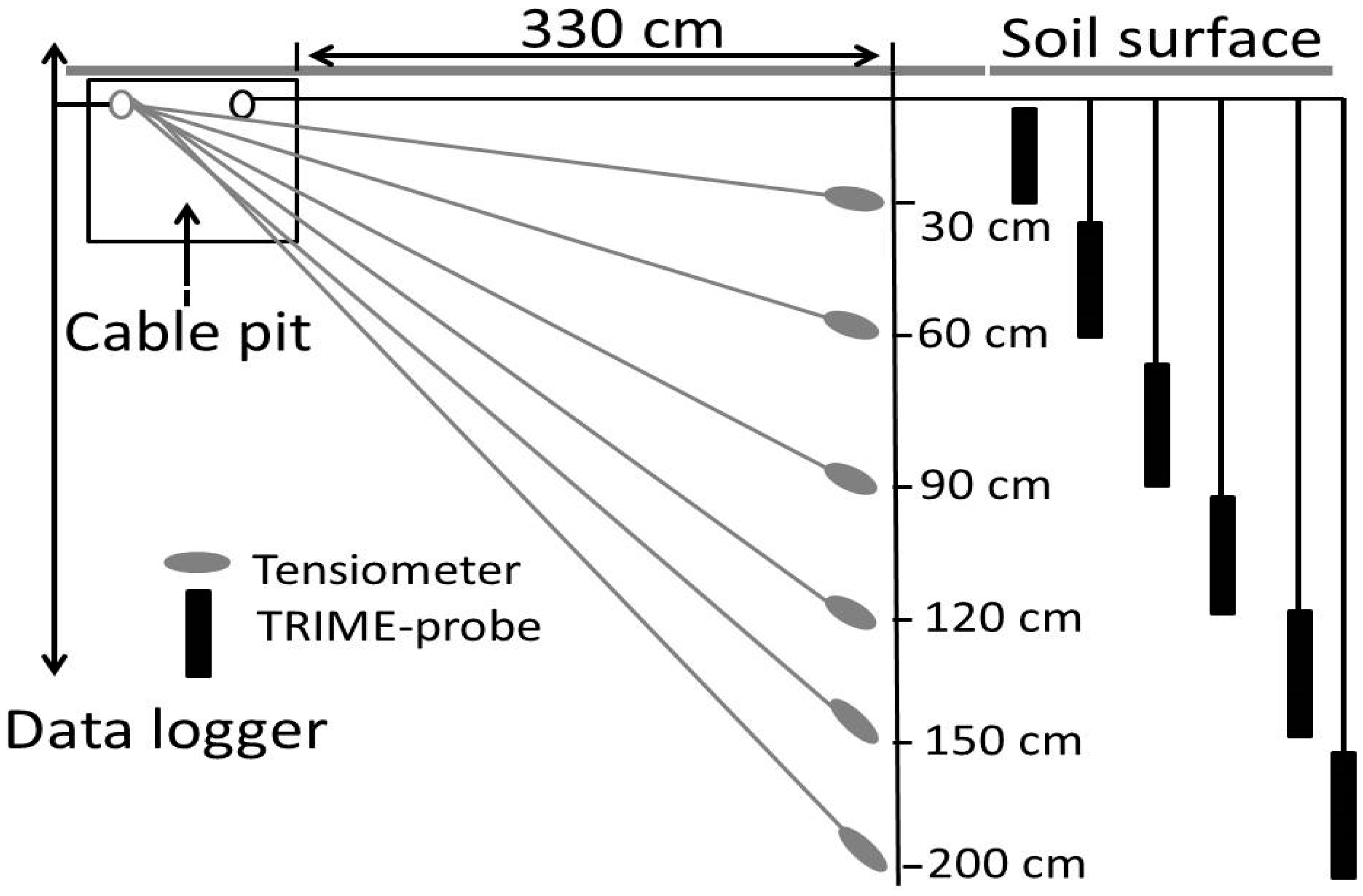
2.3. Soil Hydrological Measurements

At each of the three field plots, TRIME-(Time Domain Reflectometry with Intelligent MicroElements)-probes (Manufacturer IMKO, Germany) were installed vertically for an automatic measurement of daily volumetric depth-averaged soil water contents. The length of the probes at 26 cm (probe head: 10 cm, rod length: 16 cm) enabled the determination of soil water contents for soil compartments 0–30, 30–60, 60–90, 90–120 and 120–150 cm depth (Figure 1). This measurement setup was selected for the determination of total soil water storage in the root zone.

On each plot, soil samples were taken at 4–8 sampling times per year from the soil compartments 0–30, 30–60 and 60–90 cm depth for the determination of soil water contents using the gravimetric method in separate selected years. The measurements of the TRIME-probes were corrected using these gravimetrically determined soil water contents and the mean measurement error was estimated at ±0.025 cm³ cm⁻³ [38].

Respectively one tensiometer was installed at 30, 60, 90, 120 and 150 cm depth for the observation of daily pressure heads (Figure 1). During frost periods in the winter half years, tensiometers at 30 and 60 cm depth had to be removed to avoid frost damage. The TRIME-probes and the tensiometers were connected to a data logger. The measurements cover the time period from 1 January 1993 to 31 December 2014.

Due to the measurement setup, the TRIME-probes measure depth averaged soil water contents for a soil compartment with a thickness of app. 20–25 cm in a spherical soil volume with a diameter between 5 and 10 mm along the sensing rods of the TRIME-probes with an accuracy of ± 0.025 cm³ cm⁻³. Tensiometers determine pressure heads for a spherical soil volume with a diameter of 5–10 cm around the porous cups of the tensiometers with a precision of ±1–5 hPa [10].

The time series of observed soil water contents and pressure heads were checked by visual inspection for a detection of errors. Frozen soil conditions led to abrupt decreases of measured soil water contents because TRIME-probes detect only liquid water. These abrupt decreases ranged between 0.09 and 0.15 cm³ cm⁻³. Therefore, periods with frozen soil conditions and corresponding erroneous observed soil water contents were excluded from our analysis. After that, time series of measured soil water contents and pressure heads were checked using daily rainfall rates (precipitation→increase in soil moisture; no rainfall and evapotranspiration > 0→decrease in soil moisture). Finally, measured soil water contents and pressure heads were compared (increase of soil water contents→decrease of pressure heads; decrease of soil water contents→increase of pressure heads). Data which showed errors in both steps were flagged as erroneous and excluded from the analysis. This concerns about 15% of the measured data, and more details can be found in [38].

2.4. Estimation of Model Performance

In our study, we used the modelling efficiency index IA [39], coefficient of determination R² and the root-mean-square-deviation (RMSD).

$$\begin{array}{c}(\mathrm{a})\mathrm{IA}=1-\frac{{{\displaystyle \sum }}_{\mathrm{i}=1}^{\mathrm{n}}{\left({\mathsf{\theta }}_{\mathrm{sim}}-{\mathsf{\theta }}_{\mathrm{obs}}\right)}^2}{{{\displaystyle \sum }}_{\mathrm{i}=1}^{\mathrm{n}}{\left[\left|{\mathsf{\theta }}_{\mathrm{sim}}-{\mathsf{\theta }}_{\mathrm{obs}-\mathrm{mean}}\right|+\left|{\mathsf{\theta }}_{\mathrm{obs}}-{\mathsf{\theta }}_{\mathrm{obs}-\mathrm{mean}}\right|\right]}^2}\\ (\mathrm{b}){\mathrm{R}}^2={\left[\frac{{{\displaystyle \sum }}_{\mathrm{i}=1}^{\mathrm{n}}\left({\mathsf{\theta }}_{\mathrm{obs}}-{\mathsf{\theta }}_{\mathrm{obs}-\mathrm{mean}}\right)-\left({\mathsf{\theta }}_{\mathrm{sim}}-{\mathsf{\theta }}_{\mathrm{sim}-\mathrm{mean}}\right)}{\sqrt{{{\displaystyle \sum }}_{\mathrm{i}=1}^{\mathrm{n}}{\left({\mathsf{\theta }}_{\mathrm{obs}}-{\mathsf{\theta }}_{\mathrm{obs}-\mathrm{mean}}\right)}^2}-\sqrt{{{\displaystyle \sum }}_{\mathrm{i}=1}^{\mathrm{n}}{\left({\mathsf{\theta }}_{\mathrm{sim}}-{\mathsf{\theta }}_{\mathrm{sim}-\mathrm{mean}}\right)}^2}}\right]}^2\\ (\mathrm{c}) \mathrm{RMSD}=\sqrt{\frac{{{\displaystyle \sum }}_{\mathrm{i}=1}^{\mathrm{n}}{\left({\mathsf{\theta }}_{\mathrm{sim}}-{\mathsf{\theta }}_{\mathrm{obs}}\right)}^2}{\mathrm{n}}},\end{array}$$

(8)

where θ_sim and θ_obs are simulated and observed values; n means the number of data pairs, and θ_obs-mean and θ_im-mean are mean values. IA and R² are in a range from 0 to 1. A value of 1 suggests a perfect fit of simulated to observed values.

2.5. Model Set Up

The model calculations were carried out with a daily time step from 1 January 1993 to 31 December 2014. The soil profiles were discretized into 20 computation layers, each having a thickness of 10 cm and the downward calculated soil water flux at 200 cm depth was treated as bottom flux. The lower boundary condition for the simulation of soil water fluxes was free drainage. The initial soil water contents for the model calculations were set to soil moisture values at pressure heads of 100 hPa, which corresponds approximately to field capacity (Table 2). Simulated soil water contents of the corresponding 10 cm layers were used for the calculation of mean values of the soil compartments at 0–30, 30–60, 60–90, 90–120 and 120–150 cm depth to enable a comparison with the TRIME-measurements. For the determination of total soil water storage, simulated soil water contents of the 10 cm layers were summarized down to the lower soil profile boundary at 200 cm depth. The measured pressure heads were compared with those simulated for the corresponding computation layer.

Simulation of crop growth was initialized by seeding date and was stopped at harvest. For the parametrization of the crop growth model, we used the WOFOST parameters for Central European conditions [26]. For the crops cultivated at these three field plots (Table A1, Table A2 and Table A3), the values of ext_coeff (Equation (2)) ranged from 0.33 for winter oil seed rape up to 0.75 for potatoes [26].

3. Results

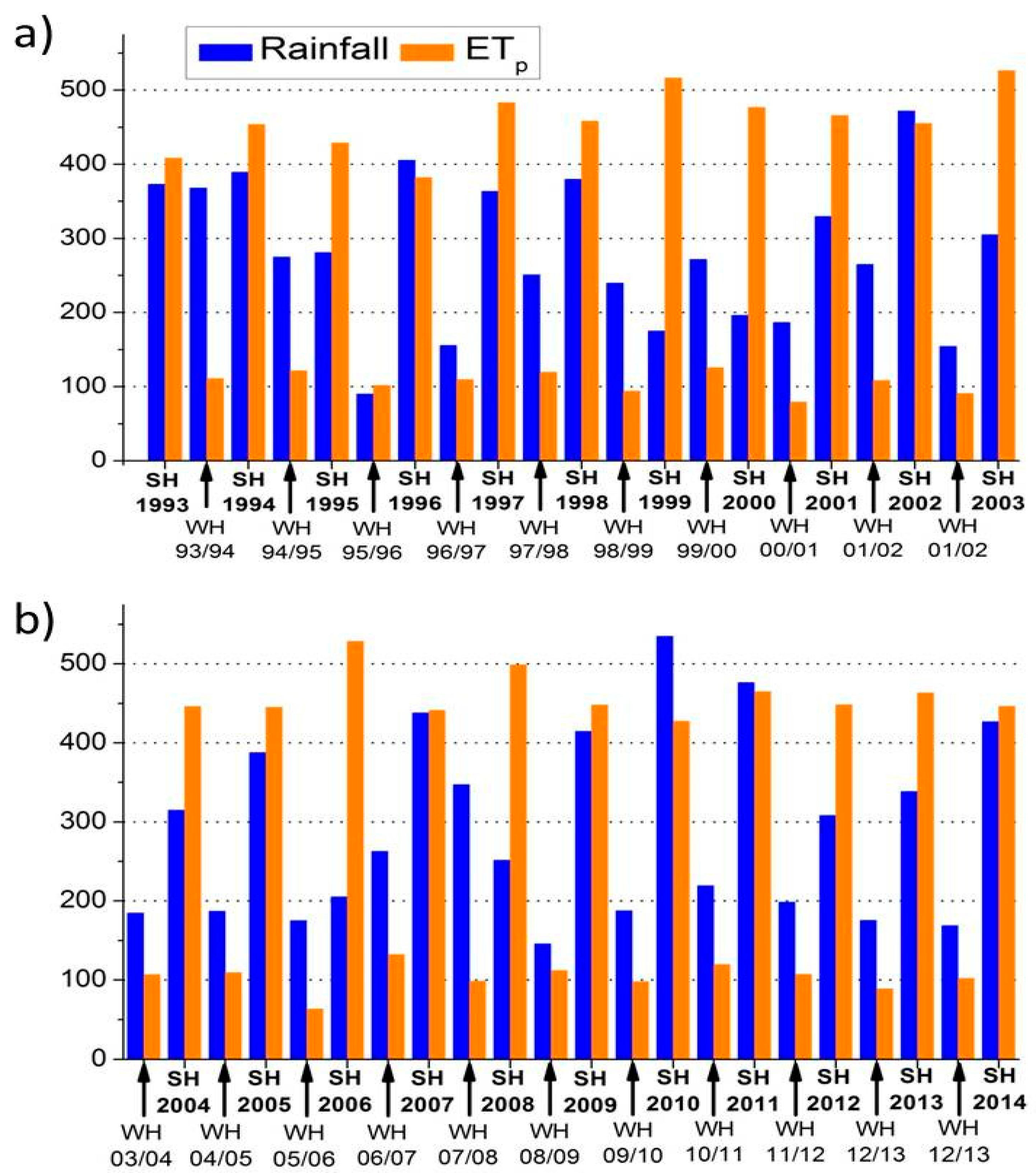
3.1. Hydrometeorological Conditions

During the 22-year period, annual rainfall ranged from 371 mm in 2006 up to 747 mm in 2002. The long-term mean annual precipitation from 1951 to 2000 is at 565 mm.

In the hydrologic winter half years (November–April), positive values of climatic water balance due to rainfall surplus were calculated (Figure 2). Only in the winter half year 1995/1996, a climatic water deficit due to rainfall at 90 mm and ET_p at 121 mm was calculated (Figure 2a).

Climatic water surplus (= rainfall > ET_p) during the hydrologic summer half years (May–October) indicated wet hydrometeorological conditions in 1996 with rainfall of 406 mm, in 2002 with 480 mm (Figure 2a), in 2010 with 535 mm and in 2011 with 476 mm (Figure 2b).

The highest climatic water deficits (= rainfall < ET_p) in the summer half years indicating dry hydrometeorological conditions were observed in 1999 with −341 mm, in 2000 with −281 mm, in 2003 with −221 mm (Figure 2a) and in 2006 with −323 mm (Figure 2b).

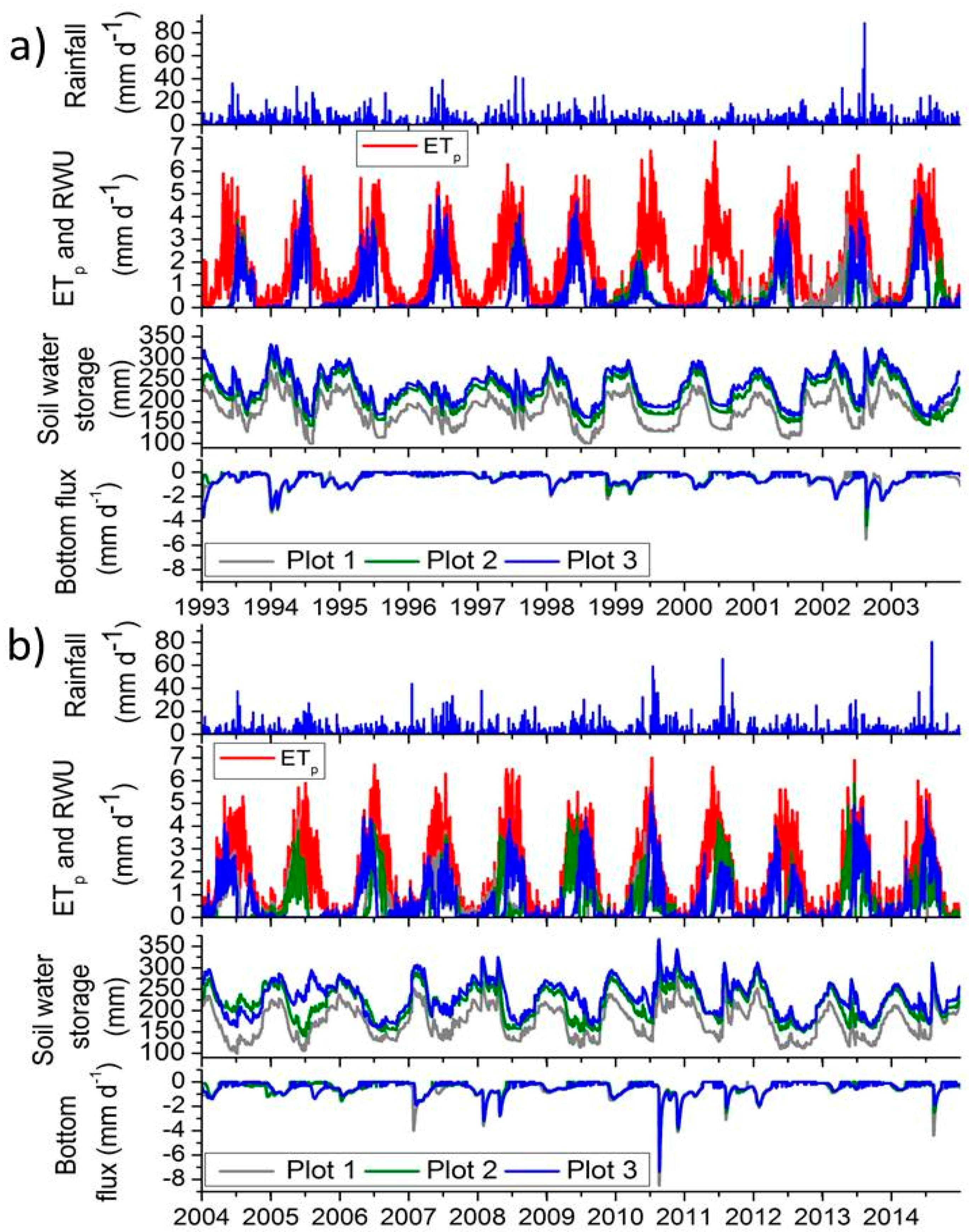
3.2. Simulated LAI, Rooting Depth, RWU, Soil Water Storage and Drainage

Since we focused on soil hydrological conditions, we compared only simulated and observed yields for a rough estimation of the plausibility of the crop growth simulations. This comparison indicated plausible calculations of crop growth (Table A1, Table A2 and Table A3). A more detailed analysis of the model performance for crop growth by comparing simulated with measured above-ground biomass at the three experimental field plots from 1993 to 1998 resulted in an IA from 0.90 to 0.99 [25].

Simulated daily values of LAI control the partitioning between RWU and soil evaporation whereas calculated rooting depth is the lower boundary of soil water withdrawal by RWU in the soil profiles (Equations (2)–(4), Figure 3). Thus, in addition to ET_p, the amount and temporal distribution of rainfall as well as soil water storage parameters, LAI and rooting depth have the highest impact on soil hydrological conditions in the summer half years. An impact of the different crop rotations on simulated RWU-rates was observed in the period from 2002 to 2012 (Figure 4). In this period, the different crops cultivated at the three plots showed higher variations in simulated LAI and rooting depth (Figure 3 and Figure 4, Table A1, Table A2 and Table A3).

The comparison of ET_p-rates with actual RWU-rates in the summer half years indicated the strong impact of the amount of soil water storage and corresponding soil water availability on RWU since RWU-rates were mainly significantly lower than ET_p, especially in the dry years 1999 and 2000 (Figure 2, Figure 3 and Figure 4). Only in wet years such as 2010, RWU-rates were closer to ET_p-rates (Figure 2, Figure 3 and Figure 4). In the winter half years, simulated daily soil water storage for the compartment 0–200 cm depth increased due to rainfall surplus and minor or no soil water withdrawal by RWU and evaporation. In the summer half years, soil water storage decreased due to soil water depletion by increased RWU and evaporation (Figure 4). However, the highest simulated soil water storage values between 297 and 364 mm were observed in the summer half years of 2002 and 2010 due to highest rainfall between 480 and 535 mm (Figure 2 and Figure 4). Simulated values of daily soil water storage at Plot 2 and Plot 3 were higher due to higher field capacity and wilting point than those calculated at Plot 1 (Figure 4,

Table 3. Porosity for 200 cm soil depth (PV_200 cm, 0 hPa), field capacity (FC_200 cm, 100 hPa), and wilting point (WP_200 cm, 15,000 hPa) calculated using vGM-data from Table 2.

	PV_200 cm (mm)	FC_200 cm (mm)	WP_200 cm (mm)
Plot 1	678	238	65
Plot 2	710	266	81
Plot 3	724	267	88

).

Longer drainage periods were calculated for the winter half years (Figure 4). However, the highest daily rainfall rates with 88 mm day⁻¹ at 12 August 2002, 59 mm day⁻¹ at 17 July 2010, 65 mm day⁻¹ at 22 July 2011 and with 80 mm day⁻¹ at 3 August 2014 resulted in the highest calculated drainage peaks from −4 to −8.8 mm day⁻¹ within the total simulation period (Figure 4). These drainage peaks at Plot 3 were lower than those calculated at Plot 1 and Plot 2 (Figure 4). This was attributed to lower K_sat at 32 cm day⁻¹ at the lower boundary of the soil profile and higher field capacity at Plot 3 as compared to K_sat-values at 162 cm day⁻¹ and lower field capacity at Plot 1 and Plot 2 (Table 2 and Table 3).

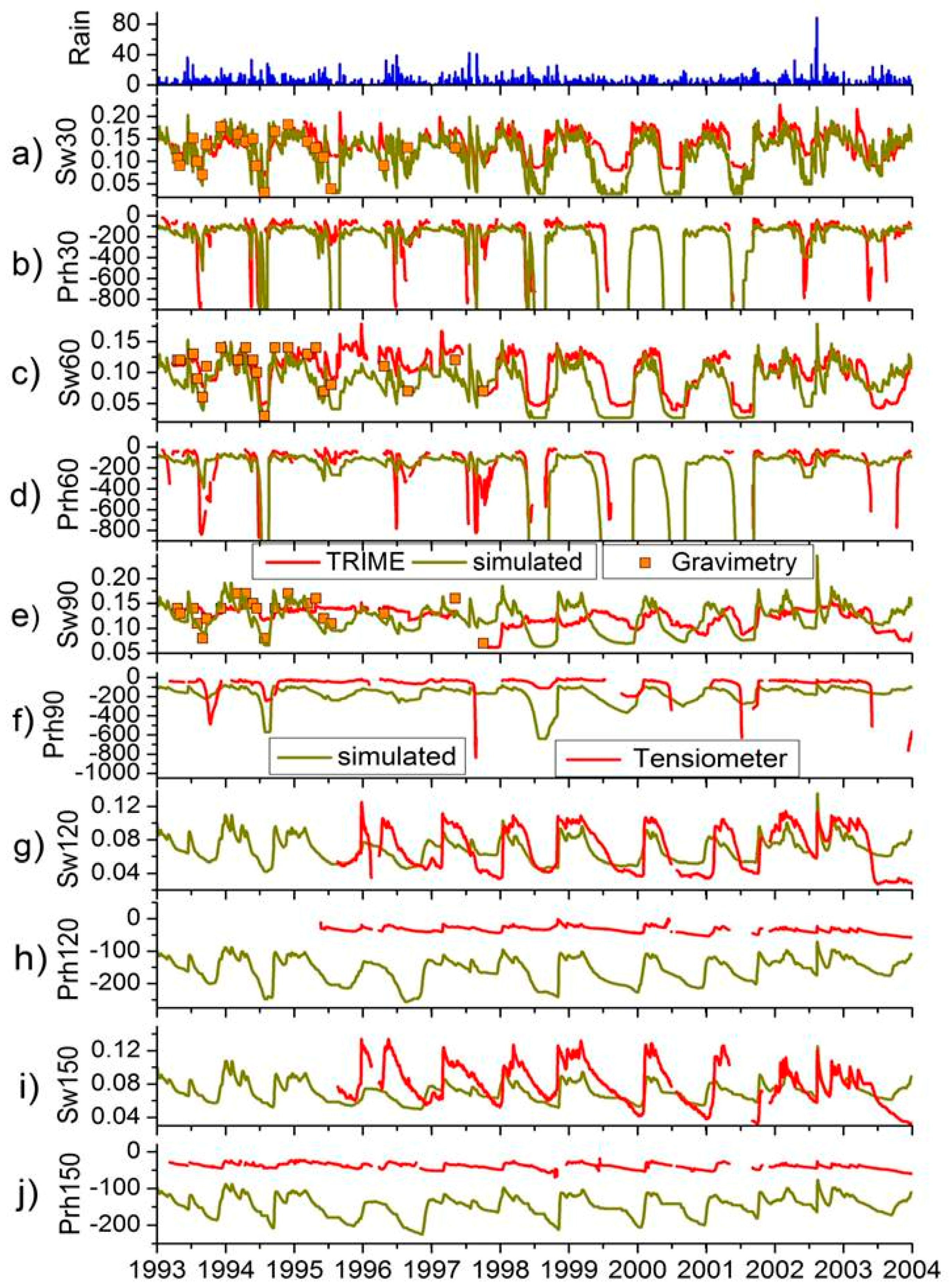
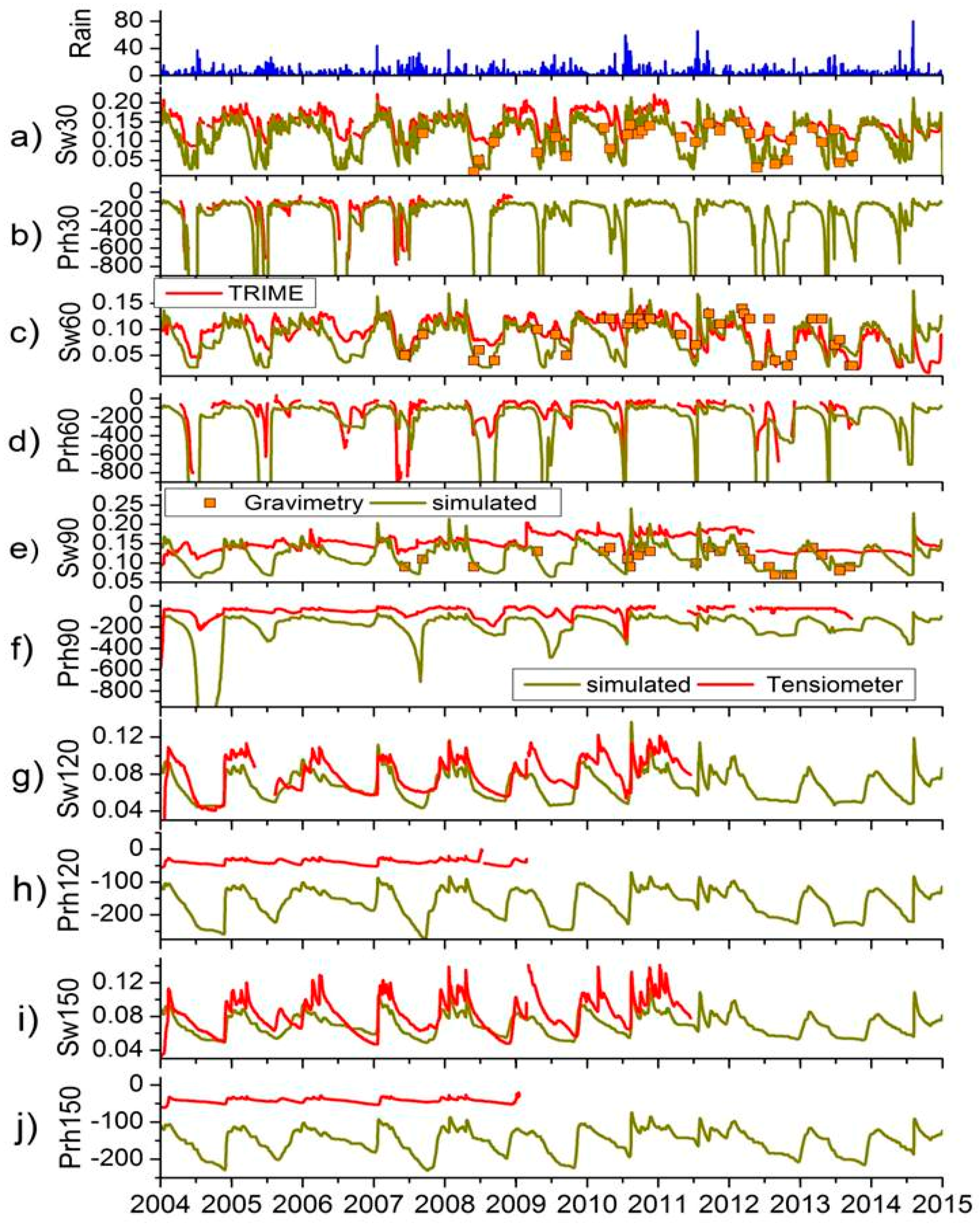
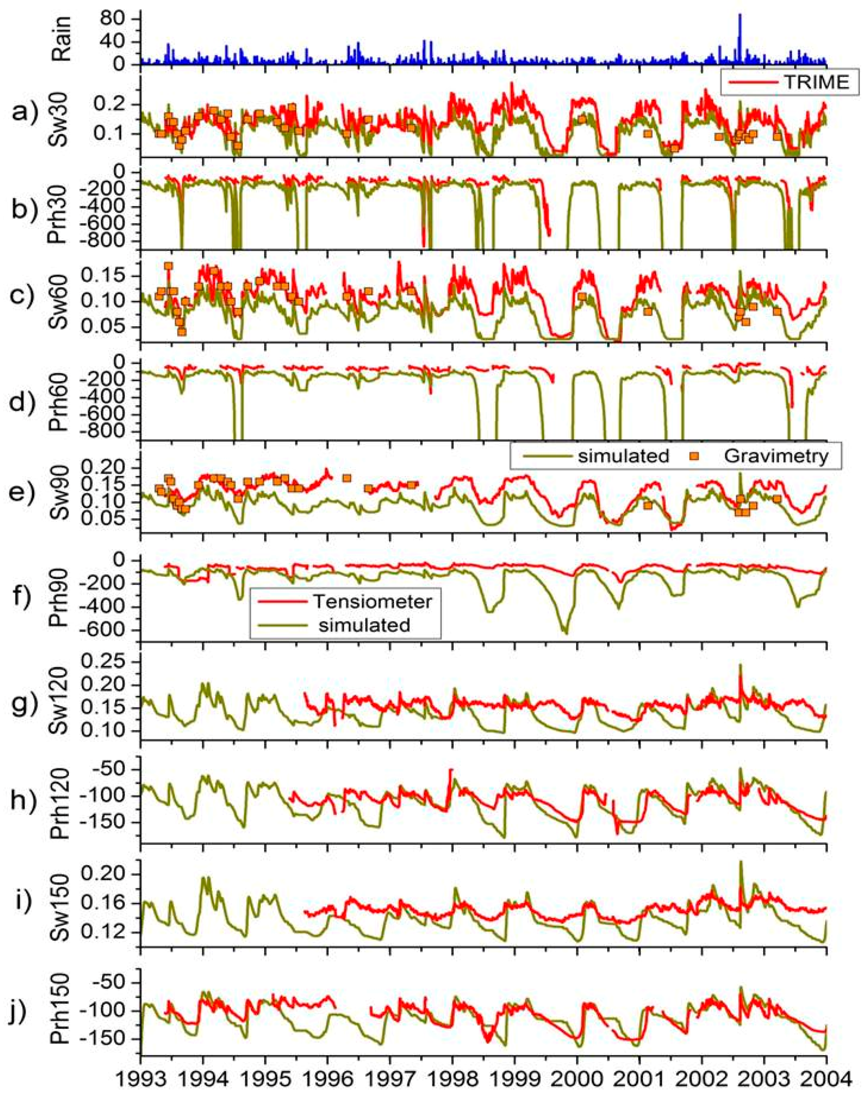
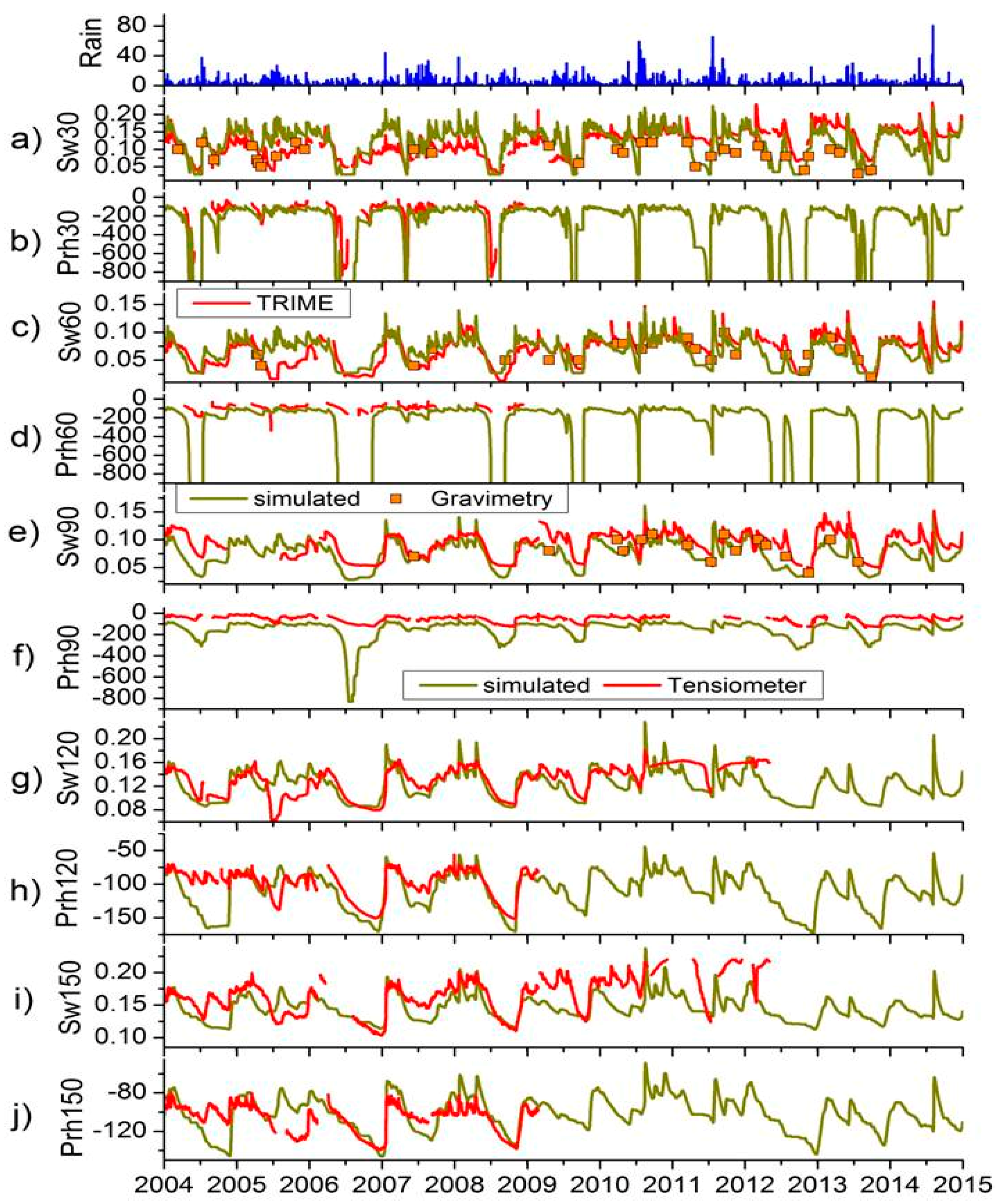
3.3. Soil Water Contents and Pressure Heads at Plot 1

Simulated soil water contents at the soil compartment 0–30 cm in the summer half years decreased to values at 0.03 cm³ cm⁻³ and were lower than those measured by TRIME with the lowest values at 0.07 cm³ cm⁻³ whereas simulated and measured soil water contents in the winter half years were in the same order of magnitude (Figure 5a and Figure 6a). Due to a sand content of 90% in this soil compartment (Table 1), a higher wilting point between 0.07 and 0.10 cm³ cm⁻³ as reason for this mismatch between simulated and measured soil water contents was estimated as unlikely [34,35]. These differences between simulated and measured soil water contents up to 0.09 cm³ cm⁻³ in the summer half years were higher than the estimated measurement error of the TRIME-probes at ±0.025 cm³ cm⁻³. This suggested higher simulated soil water extraction by RWU and evaporation as compared to the TRIME-measurements. However, simulated soil water contents in the summer half years were similar to those determined by gravimetry and calculated and measured pressure heads at 30 cm depth run mainly similar between −20 and −880 hPa as well (Figure 5a,b and Figure 6a,b). This, in turn, indicated an adequate calculation of soil water depletion by RWU and evaporation. Thus, we attributed these mismatches between simulations and observations to erroneous TRIME- measurements, particularly from 2007 to 2014 (Figure 6a). In spite of these mismatches, the model performance for soil water contents at the 0–30 cm compartment was described by an IA at 0.82, R² at 0.61 and RMSD at 0.02 cm³ cm⁻³ (

Table 4. Modelling performance for soil water contents.

Soil Compartment	Number of Data Pairs (1993–2014 = 8035 Potential Data Pairs Measured Versus Simulated Daily Soil Water Content)	IA	R2	RMSD (cm3 cm−3)
Plot 1
0–30 cm	6900	0.82	0.61	0.02
30–60 cm	7409	0.84	0.63	0.02
60–90 cm	7667	0.45	0.10	0.04
90–120 cm	5565	0.78	0.55	0.02
120–150 cm	5551	0.72	0.50	0.02
Plot 2
0–30 cm	6720	0.78	0.58	0.03
30–60 cm	6658	0.83	0.62	0.02
60–90 cm	6724	0.71	0.44	0.04
90–120 cm	5915	0.52	0.12	0.04
120–150 cm	6778	0.42	0.12	0.04
Plot 3
0–30 cm	6720	0.86	0.66	0.02
30–60 cm	7101	0.84	0.63	0.02
60–90 cm	7221	0.82	0.61	0.02
90–120 cm	5890	0.82	0.65	0.02
120–150 cm	5590	0.71	0.53	0.02

). The comparison of simulated with measured pressure heads at 30 cm depth resulted in an IA at 0.78, R² at 0.50 and RMSD at 120 hPa (

Table 5. Modelling performance for pressure heads.

Measurement Depth	Number of Data Pairs (1993–2014 = 8035 Potential Data Pairs Measured Versus Simulated Daily Pressure Head)	IA	R2	RMSD (hPa)
Plot 1
30 cm	2569	0.78	0.50	120
60 cm	3985	0.51	0.20	140
90 cm	6408	0.30	0.10	200
120 cm	4756	0.11	0.11	122
150 cm	5437	0.11	0.11	110
Plot 2
30 cm	2592	0.79	0.56	141
60 cm	2767	0.45	0.18	144
90 cm	6938	0.33	0.10	102
120 cm	5356	0.67	0.21	31
150 cm	6137	0.78	0.67	20
Plot 3
30 cm	2276	0.77	0.48	121
60 cm	2554	0.28	0.11	136
90 cm	6663	0.35	0.11	125
120 cm	4826	0.74	0.45	27
150 cm	5322	0.76	0.53	17

).

At the compartment 30–60 cm, simulated and measured soil water contents were mainly in the same order of magnitude between 0.02 and 0.18 cm³ cm⁻³ (Figure 5c and Figure 6c). Thus, IA was at 0.84, R² at 0.63 and RMSD at 0.02 cm³ cm⁻³ (Table 4). Only from 1995 to 1996, soil water contents measured by TRIME ranged above the simulated ones (Figure 5c). However, pressure heads observed at 60 cm depth declined down to values between −850 and −900 hPa in the summer half years of 1996, 1997 and 2003 whereas corresponding simulated pressure heads showed only minor decreases (Figure 5d). Therefore, IA was only at 0.51, R² at 0.20 and RMSD at 140 hPa (Table 5). This suggested an underestimation of RWU by the model in this part of the root zone for these three summer half years. However, this underestimation was confirmed by the observed soil water contents only in 2003 (Figure 5c). In this dry and hot year, measured pressure heads at 60 cm depth and soil water contents observed at the soil compartment 30–60 cm suggested higher soil water depletion by RWU as compared to the model calculations (Figure 5c,d). However, the goodness of fit between simulated soil water contents and those measured by TRIME and gravimetry in the other summer half years indicated adequate calculations of RWU by the model (Figure 5c and Figure 6c). Thus, these mismatches between measurements and simulations were attributed to erroneous TRIME-measurements in 1995 and 1996 as well as to an underestimation of RWU by the model in the summer half years of 1997 and 2003.

At the soil compartment 60–90 cm, simulated soil water contents in most of the summer half years were distinctly lower than those measured by TRIME (Figure 5e and Figure 6e). In addition, simulated pressure heads at 90 cm depth in the summer half years of 1994, 1998, 2004, 2007 and 2009 showed higher decreases than the measured ones (Figure 5f and Figure 6f). This suggested an overestimation of RWU by the model. Vice versa, soil water depletion by RWU indicated by declining measured pressure heads and low observed soil water contents in the summer half year of 2003 was not simulated adequately by the model (Figure 5e,f).

However, soil water contents determined by gravimetry in the summer half years showed a good fit to the simulated ones, particularly in 1994 and from 2007 to 2014 (Figure 5e and Figure 6e). This, in turn, indicated adequate RWU-calculations by the model. Therefore, we attributed these differences between simulated and measured soil water contents to an underestimation of RWU by the model in 2003 and to erroneous TRIME-measurements, especially from 2007 to 2014. Such erroneous measurements might be caused by soil compaction around the rods of the probes, deformations of the rods by stones during the installation, or electronic failures in the TRIME-probes, e.g., [40,41]. These mismatches between simulated and measured pressure heads and soil water contents resulted in an IA from 0.30 to 0.45, R² at 0.10 and RMSD at 0.04 cm³ cm⁻³ and at 200 hPa (Table 4 and Table 5).

At the compartments 90–120 and 120–150 cm, measured soil water contents in the winter half years ranged above the simulated ones, whereas in the summer half years observed and simulated soil water contents were mainly similar (Figure 5g,i and Figure 6g,i). The decrease of measured and simulated soil water contents down to 0.03 cm³ cm⁻³ in most of the summer half years suggested soil water withdrawal by RWU in this part of the soil profile. Only in the dry summer half year of 2003, measured soil water contents down to 0.03 cm³ cm⁻³ were lower than the simulated ones with the lowest values at 0.06 cm³ cm⁻³ (Figure 5g,i). This indicated higher RWU as compared to the model calculations. Obviously, winter oil seed rape cultivated from August 2002 to July 2003 (Figure 3a, Table A1) showed an increased RWU in these deeper soil layers to compensate soil water stress conditions in the upper soil layers. This compensation was not simulated by the model (Figure 5g,i) due to a calculated maximum rooting depth of winter oilseed rape only at 40 cm (Figure 3a). Despite these mismatches, IA ranged between 0.78 and 0.72, R² from 0.55 to 0.50 and RMSD at 0.02 cm³ cm⁻³ (Table 4).

Measured pressure heads at 120 cm and 150 cm depth between −15 and −65 hPa suggested soil water contents near or above field capacity without any soil withdrawal by RWU (Figure 5h,j and Figure 6h,j). This was in contradiction to the soil water contents between 0.03 and 0.14 cm³ cm⁻³ measured by TRIME at the soil compartments 90–120 cm and 120–150 cm (Figure 5g,i and Figure 6g,i).

These contradictions between measured soil water contents and observed pressure heads were attributed to the previous mentioned different measurement volumes, precision and measuring principles (see Section 2.3). Simulated pressure heads, however, were from −90 to −250 hPa (Figure 5h,j and Figure 6h,j). These differences led to an IA and R² at 0.11 and RMSD between 110 and 122 hPa (Table 5).

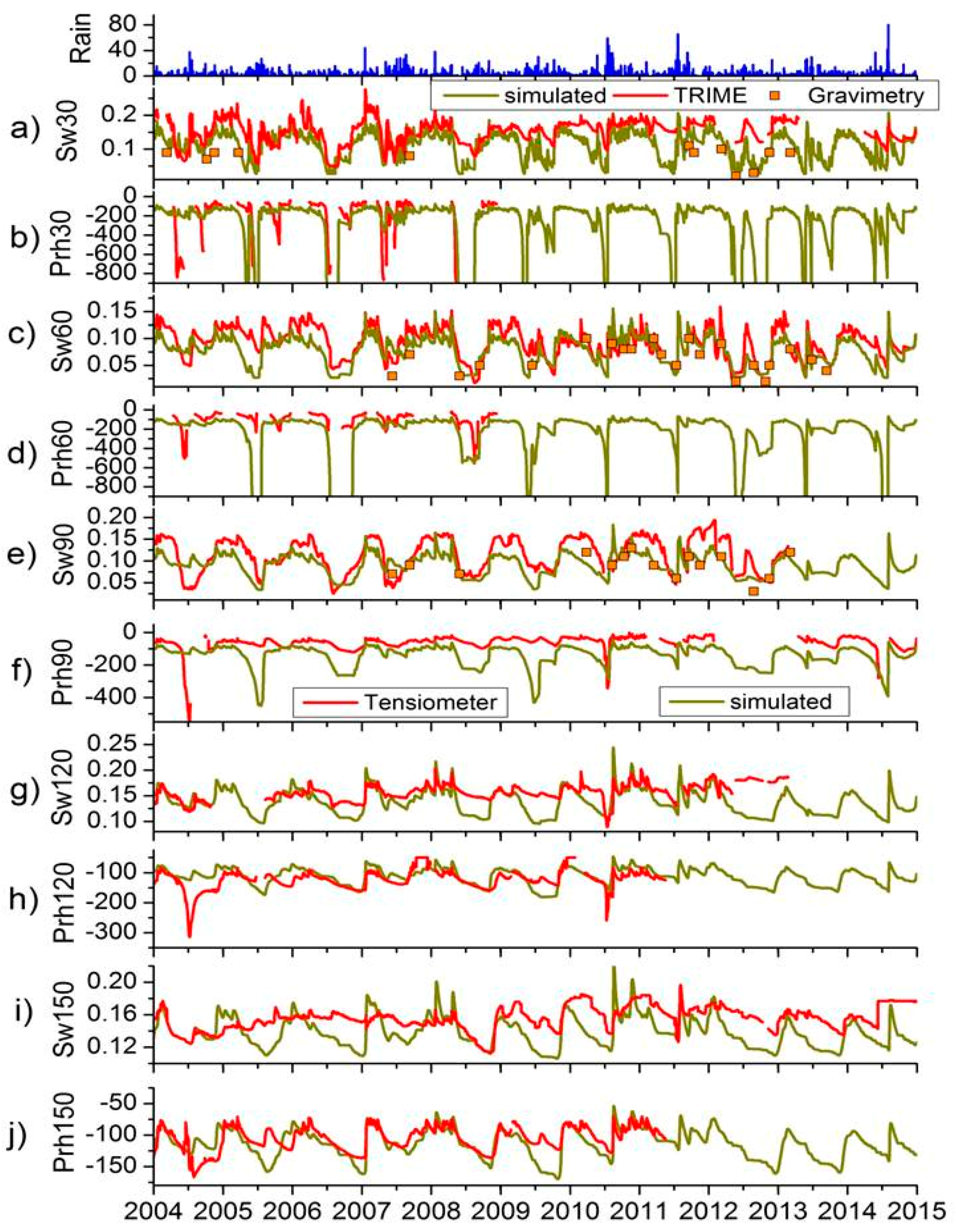
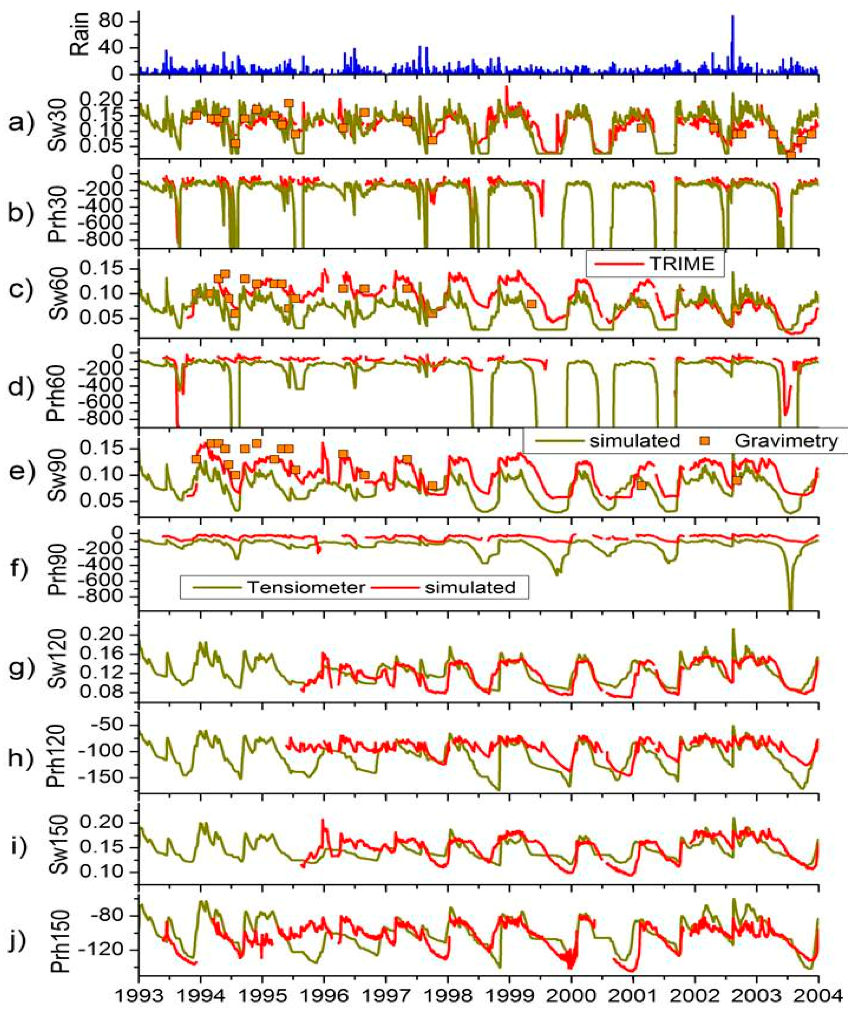
3.4. Soil Water Contents and Pressure Heads at Plot 2

Simulated soil water contents at the soil compartment 0–30 cm in the summer half years of 1994, 1995, 1996, 1998, 2002, 2003, 2005 and from 2008 to 2014 decreased to values at 0.03 cm³ cm⁻³ and were lower than the measured ones between 0.06 and 0.12 cm³ cm⁻³ (Figure 7a and Figure 8a). Despite these mismatches, IA was at 0.78, R² at 0.58 and RMSD at 0.03 cm³ cm⁻³ (Table 4). At the soil compartment 30–60 cm, simulated soil water contents in the summer half years of 1994, 1995, 1996, 1998, 2002, 2003 and 2005 down to 0.03 cm³ cm⁻³ were also lower than those measured by TRIME between 0.06 and 0.10 cm³ cm⁻³ (Figure 7c and Figure 8c). In contrast to the soil compartment 0–30 cm, simulated and measured soil water contents at the 30–60 cm soil compartment showed a good match from 2008 to 2014 (Figure 8c). Thus, IA was at 0.83, R² at 0.62 and RMSD was at 0.02 cm³ cm⁻³ (Table 4).

In addition, measured pressure heads at 30 and 60 cm depth in these summer half years showed lower decreases as compared to the simulated ones with distinct higher declines (Figure 7b,d and Figure 8b,d). This suggested an overestimation of soil withdrawal by evaporation and RWU by the model for these upper two soil compartments. This can be caused by

• Inadequate description of the spatial distribution of RWU in the root zone depending on crop specific maximum rooting depth and root density distribution.
• Overestimation of potential RWU by the model.

Potential RWU is determined by the amount of calculated ET_p and actual LAI, which depends on the current phenological development stage of the crop.

Due to higher simulated soil water withdrawal in these summer half years, calculated soil water contents up to 0.20 cm³ cm⁻³ in the consecutive winter half years such as 1994/1995, 1995/1996 and 1998/1999 were lower than the measured ones with values up to 0.26 cm³ cm⁻³ (Figure 7a,c). From 1999 to 2002 and from 2006 to 2007, simulated and measured soil water contents showed mostly a good fit for both soil compartments (Figure 7a,c and Figure 8a,c).

However, since soil water contents measured by gravimetry at the 0–30 cm compartment showed a good fit to the simulated ones in the summer half years, particularly from 2008 to 2014 (Figure 8a), we attributed these mismatches between simulated and measured soil water contents to erroneous TRIME-measurements in this period. Despite the previous mentioned differences between simulated and measured pressure heads in some summer half years, calculated and observed pressure heads at 30 cm depth showed a sufficient match suggested by an IA at 0.79, R² at 0.56 and RMSD at 141 hPa, whereas the comparison of simulated with measured pressure heads at 60 cm depth resulted in an IA at 0.45, R² at 0.18 and RMSD at 144 hPa (Figure 7b,d and Figure 8b,d, Table 5).

At the soil compartment 60–90 cm, soil water contents measured by TRIME and gravimetry were up to 0.08 cm³ cm⁻³ higher than the simulated ones from 1994 to 1999 (Figure 7e). In the remaining period from 2000 to 2014, simulated and measured soil water contents showed a better match, especially in the summer half years from 2001 to 2010. However, measured soil water contents in the winter half years were still higher than the simulated ones (Figure 7e and Figure 8e). Thus, the model performance for soil water contents was described by an IA at 0.71, R² at 0.44 and RMSD at 0.04 cm³ cm⁻³ (Table 4).

Simulated pressure heads at 90 cm depth ranged between −75 and −650 hPa whereas measured pressure heads were from −10 to −120 hPa (Figure 7f and Figure 8f). Therefore, the model performance was low with an IA at 0.33, R² at 0.10 and RMSD at 102 hPa (Table 5). This range of measured pressure heads suggested soil water contents near or above field capacity for the total investigation period. Therefore, the soil water contents at the compartment 60–90 cm measured by TRIME between 0.02 and 0.19 cm³ cm⁻³ were in contradiction to the observed pressure heads. Due to these contradictions, an identification of a reason for the mismatch between simulated and observed soil water contents from 1994 to 1999 and in the winter half years was hampered. Similar to Plot 1, these contradictions between measured soil water contents and observed pressure heads were attributed to the previous mentioned technical differences between TRIME-probes and tensiometers (see Section 2.3).

At the soil compartments 90–120 and 120–150 cm, simulated soil water contents in most of the summer half years decreased to values down to 0.10 cm³ cm⁻³ whereas corresponding measured soil water contents declined only to values between 0.13 and 0.15 cm³ cm⁻³ (Figure 7g,i and Figure 8g,i). This resulted in an IA from 0.42 to 0.52, R² at 0.12 and RMSD at 0.04 cm³ cm⁻³ (Table 4) and suggested higher simulated soil water withdrawal by RWU in this lower part of the soil profile as compared to the observations. This calculated soil water withdrawal was due to simulated maximum rooting depths of the crops at 120 cm depth in these summer half years (Figure 3). Simulated and measured pressure heads at 120 and 150 cm depth were in the same range from −50 to −180 hPa (Figure 7 and Figure 8). This resulted in an IA from 0.67 to 0.78, R² between 0.21 and 0.67 and RMSD from 20 to 31 hPa (Table 5). Despite the sufficient fit between simulated and measured pressure heads, we finally attributed the mismatches between simulated and observed soil water contents to an overestimation of RWU by the model in the summer half years in this part of the soil profile from 90 to 150 cm depth.

3.5. Soil Water Contents and Pressure Heads at Plot 3

At the soil compartment 0–30 cm, simulated soil water contents and those measured by TRIME and gravimetry showed a good fit from 1996 to 2009 (Figure 9a and Figure 10a). However, from 1993 to 1995 and from 2010 to 2014, soil water contents measured by TRIME in the summer half years decreased to values at 0.07 cm³ cm⁻³ whereas simulated soil water contents declined to lower values at 0.03 cm³ cm⁻³ (Figure 9a and Figure 10a). This indicated higher simulated soil water extraction by RWU and evaporation in the summer half years of these two periods as compared to the measurements, especially in 1995, 2011 and 2012 (Figure 9a and Figure 10a). In contrast to that, the good fit of simulated soil water contents at the 0–30 cm soil compartment to those determined by gravimetry suggested an adequate calculation of RWU by the model, particularly from 2009 to 2014 (Figure 10a). Thus, we attributed these discrepancies between observations and simulations from 1993 to 1995 and from 2010 to 2014 to erroneous TRIME-measurements (Figure 9a and Figure 10a). Despite these mismatches, IA for soil water contents was at 0.86, R² at 0.66 and RMSD at 0.02 cm³ cm⁻³ (Table 4). Measured and simulated pressure heads at 30 cm depth in the summer half years were mainly in the same order of magnitude (Figure 10b). Thus, IA was at 0.77, R² at 0.48 and RMSD at 121 hPa (Table 5).

From 1993 to 1999, soil water contents at the soil compartment 30–60 cm depth measured by TRIME and gravimetry were higher than the simulated ones (Figure 9c). In the following period from 2000 to 2014, observed and simulated soil water contents showed a distinct better match.

Therefore, IA was at 0.84, R² at 0.63 and RMSD at 0.02 cm³ cm⁻³ (Figure 9c and Figure 10c, Table 4). Measured pressure heads at 60 cm depth showed no decreases suggesting no or only minor soil water depletion whereas simulated declining pressure heads indicated higher soil water withdrawal by RWU (Figure 9d and Figure 10d). Due to these differences, IA was at 0.28, R² at 0.11 and RMSD at 136 hPa (Table 5). However, an explicit identification of reasons for this mismatch between measurements and simulations from 1993 to 1999 such as an overestimation of RWU by the model or erroneous TRIME-measurements was hampered since the time course of corresponding pressure heads measured at 60 cm depth showed a high amount of missing data (Figure 9d and Figure 10d, Table 5).

From 1993 to 2000, measured soil water contents at the soil compartment 60–90 cm were higher than the simulated ones, similar to the soil compartment 30–60 cm (Figure 9c,e). In the summer half years of 2003, 2004 and 2006, simulated soil water contents decreased to values at 0.03 cm³ cm⁻³, which were lower than those measured by TRIME with the lowest values at 0.07 cm³ cm⁻³ (Figure 9e and Figure 10e). This indicated higher simulated soil withdrawal by RWU as compared to the TRIME- measurements. However, from 2007 to 2014, simulated soil water contents and those measured by TRIME and gravimetry were mainly in the same order of magnitude (Figure 9e and Figure 10e). Therefore, IA was at 0.82, R² at 0.61 and RMSD at 0.02 cm³ cm⁻³ (Table 4). Furthermore, measured pressure heads at 90 cm depth showed only minor decreases in these summer half years as compared to the simulated ones with distinct higher declines, particularly in the dry years 2003 and 2006 (Figure 9f and Figure 10f). Thus, IA was at 0.35, R² at 0.11 and RMSD at 125 hPa (Table 5). Therefore, we attributed the differences between observations and simulations from 1993 to 2000 to erroneous TRIME-measurements and the discrepancies between simulated and measured soil water contents and pressure heads in the summer half years of 2003 and 2006 to an overestimation of RWU by the model.

Measured soil water contents at the soil compartment 90–120 cm in the summer half years 1997, 2000 and 2005 decreased to values at 0.07 cm³ cm⁻³, which were lower than the simulated ones with the lowest values at 0.09 cm³ cm⁻³ (Figure 9g). This suggested higher soil withdrawal by RWU in these summer half years as compared to the model calculations. In the other years, simulated soil and measured water contents were in the same order of magnitude (Figure 9g and Figure 10g). Thus, the model performance was described by an IA at 0.82, R² at 0.65 and RMSD at 0.02 cm³ cm⁻³ (Table 4). Simulated pressure heads at 120 cm depth ranged below the measured ones only in the summer half years of 1998, 2003 and 2004. In the other years, simulated and measured pressure heads were similar (Figure 10h). Therefore, IA was at 0.74, R² at 0.45 and RMSD at 27 hPa (Table 5).

Simulated and measured soil water contents at the soil compartment 120–150 cm were mainly similar (Figure 9i and Figure 10i). Only in the summer half years of 1997, 1999, 2000 and 2007, measured soil water contents were lower than the simulated ones, but the differences between simulated and observed soil water contents, were below the measurement error of the TRIME-probes at ±0.025 cm³ cm⁻³. Thus, IA was at 0.71, R² at 0.53 and RMSD at 0.02 cm³ cm⁻³ (Table 4). Calculated and observed pressure heads at 150 cm depth were also similar and, therefore, IA was at 0.76, R² at 0.52 and RMSD at 17 hPa (Table 5).

4. Discussion

Temporal simulated and measured soil water dynamics at all three plots were similar with increasing soil water storage during the winter half years due to rainfall surplus and decreasing soil water storage due to soil water withdrawal by evaporation and RWU in the summer half years (Figure 4, Figure 5, Figure 6, Figure 7, Figure 8, Figure 9 and Figure 10). Differences in simulated drainage and soil water storage between the three experimental field plots (Figure 4) were attributed to the different depths of the soil horizons (Table 1), which caused differences in soil water storage parameters and hydraulic conductivity, particularly at the lower boundary of the soil profiles at 200 cm depth (Table 2 and Table 3).

A distinct impact of the different crop rotations established at the three field plots on simulated soil water contents and pressure heads was observed in 2003, 2004, 2005 and 2009 (Figure 4, Figure 5, Figure 6, Figure 7, Figure 8, Figure 9 and Figure 10, Table A1, Table A2 and Table A3). In 2003, winter soil seed rape showed a simulated maximum rooting depth of 40 cm at Plot 1 in contrast to winter barley at Plot 2 and winter wheat at Plot 3 with simulated maximum rooting depths between 90 and 110 cm (Figure 3a, Table A1, Table A2 and Table A3). In 2004, winter triticale at Plot 1 and winter barley at Plot 3 showed simulated maximum rooting depths from 120 to 90 cm whereas winter oil seed rape at Plot 2 showed a simulated maximum rooting depth at 45 cm. In 2005, the crop growth model simulated rooting depths between 90 and 120 cm for winter rye at Plot 1 and winter wheat at Plot 2 in contrast to Plot 3 again with winter oil seed rape with a calculated rooting depth at 45 cm. In 2009, lucerne-grass-cover at Plot 1 and 2 showed longer vegetation periods as compared to silage maize at Plot 3 (Figure 3b). This resulted in different amounts of calculated soil water withdrawal by RWU and, thus, to different simulated soil water contents and pressure heads from soil surface down to 120 cm depth in the summer half years (Figure 4, Figure 5, Figure 6, Figure 7, Figure 8, Figure 9 and Figure 10). However, these simulated differences between the experimental field plots were only partly confirmed by the measurements.

The model performance for soil water contents in terms of IA ranged between 0.45 and 0.86, R² was from 0.10 to 0.66 and RMSD between 0.02 and 0.04 cm³ cm⁻³ (Table 4). At all three field plots, the best model performance for soil water contents was observed for the upper two soil compartments 0–30 and 30–60 cm with IA from 0.78 to 0.86, R² between 0.58 and 0.66 and RMSD at 0.02 cm³ cm⁻³ (Table 4). In other agricultural experimental field studies, the comparison of simulated soil water contents with those measured by TDR resulted in IA-values between 0.34 and 0.96 and R² from 0.27 to 0.91, e.g., [16,17,18,19,20,21,22,23,24]. The model performance for pressure heads in terms of IA ranged from 0.11 up to 0.80, R² was from 0.10 to 0.56 and RMSD between 17 and 200 hPa (Table 5). At all three plots, the best match between simulated and observed pressure heads was observed at 30 cm depth with IA from 0.77 to 0.79, R² between 0.48 and 0.56 and RMSD from 17 to 200 hPa (Table 5). In other studies, IA for pressure heads was between 0.54 and 0.93, e.g., [18].

Large differences in the model performance for soil water pressure heads at 120 and 150 cm depth were observed between Plot 1 with an IA at 0.11 and Plot 2 and 3 with IA-values between 0.67 and 0.78 (Table 5, Figure 5, Figure 6, Figure 7, Figure 8, Figure 9 and Figure 10). At Plot 1, tensiometers installed at 120 cm and 150 cm depth are located in the C-horizon with a sand content at 90%. At Plot 2 and 3, corresponding tensiometers are located in the Bt-Horizons with sand contents at 80% (Figure 1, Table 1). These differences between Plot 1 and Plots 2 and 3 regarding soil texture led to different vGM-parameter sets in this lower part of the soil profile with an impact on simulated soil water storage and drainage (Figure 4). However, these differences between Plot 1 and Plots 2 and 3 regarding soil texture and soil hydraulic parameters showed no impact on the model performance of soil water contents measured at 90–120 and 120–150 cm compartment with IA-values between 0.42 and 0.82 (Table 4, Figure 5, Figure 6, Figure 7, Figure 8, Figure 9 and Figure 10). Thus, these differences regarding soil texture and vGM-parameter sets between Plot 1 and Plots 2 and 3 as reason for the low model performance for soil water pressure heads at 120 and 150 cm depth at Plot 1 as compared to Plots 2 and 3 were estimated as unlikely. Other reasons might be measurement failures or installation errors in this deeper part of the soil profile.

Within this 22-year period, there were time periods with a good match between simulated and measured soil water contents and pressure heads as well as time spans with a distinct lower goodness of fit between modelling results and field observations (Figure 5, Figure 6, Figure 7, Figure 8, Figure 9 and Figure 10). Due to these temporal variations in the simulation quality of the model at all field plots, we assumed that inadequate vGM-parameters were not the reason for these mismatches between simulation and measurements since from our point of view such inadequate vGM-parameters should have led to deviations between model calculations and observations throughout the total investigation period from 1993 to 2014.

In our study, an overestimation of RWU by the model in some soil compartments as reason for a mismatch between simulations and observations might be due to an overestimation of potential RWU, which depends on LAI and ET_p as the upper threshold for soil water extraction. It is well-known that the application of different methods for assessing ET_p can have an impact on the model performance of soil water flux models, e.g., [42]. However, an overestimation of potential RWU would lead to much more faster soil water withdrawal down to the wilting point especially from the upper soil compartments 0–30 and 30–60 cm as compared to corresponding measurements of soil water contents and pressure heads. However, this was observed in our study only in 1999 (Figure 5, Figure 6, Figure 7, Figure 8, Figure 9 and Figure 10). Thus, we attributed these mismatches between simulated and measured model outputs to

• Errors in RWU-calculations in the summer half years due to incorrect description of root density distribution and calculation of crop specific rooting depth by the model.
• Measurement errors of the TRIME-probes despite a quality check and correction of the measured soil water contents using gravimetry.
• Differences between TRIME and tensiometers regarding measurement scale, precision and measuring principle.

The results of our study emphasized that long-term periods of soil hydrological experimental field data with high contrasting hydrometeorological conditions and variations in crop cover enable a more rigid evaluation of the model performance as compared to shorter periods with a lower variation of hydrometeorological conditions and crop cover.

5. Conclusions

With respect to the long-term stability of the soil hydrological measurement systems, time series of soil water contents measured by TRIME showed lower amounts of missing data in comparison with time series of pressure heads recorded by the tensiometers used in our study (Table 4 and Table 5). Especially at 30 and 60 cm depth, there were longer periods without measured pressure head data due to drying out in summer and the necessity of a removal of the tensiometers during frost periods in winter (Figure 5, Figure 6, Figure 7, Figure 8, Figure 9 and Figure 10, Table 5).

Simultaneous measurements of pressure heads by tensiometers and soil water contents by TRIME can be used for an a priori detection of errors in the time series in the case of contradictions between both measured state variables.

Despite a correction of the TRIME-measurements using soil water contents determined by gravimetry and a quality check, our results also suggested the existence of remaining temporary measurement errors of the TRIME-probes within this long-term period of observations. This substantiated the necessity of a thorough and real time quality check of the time series of automatic and continuous measured soil water contents and pressure heads as well. Such a quality check might be supported by the use of a soil water flux model for a further identification of erroneous and contradictory measurements of soil hydrological conditions.

Some of the mismatches between simulated and measured soil water contents and pressure heads in the summer half years were attributed to inadequate RWU-calculations. Thus, information about actual root density distribution and rooting depth in the field would allow a much more precise and consistent modelling of soil water withdrawal by RWU and an improvement of RWU-models. Furthermore, the use of measurement devices for the determination of actual evapotranspiration rates such as Eddy-Covariance might further support a thorough model validation. However, such devices are expensive, the operation is time and labor consuming and the necessity of management practices such as tillage, planting, fertilizer applications and harvest at agricultural field plots means an additional difficulty for the installation and operation of such Eddy-Covariance systems.

The combined use of TRIME and tensiometer can lead to different results with regard to the simulation quality of the soil water flux model. For example, model performance at Plot 3 for soil water contents at the soil compartment 30–60 cm in terms of IA was at 0.84 and R² at 0.63 (Table 5). Contrarily, model performance for corresponding pressure heads at 60 cm depth at Plot 3 was described by an IA 0.28 and R² at 0.11 (Table 5). Thus, a good fit between simulated and observed soil water contents does not necessarily result in a comparably good fit between corresponding calculated and measured pressure heads.

References

1. Bitteli, M. Measuring Soil Water Content: A Review. Hort. Technol. 2011, 21, 293–300. [Google Scholar] [CrossRef]
2. Robinson, R.; Campbell, C.S.; Hopmans, J.W.; Hornbuckle, B.K.; Jones, S.B.; Knight, R.; Ogden, F.; Selker, J.; Wendroth, O. Soil moisture Measurement for Ecological and Hydrological Watershed-Scale Observatories: A Review. Vadose Zone J. 2008, 7, 358–389. [Google Scholar] [CrossRef]
3. Vereecken, H.; Huisman, J.A.; Bogena, H.; Vanderborght, J.; Vrugt, J.A.; Hopmans, J.W. On the value of soil moisture measurements in vadose zone hydrology: A review. Water Resour. Res. 2008, 44, W00D06. [Google Scholar] [CrossRef]
4. Ewert, F.; Rötter, R.P.; Bindi, M.; Webber, H.; Trnka, M.; Kersebaum, K.-C.; Olesen, J.E.; van Ittersum, M.K.; Janssen, S.; Rivington, M.; et al. Crop modelling for integrated assessment of risk to food production from climate change. Environ. Model. Softw. 2015, 72, 287–303. [Google Scholar] [CrossRef]
5. Asseng, S.; Ewert, F.; Martre, P.; Rötter, R.P.; Lobell, D.B.; Cammarano, D.; Kimball, B.A.; Ottman, M.J.; Wall, G.W.; White, J.W.; et al. Rising temperatures reduce global wheat production. Nat. Clim. Chang. 2015, 5, 143–147. [Google Scholar] [CrossRef]
6. Bassu, S.; Brisson, N.; Durand, J.L.; Boote, K.; Lizaso, J.; Jones, J.W.; Rosenzweig, C.; Ruane, A.C.; Adam, M.; Baron, C.; et al. How do various maize crop models vary in their responses to climate change factors? Glob. Chang. Biol. 2014, 20, 2301–2320. [Google Scholar] [CrossRef] [PubMed]
7. Rosenzweig, C.; Jones, J.W.; Hatfield, J.L.; Ruane, A.C.; Boote, K.J.; Thorburn, P.; Antle, J.M.; Nelson, G.C.; Porter, C.; Janssen, S.; et al. The agricultural model intercomparison and improvement project (AgMIP): Protocols and pilot studies. Agric. For. Met. 2013, 170, 166–182. [Google Scholar] [CrossRef]
8. White, J.W.; Hunt, L.A.; Boote, K.J.; Jones, J.W.; Koo, J.; Kim, S.; Porter, C.H.; Wilkens, P.W.; Hoogenboom, G. Integrated description of agricultural field experiments and production: The ICASA version 2.0 data standards. Comput. Electron. Agric. 2013, 96, 1–12. [Google Scholar] [CrossRef]
9. Kersebaum, K.-C.; Boote, K.J.; Jorgenson, J.S.; Nendel, C.; Bindi, M.; Frühauf, C.; Gaiser, T.; Hoogenboom, G.; Kollas, C.; Olesen, J.E.; et al. Analysis and classification of data sets for calibration and validation of agro-ecosystem models. Environ. Model. Softw. 2015, 72, 402–417. [Google Scholar] [CrossRef]
10. Bitteli, M. Measuring Soil Water Potential for Water Management in Agriculture: A Review. Sustainability 2010, 2, 1226–1251. [Google Scholar] [CrossRef]
11. Vereecken, H.; Huisman, J.A.; Pachepsky, Y.; Montzka, C.; van der Kruk, J.; Bogena, H.; Weihermuller, L.; Herbst, M.; Martinez, G.; Vanderborght, J. On the spatio-temporal dynamics of soil moisture at the field scale. J. Hydrol. 2014, 516, 76–96. [Google Scholar] [CrossRef]
12. Brocca, L.; Ciabatta, L.; Massari, C.; Camici, S.; Tarpanelli, A. Soil Moisture for Hydrological applications: Open Questions and New Opportunities. Water 2017, 9, 140. [Google Scholar] [CrossRef]
13. Poltoradnev, M.; Ingwersen, J.; Streck, Th. Spatial and Temporal Variability of Soil Water Content in Two Regions of Southwest Germany during a Three-Year Observation Period. Vadose Zone J. 2016. [Google Scholar] [CrossRef]
14. Dorigo, W.A.; Wagner, W.; Hohensinn, R.; Hahn, S.; Paulik, C.; Xaver, A.; Gruber, A.; Drusch, M.; Mecklenburg, S.; van Oevelen, P.; et al. The international soil moisture network: A data hosting facility for global in situ soil moisture measurements. Hydrol. Earth Syst. Sci. 2011, 15, 1675–1698. [Google Scholar] [CrossRef]
15. Smith, A.B.; Walker, J.P.; Western, A.W.; Young, R.I.; Ellett, K.M.; Pipunic, R.C.; Grayson, R.B.; Siriwidena, L.; Chiew, F.H.S.; Richter, H. The Murrumbidgee Soil Moisture Monitoring Network Data Set. Water Resour. Res. 2012, 48, W07701. [Google Scholar] [CrossRef]
16. Schelde, K.; Ringgaard, R.; Herbst, M.; Thomsen, A.; Friborg, T.; Søgaard, H. Comparing Evapotranspiration Rates Estimated from Atmospheric Flux and TDR Soil Moisture Measurements. Vadose Zone J. 2011, 10, 78–83. [Google Scholar] [CrossRef]
17. Deb, S.K.; Manoj, K.S.; Mexal, J.G. Numerical Modeling of Water Fluxes in the Root Zone of a Mature Pecan Orchard. Soil Sci. Soc. Am. J. 2011, 75, 1667–1680. [Google Scholar] [CrossRef]
18. Marković, M.; Filipović, V.; Legović, T.; Josipović, M.; Tadić, V. Evaluation of different soil water potential by field capacity threshold in combination with a triggered irrigation module. Soil Water Resour. 2015, 10, 164–171. [Google Scholar] [CrossRef]
19. Zhang, K.; Bosch-Serra, A.D.; Boixadera, J.; Thompson, A.J. Investigation of Water Dynamics and the Effect of Evapotranspiration on Grain Yield of Rainfed Wheat and Barley under a Mediterranean Environment: A Modelling Approach. PLoS ONE 2015, 10, e0131360. [Google Scholar] [CrossRef]
20. Karandish, F.; Šimunek, J. A comparison of numerical and machine-learning modeling of soil water ontent with limited input data. J. Hydrol. 2016, 543, 892–909. [Google Scholar] [CrossRef]
21. Kelleners, T.J.; Koonce, J.; Shillito, R.; Dijkema, J.; Berli, M.; Young, M.H.; Frank, J.M.; Massman, W.J. Numerical Modeling of Coupled Water Flow and Heat Transport in soil and snow. Soil Sci. Soc. Am. J. 2016, 80, 247–263. [Google Scholar] [CrossRef]
22. Chandler, D.G.; Seyfried, M.S.; McNamara, J.P.; Hwang, K. Inference of Soil Hydrologic Parameters from Electronic Soil Moisture Records. Front. Earth Sci. 2017, 5, 25. [Google Scholar] [CrossRef]
23. Sipek, V.; Tesar, M. Year-round estimation of soil moisture content using temporally variable soil hydraulic parameters. Hydrol. Process. 2017, 31, 1438–1452. [Google Scholar] [CrossRef]
24. Hua, W.; Wang, C.; Chen, G.; Yang, H.; Zhai, Y. Measurement and Simulation of Soil Water Contents in an Experimental Field in Delta Plain. Water 2017, 9, 947. [Google Scholar] [CrossRef]
25. Wegehenkel, M.; Mirschel, W.; Wenkel, K.O. Predictions of soil water and crop growth dynamics using the agroecosystem models THESEUS and OPUS. J. Plant Nutr. Soil Sci. 2004, 167, 736–744. [Google Scholar] [CrossRef]
26. Van Ittersum, M.K.; Leffelaar, P.A.; van Keulen, H.; Kropff, M.J.; Bastiaans, L.; Goudriaan, J. On approaches and applications of the Wageningen crop models. Eur. J. Agron. 2003, 18, 201–234. [Google Scholar] [CrossRef]
27. Penman, H.L. Evaporation: An introductory survey. Neth. J. Agric. Sci. 1956, 4, 9–29. [Google Scholar]
28. Frère, M.; Popov, G.F. Agrometeorological Crop Monitoring and Forecasting; FAO Plant Production and Protection Paper 17; FAO: Rome, Italy, 1979. [Google Scholar]
29. Ritchie, J.T. Model for predicting evaporation from a row crop with incomplete cover. Water Resour. Res. 1972, 8, 1204–1212. [Google Scholar] [CrossRef]
30. Koitzsch, R.; Günter, R. Modell zur ganzjährigen Simulation der Verdunstung und der Bodenfeuchte landwirtschaftlicher Kulturen. Archiv für Acker-und Pflanzenbau und Bodenkunde 1990, 24, 717–725. [Google Scholar]
31. Ten Berge, H.F.M.; Metselaar, K.; Jansen, M.J.W.; San Agustin, E.M.; Woodhead, T. The Sawah riceland hydrology model. Water Resour. Res. 1995, 31, 2721–2731. [Google Scholar] [CrossRef]
32. Van Genuchten, M. A closed form equation for predicting the hydraulic conductivity of unsaturated soils. Soil Sci. Soc. Am. J. 1980, 44, 892–898. [Google Scholar] [CrossRef]
33. Mualem, Y. A new model for predicting the hydraulic conductivity of unsaturated porous media. Water Resour. Res. 1976, 12, 513–522. [Google Scholar] [CrossRef]
34. BGR-SGD (Bundesanstalt für Geowissenschaften und Rohstoffe–Staatliche Geologische Dienste) (Ed.) Bodenkundliche Kartieranleitung KA5; Schweizerbart Science Publishers: Hannover, Germany, 2005; 438p. [Google Scholar]
35. Schindler, U.; Müller, L.; Eulenstein, F. Investigations in the discharge out of the root zone at sandy arable soils in pleistocene landscapes. Arch. Agron. Soil Sci. 1995, 41, 161–169. [Google Scholar] [CrossRef]
36. FAO. World Reference Base for soil Resources; Food and Agriculture Organization of the United Nations: Rome, Italy, 2015; 203p. [Google Scholar]
37. Mirschel, W.; Barkusky, D.; Kersebaum, K.-C.; Laacke, L.; Luzi, K.; Rosner, G.; Wenkel, K.-O. Field data set of different cropping systems for agro-ecosystem modelling from Müncheberg, Germany. Open Data J. Agric. Res. 2018, 4, 1–8. [Google Scholar] [CrossRef]
38. Wegehenkel, M.; Luzi, K.; Mirschel, W.; Sowa, D.; Barkusky, D. 22-years time series of observed daily soil water contents and pressure heads under rainfed conditions from agricultural field plots at the Experimental Station Müncheberg, Germany. Open Data J. Agric. Res. 2019. under review. [Google Scholar]
39. Willmott, C.J. Some comments on the evaluation of model performance. Bull. Am. Meteorol. Soc. 1982, 64, 1309–1313. [Google Scholar] [CrossRef]
40. Ghezzehei, T. Errors in determination of soil water content using time domain reflectometry caused by soil compaction around waveguides. Water Resour. Res. 2008, 44, W08451. [Google Scholar] [CrossRef]
41. Graeff, T.; Zehe, E.; Schlaeger, S.; Morgner, M.; Bauer, A.; Becker, R.; Creutzfeldt, B.; Bronstert, A. A quality assessment of Spatial TDR soil moisture measurements in homogenous and heterogeneous media with laboratory experiments. Hydrol. Earth Syst. Sci. 2010, 14, 1007–1020. [Google Scholar] [CrossRef]
42. Yu, L.; Zeng, Y.; Su, Z.; Cai, H.; Zheng, Z. The effect of different evapotranspiration methods on portraying soil water dynamics and ET partitioning in a semi-arid environment in Northwest China. Hydrol. Earth Syst. Sci. 2016, 20, 975–990. [Google Scholar] [CrossRef]
Figure 1. Installation of Time Domain Reflectometry with Intelligent MicroElements (TRIME) and tensiometer at the three field plots ([38], modified).
Water 11 00989 g001
Figure 2. Rainfall and potential evapotranspiration (ETp) for hydrological summer half years (SH) from May to October and for hydrological winter half years (WH) from November to April: (a), 1993–2003; (b) 2004–2014.
Water 11 00989 g002
Figure 3. Simulated daily leaf area index (LAI) and rooting depth (RD), Plot 1–3 (SB = Sugar beet, WW = Winter wheat, WR = Winter rye, WB = Winter barley, Grass = Lucerne-clover-grass-mixture, WRA = Winter oil seed rape, PE = Peas, PO = Potatoes, WTR = Winter triticale, SM = Silage maize): (a) 1993–2003; (b) 2004–2014.
Water 11 00989 g003
Figure 4. Daily rainfall, simulated ETp and actual root water uptake (RWU), soil water storage 0–200 cm depth and bottom flux at 200 cm depth, Plot 1–3: (a) 1993–2004; (b) 2004–2014.
Water 11 00989 g004
Figure 5. Daily rainfall (Rain) in mm d−1, simulated and measured soil water contents (TRIME, Gravimetry) in cm3 cm−3 at soil compartments 0–30 cm (a, Sw30), 30–60 cm (c, Sw60), 60–90 cm (e, Sw90), 90–120 cm (g, Sw120), and 12–150 cm depth (i, Sw150) and pressure heads in hPa at 30 cm (b, Prh30), 60 cm (d, Prh60), 90 cm (f, Prh90), 120 cm (h, Prh120) and 150 cm depth (j, Prh150), Plot 1, 1993–2003.
Water 11 00989 g005
Figure 6. Daily rainfall (Rain) in mm d−1, simulated and measured soil water contents (TRIME, Gravimetry) in cm3 cm−3 at soil compartments 0–30 cm (a, Sw30), 30–60 cm (c, Sw60), 60–90 cm (e, Sw90), 90–120 cm (g, Sw120), and 120–150 cm depth (i, Sw150) and pressure heads in hPa at 30 cm (b, Prh30), 60 cm (d, Prh60), 90 cm (f, Prh90), 120 cm (h, Prh120) and 150 cm depth (j, Prh150), Plot 1, 2004–2014.
Water 11 00989 g006
Figure 7. Daily rainfall (Rain) in mm d−1, simulated and measured soil water contents (TRIME, Gravimetry) in cm3 cm−3 at soil compartments 0–30 cm (a, Sw30), 30–60 cm (c, Sw60), 60–90 cm (e, Sw90), 90–120 cm (g, Sw120) and 120–150 cm depth (i, Sw150) and pressure heads in hPa at 30 cm (b, Prh30), 60 cm (d, Prh60), 90 cm (f, Prh90), 120 cm (h, Prh120) and 150 cm depth (j, Prh150), Plot 2, 1993–2003.
Water 11 00989 g007
Figure 8. Daily rainfall (Rain) in mm d−1, simulated and measured soil water contents (TRIME, Gravimetry) in cm3 cm−3 at soil compartments 0–30 cm (a, Sw30), 30–60 cm (c, Sw60), 60–90 cm (e, Sw90), 90–120 cm (g, Sw120), and 120–150 cm depth (i, Sw150) and pressure heads in hPa at 30 cm (b, Prh30), 60 cm (d, Prh60), 90 cm (f, Prh90), 120 cm (h, Prh120) and 150 cm depth (j, Prh150), Plot 2, 2004–2014.
Water 11 00989 g008
Figure 9. Daily rainfall (Rain) in mm d−1, simulated and measured soil water contents (TRIME, Gravimetry) in cm3cm−3 at soil compartments 0–30 cm (a, Sw30), 30–60 cm (c, Sw60), 60–90 cm (e, Sw90), 90–120 cm (g, Sw120), and 120–150 cm depth (i, Sw150) and pressure heads in hPa at 30 cm (b, Prh30), 60 cm (d, Prh60), 90 cm (f, Prh90), 120 cm (h, Prh120) and 150 cm depth (j, Prh150), Plot 3, 1993–2003.
Water 11 00989 g009
Figure 10. Daily rainfall (Rain) in mm d−1, simulated and measured soil water contents (TRIME, Gravimetry) in cm3 cm−3 at soil compartments 0–30 cm (a, Sw30), 30–60 cm (c, Sw60), 60–90 cm (e, Sw90), 90–120 cm (g, Sw120), and 120–150 cm depth (i, Sw150) and pressure heads in hPa at 30 cm (b, Prh30), 60 cm (d, Prh60), 90 cm (f, Prh90), 120 cm (h, Prh120) and 150 cm depth (j, Prh150), Plot 3, 2004–2014.
Water 11 00989 g010