A Quantitative Flood-Related Building Damage Evaluation Method Using Airborne LiDAR Data and 2-D Hydraulic Model


1
Changjiang River Scientific Research Institute, Changjiang Water Resources Commission, Wuhan 430010, China
2
School of Geography and Ocean Science, Nanjing University, Nanjing 210023, China
3
Jiangsu Center for Collaborative Innovation in Geographical Information Resource Development and Application, Nanjing 210023, China
*
Author to whom correspondence should be addressed.
Water 2019, 11(5), 987; https://doi.org/10.3390/w11050987
Submission received: 22 March 2019
/
Revised: 21 April 2019
/
Accepted: 26 April 2019
/
Published: 10 May 2019
(This article belongs to the Special Issue Flood Modelling: Regional Flood Estimation and GIS Based Techniques)
Abstract
:The evaluation of building damage is of great significance for flood management. Chinese floodplains usually contain small- and medium-sized towns with many other scattered buildings. Detailed building information is usually scarce, making it difficult to evaluate flood damage. We developed an evaluation method for building damage by using airborne LiDAR data to obtain large-area, high-precision building information and digital elevation models (DEMs) for potentially affected areas. These data were then used to develop a two-dimensional (2-D) flood routing model. Next, flood loss rate curves were generated by fitting historical damage data to allow rapid evaluation of single-building losses. Finally, we conducted an empirical study based on the Gongshuangcha detention basin in China’s Dongting Lake region. The results showed that the use of airborne LiDAR data for flood-related building damage evaluation can improve the assessment accuracy and efficiency; this approach is especially suitable for rural areas where building information is scarce.
1. Introduction
Damage prediction and evaluation is a major aspect of flood risk management that assesses elements of socio-economics. Impacts on human health include trauma [1], loss of life [2], and injury or sickness [3,4,5], though most of these studies are based on qualitative analysis [6]. Flood damage evaluation can also conduct quantitative assessments of socio-economic property losses; although there are many uncertainties in this approach [7], such losses are easily quantified and practical methods can be developed. Many studies have been conducted in this field and some countries have developed streamlined flood damage evaluation software for this purpose [8,9,10].
Real estate, the most important component of socio-economic property, has generally been the focus of quantitative flood damage research. Accurate damage prediction and evaluation requires large-scale, medium-scale, and small-scale assessments [6,11]. Large-scale evaluation is usually carried out in large provinces and municipalities. Based on historical flood damage data, statistical methods are used to estimate the overall impact of future flood events on regional socio-economics [12,13,14]. Medium-scale evaluations are mainly based on spatial statistics, in which the unit value of each land type is calculated by classifying socio-economic property data into different land utilization types and developing a flood damage curve for each type [15]. Hydrological and hydraulic flood simulation models are then integrated to analyze the potential socio-economic losses during a flood [16,17,18,19]. In this method, the overall value of buildings is related to the developed land area, which does not properly account for flood damage to individual buildings, though it is presently the main method for flood damage evaluation. Small-scale evaluations are not based on administrative units, but on individual entities such as buildings or other infrastructure [20,21]. This is useful for flood damage evaluation in small towns and communities, since these areas have higher flood vulnerability [22,23].
Given the difficulties in establishing flood simulation models and collecting socio-economic data, the current large-scale and medium-scale flood damage evaluation methods remain a generally accepted compromise [11]. Boettle et al. showed that the accuracy of digital terrain models has a significant impact on the accuracy of large-scale flood damage evaluations [24]. Yang et al. argued that the application of more precise spatio-temporal scales using remote sensing technology and hydrodynamic models could greatly improve flood damage evaluation [25]. Although small-scale methods are the key to achieving individualized quantitative building loss evaluations, these also require higher standards, more detailed flood process simulations, and more detailed attribute data for building elements.
In recent years, the development of computer, mapping, and other technologies has focused attention on some new research areas. Flood simulation models have gradually transitioned from one-dimensional (1-D) to two-dimensional (2-D) and mesh resolutions under 1–2 m have become common [7,26,27,28]. At the same time, flood management decision making has placed higher demands on complex and precise flood information acquisition and applications [29,30]. These new developments have made it possible to better evaluate small-scale flood damage [20,21,31] and develop new flood damage evaluation models such as INSYDE [32].
Current research on the evaluation of small-scale building flood damage has mostly focused on urban areas [20] with few studies in small towns and rural areas, mainly because of the scarcity of building information and the difficulties in information collection in such settings. In addition, flood simulation research in large-scale rural areas is underdeveloped, holding back progress. In small-scale evaluations, information such as building height and type is incredibly important; this can now be extracted efficiently and accurately using airborne LiDAR technology. This approach can generate high-resolution digital elevation model (DEM) data to provide accurate data for a precise flood routing model, while the point cloud can also acquire high-precision building information (eliminating inefficient manual data collection), making rapid flood damage evaluation for individual buildings feasible. This method can be used for preflood evaluations and also has potential for flood response measures including emergency rescue, control evaluation, and insurance calculations. In this study, we used the Gongshuangcha detention basin in the Dongting Lake area of China to test a newly developed small-scale flood damage prediction and evaluation method based on airborne LiDAR building extraction, flood routing simulation, building flood loss rate establishment, and construction cost indexes.
2. Study Area and Dataset
2.1. Study Area
Flood storage and detention areas are an important component of river flood control systems that improve safety and mitigate impacts in key areas. These areas require realistic and economical flood control planning, which can become a regional or global consideration requiring compromise and cooperation between many interests. At present, there are 98 major flood storage and detention areas in China, mainly distributed along the middle and lower reaches of the Yangtze, Yellow, Huaihe, and Haihe Rivers. Although flood peaks and flows are high along the Yangtze River, its channels have insufficient discharge capacity, resulting in frequent flooding events throughout recorded history. The Dongting Lake flood storage and detention project is an important component of the basin’s overall flood management.
The Dongting Lake region, located in the middle reaches of the Yangtze River (111°40′–113°10′ E and 28°30′–30°20′ N) with a total area of 18,780 km2, consists of basin-shaped lakes and plains surrounded by mountains. Dongting Lake has an intricate system of feeder drainages distributed in a fan shape, but only has one outlet from which the Yangtze River continues downstream. Due to its special geographical location and complex morphology, this area has always been prone to flooding and requires intense seasonal management. A large amount of human, material, and financial resources are spent on dike management (during winter) and flood control (during summer). There are 266 dikes of different sizes stretching a total of 5812 km; the primary and secondary dikes are 3471 and 1509 km long, respectively. However, flood damages in the Dongting Lake area remain very severe: direct economic losses in 1996 and 1998 reached 15 billion yuan and 8.9 billion yuan, respectively. These impacts, along with the heavy repair and protection burden, have significantly limited the area’s socio-economic development.
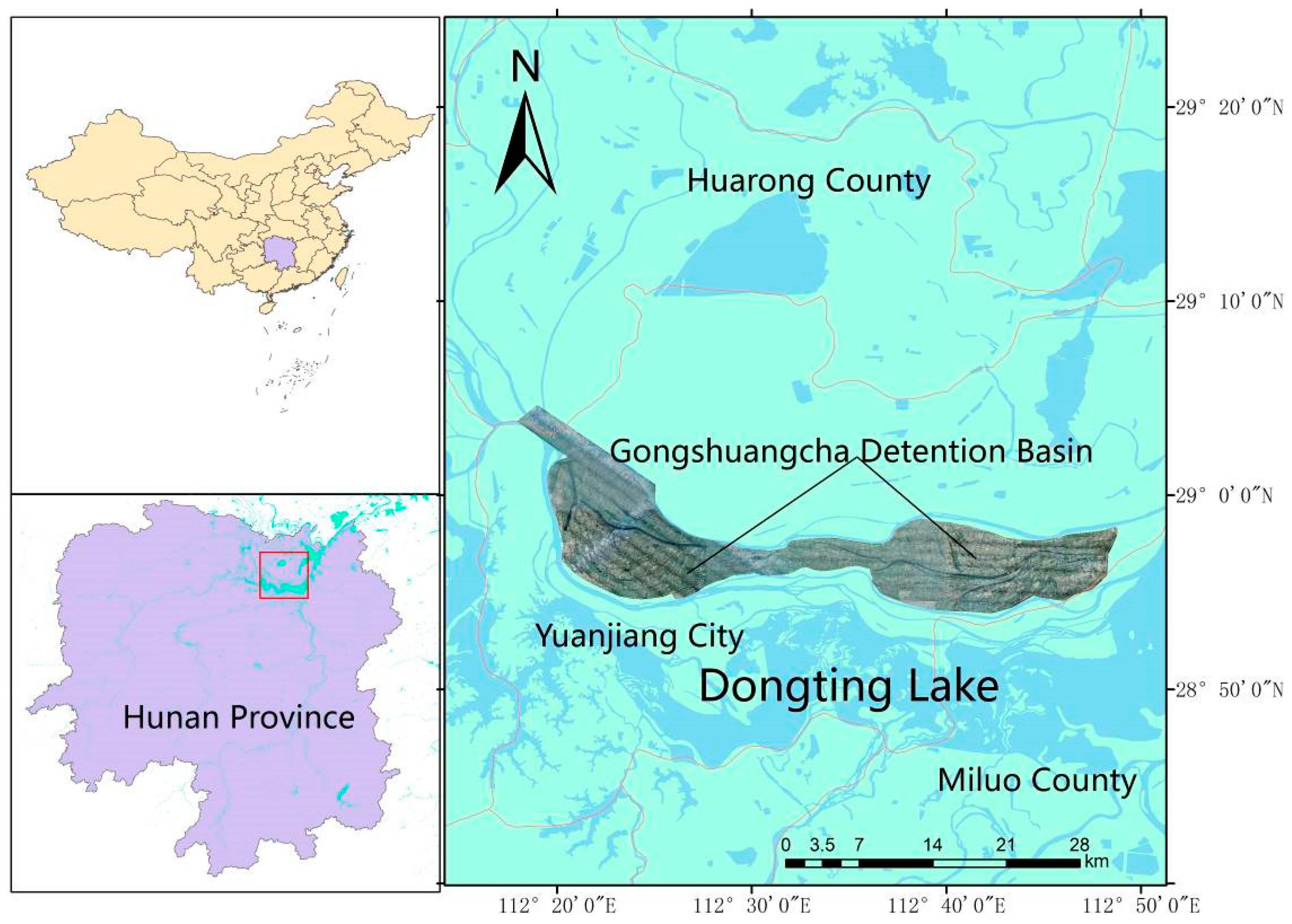
The Gongshuangcha detention basin is one of 24 large flood storage and detention areas in the Dongting Lake area. Located north of Yanjiang City, it is surrounded by water (Figure 1): it borders the Caowei River to the north, the Huangtubao River to the south, Dongting Lake to the east, and Chishan to the west. The flood detention area covers 293.0 km2 (of which cultivated land accounts for 157.6 km2), the total dike length is 121.74 km, and the area’s population is 164,200. Due to its large population, the occurrence of a flood disaster would inevitably cause major losses to the local economy, so it is of great significance to carry out flood damage evaluations in this area.
2.2. Dataset
A HARRIER 68i airborne laser measurement system from TopoSys (TopoSys GmbH, Biberach, Germany) was used for aerial photography and measurement in the study area. The digital camera in the airborne laser measurement system was a Rollei Metric AIC Pro (60 million pixel) from Trimble (Sunnyvale, CA, USA). The inertial navigation system model was an Applanix POS/AV series with a sampling frequency of 200 Hz. The laser scanner model was a Riegl LMS-Q680i with a maximum pulse frequency of 80–400 KHz and a scanning angle of 45/60°.
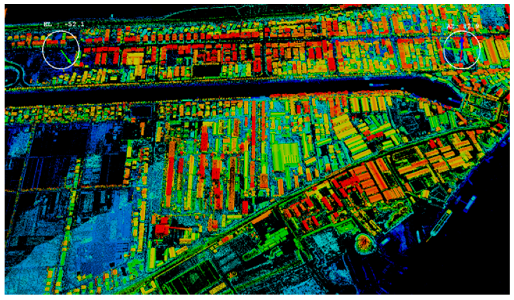
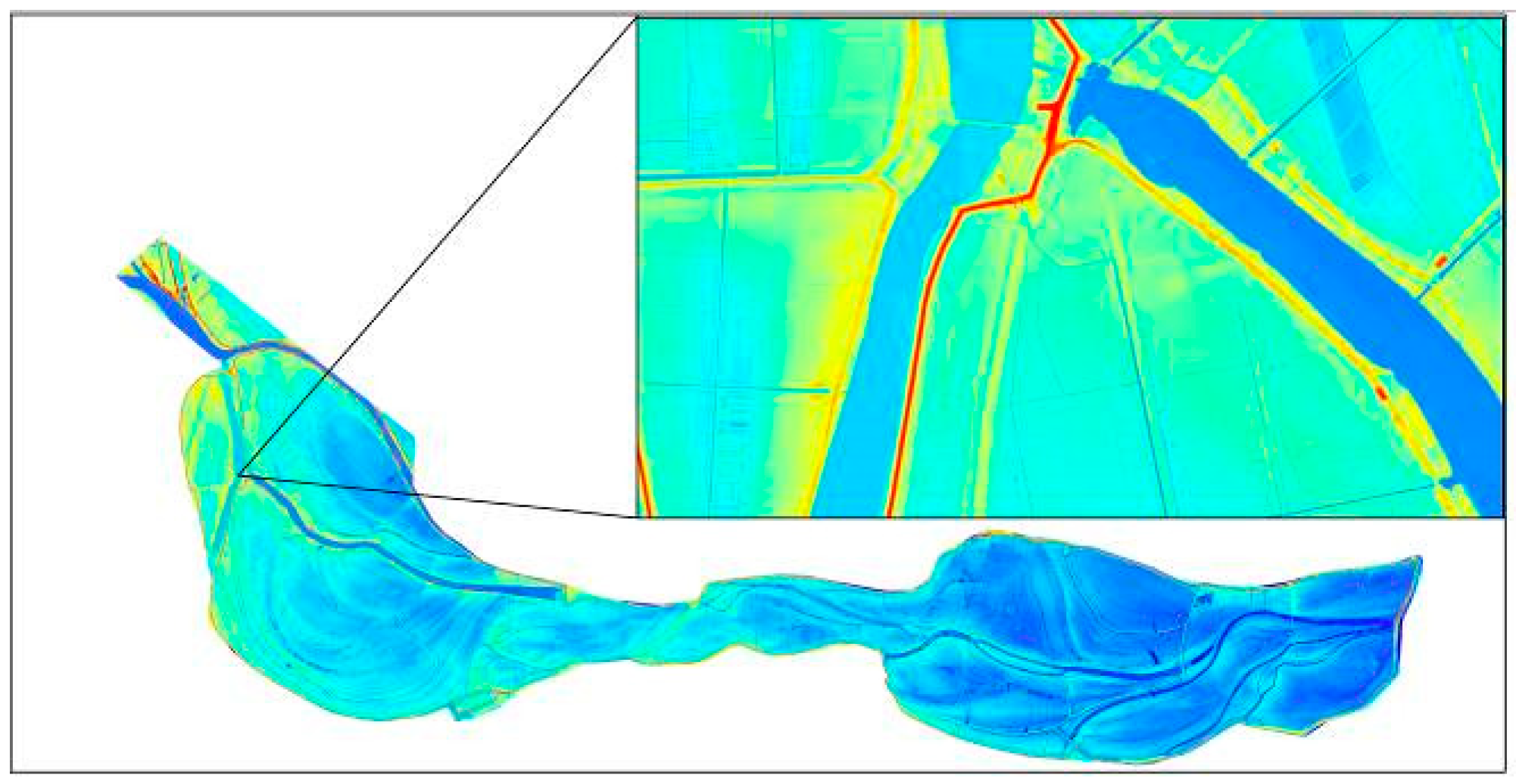
High-resolution DEM data was generated by processing the collected airborne LiDAR point cloud (Figure 2 and Figure 3). The DEM data had a spatial resolution of 1 m and the DEM grid contained 22,000 rows × 51,000 columns. The coordinate system was Beijing Geodetic Coordinate System 1954, and the height system was 1985 National Elevation Benchmarks. Seventy control points were selected on field, the error of DEM was 0.04 m. The overall terrain was relatively flat, with elevations ranging from 4.55 to 45.87 m. Many microtopographic features such as dikes, ditches, and fields were captured by the DEM.
3. Methods
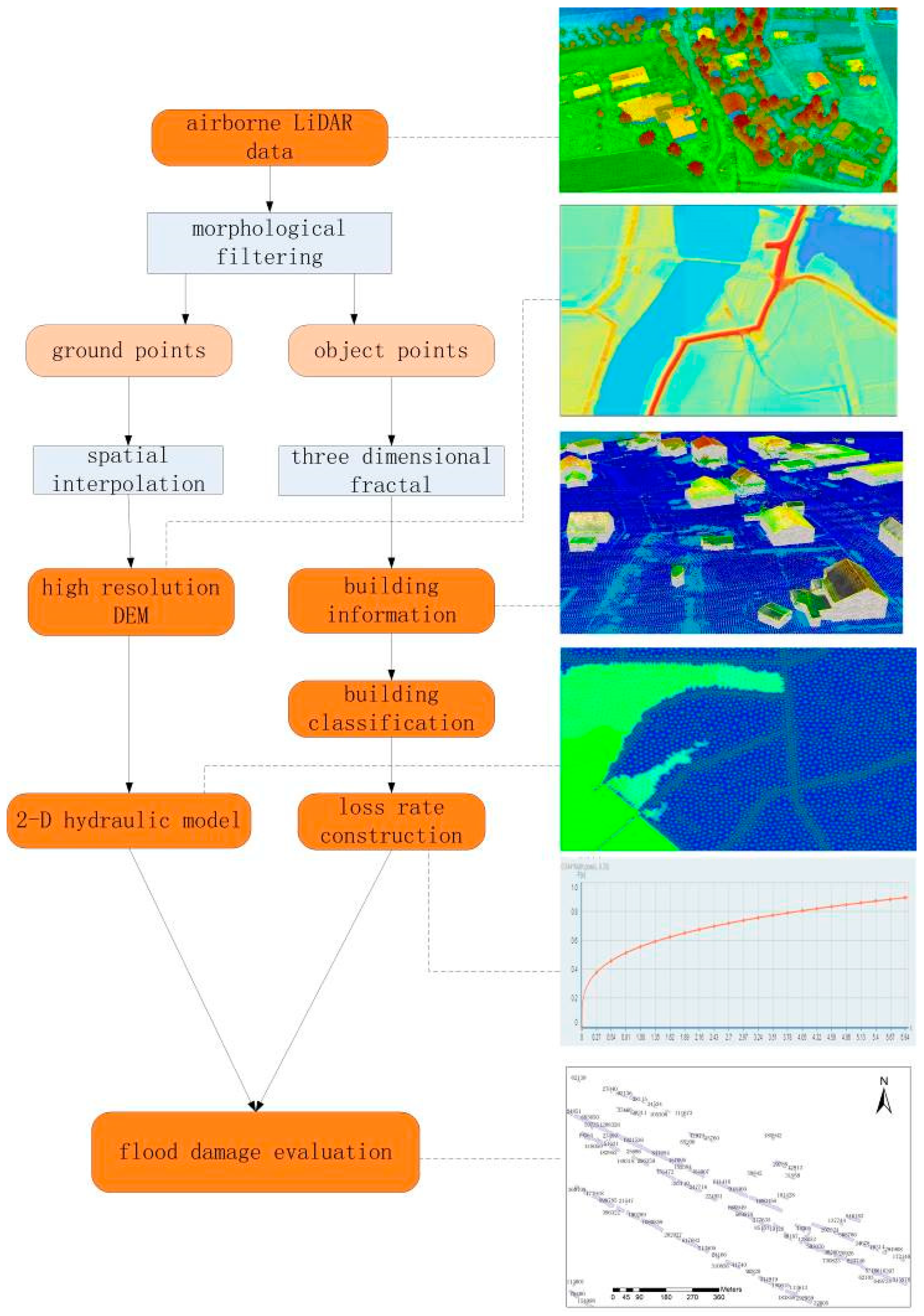
The analytical process followed four main steps (Figure 4):
(1) High-resolution DEM and building information extraction. The ground and object points were separated by LiDAR point cloud morphological filtering. The former were spatially interpolated to generate high-resolution digital terrain. The latter were categorized for high-resolution building vector data; roof outline and height information were included in these data for individual buildings.
(2) Construction of flood routing model. The DEM was used to construct a 2-D flood routing model for the Gongshuangcha detention basin that applied conservative 2-D unsteady flow shallow water equations. The finite volume method and Riemann approximate solution were applied to solve the coupled equations and to simulate the flood routing process in the study area.
(3) Construction of a flood loss rate curve for buildings. Buildings in the study area were classified into two types: brick–wood and brick–concrete structures. Flood loss rate curves for these two types were then fitted based on historical flood damage research data.
(4) Building flood damage evaluation. The value of individual buildings was determined based on their local replacement cost, then integrated with the 2-D flood simulation results and flood loss rate curve to calculate the flood-submerged water depth and flood damage value for each building, respectively. This allowed the overall building losses throughout the study area to be summarized for a given flood event.
3.1. Building Extraction
To extract building information from the airborne LiDAR point cloud, we used the newly proposed 3-D fractal dimension analysis method [33]. The 3-D fractal dimension of each object in the point cloud was calculated based on its unique characteristics, then the obtained 3-D fractal dimension sets were classified. The object points mainly consisted of trees, buildings, and other artificial objects. To extract information for the entire study area, it was first necessary to select representative building point cloud sets by manual interpretation. The range of typical building 3-D fractal dimensions was typically between 1.38 and 1.44; this was then used to extract building information from the entire point cloud.
A total of 33,930 buildings were extracted using this method (Figure 5). According to population data, the three townships in the study area have a total of 38,125 households, showing a good match between the extracted buildings and demographic information. There were two ways for verifying the building classification: one was comparing to high-resolution RS images (for example, excluding patches of trees which were misclassified as buildings); the other was verifying vague objects on RS images by field surveying. After manually omitting 3,379 buildings that were misclassified, 30,551 buildings were correctly identified, an accuracy rate of 90.04%.
3.2. 2-D Hydraulic Model
The flood routing model used 2-D unsteady flow shallow water equations to describe the water flow. First, based on the natural topography and the existing hydraulic structures, the computational area was discretized with an unstructured mesh. Next, the water flow, momentum, and concentration balance were established for each mesh unit by the finite volume method on a time-by-time basis to ensure its conservation. The Riemann approximate solution was used to calculate the normal numerical flux of water flow and momentum across the unit to ensure calculation accuracy. The model has three Riemann approximations to be chosen: Osher, flux vector splitting (FVS), and flux difference splitting (FDS). The model transformed the 2-D problem into a series of local 1-D problems by integral discretization of the finite volume method and rotation invariance of flux coordinates using the following calculation principles:
(1) Basic control equation. The vector expression of the conservative 2-D shallow water equation is [34,35]:
where q = [h,hu,hv]T is the conservative physics vector; f(q) = [hu,hu2+gh2/2,huv]T is the flux vector in the x direction; and g(q) = [hv,huv,hv2+gh2/2]T is the flux vector in the y direction. Here, h is the water depth; u and v are the vertical mean uniform flow velocity components of the x direction and the y direction, respectively; and g is the acceleration of gravity. The source–sink item b(q) is:
where s0x and sfx are the river slope and friction slope in the x direction, respectively; s0y and sfy are the river slope and friction slope in the y direction, respectively; qw is the net rain depth per unit time; and the friction slope in the model is estimated by Manning’s formula.
(2) Discrete equations. The divergence theorem was applied to Equation (1) on any unit Ω for integral discretization, to obtain the basic equation of FVM:
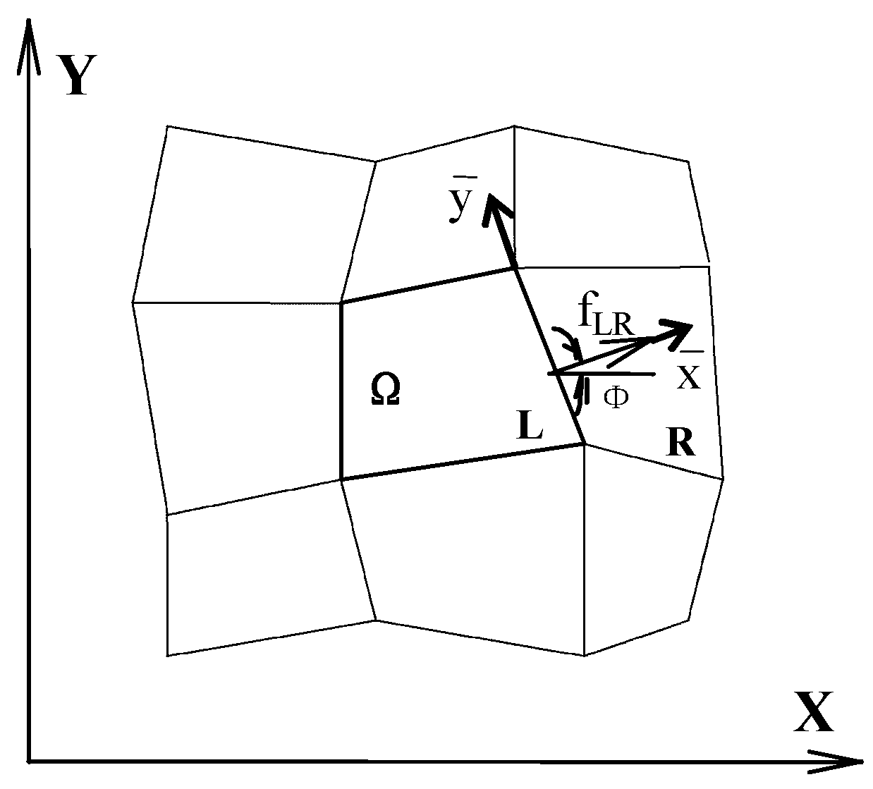
where n is the normal unit vector outside the unit ∂Ω; dω and dL are the area and line integral infinitesimal elements, respectively; and is the normal numerical flux. shows that the solution of normal flux can transform a 2-D problem into a series of local 1-D problems. The finite volume Ω is shown in Figure 6.
Vector q is the average value of units, and it is supposed for the constant when first order. The basic equation of FVM was discretized from Equation (3).
where ; A is the area of unit ; m is the sum of unit sides; Lj is the length of the jth side in the unit; b*(q) is the source term. The flux in the direction normal , in short, is defined as follows:
It is not hard to prove that f(q) and g(q) are invariant to rotation, and meet the following equation:
That is
where is the angle between normal vector n and x. T(Φ) and T(Φ)−1 are the geometrical transform matrix and its inverse matrix, respectively, that is:
could get:
where is transformed from vector q, whose corresponding flow component is normal and tangential directions. Therefore, the key to solving is . Applying the above divergence theorem and flux rotation invariance, the 2-D problem has been transformed into a set of normal direction 1-D problems, which can be solved by partial 1-D problems. Since the q of adjacent units could be different, the q value may be discontinuous on boundaries. The Riemann problem was applied in the model to solve . Partial 1-D Riemann problem is an initial-value problem:
which meets
The origin of is located at the middle point of unit sides, and the direction is in the exterior normal direction. Therefore, is the exterior normal flux at the origin. and are the vector when is at the left and right, respectively. Supposing the initial state when t = 0 is known, solving the Riemann problem, it is obtained that the origin is located at . There are three common ways to estimate normal flux :
1) Arithmetic average: the average of unit fluxes on both sides of common border = [f()+f()]/2, or using the average of physically conserved quantity on both sides, calculate the flux = f([+]/2).
2) Various monotonicity types: such as Total Variation Descent (TVD), Flux-Corrected Transport Algorithm (FCT), and so forth.
3) Riemann approximates based on Eigen theory: Flux Vector Splitting (FVS), Flux Difference Splitting (FDS), and Osher.
A flood process simulation program was written based on the above model principles (Figure 7). All the three estimation ways were applied in the model for flood coupling solution. The program was able to choose any of them when needed.
(3) Boundary conditions. The model determined five types of water flow boundaries: the land boundary, the open boundary of slow and rapid flow, the inner boundary, the dynamic boundary of water exchange, and the wetland tributary boundary.
(4) Solution of the equations. The equations belong to an explicit scheme discretization and are solved by time-interval iteration.
According to the ‘Feasibility Study Report on the Flood Diversion and Storage Project of Qianliang Lake, Gongshuangcha and East Dyke of Datonghu in the Dongting Lake Area’ approved by the China Ministry of Water Resources in 2009, during typical flooding events in 1954, 1966, and 1998, when the incoming flood flow in the three flood storage areas was 8000–12,000 m3/s, the water level impact was minimum on Chenglingji. For the 30-year flood in 1954, the study determined that the maximum flood discharge flow of the Gongshuangcha flood diversion sluice was 3630 m3/s and the designed flood discharge water level was 33.10 m.
We simulated the flood routing process by using this sluice to control flood discharge, setting its flood discharge hydrograph as the input condition for model calculation. The following conditions were set: when the water level (H) was <31.63 m, the flow was at the free outflow stage and its rate was 3630 m3/s; when 31.63 < H < 32.60 m, the flow was at the submerged outflow stage and its rate was 3050 m3/s; when 32.60 < H < 33.65 m, a temporary flood diversion sluice was required.
The 2-D hydraulic model mesh was an unstructured triangulation with a total of 83,378 triangular units. Using the 1 m resolution DEM data, nearest-neighbor interpolation was used to obtain the elevation of each triangle apex and center point as the initial condition for model calculation. A flood submerged process of four days and three hours was simulated, and the flood storage and detention area was eventually completely submerged (Figure 7).
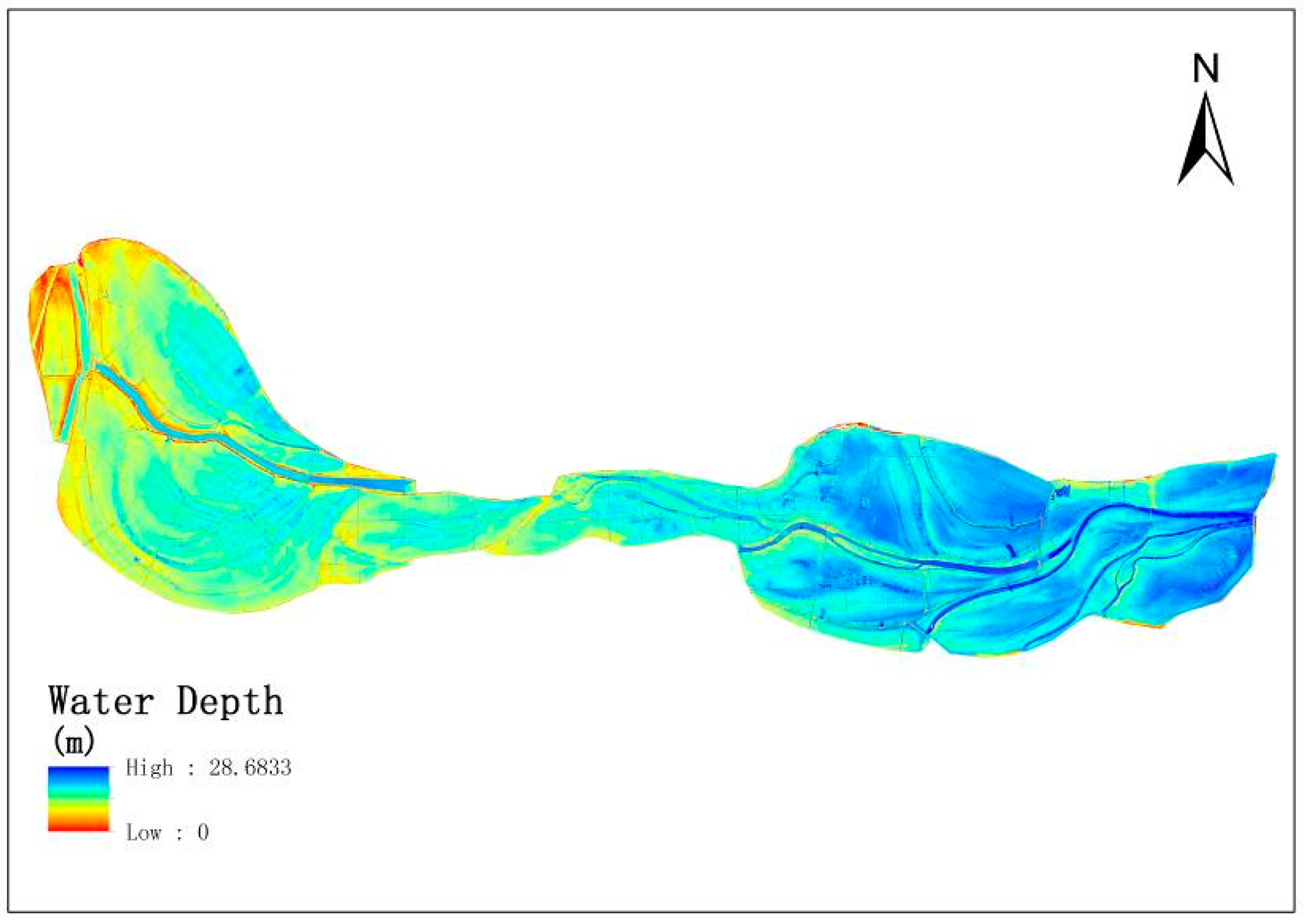
The final completely submerged water depth data (Figure 8) were used for building flood damage calculations. The flooding depth in the eastern part of Gongshuangcha was generally deep, while the west (farther from the inflow sluice) was relatively shallow.
3.3. Construction of Building Flood Loss Rate Curves
Different building materials vary in their ability to withstand floodwater, which is reflected in building flood loss rates, making it necessary to classify all buildings in the study area.
3.3.1. Building Classification
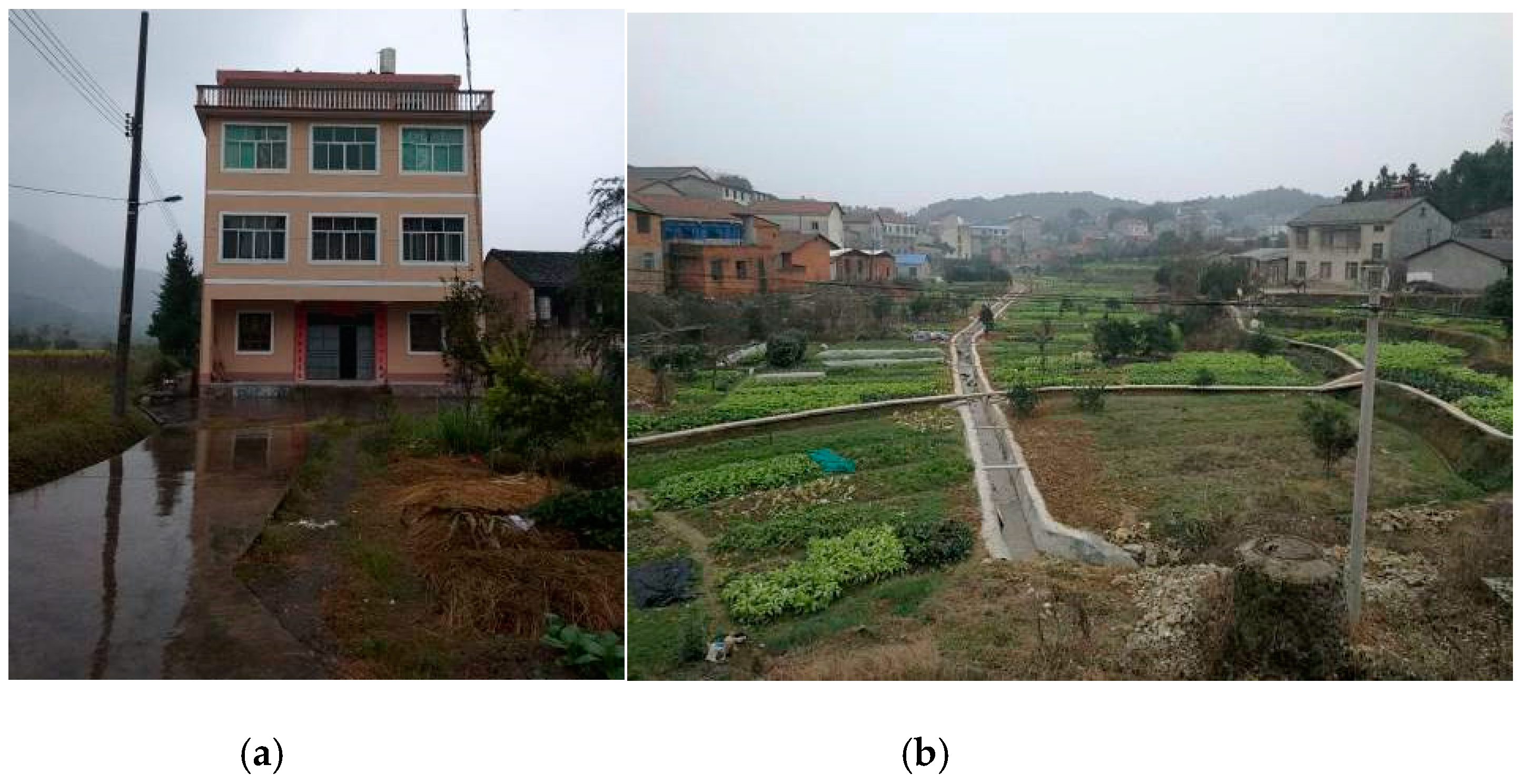
As a typical rural area in the middle reaches of the Yangtze River, the buildings in Gongshuangcha consist of two main types: brick–concrete (Figure 9a) and brick–wood (Figure 9b). The former are mainly distributed in township municipal centers while the latter are widely distributed in rural residential areas; these are the most numerous and typical in the study area.
The roofs of brick–wood buildings are mainly sloped tile, while those of brick–concrete buildings are mainly flat. However, it is difficult to distinguish the two by roof features and there is no strict division between them. A more suitable differentiation method is based on the building’s number of floors. Brick–concrete structures usually have three or more floors, while brick–wood structures in most rural areas usually have one to two floors. The Ministry of Housing and Urban–Rural Development of China issued the ‘Design Code for Residential Buildings’ (GB 50096-2011) in 2011, which specifies that the average residential floor height should be 2.8 m and the net indoor height should not be lower than 2.4 m [36]. Based on these specifications and using an average floor height of 3 m, buildings below 6 m height were classified as brick–wood and those over 6 m were classified as brick–concrete. The building classification and floor number calculations are as follows:
where H is the height of the building and In represents the rounded value without the decimal point. The difference between the elevation of the roof and the terrain is the height of the building.
Brick–wood building: H < 6 m, number of floors: In(H/3)+1;
Brick–concrete building: H ≥ 6 m, number of floors: In(H/3)+1;
Based on the above method, 19,879 brick–wood buildings and 10,672 brick–concrete buildings were identified (Table 1). Two-story buildings accounted for 92% of the brick–wood structures, consistent with current rural housing construction practices. The height of brick–concrete structures mostly ranged from 6 to 18 m; few buildings had more than 6 floors.
3.3.2. Establishment of Flood Loss Rate
The flood loss rate of buildings refers to the ratio of postflood building value loss to its preflood value. In practice, the predisaster value of buildings is usually considered to be the replacement cost, the estimated value of damaged buildings that need to be rebuilt. The flood loss rate is the result of multiple flood factors, though under the action of a single factor, it usually meets the trend of an exponential curve. The general statistical regression model of building flood loss rate is calculated as [37]:
where Y is the flood loss rate; is the flood characteristic factor, including depth, duration, flow rate, sediment content, and so forth; and , are parameters that must be solved through typical survey or experimental data statistical regression.
For A, if only the submerged water depth H is considered, then the statistical regression model becomes:
To facilitate the use of multiple linear regression to solve the parameters, Equation (13) needs to be logarithmic transformed on both sides:
If ; ; and , then the equation becomes:
This is a binary equation with h as the independent variable and y as the dependent variable, in which parameters a and c1 can be obtained by linear regression.
Table 2 shows flood damage statistics for buildings in the study area in the early 1990s, in which it can be assumed that rural houses were mostly brick–wood while urban houses were mostly brick–concrete. Thus, in our multiple regression analysis, these rural house data were used to calculate the flood loss rate of brick–wood buildings, while urban house data were used for brick–concrete buildings.
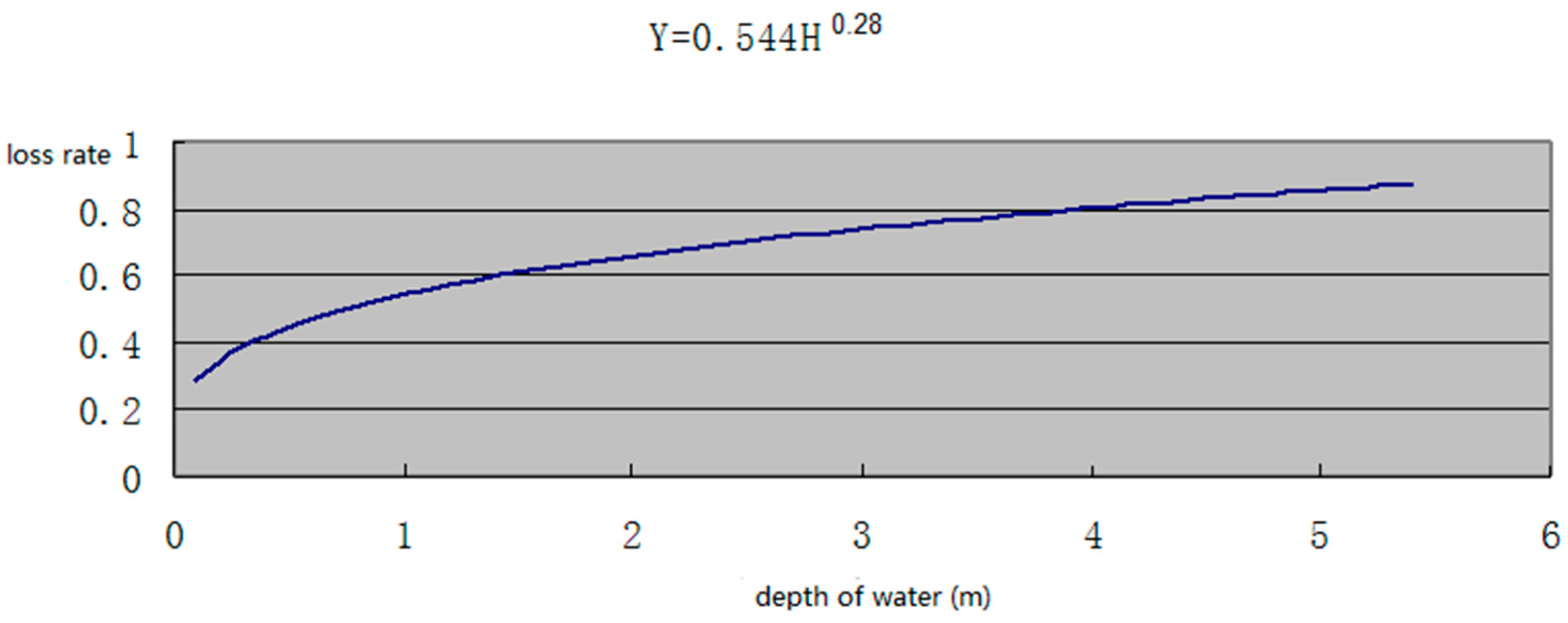
From Table 2, the two calculated building types and are as follows:
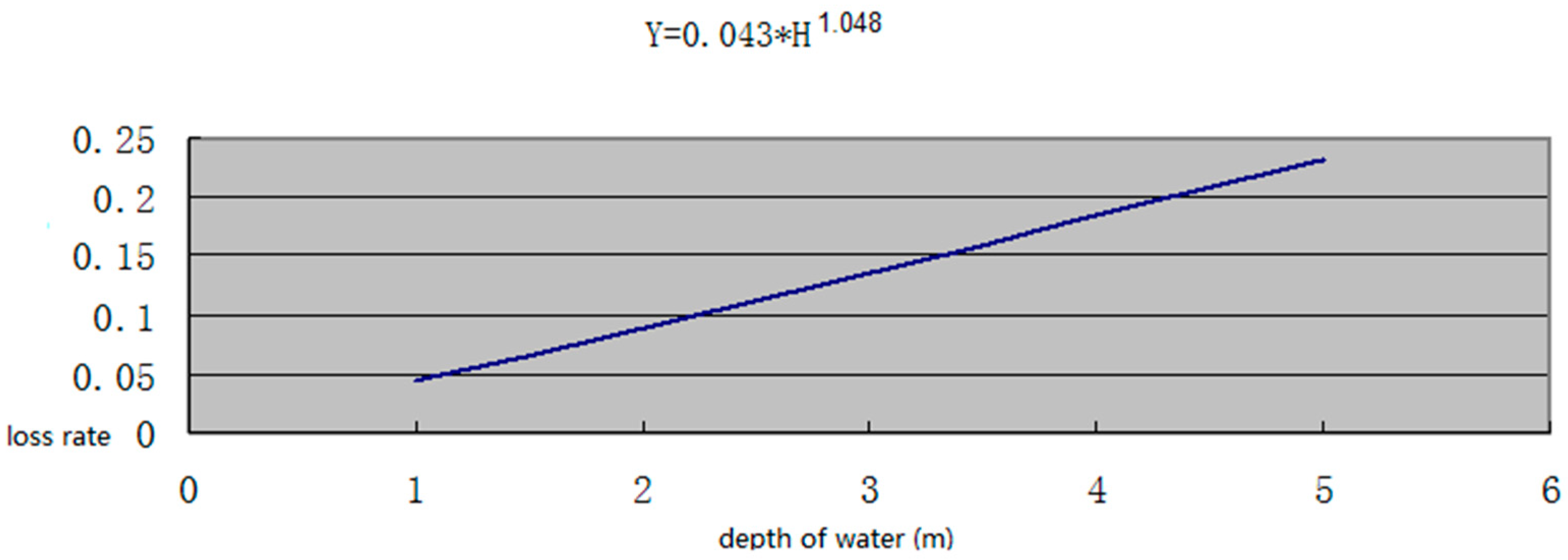
which is , where and are the flood loss rate relations of brick–wood and brick–concrete buildings, respectively. Using these, the relation curves of flood loss rates for brick–wood and brick–concrete buildings are shown in Figure 10 and Figure 11, respectively. Limited by the data collected (Table 2), only loss rate when water depth was no more than 5 m was fitted in the curves. The loss rate when water depth was above 6 m needs to be calculated by extending the curve.
3.4. Calculation of Building Replacement Cost
Two statistical methods can be used to evaluate the predisaster value of a building. One is the current market price of the building, especially as this is greatly affected by the real estate market. The other is the cost of rebuilding, also known as replacement cost. Since postdisaster recovery work mainly involves building reconstruction and renovation, it is more reasonable to estimate the predisaster value using replacement cost.
In rural areas, brick–concrete buildings are usually contracted to professional construction companies and their construction costs are subject to specific budget standards. The study area’s local government provided the standard cost index for brick–concrete buildings, which specified the standard engineering formwork and bill of quantities from which a budget can be generated based on local manpower, materials, and equipment rates. The cost index mainly includes an overview of sample construction characteristics as well as the main material costs per square meter and labor costs. Using this, the replacement cost per square meter of local brick–concrete buildings in recent years was about 1566 yuan. Since the cost of construction does not fluctuate annually, we used this cost as the replacement cost for brick–concrete buildings.
In contrast, brick–wood buildings are usually built by individual households. According to guidance documents on the cost of brick–wood buildings issued by the local Price Bureau and Real Estate Administration, such buildings are divided into grades 1 and 2, and also into residential and nonresidential categories. Construction costs, which include civil engineering and interior finish fees, are about 600 yuan per square meter. Other costs, which include the construction registration fee, survey and design, preconstruction cost, and infrastructure construction fee, are about 350 yuan per square meter. The guidance document states that the house replacement cost includes all of these costs. Similar to the replacement cost of brick–concrete buildings, we only considered the construction cost, so the replacement cost of brick–wood buildings was set at 600 yuan per square meter in this study.
4. Results and Discussion
4.1. Results
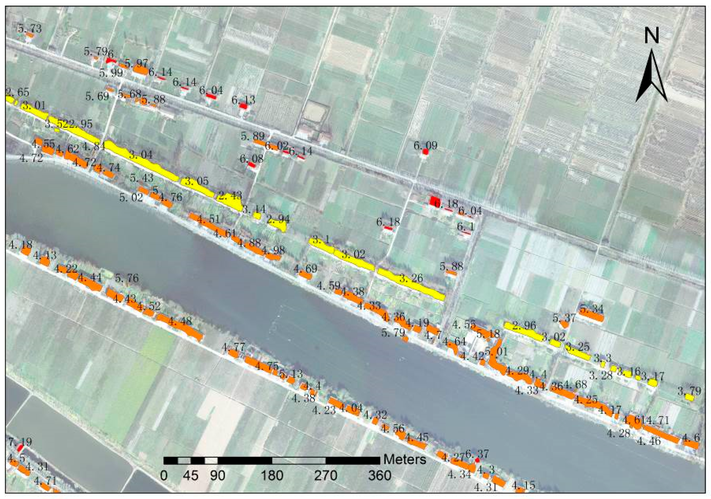
For a single building, the DEM grid inside the building may be completely submerged, partially submerged, or completely unsubmerged. The first and last cases are relatively simple, while a partially submerged situation indicates that the building is located at the boundary of the flood water. In this case, it is more appropriate to consider this as submerged. Thus, the submerged depth of the building can be obtained by Hwater level = Max(Hcell1 + Hcell2 + …… + Hcelln)/n, where n is the number of DEM cells inside the building and Hcelln is the water depth of the nth cell inside the building. Using this approach, the flood statistics for brick–concrete and brick–wood buildings at different water depths are shown in Table 3 and an example map is given in Figure 12.
The total replacement cost for brick–wood and brick–concrete buildings can be calculated as the product of the cost per square meter and the building area as follows:
where Fbrick−wood and Fbrick−concrete represent the number of floors; H is the building height; Pbrick−wood and Pbrick−concrete are the per square meter replacement cost in yuan; and Abrick−wood and Abrick−concrete represent the footprint area of a single building. In this study, the feature roof coordinate points were expressed in 3-D coordinate points and the polygon area formed by the plane projection coordinates can be used to obtain the footprint area of the building.
Combined with these flood loss rate functions, the flood damage equation for a single building can be obtained as follows:
where Ybrick−wood and Ybrick−concrete represent the flood loss rate function and H is the submerged water depth. Finally, the building flood damage in the study area can be calculated as follows:
where m and n represent the number of brick–wood and brick–concrete buildings, respectively.
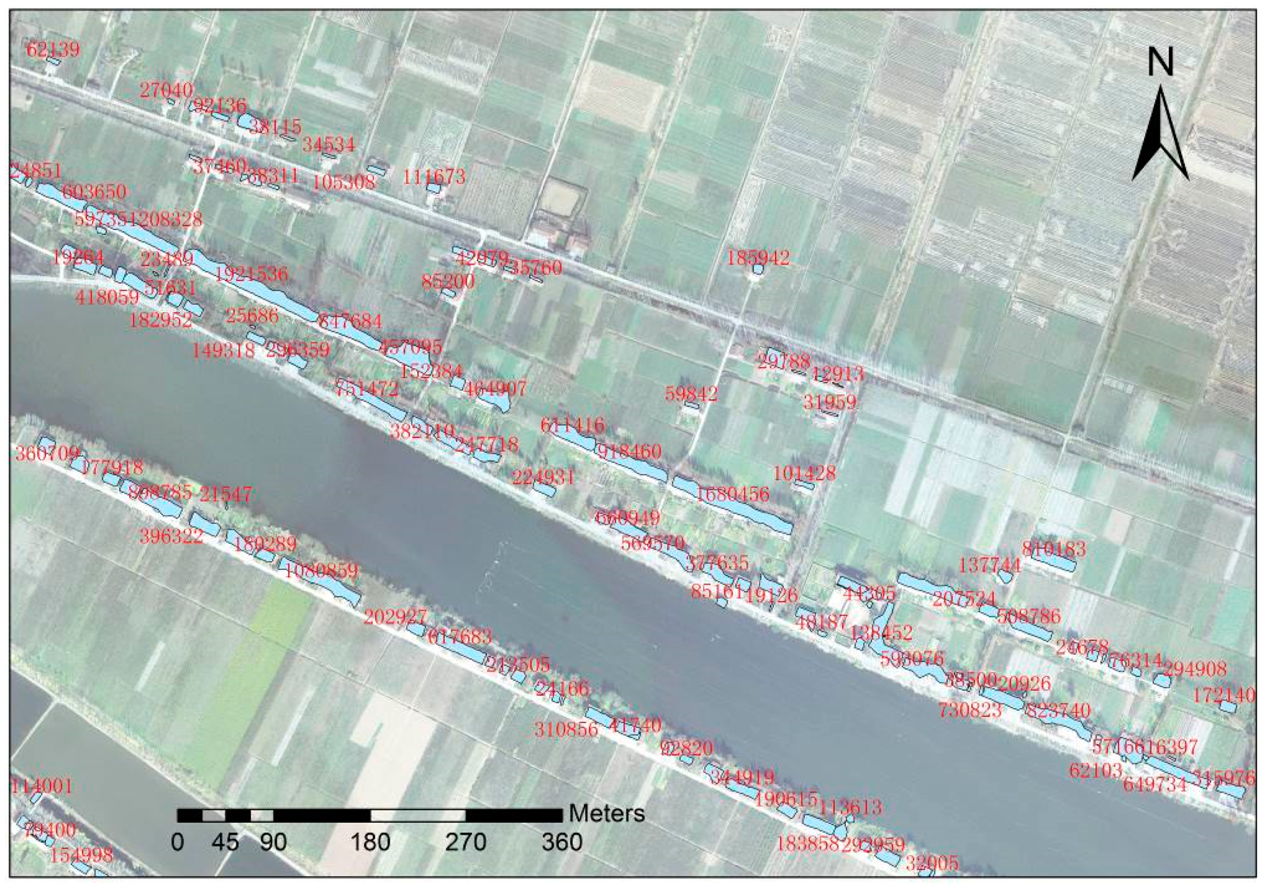
Based on the above equations, when the study area was fully submerged by floodwater, the flood damage of brick–wood buildings reached 3.358 billion yuan and that of brick–concrete buildings reached 1.686 billion yuan for a total loss of 5.044 billion yuan. Figure 13 shows an example of a final flood loss map.
4.2. Discussion
The flood building damage and loss evaluation framework presented in this paper is practical, and can be feasibly applied to other regions. This evaluation method is formed of LiDAR building extraction and classification, 2-D hydraulic model, and flood loss rate curve of buildings. All three parts are based on extensive research.
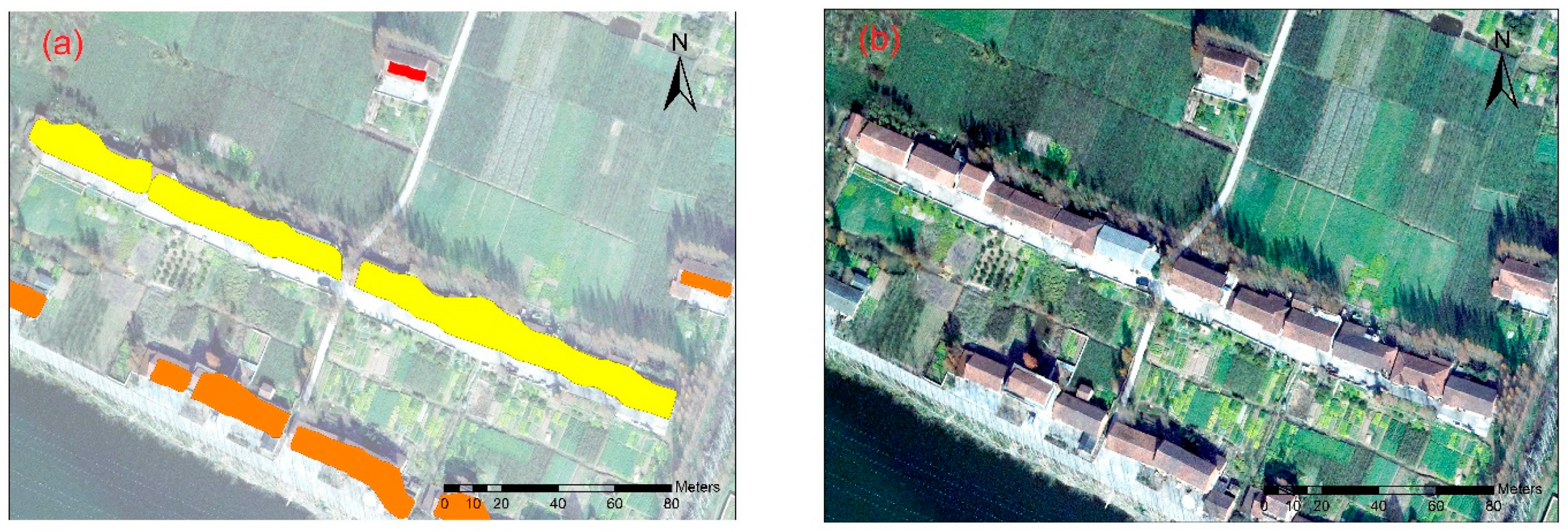
For building extraction from LiDAR point clouds, various building extraction algorithms have been proposed, such as Bayesian self-adaption network [38], K-means clustering method [39], and region growing clustering [40]. In this research, a 3-D fractal dimension analysis method presented by us [33] was used. Other building extraction methods can also be used in this part. The accuracy of building information is essential for proper flood damage evaluations, but it is challenging to extract these data from airborne LiDAR point clouds. For example, some rural houses in the study area were too close to each other to be easily separated by an algorithm, resulting in multiple houses being represented by a single vector polygon (Figure 14). Although this is essentially negligible for the large-scale calculation of overall flood damage, it still causes errors when analyzing individual objects. In addition, some multistory buildings have complex designs, such as terraces, that can complicate this process. Therefore, further postprocessing is required to properly separate and assess such buildings for improved accuracy.
The research area is located in the Yangtze River basin. Flood storage and detention areas there are normally protected by levees. As long as the levees are not burst, the areas are under full protection from flood. However, once levees are burst (such as flood discharge in this case study), the water can reach up to meters deep. Ding [37] collected flood loss rate in flood storage and detention areas of the Yangtze River basin released by water administration institutions (Table 4), most of which are from the 1980s and 1990s. In the field of flood loss evaluation, the application has been a slow progress. Levels of water depth were not considered in the table, and statistics were generalized and grouped by industries. The data is hard to be used in this research.
In terms of setting proper flood loss rate curves, as there is no official organization in China that issues technical standards for this purpose, we used historical flood damage data and simulated the flood loss rate. In addition, at present there is no clear method for carrying out experimental simulations and calculations on the actual flood resistance of buildings, such as analyzing how soon different types of buildings will collapse after flooding and the damage to buildings at different flow rates. These subjects are incredibly challenging and are worthy of further development in future research. Generally speaking, further works of flood prevention should be carried out by water administration institutions in China. More efforts should be conducted in, for example, setting up flood loss historical datasets, flood loss rate databases, flood loss evaluation models and software, and so forth. In this research, we attempted to evaluate flood-related building loss based on airborne LiDAR data and 2-D hydraulic models, using updated methods and technologies in industry application. We hope the application of those technologies could contribute to flood loss evaluation of small-scale and single objects.
5. Conclusions
Building damage evaluation is of great significance for quickly, efficiently, and accurately assessing flood damage. This study tested a proposed technical framework with broad applicability that extracts and classifies building information based on airborne LiDAR data, constructs a building flood loss rate model based on a 2-D hydraulic model, and calculates potential building flood damage.
Flood damage evaluation at small scales and for individual objects is becoming a new research trend. In particular, the development of new surveying and remote sensing techniques has greatly improved the extraction accuracy for ground objects and terrain. Refined spatio-temporal flood simulations and accurate flood damage evaluations have become common demands from modern flood management departments. This study’s use of an airborne LiDAR point cloud to obtain building information and quickly evaluate damage using the constructed loss rate curve demonstrates a feasible method, especially for vast rural areas. As the gaps between houses tend to be relatively large in such areas, the point cloud can more easily distinguish individual buildings in order to carry out predisaster evaluations of flood damage potential over large areas. This method also has the potential to evaluate flood damage for other infrastructure with similar characteristics, including railways, highways, farmland, and towers.
Author Contributions
D.S. and T.Q. conducted the primary experiments and cartography and analyzed the results. D.S., W.C., and Y.C. offered data support for this work. J.W. provided the original idea for this paper.
Funding
This research was funded by National Key R&D Program of China (grant number 2018YFC0407805), National Natural Science Foundation of China (grant number 41501558, 41871294) and Key Technology Application and Demonstration of Water Conservation Society Innovation Pilot In Jinhua, Zhejiang (grant number SF-201801).
Conflicts of Interest
The authors declare no conflict of interest.
References
- Lekuthai, A.; Vongvisessomjai, S. Intangible Flood Damage Quantification. Water Resour. Manag. 2001, 15, 343–362. [Google Scholar] [CrossRef]
- Jonkman, S.N. Loss of Life Estimation in Flood Risk Assessment. Ph.D. Thesis, Delft University, Delft, The Netherlands, 2007. [Google Scholar]
- Tapsell, S.M.; Penning-Rowsell, E.C.; Tunstall, S.M.; Wilson, T.L. Vunerability to flooding: Health and social dimensions. Philos. Trans. R. Soc. A 2002, 360, 1511–1525. [Google Scholar] [CrossRef] [PubMed]
- Hajat, S.; Ebi, K.L.; Kovats, S.; Menne, B.; Edwards, S.; Haines, A. The human health consequnences of flooding in Europe and the implication for public health: A review of the evidence. Appl. Environ. Sci. Public Health 2003, 1, 13–21. [Google Scholar]
- Ahern, M.; Kovats, S.; Wilkinson, P.; Few, R.; Matthies, F. Global health impacts of floods: Epidemiologic evidence. Epidemiol. Rev. 2005, 27, 36–46. [Google Scholar] [CrossRef] [PubMed]
- Merz, B.; Kreibich, H.; Schwarze, R.; Thieken, A. Review article “Assessment of Economic Flood Damage”. Nat. Hazard. Earth Syst. 2010, 10, 1697–1724. [Google Scholar] [CrossRef]
- Moore, M.R. Development of a High-Resolution 1D/2D Coupled Flood Simulation of Charles City, Iowa. Master’s Thesis, University of Iowa, Iowa City, IA, USA, 2011; pp. 49–68. [Google Scholar]
- MURL (Ministerium fur Umwelt, Raumordnug und Land-wirtschaft des Landes Nordrhein-Westfalen). Potentielle Hochwasserschaden am Rhein in Nordrhein-Westfalen Dusseldorf; MURL: Düsseldorf, Germany, 2000. [Google Scholar]
- ICPR (International Commission for the Protection of the Rhine). Non Structural Flood Plain Management, Measures and Their Effectiveness; International Commission for the Protection of the Rhine: Koblenz, Germany, 2002. [Google Scholar]
- FEMA (Federal Emergency Management Agency). HAZUS: Multi-Hazard Loss Estimation Model Methodology-Flood Model; FEMA: Washington, WC, USA, 2003.
- Apel, H.; Aronica, G.T.; Kreibich, H.; Thieken, A.H. Flood risk analyses-how detailed do we need to be? Nat. Hazards 2009, 49, 79–98. [Google Scholar] [CrossRef]
- Huang, Z.; Zhou, J.; Song, L.; Lu, Y.; Zhang, Y. Flood disaster loss comprehensive evaluation model based on optimization support vector machine. Expert Syst. Appl. 2010, 37, 3810–3814. [Google Scholar] [CrossRef]
- Ranger, N.; Hallegatte, S.; Bhattacharya, S.; Bachu, M.; Priya, S.; Dhore, K.; Rafique, F.; Mathur, P.; Naville, N.; Henriet, F.; et al. An assessment of the potential impact of climate change on flood risk in Mumbai. Clim. Chang. 2011, 104, 139–167. [Google Scholar] [CrossRef]
- Van Dyck, J.; Willems, P. Probalistic flood risk assessment over large geographical regions. Water Resour. Res. 2013, 49, 3330–3344. [Google Scholar] [CrossRef]
- Prettenthaler, F.; Amrusch, P.; Habsburg-Lothringen, C. Estimation of an absolute flood damage curve based on an Austrian case study under a dam breach scenario. Nat. Hazards Earth Syst. 2010, 10, 881–894. [Google Scholar] [CrossRef] [Green Version]
- Bouwer, L.M.; Bubeck, P.; Wagtendonk, A.J.; Aerts, J.C.J.H. Iundation scenarios for flood damage evaluation in polder areas. Nat. Hazards Earth Syst. 2009, 9, 1995–2007. [Google Scholar] [CrossRef]
- Pistrika, A. Flood Damage Estimation based on Flood Simulation Scenarios and a GIS Platform. Eur. Water 2010, 30, 3–11. [Google Scholar]
- Ward, P.J.; Marfai, M.A.; Yulianto, F.; Hizbaron, D.R.; Aerts, J.C.J.H. Coastal inundation and damage exposure estimation: A case study for Jakarta. Nat. Hazards 2011, 56, 899–916. [Google Scholar] [CrossRef]
- Muhammad, M.; Takeuchi, K. Assessment of flood hazard, vulnerability and risk of mid-eastern Dhaka using DEM and 1D hydrodynamic model. Nat. Hazards 2012, 61, 757–770. [Google Scholar]
- Ernst, J.; Dewals, B.J.; Detrembleur, D.S.; Archambeau, P.; Erpicum, S.; Pirotton, M. Micro-scale flood rsik analysis based on detailed 2D hydraulic modeling and high resolution geographic data. Nat. Hazards 2010, 55, 181–209. [Google Scholar] [CrossRef]
- Mongkonkerd, S.; Hirunsalee, S.; Kanegae, H.; Denpaiboon, C. Comparison of Direct Monetary Flood Damage in 2011 to Pillar House and Non-Pillar House in Ayutthaya, Thailand. Procedia Environ. Sci. 2013, 17, 327–336. [Google Scholar] [CrossRef]
- Thieken, A.H.; Kreibich, H.; Muller, M.; Merz, B. Coping with floods: Preparedness, response and recovery of flood-affected residents in Germany in 2002. Hydrol. Sci. J. 2007, 52, 1016–1037. [Google Scholar] [CrossRef]
- Kreibich, H.; Piroth, K.; Seifert, I.; Maiwald, H.; Kunert, U.; Schwarz, J.; Merz, B.; Thieken, A.H. Is flow velocity a significant parameter in flood damage modelling? Nat. Hazards Earth Syst. 2009, 9, 1679–1692. [Google Scholar] [CrossRef] [Green Version]
- Boettle, M.; Kropp, P.; Reiber, L.; Roithmeier, O. About the influence of elevation model quality and small-sacle damage functions on flood damage estmation. Nat. Hazards Earth Syst. 2013, 11, 3327–3334. [Google Scholar] [CrossRef]
- Yang, Y.C.E.; Ray, P.A.; Brown, C.M.; Khalil, A.F.; Yu, W.H. Estimation of flood damage functions for river basin planning: A case study in Bangladesh. Nat. Hazards 2015, 75, 2773–2791. [Google Scholar] [CrossRef]
- Sanders, B.F. Evaluation of on-line DEMs for flood inundation modeling. Adv. Water Resour. 2007, 30, 1831–1843. [Google Scholar] [CrossRef]
- Sampson, C.C.; Fewtrell, T.J.; Duncan, A.; Shaad, K.; Horrit, M.S.; Bates, P.D. Use of terrestrial laser data to drive decimetric resolution urban inundation models. Adv. Water Resour. 2012, 14, 1–17. [Google Scholar] [CrossRef]
- Meesuk, V.; Vojinovic, Z.; Mynett, A.E.; Abdullah, A.F. Urban flood modelling combining top-view LiDAR data with ground-view SfM observations. Adv. Water Resour. 2015, 75, 105–117. [Google Scholar] [CrossRef]
- McCarthy, S.; Tunstall, S.; Parker, D.; Faulkner, H.; Howe, J. Risk communication in emergency response to a simulated extreme flood. Environ. Hazards 2007, 7, 179–192. [Google Scholar] [CrossRef] [Green Version]
- Leskens, J.G.; Brugnach, M.; Hoekstra, A.Y.; Schuurmans, W. Why are decisions in flood disaster management so poorly supported by information from flood models? Environ. Modell. Softw. 2014, 53, 53–61. [Google Scholar] [CrossRef]
- Gerl, T.; Bochow, M.; Kreibich, H. Flood Damage Modeling on the Basis of Urban Structure Mapping Using High-Resolution Remote Sesing Data. Water 2014, 6, 2367–2393. [Google Scholar] [CrossRef]
- Molinari, D.; Scorzini, A.R. On the Influence of Input Data Quality to Flood Damage Estimation: The Performance of the INSYDE Model. Water 2017, 9, 688. [Google Scholar] [CrossRef]
- Yang, H.; Chen, W.; Qian, T.; Shen, D.; Wang, J. The Extraction of Vegetation Points from LiDAR Using 3D Fractal Dimension Analyses. Remote Sens. 2015, 7, 10815–10831. [Google Scholar] [CrossRef] [Green Version]
- Liang, Q.; Borthwick, A.G.L. Adaptive quadtree simulation of shallow flows with wet–dry fronts over complex topography. Comput. Fluids 2009, 38, 221–234. [Google Scholar] [CrossRef]
- Wang, Y.; Liang, Q.; Kresserwani, G.; Hall, J.W. A 2D shallow flow model for practical dam-break simulations. J. Hydraul. Res. 2011, 49, 307–316. [Google Scholar] [CrossRef]
- Design Code for Residential Buildings; GB 50096-2011; Ministry of Housing and Urban-Rural Development of China: Beijing, China, 2011.
- Ding, Z. A Study on the Technology and Method of Flood and Waterlogging Disaster Loss Assessment Based on RS and GIS. Ph.D. Thesis, China Institute of Water Resources and Hydropower Research, Beijing, China, 2004; pp. 63–80. [Google Scholar]
- Brunn, A.; Weidner, U. Hierarchical Bayesian nets for building extraction using dense digital surface models. ISPRS J. Photogramm. 1998, 53, 296–307. [Google Scholar] [CrossRef]
- Elberink, E.O.; Maas, H. The use of anisotropic height texture measures for the segmentation of airborne laser scanner data. Int. Arch. Photogram. Remote Sens. 2000, 33, 678–684. [Google Scholar]
- Tóvári, D.; Vögtle, T. Object Classification in Laser Scanning Data. Int. Arch. Photogramm. Remote Sens. 2012, 36, 45–49. [Google Scholar]
- Changjiang Water Resources Commission. Estimation of Flood Loss in Jingjiang Flood Diversion Area; Changjiang Water Resources Commission: Wuhan, China, 1983. [Google Scholar]
- Engineering Administration Bureau of Jingjiang Flood Diversion and Storage Area. Basic Data Collection of Jingjiang Flood Diversion Area; Engineering Administration Bureau of Jingjiang Flood Diversion and Storage Area: Jingzhou, China, 1991. [Google Scholar]
- Changjiang Water Resources Commission. A Brief Analysis of the Economic Loss of Flood Diversion and Storage in the Middle Reaches of the Yangtze River; Changjiang Water Resources Commission: Wuhan, China, 1987. [Google Scholar]
- Office of Flood Control and Drought Relief, Changjiang Water Resources Commission. Flood Storage and Detention Areas in the Middle and Lower Reaches of the Yangtze River; Office of Flood Control and Drought Relief, Changjiang Water Resources Commission: Wuhan, China, 1990. [Google Scholar]
- Changjiang Water Resources Commission. Investigation and Analysis of Economic Loss of Flood Distribution and Storage in the Middle Reaches of the Yangtze River; Changjiang Water Resources Commission: Wuhan, China, 1990. [Google Scholar]
- Hubei Provincial Water Resources and Hydropower Planning Survey and Design Institute. Benefit Calculation of Flood Control Project in Hanjiang Plain and Honghu Lake; Hubei Provincial Water Resources and Hydropower Planning Survey and Design Institute: Wuhan, China, 1989. [Google Scholar]
Figure 1.
The location of the Gongshuangcha detention basin in the Dongting Lake area.

Figure 2.
Example of airborne LiDAR point cloud.

Figure 3.
Example of high-resolution DEM data.

Figure 4.
Flow chart of analytical process.

Figure 5.
(a) Extracted building information and (b) detailed example (red box in (a)).

Figure 6.
The finite volume Ω. is left side of boundary, is right side of the boundary, is flux, is the angle in the normal direction of the boundary.
Figure 6.
The finite volume Ω. is left side of boundary, is right side of the boundary, is flux, is the angle in the normal direction of the boundary.

Figure 7.
2-D hydraulic model calculation result.

Figure 8.
Calculated flood depth.

Figure 9.
(a) Typical brick–concrete and (b) brick–wood buildings in the study area.

Figure 10.
Flood loss rate curve of brick–wood buildings in the study area.

Figure 11.
Flood loss rate curve of brick–concrete buildings in the study area.

Figure 12.
Example map showing submerged buildings of both types; yellow indicates a water depth of 2–4 m, orange 4–6 m, and red >6 m.
Figure 12.
Example map showing submerged buildings of both types; yellow indicates a water depth of 2–4 m, orange 4–6 m, and red >6 m.

Figure 13.
Example of final flood loss distribution map for brick–wood buildings, each marked with their loss value.
Figure 13.
Example of final flood loss distribution map for brick–wood buildings, each marked with their loss value.

Figure 14.
Example of adjoining buildings. (a) is vector data of buildings and (b) is remote sensing image of buildings.
Figure 14.
Example of adjoining buildings. (a) is vector data of buildings and (b) is remote sensing image of buildings.


Table 1.
Classification and height distribution of buildings.
| Building Type | Height (m) | Count |
|---|---|---|
| Brick–wood | <3 | 1577 |
| 3–6 | 18,302 | |
| Brick–concrete | 6–9 | 6718 |
| 9–12 | 3259 | |
| 12–15 | 591 | |
| 15–18 | 90 | |
| 18–21 | 12 | |
| 21–24 | 2 |
Table 2.
Building flood loss rate statistics from the study area (early 1990s).
| Submerged Water Depth (m) | <1.0 | 1.5 | 2.0 | 2.5 | 3.0 | 3.5 | 4.0 | 4.5 | 5.0 |
|---|---|---|---|---|---|---|---|---|---|
| Rural house flood loss rate (%) | 33 | 38 | 43 | 48 | 55 | 62 | 70 | 80 | 92 |
| 33 | 38 | 42 | 49 | 55 | 70 | 70 | 70 | 70 | |
| 30 | 52 | 68 | 80 | 87 | 90 | 90 | 90 | 90 | |
| 46 | 60 | 80 | 80 | 80 | 80 | 80 | 80 | 80 | |
| 25 | 67 | 80 | 80 | 80 | 80 | 80 | 80 | 80 | |
| 27 | 53 | 86 | 86 | 86 | 86 | 86 | 86 | 86 | |
| Urban house flood loss rate (%) | 3 | 6 | 9 | 12 | 16 | 19 | 19 | 19 | 19 |
Table 3.
Flood statistics for brick–concrete and brick–wood buildings.
| Water Depth | Not Flooded | <1 m | 1–2 m | 2–3 m | 3–4 m | 4–5 m | 5–6 m | 6–7 m | 7–8 m | 8–9 m |
|---|---|---|---|---|---|---|---|---|---|---|
| Number of brick–concrete buildings | 0 | 197 | 413 | 1088 | 2046 | 3615 | 2568 | 677 | 59 | 9 |
| Number of brick–wood buildings | 0 | 336 | 787 | 1575 | 2717 | 5617 | 5672 | 3070 | 99 | 6 |
Table 4.
Flood loss rate in flood storage and detention areas of the Yangtze River basin.
| Category | Items | Loss Rate of Assets | Average Loss Rate | ||||||
|---|---|---|---|---|---|---|---|---|---|
| [41] | [42] | [43] | [44] | [45] | [43] | [46] | |||
| Industries, commerce, and enterprises | Industrial assets | 60 | 38 | 54 | 80 | 60 | 60 | - | 58.7 |
| Commercial assets | 60 | 64 | 68 | 80 | 60 | 60 | - | 65.3 | |
| Post and telecommunication assets | 60 | 60 | 50 | 60 | - | 93 | 85 | 68 | |
| Rural power system assets | 50 | 90 | 80 | 80 | 100 | 89 | 85 | 82 | |
| Rural broadcasting assets | 100 | 100 | 80 | - | - | - | 85 | 91.3 | |
| Healthcare assets | - | 80 | 70 | - | - | - | 60 | 70 | |
| Culture and sports assets | - | 80 | 70 | - | - | 73 | 60 | 70.8 | |
| School assets | 80 | 80 | 70 | 80 | - | - | 60 | 70.8 | |
| Township assets | 70 | 70 | 60 | 60 | 70 | - | 60 | 65 | |
| Village team assets | - | 80 | 60 | 60 | 60 | - | 60 | 64 | |
| Township enterprise assets | 70 | 80 | 70 | 70 | - | - | - | 72.5 | |
| Transportation assets | 50 | 60 | 50 | - | - | 27.8 | 30 | 43.6 | |
| Residential property | Agricultural equipment | 60 | - | 50 | 60 | 50 | - | - | 55 |
| Private properties | 80 | 68 | 75 | 80 | 80 | 74 | 80 | 76.7 | |
| Cattles and horses | 10 | - | 20 | 10 | 10 | - | 30 | 16 | |
| Pigs | 30 | - | 40 | 30 | 30 | - | 60 | 38 | |
| Fowl | 100 | - | 100 | - | - | - | 90 | 96.7 | |
| Engineering facilities | Pump stations | 50 | 60 | - | - | - | - | - | 55 |
| Culverts and sluices | 50 | 20 | - | - | - | - | - | 35 | |
| Basic farmland facilities | 50 | - | 100 | - | - | - | - | 75 | |
| Roads and bridges | 50 | - | 50 | 50 | 50 | - | - | 50 | |
| Agriculture, forestry, and fisheries | Agriculture | 100 | 100 | 100 | 100 | 100 | 89.3 | 90 | 97 |
| Forestry | 20 | 57 | 52 | 25 | 20 | 51.9 | 37.7 | ||
| Fisheries | 100 | 89 | 68 | 100 | 100 | 68.1 | 80 | 86.4 | |
| Averages | 61.90 | 70.89 | 65.32 | 64.06 | 60.77 | 68.61 | 67.67 | 64.19 | |
© 2019 by the authors. Licensee MDPI, Basel, Switzerland. This article is an open access article distributed under the terms and conditions of the Creative Commons Attribution (CC BY) license (http://creativecommons.org/licenses/by/4.0/).
Share and Cite
MDPI and ACS Style
Shen, D.; Qian, T.; Chen, W.; Chi, Y.; Wang, J. A Quantitative Flood-Related Building Damage Evaluation Method Using Airborne LiDAR Data and 2-D Hydraulic Model. Water 2019, 11, 987. https://doi.org/10.3390/w11050987
AMA Style
Shen D, Qian T, Chen W, Chi Y, Wang J. A Quantitative Flood-Related Building Damage Evaluation Method Using Airborne LiDAR Data and 2-D Hydraulic Model. Water. 2019; 11(5):987. https://doi.org/10.3390/w11050987
Chicago/Turabian StyleShen, Dingtao, Tianlu Qian, Wenlong Chen, Yao Chi, and Jiechen Wang. 2019. "A Quantitative Flood-Related Building Damage Evaluation Method Using Airborne LiDAR Data and 2-D Hydraulic Model" Water 11, no. 5: 987. https://doi.org/10.3390/w11050987
Note that from the first issue of 2016, this journal uses article numbers instead of page numbers. See further details here.