Calibrating a Hydrological Model by Stratifying Frozen Ground Types and Seasons in a Cold Alpine Basin


1
Key Laboratory of Ministry of Education on Virtual Geographic Environment, Nanjing Normal University, Nanjing 210023, China
2
Jiangsu Center for Collaborative Innovation in Geographical Information Resource Development and Application, Nanjing 210023, China
3
School of Hydrology and Water Resources, Nanjing University of Information Science & Technology, Nanjing 210023, China
4
Key Laboratory of Remote Sensing of Gansu Province, Northwest Institute of Eco-Environment and Resources, Chinese Academy of Sciences, Lanzhou 730000, China
*
Author to whom correspondence should be addressed.
Water 2019, 11(5), 985; https://doi.org/10.3390/w11050985
Submission received: 3 April 2019
/
Revised: 5 May 2019
/
Accepted: 8 May 2019
/
Published: 10 May 2019
(This article belongs to the Section Hydrology)
Abstract
:Frozen ground and precipitation seasonality may strongly affect hydrological processes in a cold alpine basin, but the calibration of a hydrological model rarely considers their impacts on model parameters, likely leading to considerable simulation biases. In this study, we conducted a case study in a typical alpine catchment, the Babao River basin, in Northwest China, using the distributed hydrology–soil–vegetation model (DHSVM), to investigate the impacts of frozen ground type and precipitation seasonality on model parameters. The sensitivity analysis identified seven sensitive parameters in the DHSVM, amid which soil model parameters are found sensitive to the frozen ground type and land cover/vegetation parameters sensitive to dry and wet seasons. A stratified calibration approach that considers the impacts on model parameters of frozen soil types and seasons was then proposed and implemented by the particle swarm optimization method. The results show that the proposed calibration approach can obviously improve simulation accuracy in modeling streamflow in the study basin. The seasonally stratified calibration has an advantage in controlling evapotranspiration and surface flow in rainy periods, while the spatially stratified calibration considering frozen soil type enhances the simulation of base flow. In a typical cold alpine area without sufficient measured parametric values, this approach can outperform conventional calibration approaches in providing more robust parameter values. The underestimation in the April streamflow also highlights the importance of improved physics in a hydrological model, without which the model calibration cannot fully compensate the gap.
1. Introduction
Hydrological models are simplified, conceptual representations of the real world water cycle [1], aiming to analyze, understand and explore the dynamics of hydrological processes. A model consists of various parameters that define the characteristics of the model. Based on the model parameters, hydrological models are classified into lumped and distributed models. While the former category uses lumped parameters for an entire basin and is usually difficult to realistically represent spatiotemporal heterogeneity within a catchment, the latter, generally physically based, takes into account inhomogeneous information fed with spatially discretized units such as the hydrological response unit (HRU) or grid cell [2]. The distributed models usually require a large number of parameters. Some of the model parameters are measurable but many of them are hard to obtain in a direct manner [3]. Therefore, parameter calibration techniques have been developed to estimate more suitable parametric values.
Model calibration is usually performed in two steps: sensitivity analysis and parameter calibration. The sensitivity analysis is used to determine how different values of variables will affect the simulation results and figure out the most sensitive parameters, which are subject to further calibration. Some of the commonly used sensitivity analysis methods are the Morris method [4], the Latin-Hypercube one-factor-at-a-time procedure [5], the variance-based Sobol method [6] and extended Fourier amplitude sensitivity testing (eFAST) [7]. Parameter calibration deals with estimating the values of parameters to achieve optimal simulation. As the relationship in a hydrologic model between the input variables and outputs is highly nonlinear, mathematically it can be solved as an optimization problem. Several well-known parameter calibration techniques for hydrological modeling are, to name a few, the genetic algorithm [8], shuffled complex evolution algorithm [9] and particle swarm optimization (PSO) method [10].
Many works in past years have been done to improve the effectiveness, consistency and efficiency of calibration for hydrologic models. Most of them focus on the following aspects: (i) Improve the calibration method by, for example, introducing a more effective random value method [11], making it fully automated [12], or speeding up the computation with parallel operations [13]; (ii) optimize the search space to better represent catchment characteristics, for example, by confining parameters to finite ranges [14] or performing calibration for temporally isolated periods [15]; (iii) define more efficient objectives by, for example, setting multiple objectives for best approximating conventional discharge measures and other available variables [16]. When additional measures of state variables such as soil moisture [17] and evapotranspiration (ET) [18] are available, the inclusion of them as calibration targets is likely to help optimal values.
Modeling in cold alpine basin usually needs to consider more complex situations compared to other regions. A cold alpine basin has a unique hydrological cycle due to the existence of frozen ground and glaciers. The occurrence and distribution of frozen ground strongly affect many hydrological and thermal processes [19,20] such as snow melting [21], soil moisture and temperature, and infiltration capacity [22]. Meanwhile, the responses of cold region hydrological components to the changing climate [23,24] makes modeling more challenging. In the upper Heihe River Basin, a typical cold alpine basin in the Qilian Mountains, Northwest China, many existing hydrological and land surface models have been evaluated for applicability and improved in performance [25]. Included are empirical models such as the Hydrologiska Byråns Vattenbalansavdelning model [26], semi-distributed models such as TOPMODEL (a TOPography based hydrological MODEL) [27] and the Snowmelt Runoff model [28], distributed models such as Soil and Water Assessment Tool (SWAT) [29], Distributed Large Basin Runoff model [30] and Geomorphology-Based Hydrological model [31], and land surface models such Noah [32,33]. They mostly laid stress on the improvement of model physics to adapt to the cold region but overlooked the impacts of spatiotemporal heterogeneity in the cold region on model parameters. The general calibration process is dedicated to find optimal parameter values globally best-fitted over all spatial units and the entire simulation periods in the meanwhile. The obtained parameters are often spatially and temporal invariant. The efforts finding a single set of parameters optimized for all spatial and temporal units could be compromised in particular when the driving forces, surface conditions and soils have distinctive characteristics in space or time.
In a cold alpine basin, the strong seasonality of precipitation may make temporally invariant model parameters hard to represent the real conditions. In recognition of this, some studies have established strategies to calibrate parameters in separate seasons [15,34]. Meanwhile, permafrost and seasonally frozen ground (SFG) that are extensively distributed across cold alpine basins have distinctive soil hydrological and thermal properties [35,36], and may also strongly impact the parameters representing the basin characteristics [37,38]. Therefore, it motivates the investigation of including spatial and temporal stratifications into a calibration scheme, in which both the frozen ground types and precipitation seasonality are considered.
The objective of this study is to develop a new calibration scheme for hydrological modeling in cold alpine basins in which the model parameters are stratified by frozen ground type and season. The approach was evaluated in the Babao River Basin, located within the Qilian Mountains, northwest China, where a grid-based distributed hydrological model, distributed hydrology–soil–vegetation model (DHSVM), was applied. This paper is organized as follows. Section 2 elaborates the proposed stratified calibration scheme in parallel with the study area, data and the model settings. Section 3 presents the results from the calibration experiments and examines their impacts on the simulation accuracy. Section 4 includes a thorough discussion on the effectiveness and rationality of this proposed calibration scheme. The uncertainties and model inadequacy learned through those experiments are also discussed. Finally, the conclusions are drawn in Section 5.
2. Methods and Study Area
2.1. DHSVM
The DHSVM is a fully distributed, physically based hydrological model to calculate the energy and water balance in a gridded basin, usually aligned with its digital elevation model (DEM). This model has been widely used in a wide spectrum of studies, such as hydrological forecasting [39,40], effects and responses to climate changes [41,42] or anthropogenic factors such as engineering construction and cultivated land use [43,44]. Instead of using semi-distributed spatial discretization such as sub-basin, HRU or slope unit, the DHSVM uses grid cells to accurately represent the surface buffer layer and soil conditions in the study basin.
The model has seven main modules: two-layer ET, two-layer ground snowpack, canopy snow interception and release, unsaturated soil moisture movement, saturated subsurface flow, overland flow and channel flow [45]. The mass balance equation in a spatial unit at any time step is:
where ΔSio and ΔSiu are the changes of overstory and understory water storage, respectively; ΔSs1, ΔSs2…ΔSsn are the changes of each soil layer water storage, respectively; ΔW is the change of snow snowpack water content; P is precipitation falling within the current cell and the incoming flow from upslope; Eio, Eiu and Es are evaporation from overstory, understory and soil layer, respectively; Eto and Etu are transpiration from overstory and understory, respectively; P2 is the discharge from the current cell.
The DHSVM has been successfully applied to some cold alpine basin [46] and two major defects were identified and then improved: (1) it tends to overestimate the actual ET in summers in a cold alpine basin; (2) it fails to accurately quantify the melting processes occurred in the snowpack. An empirical approach established specially for a cold alpine basin [47] was put in place to improve the calculation of actual ET in the model. The maximum snow albedo as a parameter in the snowpack albedo decay curve was set to 0.92 according to snow albedo measurement [48], which improves the model’s performance in winter and early spring.
2.2. Parametric Sensitivity Analysis
The DHSVM requires look-up table parameters that are tied to the soil or land cover/vegetation types. In typical use, those parameters are invariant throughout the modeling lifetime. However, in a typical cold alpine basin, frozen ground types and soil hydrothermal properties vary in space. Permafrost usually occurs in high elevations with negative mean annual temperature and the SFG distributes in low elevations and downstream areas with warmer temperature. Therefore, soil and vegetation parameters in DHSVM are likely changed over space and seasons in a cold alpine basin. We designed a set of sensitivity analysis experiments to identify the most sensitive parameters when the modeling domain is stratified spatially by frozen ground types and temporally by dry and wet seasons. More specifically, the basin is spatially divided into the permafrost area (PF) and seasonally frozen area (SF) based on an existing frozen ground distribution map in the area and the simulation period is temporally separated into the dry season (October to next April) and wet season (May to September). Along with the entire basin (EB) and the entire simulation period, (both) cases, nine spatial and temporal combinations (Figure 1) were created. The most sensitive parameters were then identified for each combination and then classified into frozen-ground-type sensitive and season sensitive parameters.
The eFAST method was used to perform the analyses for each combination and the mean streamflow is used as the variable for evaluating the sensitivity. The eFAST method provides quantitative parametric sensitivity indices based on conditional variances to rank the sensitivities of parameters. In eFAST, the total effect instead of the first order sensitivity indices is computed. The number of samples per search curve and a maximum number of Fourier coefficients were set to 65 and four in this study, respectively, according to a previous study [7].
The parameters of snowpack are not included in the sensitivity experiments despite they change seasonally. Snowpack parameters only work in dry seasons when snowfall takes place and the model physics already represents its seasonal roles very well. Therefore, there is no need to further divide them spatially or temporally. Before the sensitivity analysis, we optimized the snowpack parameters and kept them constant throughout those experiments.
2.3. Stratified Parameter Calibration
The calibration was performed on sensitive parameters identified by the sensitivity analysis. The calibration was first separately performed for spatial strata and then seasonal strata. As there may be several types of soil and land use/cover in the study area, the sensitive parameters in association with the soil and land use/cover types need to be calibrated for each of those types. For example, in the Babao River Basin, there are three soil types in both permafrost and SFG areas. Therefore, three sets of sensitive soil-related parameters are required to be optimized for the three soil types. The final optimal values are obtained by re-calibrating the parameters, which are provisionally optimized in the former calibration steps, to reach a best globally optimal for the entire spatial and temporal domain. The optimization is achieved by the PSO method. The PSO is a widely used computational optimization method by having a population of candidate solutions, dubbed particles, and moving these particles around in the search-space according to simple mathematical formulae over the particle’s position and velocity [10]. Each particle’s movement is influenced by its local best-known position and the best-known positions in the search space. Through the iteration of particle position, the best-known positions of the whole search-space will be updated. The PSO has the advantage of fewer iteration times comparing to other heuristics methods. The number of iteration and population size were assigned to 100 and 20, respectively, following the advice from Reference [49]. The Nash–Sutcliffe efficiency (NSE) coefficient was used as the objective function in the PSO:
where and are observed discharge at the basin outlet and simulation in the time step t, is the total number of time steps, and is the mean of observations in the entire period. The Kling–Gupta efficiency (KGE) [50] and root-mean-square error (RMSE) were also chosen to evaluate the performance:
where represents the correlation coefficient between the observed and simulated discharges, is the ratio of the standard deviation of the observed discharge to that of simulated discharge, and is the ratio of the mean observed discharge to the mean simulated discharge. The closer the NSE and KGE are to 1, the better the simulation performance is. Lower values in RMSE indicate less simulation error.
The proposal stratified calibration scheme is composed of four steps:
- Baseline calibration. It optimizes sensitive parameters identified in the EB/Both combination (Figure 1), in a general way to calibrate a model without stratification, using the model settings and meteorological drivers developed for the study area. The parameter ranges are set to the model default. The simulation results from this step provide a reference for performance evaluation and the provided parameter values are input to the next steps as initial values.
- Calibration with stratifying frozen ground types. The entire area is divided into the permafrost area and SFG area based on a permafrost distribution map in this area. We created two sets of frozen ground type sensitive parameters (mostly associated with soil type) screened from the sensitivity analysis, one set for the permafrost area and the other for the SFG area. Those parameters are then calibrated against observed discharges at the basin outlet. The rest parameters take the values obtained from the baseline step and do not participate in the calibration.
- Calibration with stratifying seasons. The entire period is divided into dry (October to next April in the Babao River Basin) and wet seasons (May to September). Two sets of season sensitive parameters (mostly associated with land cover/vegetation type) are created for the two seasons. It is worthy to note the lateral conductivity of soil shows low sensitivity when considering seasons, although it is regarded as insensitive in the baseline step. Therefore, lateral conductivity is calibrated together with season sensitive parameters, while the rest parameters take values from the baseline step. In this step, no frozen ground type stratification is considered.
- Calibration with full stratification. The provisional parametric values supply initial values to the PSO, which then finds globally best fitting values for the four spatiotemporal strata (i.e., the permafrost area and dry season, the permafrost area and wet season, the SFG area and dry season, and the SFG area and wet season) in this step. The streamflow records at the basin outlet sever as the target for best matching.
The calibration period covers at least one cycle of dry and wet alternation, which spans 1 October 2008 to 30 September 2009 in the case study. To further verify the applicability of optimized parameters, the parameter values obtained in Steps 1 and 4 are used to simulate a much longer period (such as 1 October 2004 to 30 September 2008 in the case study) than the calibration period, over which the simulated discharges from Steps 1 and 4 are verified against the observed records.
A control experiment (RanCal) was specially designed to manifest the importance of stratifying parameters by frozen ground type. In RanCal, the entire area is randomly divided into two sets of areas, for which two sets of soil parameters are created so that the model has the same number of variables as the model in Step 2 has. The extent proportion is confined equally to that between permafrost and the SFG in the study area. All data and parameters in RanCal keep identical to those in Step 2. By comparing the results from RanCal and Step 2, we can examine the real improvement made by stratifying frozen ground types in exclusion of the effects of introducing more parameters into the model. Moreover, four experiments were designed to assess the sole impacts induced by the spatial and temporal stratifications in Steps 2 and 3. The optimal values for the permafrost and SFG areas from Step 2 are experimentally applied to all cells of the entire basin, respectively, no matter what the actual frozen ground type they are. Likewise, the optimal parameters for dry and wet seasons obtained in Step 3 are purposely applied to the entire period, respectively. The results from the four experiments were then evaluated.
2.4. Study Area, Data and Model Settings
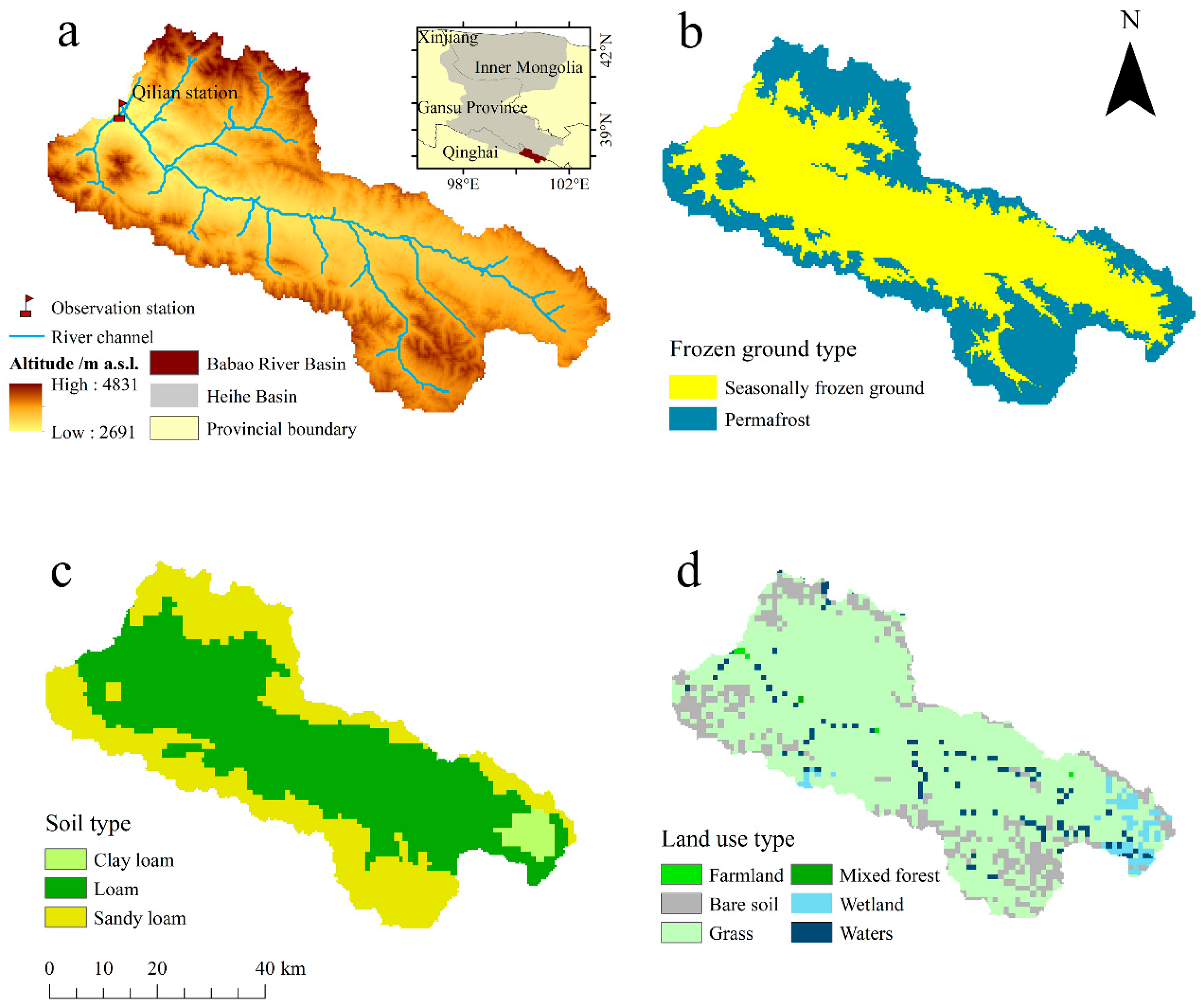
The Babao River, the mainstream in the Babao River Basin, has a total length of about 104.1 km. The basin, located in the Qilian Mountains, Northwest China, has an area of about 2448 km2 and altitudinal variations of more than 2000 m with an average elevation of about 3500 m a.s.l. (Figure 2a). Annual precipitation is about 400 mm and 95% occurs in summer. Primary soil types include clay loam, sandy loam and loam, accounting for 2.5%, 39.5% and 58% of the total basin area, respectively (Figure 2c). The Babao River Basin is a natural basin with few human activities; the primary land cover/use types are grass (78.4%) and bare soil (14.8%). Other types such as water body (3.6%), wetland (2.8%), farmland and mixed forest (0.4%) occupy a small proportion (Figure 2d), and therefore the parameters connected to those types do not attend the sensitivity analysis and calibration. The lower limit of permafrost occurrence is about 3600 m. The SFG exists in lower elevations. According to the map of frozen ground distribution on the Upper Heihe River basin, which fully encloses the Babao River Basin, the permafrost and SFG in the study basin account for 58% and 42% of total areas, respectively (Figure 2b).
The DEM data for the study basin was a subset from the ASTER Global DEM [51], with an original resolution of 30 m. The maps of frozen ground type [52], soil type [53] and land use/cover type [54] reflecting the conditions of around 2010 in the study area were provided by the Cold and Arid Regions Science Data Center at Lanzhou, Northwest China (http://westdc.westgis.ac.cn) and were converted to the grid format. The grid data were then converted to a uniform 300 m model resolution. The observation station, marked Qilian Station in Figure 2a, is located at the outlet of the basin, providing 3 h meteorological records and daily runoff observations. We subset five-year records (2005–2009) to match the other data. The MicroMet approach [55] was employed to interpolate meteorological data into grid cells. MicroMet is an intermediate-complexity, quasi–physically based, meteorological model to produce high-resolution atmospheric data. It is able to provide high-quality meteorological data for mountainous areas by considering topographic impacts to climate variables
The DHSVM version 3.1.2, developed by Pacific Northwest National Laboratory in Seattle, the United States, ran at a time step of 3 h and a spatial resolution of 300 m. Apart from the calibrated parameters, the measurable parameters were assigned with measured values and the rest took the model default values. The river channels in the Babao River Basin were prepared following the approach proposed by Zhao et al. [56]. The runs began with 20 years of spin-up consisting of replicated meteorological records from January 2008 to December 2009. As the DHSVM can output the states at any given time step, the output states on the last 1 October 2008 and 1 May 2009 serve as the initial states of the dry season and wet season, respectively, to the formal runs. The calibration period without season separation is 1 October 2008 to 30 September 2009. The period for dry season calibration is 1 October 2008 to 30 April 2009 and for wet season calibration 1 May 2009 to 30 September 2009. The validation period spans from 1 October 2004 to 30 September 2008, in which 4-year streamflow records are available at the Qilian station.
3. Results
3.1. Sensitive Parameters
Following the workflow in Figure 1, the global sensitivity indices were calculated by eFAST for the nine combinations. Based on the indices, a total of seven sensitive parameters as listed in Table 1 were identified. Among them, three parameters, i.e., monthly albedo (Alb), monthly leaf area index (LAI, m2/m2) and minimum resistance (MinR, s/m), are closely connected to land cover/vegetation, while four of them, i.e., field capacity (FC, m3/m3), lateral conductivity (LC, m/s), bubbling pressure (BP, m) and exponential decrease (ED, m−1) controlling the decay rate of hydraulic conductivity with depth, are associated to soils.
The sensitivity values of those parameters are shown in Table 1, where the sensitivity values are grouped into three levels, i.e., low, medium and high sensitivity, marked by 15%, 20% and 30% grayscale background, respectively. FC, LC and BP have different sensitivity in the permafrost and SFG areas. FC and BP are more sensitive in the permafrost area than the SFG area, whereas LC is more sensitive in the SFG area than permafrost area. Those three parameters influence the simulation of base flow in the DHSVM. By contrast, the land cover/vegetation parameters show stable sensitivity despite the frozen ground type. It also implies no strong correlation exists between parameters associated with the land cover/vegetation type and the frozen ground type.
LAI and MinR are found more sensitive in the wet season than the dry season. They are highly related to surface conditions, affecting overland hydrological processes especially in rainfall periods. The sensitivity of the two soil related parameters, i.e., FC and LC, varies across seasons. However, given soil parameters are usually stable throughout the year, the detected temporal variations in sensitivity are likely induced by the difference of base flow proportion in the total runoff in dry and wet seasons. The base flow proportion presents seasonal variations because the total runoff changes over season, and the absolute volume of base flow, affected by the soil parameters, is maintained at a relatively steady level. According to a previous study [57], LC and FC usually have a strong spatial heterogeneity associated with the spatial distribution of soil intrinsic features (such as density, porosity and permeability) and do not show clear seasonal characteristics. For this reason, Both FC and LC were not considered as season sensitive parameters.
Alb and ED present constant sensitivity in all combinations. Alb is connected to surface conditions that have apparent changes in dry and wet seasons, and it was identified as a season sensitive parameter. Meanwhile, ED is a soil parameter controlling the decay of hydraulic conductivity, which is subject to change in the areas of different frozen ground types. ED was thus considered as a frozen ground type sensitive parameter.
3.2. Calibrated Parametric Values
The optimal values for the sensitive parameters obtained in the four steps are presented in Table 2 and Table 3. Table 2 shows the calibrated values for the parameters relevant to soil types. It is found most parametric values of clay loam are largest and those of loam are smallest among the three soil types. Their values are largely dependent on soil types. Of the same soil type, the values of soil parameters are usually larger in the permafrost area (FroCal/Perm and FullCal/Perm) than in the SFG area (FroCal/SFG and Full/SFG). The differences between frozen ground types imply distinct hydrological characteristics in soils that have different frozen ground types. LC is found insensitive in the permafrost area as well as in the baseline calibration, however, it becomes sensitive when calibrating in the SFG area. FC for the loam is calibrated to take an invariant value of 0.18 across all steps because this value is already the lower boundary able to be assigned to the loam.
Table 3 shows the calibrated values of three seasonally sensitive parameters that are closely related to the land cover type. LAI and MinR appear not sensitive in the dry season (SeaCal/Dry and FullCal/Dry), whereas they become sensitive in the wet season. Alb seems sensitive in both seasons. It has a higher value in the dry season than in wet season in grass-covered areas, and vice versa in bare soils.
3.3. Simulation Results
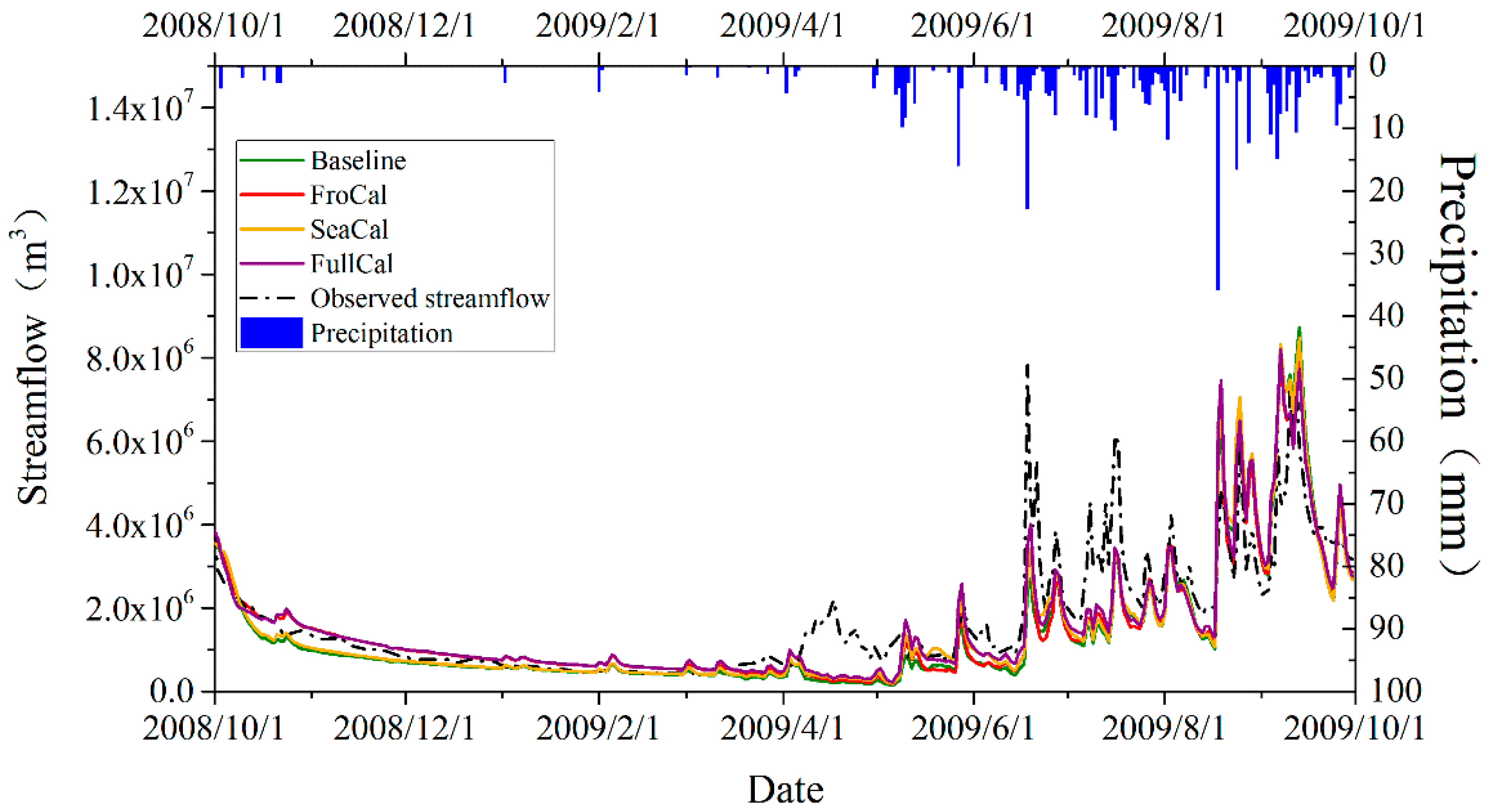
The NSE, KGE and RMSE values measured from the simulated and observed daily streamflow at the Qilian station using calibrated parameters through the four steps of calibrations are presented in Table 4. Compared to the baseline results, all the three metrics show consistently improved performance in the calibration period with the calibrations enforcing spatial or temporal stratifications. The spatially stratifying scheme (FroCal) slightly exceeds the seasonally stratifying scheme (SeaCal) in all stats. The full stratification scheme has the best performance in terms of all metrics. The NSE is increased from 0.58 in the baseline to 0.69 in the full scheme, and the RMSE is reduced from 0.89 × 10⁶ m3 in the baseline to 0.77 × 10⁶ m3 in the full scheme. The daily streamflow time series simulated in the four steps are plotted in Figure 3. It shows overall good agreements of all simulations against the observations, indicating all simulations can capture broader characteristics of streamflow variations. Amidst them, the full scheme has the best simulation whereas the baseline has the worst performance. Meanwhile, all simulations suffer from common weakness such as incapability in reproducing the runoff around April and underestimating some peak flows in summer.
Compared with the results from the baseline and FroCal, the results from SeaCal, in which the model parameters are calibrated by stratifying precipitation seasonality, a present and obvious advantage in the simulation of rainy periods in wet seasons. It improves the NSE and KGE by 0.05 and 0.04, respectively, in comparison with the baseline. It means the adjustment of land cover parameters for separated seasons can enhance the simulation of runoff. While SeaCal occasionally overestimated some peak streamflow in September, it is apparently insufficient in calculating base flow in dry seasons, as suffered in the baseline. By contrast, the FroCal, which considers the frozen ground types in calibration, works much better than the baseline and SeaCal in dry seasons. The baseline and SeaCal results present less base flow in the dry season, which is ameliorated in the FroCal by adjusting soil parameters in stratified areas although slight overestimation still exists compared to the observed. The results with the FullCal (the calibration scheme with full stratification) sharing the joint advantages of FroCal and SeaCal present best consistency with the observed daily streamflow in both trend and magnitude, as indicated by the highest NSE, KGE and lowest RMSE.
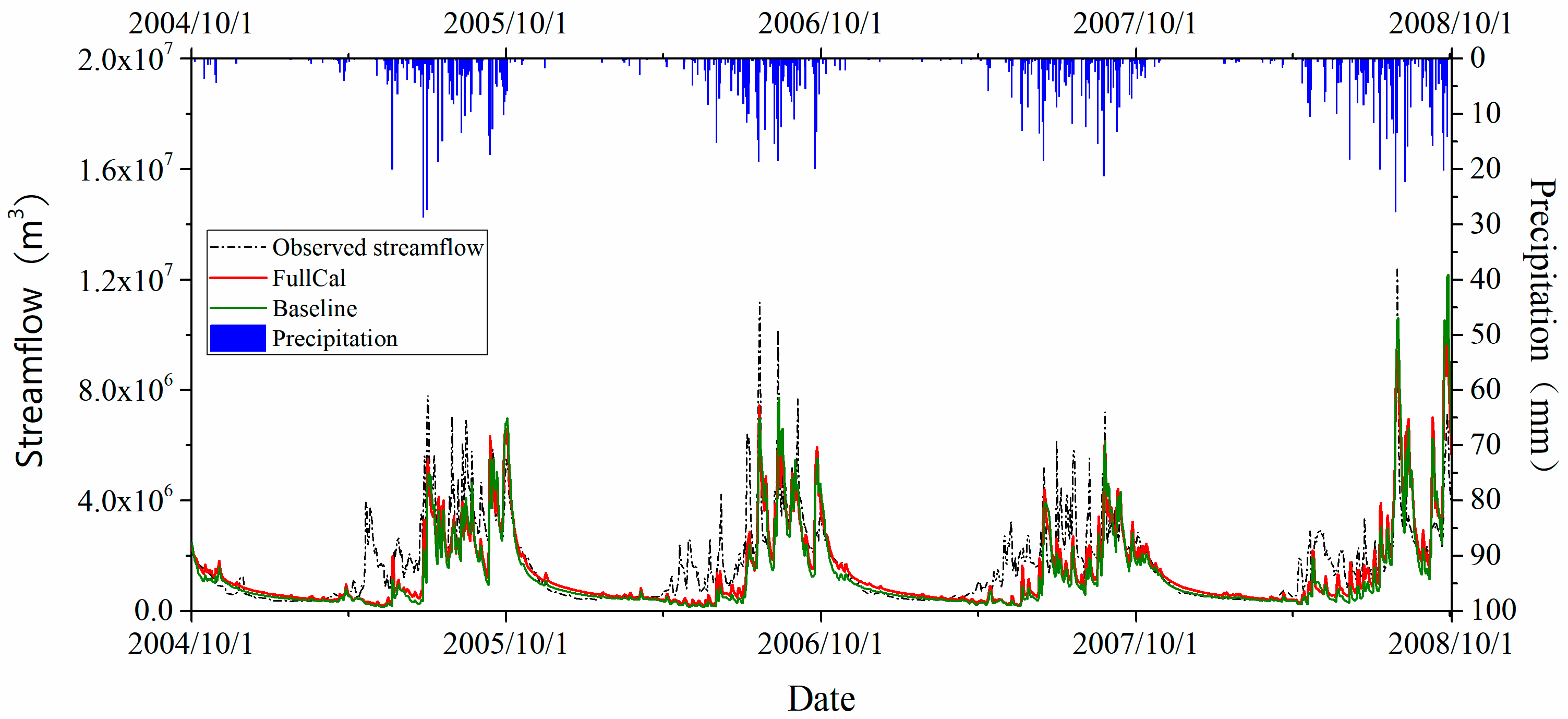
The optimal parameters obtained from the baseline and FullCal were applied to a longer validation period, which lasts four years from 1 October 2004 to 30 September 2008. The time series and stats are displayed in Figure 4 and Table 5, respectively. While all stats become worse to some degree than in the calibration period, the FullCal results keep considerably better than the baseline by 0.12 and 0.08 higher in NSE and KGE, respectively, and by 0.11 × 10⁶ m3 lower in RMSE. The daily streamflow simulated with FullCal has the highest agreement with the observed records in both rainy periods and the periods with scare precipitation. However, both FullCal and baseline have a problem in modeling July and August of 2005 and 2007, when less streamflow has been modelled. The reason is two-folded. On one hand, the DHSVM uses a Penman–Monteith based approach to approximate the actual ET, and the modeling in the Babao River Basin shows overestimation in evaporation and consequent underestimation in the runoff during June to August, the period temperature reaches highest throughout a year. On the other hand, the observed streamflow time series seem to mismatch precipitation at some time and might have some observation errors there.
As exhibited in Figure 3 and Figure 4, the simulations, regardless of any calibration approach employed, consistently fail to reproduce streamflow peaks in around Aprils. It seems only base flow is simulated in those periods. The observed peak streamflow is produced by combinations of thawing active layer of frozen ground, snow melt and glacier melt in early spring when air temperature becomes positive (Figure 5). This proportion of runoff accounted for about 8% of the total annual amount. The DHSVM is capable of simulating snow melt but lacks the model physics of representing freeze and thaw processes occurred within the active layer and glacier melt as well. The calibration experiments help to detect the inadequacy of the model physics.
3.4. Impacts of Frozen Ground Types and Seasons
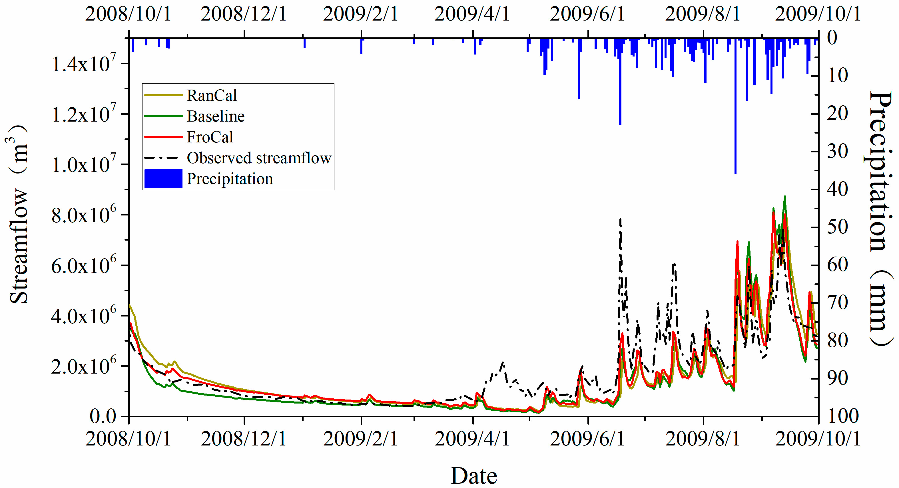
The parametric stratification introduces more parameters, or degrees of freedom, into the model, which mathematically bring more flexibility for calibrating the model. The optimal values for the randomly spatial stratification (RanCal) are listed in Table 6. Comparing to Table 2, where the parameter values in permafrost areas are consistently larger than those in the SFG areas, the changes of parametric values between the two randomly separated areas (R1 and R2 in Table 6) show no obvious patterns. It suggests the stratification into the permafrost and SFG types have significant meaning with respect to model parameters. Figure 6 shows the results from the RanCal, the baseline, and the FroCal that stratifies frozen ground types. Both RanCal and FroCal improve the agreements with the observed daily streamflow especially in the dry season in comparison with the baseline. It confirms the potential effects of the introduction of more parameters into a model. However, the RanCal suffers larger discrepancy in simulating the early recession limb than the FroCal, whereas the latter agrees much better in the same period. The measured NSE, KGE and RMSE of RanCal are 0.61, 0.78 and 0.86 × 10⁶ m3, respectively, while those of FroCal are 0.65, 0.80 and 0.81 × 10⁶ m3, respectively. The increased performance with enforcing a stratified calibration by frozen ground type than the controlled experiment is rooted in the existence of systematic distinction in physiographic characteristics between the permafrost and SFG types.
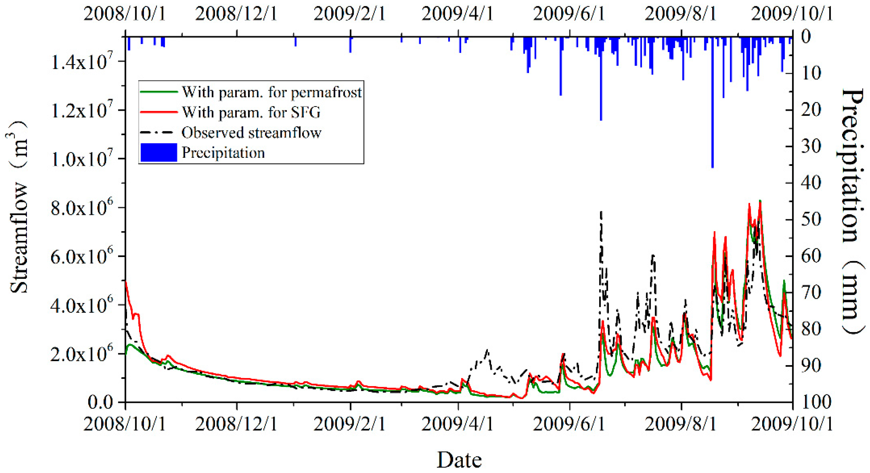
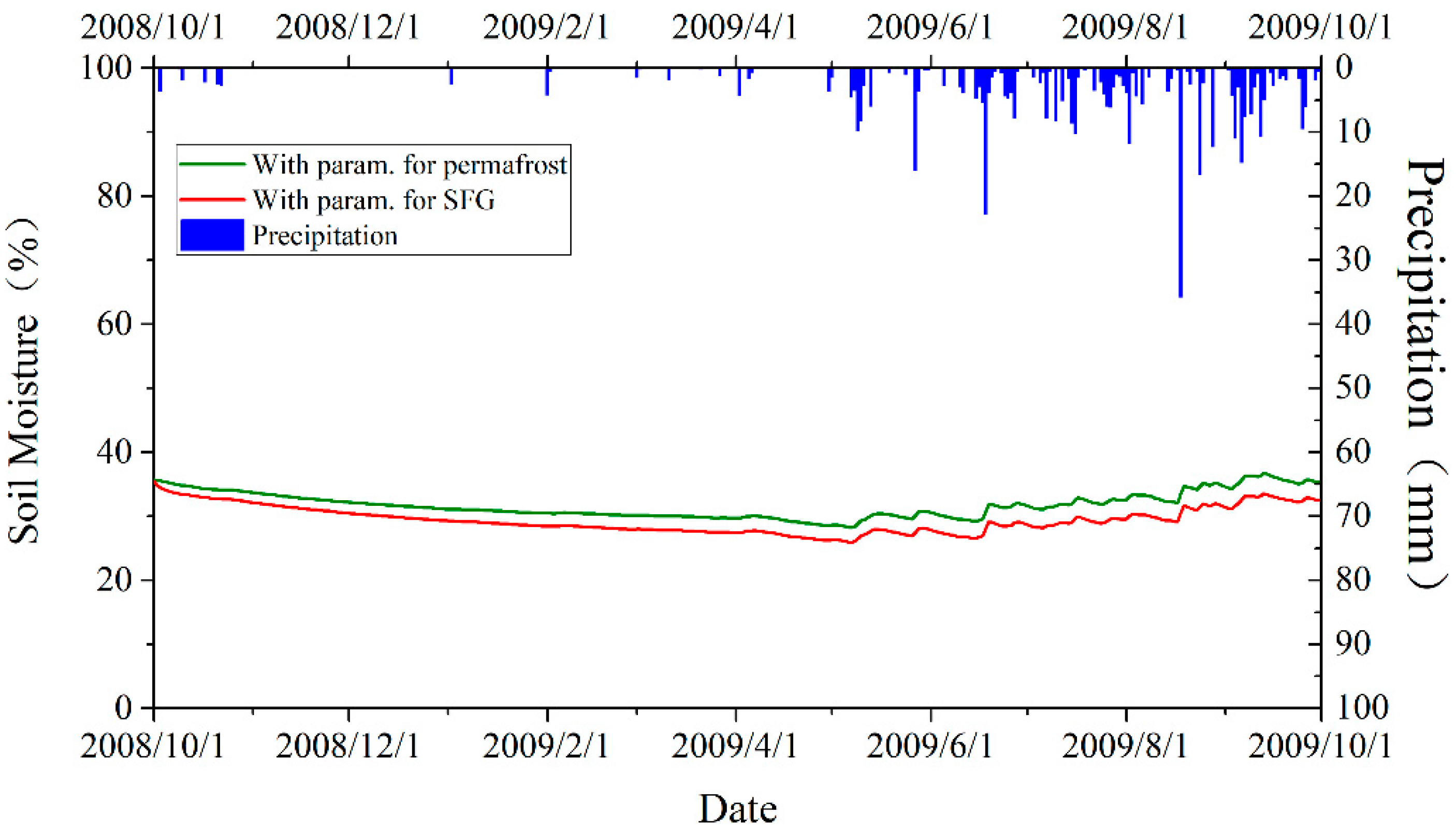
Figure 7 shows the simulated daily streamflow in two hypothetic experiments that applying the parameters for the permafrost area to the entire basin and the parameters for the SFG areas as well, without considering seasonal stratification. The simulated results with the permafrost parameters are less than the SFG parameters in the dry season and low precipitation periods. It is likely caused by more soil moisture content simulated by the permafrost parameters than by the SFG parameters in the whole year (Figure 8) and results in less base flow. Permafrost has lower hydraulic conductivity and higher field capacity than the SFG and holds more soil moisture content in the soil. As less base flow is generated in the permafrost area, the parameter of lateral conductivity (LC) becomes not important and insensitive in modeling the permafrost area (FroCal/Perm and FullCal/Perm) as given in Table 2. Nevertheless, in the SFG area, LC has an effective impact on the generation of base flow. In wet seasons, the results of the two experiments do not differ much but the simulated streamflow with the SFG parameters seems a bit higher than the permafrost parameters but with larger fluctuation. Between the precipitation events, low flows simulated with the permafrost parameters appear more realistic than with the SFG parameters.
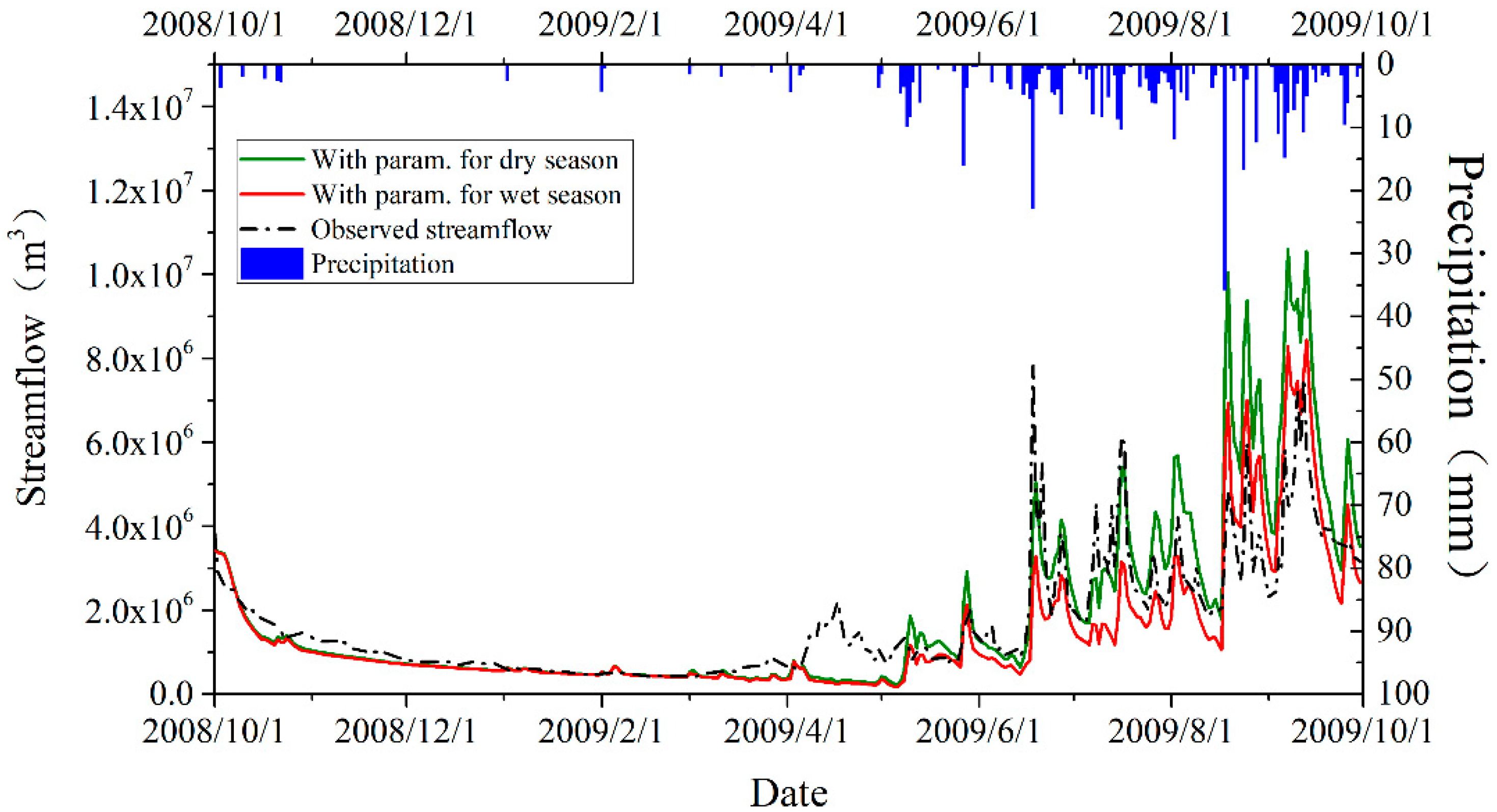
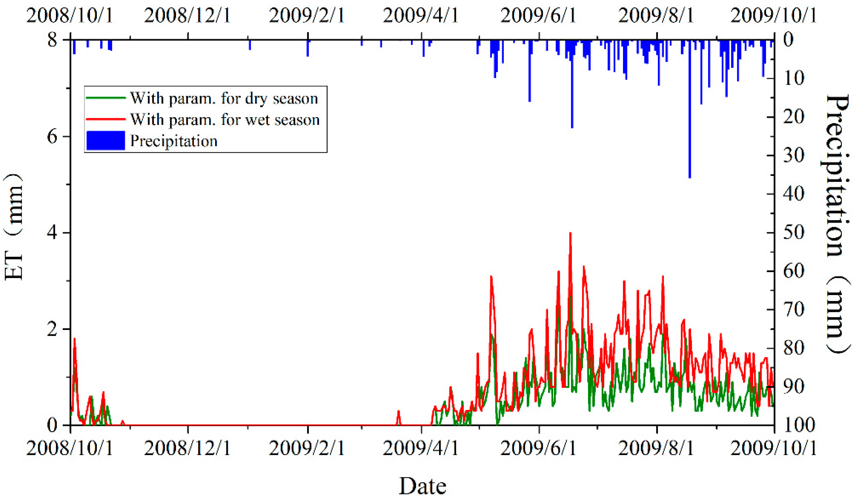
In the hypothetical experiments for the season stratification (Figure 9 and Figure 10), the parameters calibrated for dry seasons lead to less evaporation and more runoff than the parameters for wet seasons do. The two experiments present highly similar simulations in the dry season, both below the measured streamflow. They become distinct from each other in rainfall months. Overall, the parameters for dry seasons result in higher simulated streamflow in rainfall months than those for wet seasons. In June to July, the simulations with the parameters for the dry season approach the observed well while those with the parameters for the wet season tend to underestimate the discharge. In May and August to October, however, the parameters for the wet season work better than the parameters for the dry season. The parameters for dry seasons lead to too much discharge. The reason might be connected to the ET physics in the DHVSM, in which water is excessively evaporated in June to July when using the parameters calibrated for the wet season (Figure 10).
4. Discussion
We identified sensitive parameters in the DHSVM as frozen ground type sensitive and season sensitive parameters when simulating in a cold alpine basin. It shows considerable improvement with calibrated parameters by considering both frozen ground type and season stratification (Figure 3 and Figure 4). Calibrating with stratified frozen ground types will improve the base flow simulation in particular in dry seasons. In permafrost areas, impermeable frozen soil prevents liquid water from passing down and diminishes the downslope outflow. Such effects do not exist in the SFG areas. As revealed in the hypothetical experiments separately testing the permafrost and the SFG parameters in the entire basin (Figure 7 and Figure 8), the optimal parameters for permafrost areas will tend to hold more soil moisture and consequently reduce the base flow. It lays a theoretical basis for necessitating parameter calibration considering spatial stratification by frozen ground type [35,36]. To fully test the advantages of such stratification, it is recommended to purposively set up some discharge gauges in permafrost and SFG dominated sub-catchments. In this study, however, there are no such sub-catchment gauges and we instead validated the results at the final outlet of the study basin. The impacts are positive on the simulation results by stratifying parameters by frozen ground type, especially in dry seasons when the base flow plays a leading role. Meanwhile, calibrating in separated dry and wet seasons is likely to ameliorate the simulation of surface runoff in rainfall periods by mainly adapting the parameters in connection to the land cover types. The Babao River Basin is a natural basin with few human interventions. Grassland in the basin shows strong phenology, therefore, model parameters associated with the vegetation type will change across seasons. Furthermore, because most precipitation concentrates on the wet season, moisture conditions on the land surface also affect the model parameters relevant to land cover type. The joint effects are likely to disable a single set of parameters to represent the real conditions of land cover. The hypothetical experiments (Figure 9 and Figure 10) demonstrate the differences caused by the parameters specific to dry seasons and to wet seasons.
Some existing studies have recognized the importance of temporal stratification in making hydrological model calibration more effective. Zhang et al. [15] calibrated the parameters in the SWAT model by separating dry and wet seasons and reported substantially increased accuracy of simulating daily runoff from an NSE of 0.24 to 0.66 in dry seasons in a cold alpine basin, and from 0.82 to 0.87 in the entire modeling period. However, the results still diverged from the observations in the several dry periods, implying some ill parameterization for the base flow, which is potentially linked to the soil properties of frozen ground underlying the study area. Kim and Lee [34] set up a multiple objective calibration approach by calibrating model parameters in four seasons and found it was insufficient in winter and spring when the superficial soils began freezing or thawing. The R square was found much lower in winter. In a hydrological model, some parameters change substantially over time and can be effectively optimized when considering the seasonal effects to parameters. Some parameters, however, may exhibit notable spatial patterns and can be optimized by purposive spatial stratification. The above-mentioned studies in some way overlook the impacts of different types of frozen ground in a cold alpine basin on the model parameters.
Usually, stratifying the model parameters in space or time will provide more flexibility to the parameter calibration in a hydrological model due to the increase in the number of parameters. While the above-mentioned previous studies have proved the effectiveness of considering stratified seasons, the effectiveness of stratifying frozen ground types for calibration is worthy to investigate. The observed impacts are a mixed result of both increasing numbers of parameters and the real effects of the stratification. The real effects can be identified by a comparative experiment consisting of a calibration scheme with stratified frozen ground type and another one with randomly stratified areas in which only increasing in parameter numbers matters. The results show increasing in parameter numbers is in favor of improving the simulation, although its improvement is less than stratifying frozen ground types. However, we found no apparent pattern in the optimized parametric values from the randomly stratified calibration, which provides little knowledge to understand the real world due to the lack of physics basis. The meaning of parameter calibration is not only to provide a more reasonable combination of parameters but also to study the interaction between the generalized physical processes and parameters [58]. In this sense, a scientifically sound spatial stratification, such as by frozen ground type in a typical cold alpine basin, could well interpret the responses of parameters to different phenomena as well as improve the simulation accuracy and is helpful to promote the understanding of the real world processes. Those physiographical distinctions between the frozen ground types can explain the variability of parameters across frozen ground types.
This study also underlines the importance of complete model physics. Even with a sophisticated calibration approach as presented, it is still impossible to perfectly simulate the streamflow in April. Those defects are related to the occurrence of freeze and thaw processes in the active layer in early spring when the surficial frozen ground begins to melt. Those physics are absent in the adopted version of DHSVM. The stratified calibration scheme could strengthen the impacts of the permafrost and the SFG in a cold alpine basin. They cannot completely replace the physical processes in the model. It urges the need of fitting in place a frozen ground module in the DHSVM to compute the freezing and thawing processes recurring with the oscillating soil temperature. Some efforts have been undertaken in the same basin to enhance the freezing and thawing cycle in models so the simulation in spring has been improved [31]. They suffered notable discrepancy in summer, which can be mitigated by undertaking an appropriate stratified calibration as proposed.
Possible error sources in this study include the quality of data such as meteorological drivers and relatively coarse spatial resolution. The gridded driving forces to DHSVM were interpolated from a single site, the Qilian station, located at the outlet of the Babao River Basin. Although the interpolation method, MicroMet, includes the impacts of topography on climatic variables, the gridded driving forces are subject to uncertainty. In addition, the observed daily streamflow at the Qilian station seems suspicious at some time that abrupt streamflow takes place without matching rainfall. The DHSVM usually requires spatial discretization at a high resolution; the input data in coarse resolutions such as land use/cover and soil maps, which are initially provided at about 1 km resolution, may also come with certain uncertainty to the results in this study.
5. Conclusions
This study proposes a spatially and temporally stratified calibration approach for hydrological modelling in cold alpine basins. This approach takes into account the distinct impacts on model parameters of frozen ground types and precipitation seasonality. A case study applying a distributed hydrological model, DHSVM, in a typical cold alpine basin located in Qilian Mountains, Northwest China, proves the necessity and effectiveness of employing the stratified calibration approach. The following conclusions have been reached:
- The proposed calibration approach by stratifying frozen ground types and seasons could considerably improve the simulation accuracy in cold alpine basins. In the case study, all metrics including the Nash–Sutcliffe coefficient, Kling–Gupta efficiency and root-mean-square error illustrate notable improvements in performance, when the model is calibrated by considering either frozen ground types, seasons, or both. The improvement is substantial when the calibration is stratified by both frozen ground type and season. The improvement keeps significant in a four-year validation period, which is independent of the calibration period.
- The calibration with stratifying frozen ground types is able to effectively adjust base flow in dry seasons and in the periods between precipitation events, while the calibration with stratifying seasons improves in controlling ET and surface flow in rainy periods. In a cold alpine basin where permafrost and the SFG exist, the simulation can be much enhanced by calibrating parameters in stratified frozen ground types. When strong precipitation seasonality is present in the study area, the calibration by considering seasonality will also be in favor of improving the accuracy.
- While the proposed calibration approach leads to better simulation results, it cannot fully compensate for the absence of key physics in the model. Owing to the inadequacy of representing freeze-thaw processes in the active layer in the DHSVM, the simulations cannot correctly reproduce runoffs around April even through the proposed calibration approach. It highlights the importance of improved physics in a hydrological model and the need for complete physics cannot be fully fulfilled by any advanced calibration approach.
Author Contributions
Conceptualization, N.Z., Z.Y. and Y.W.; Methodology, N.Z. and Z.Y.; Software, Z.Y. and Z.L.; Validation, Z.Y.; Formal Analysis, N.Z. and Z.Y.; Resources, N.Z.; Data Curation, Z.Y., Y.W. and Z.L.; Writing—Original Draft Preparation, Z.Y.; Writing—Review and Editing, N.Z.; Supervision, N.Z.; Project Administration, N.Z.; Funding Acquisition, N.Z.
Funding
This study was supported by the grants from National Key R and D Program of China (2017YFA0603603), National Natural Science Foundation of China (41671055), and Natural Science Program of Jiangsu Higher Education Institutions (17KJA170003).
Acknowledgments
This study was also partially supported by Qinglan Talent Program of Nanjing Normal University. The authors thank the Data Management Center of the Heihe Plan for providing data and Pacific Northwest National Laboratory for providing the model.
Conflicts of Interest
The authors declare no conflict of interest.
References
- Moradkhani, H.; Sorooshian, S. General review of rainfall–runoff modeling: model calibration, data assimilation, and uncertainty analysis. Hydrological modeling and the water cycle. In Hydrological Modelling and the Water Cycle: Coupling the Atmospheric and Hydrological Models, 1st ed.; Sorooshian, S., Hsu, K., Coppola, E., Tomassetti, B., Verdecchia, M., Eds.; Springer Science & Business Media: Berlin/Heidelberg, Germany, 2008; pp. 1–24. [Google Scholar]
- Devia, G.K.; Ganasri, B.P.; Dwarakish, G.S. A review on hydrological models. Aquat. Proced. 2015, 4, 1001–1007. [Google Scholar] [CrossRef]
- Gupta, H.V.; Sorooshian, S.; Yapo, P.O. Toward improved calibration of hydrologic models: Multiple and noncommensurable measures of information. Water Resour. Res. 1998, 34, 751–763. [Google Scholar] [CrossRef] [Green Version]
- Morris, M.D. Factorial sampling plans for preliminary computational experiments. Technometrics 1991, 33, 161–174. [Google Scholar] [CrossRef]
- Van Griensven, A.; Meixner, T.; Grunwald, S.; Bishop, T. A global sensitivity analysis tool for the parameters of multi-variable catchment models. J. Hydrol. 2006, 324, 10–23. [Google Scholar] [CrossRef]
- Sobol, I.M. Global sensitivity indices for nonlinear mathematical models and their Monte Carlo estimates. Math. Comput. Simul. 2001, 55, 271–280. [Google Scholar] [CrossRef]
- Saltelli, A.; Tarantola, S.; Chan, K.P.S. A quantitative model-independent method for global sensitivity analysis of model output. Technometrics 1999, 41, 39–56. [Google Scholar] [CrossRef]
- Wang, Q.J. The genetic algorithm and its application to calibrating conceptual rainfall–runoff models. Water Resour. Res. 1991, 27, 2467–2471. [Google Scholar] [CrossRef]
- Duan, Q.Y.; Gupta, V.K.; Sorooshian, S. Shuffled complex evolution approach for effective and efficient global minimization. J. Optimiz. Theory Appl. 1993, 76, 501–521. [Google Scholar] [CrossRef]
- Chu, H.J.; Chang, L.C. Applying particle swarm optimization to parameter estimation of the nonlinear Muskingum model. J. Hydrol. Eng. 2009, 9, 1024–1027. [Google Scholar] [CrossRef]
- Larabi, S.; St-Hilaire, A.; Chebana, F.; Latraverse, M. Multi-criteria process-based calibration using functional data analysis to improve hydrological model realism. Water Resour. Manag. 2018, 32, 195–211. [Google Scholar] [CrossRef]
- Boyle, D.P.; Gupta, H.V.; Sorooshian, S. Toward improved calibration of hydrologic models: Combining the strengths of manual and automatic methods. Water Resour. Res. 2000, 36, 3663–3674. [Google Scholar] [CrossRef]
- Kan, G.; He, X.; Ding, L.; Li, J.; Hong, Y.; Zuo, D.; Ren, M.; Lei, T.; Liang, K. Fast hydrological model calibration based on the heterogeneous parallel computing accelerated shuffled complex evolution method. Eng. Optimiz. 2017, 50, 106–119. [Google Scholar] [CrossRef]
- Wu, Q.; Liu, S.; Cai, Y.; Li, X.; Jiang, Y. Improvement of hydrological model calibration by selecting multiple parameter ranges. Hydrol. Earth Syst. Sci. 2017, 21, 393–407. [Google Scholar] [CrossRef]
- Zhang, D.; Chen, X.; Yao, H.; Lin, B. Improved calibration scheme of SWAT by separating wet and dry seasons. Ecol. Model. 2015, 301, 54–61. [Google Scholar] [CrossRef] [Green Version]
- Madsen, H. Automatic calibration of a conceptual rainfall–runoff model using multiple objectives. J. Hydrol. 2000, 3–4, 276–288. [Google Scholar] [CrossRef]
- Li, Y.; Grimaldi, S.; Pauwels, V.R.N.; Walker, J.P. Hydrologic model calibration using remotely sensed soil moisture and discharge measurements: The impact on predictions at gauged and ungauged locations. J. Hydrol. 2018, 557, 897–909. [Google Scholar] [CrossRef]
- Ha, L.; Bastiaanssen, W.; van Griensven, A.; van Dijk, A.; Senay, G. Calibration of spatially distributed hydrological processes and model parameters in SWAT using remote sensing data and an auto-calibration procedure: A case study in a Vietnamese River basin. Water 2018, 10, 212. [Google Scholar] [CrossRef]
- Cherkauer, K.A.; Lettenmaier, D.P. Hydrologic effects of frozen soils in the upper Mississippi River basin. J. Geophys. Res. Atmos. 1999, 104, 19599–19610. [Google Scholar] [CrossRef] [Green Version]
- Jin, H.; He, R.; Cheng, G.; Wu, Q.; Wang, S.; Lü, L.; Chang, X. Changes in frozen ground in the Source Area of the Yellow River on the Qinghai–Tibet Plateau, China, and their eco-environmental impacts. Environ. Res. Lett. 2009, 4, 045206. [Google Scholar] [CrossRef]
- Niu, G.; Yang, Z. Effects of frozen soil on snowmelt runoff and soil water storage at a continental scale. J. Hydrometeorol. 2006, 7, 937–952. [Google Scholar] [CrossRef]
- Luo, L.; Robock, A.; Vinnikov, K.Y.; Schlosser, C.A.; Slater, A.G.; Boone, A.; Braden, H.; Cox, P.; de Rosnay, P.; Dickinson, R.E.; et al. Effects of frozen soil on soil temperature, spring infiltration, and runoff: Results from the PILPS 2(d) experiment at Valdai, Russia. J. Hydrometeorol. 2003, 4, 334–351. [Google Scholar] [CrossRef]
- Wu, F.; Zhang, J.; Wang, Z.; Zhang, Q. Streamflow variation due to glacier melting and climate change in upstream Heihe River Basin, Northwest China. Phys. Chem. Earth Parts A/B/C 2015, 79–82, 11–19. [Google Scholar] [CrossRef]
- Yao, T.; Thompson, L.; Yang, W.; Yu, W.; Gao, Y.; Guo, X.; Yang, X.; Duan, K.; Zhao, H.; Xu, B.; et al. Different glacier status with atmospheric circulations in Tibetan Plateau and surroundings. Nat. Clim. Chang. 2012, 2, 663–667. [Google Scholar] [CrossRef]
- Zhao, Y.; Nan, Z.; Chen, H.; Li, X.; Jayakumar, R.; Yu, W. Integrated hydrologic modeling in the inland Heihe River Basin, Northwest China. Sci. Cold Arid Reg. 2013, 5, 35–50. [Google Scholar] [CrossRef]
- Kang, E.; Cheng, G.; Lan, Y.; Jin, H. A model for simulating the response of runoff from the mountainous watersheds of inland river basins in the arid area of northwest China to climatic changes. Sci. China Ser. D Earth Sci. 1999, 29, 52–63. [Google Scholar] [CrossRef]
- Chen, R.; Kang, E.; Yang, J.; Zhang, J.; Wang, S. Application of TOPMODEL to simulate runoff from Heihe Mainstream Mountainous Basin. J. Desert Res. 2003, 23, 94–100. [Google Scholar]
- Wang, J.; Li, S. Effect of climatic change on snowmelt runoffs in mountainous regions of inland rivers in northwestern China. Sci. China Ser. D Earth Sci. 2006, 49, 881–888. [Google Scholar] [CrossRef]
- Li, Z.; Xu, Z.; Shao, Q.; Yang, J. Parameter estimation and uncertainty analysis of SWAT model in upper reaches of the Heihe river basin. Hydrol. Process. 2009, 23, 2744–2753. [Google Scholar] [CrossRef]
- Zhang, L.; Jin, X.; He, C.; Zhang, B.; Zhang, X.; Li, J.; Zhao, C.; Tian, J.; DeMarchi, C. Comparison of SWAT and DLBRM for hydrological modeling of a mountainous watershed in arid northwest China. J. Hydrol. Eng. 2016, 21, 4016007. [Google Scholar] [CrossRef]
- Zhang, Y.; Cheng, G.; Li, X.; Jin, H.; Yang, D.; Flerchinger, G.N.; Chang, X.; Bense, V.F.; Han, X.; Liang, J. Influences of frozen ground and climate change on hydrological processes in an alpine watershed: A case study in the upstream area of the Hei’he River, Northwest China. Permafr. Periglac. Process. 2017, 28, 420–432. [Google Scholar] [CrossRef]
- Gao, Y.; Li, K.; Chen, F.; Jiang, Y.; Lu, C. Assessing and improving Noah-MP land model simulations for the central Tibetan Plateau. J. Geophys. Res. Atmos. 2015, 120, 9258–9278. [Google Scholar] [CrossRef]
- Nan, Z.; Shu, L.; Zhao, Y.; Li, X.; Ding, Y. Integrated modeling environment and a preliminary application on the Heihe River Basin, China. Sci. China Technol. Sci. 2011, 54, 2145–2156. [Google Scholar] [CrossRef]
- Kim, H.S.; Lee, S. Assessment of a seasonal calibration technique using multiple objectives in rainfall–runoff analysis. Hydrol. Process. 2014, 4, 2159–2173. [Google Scholar] [CrossRef]
- Kane, D.L.; Stein, J. Water movement into seasonally frozen soils. Water Resour. Res. 1983, 6, 1547–1557. [Google Scholar] [CrossRef]
- Woo, M.K. Permafrost hydrology in North America. Atmos.-Ocean 1986, 3, 201–234. [Google Scholar] [CrossRef]
- Jiang, H.; Zhang, W.; Yi, Y.; Yang, K.; Li, G.; Wang, G. The impacts of soil freeze/thaw dynamics on soil water transfer and spring phenology in the Tibetan Plateau. Arct. Antarct. Alp. Res. 2018, 50, e1439155. [Google Scholar] [CrossRef]
- Woo, M.K.; Marsh, P.; Pomeroy, J.W. Snow, frozen soils and permafrost hydrology in Canada, 1995–1998. Hydrol. Process. 2000, 9, 1591–1611. [Google Scholar] [CrossRef]
- Cuartas, L.A.; Tomasella, J.; Nobre, A.D.; Nobre, C.A.; Hodnett, M.G.; Waterloo, M.J.; Oliveira, S.M.D.; Randow, R.D.C.V.; Trancoso, R.; Ferreira, M. Distributed hydrological modeling of a micro-scale rainforest watershed in Amazonia: Model evaluation and advances in calibration using the new HAND terrain model. J. Hydrol. 2012, 462–463, 15–27. [Google Scholar] [CrossRef]
- Zhao, Q.; Liu, Z.; Ye, B.; Qin, Y.; Wei, Z.; Fang, S. A snowmelt runoff forecasting model coupling WRF and DHSVM. Hydrol. Earth Syst. Sci. 2009, 13, 1897–1906. [Google Scholar] [CrossRef] [Green Version]
- Lan, C.; Lettenmaier, D.P.; Alberti, M.; Richey, J.E. Effects of a century of land cover and climate change on the hydrology of the Puget Sound basin. Hydrol. Process. 2009, 23, 907–933. [Google Scholar] [CrossRef]
- Safeeq, M.; Fares, A. Hydrologic effect of groundwater development in a small mountainous tropical watershed. J. Hydrol. 2012, 428–429, 51–67. [Google Scholar] [CrossRef]
- Lan, C.; Giambelluca, T.W.; Ziegler, A.D.; Nullet, M.A. Use of the distributed hydrology soil vegetation model to study road effects on hydrological processes in Pang Khum Experimental Watershed, Northern Thailand. For. Ecol. Manag. 2006, 224, 81–94. [Google Scholar] [CrossRef]
- Alvarenga, L.A.; de Mello, C.R.; Colombo, A.; Cuartas, L.A.; Bowling, L.C. Assessment of land cover change on the hydrology of a Brazilian headwater watershed using the Distributed Hydrology–Soil–Vegetation Model. Catena 2016, 143, 7–17. [Google Scholar] [CrossRef]
- Wigmosta, M.S.; Vail, L.W.; Lettenmaier, D.P. A distributed hydrology-vegetation model for complex terrain. Water Resour. Res. 1994, 30, 1665–1679. [Google Scholar] [CrossRef]
- Zhao, Y.; Nan, Z.; Li, X.; Xu, Y.; Zhang, L. On applicability of a fully distributed hydrological model in the cold and alpine watershed of Northwest China. J. Glaciol. Geocryol. 2019, 41, 147–157. [Google Scholar]
- Yao, J.; Mao, W.; Yang, Q.; Xu, X.; Liu, Z. Annual actual evapotranspiration in inland river catchments of China based on the Budyko framework. Stoch. Environ. Res. Risk Assess. 2017, 31, 1409–1421. [Google Scholar] [CrossRef]
- Pan, H.; Wang, J.; Li, H. Accuracy validation of the MODIS snow albedo products and estimate of the snow albedo under cloud over the Qilian Mountains. J. Glaciol. Geocryol. 2015, 37, 49–57. [Google Scholar]
- Jiang, M.; Luo, Y.P.; Yang, S.Y. Stochastic convergence analysis and parameter selection of the standard particle swarm optimization algorithm. Inf. Process. Lett. 2007, 102, 8–16. [Google Scholar] [CrossRef]
- Gupta, H.V.; Kling, H.; Yilmaz, K.K.; Martinez, G.F. Decomposition of the mean squared error and NSE performance criteria: Implications for improving hydrological modelling. J. Hydrol. 2009, 377, 80–91. [Google Scholar] [CrossRef] [Green Version]
- Hirano, A.; Welch, R.; Lang, H. Mapping from ASTER stereo image data: DEM validation and accuracy assessment. ISPRS J. Photogramm. Remote Sens. 2003, 57, 356–370. [Google Scholar] [CrossRef]
- Simulation of the Permafrost Distribution over the Upper Reaches of the Heihe River from 1993 to 2012; Heihe Plan Science Data Center: Lanzhou, China, 1993. [CrossRef]
- FAO; IIASA; ISRIC. Harmonized World Soil Database (version 1.1); FAO: Rome, Italy; IIASA: Laxenburg, Austria, 2009. [Google Scholar]
- Ran, Y.; Li, X.; Lu, L.; Li, Z. Large-scale land cover mapping with the integration of multi-source information based on the Dempster–Shafer theory. Int. J. Geograph. Inf. Sci. 2012, 1, 169–191. [Google Scholar] [CrossRef]
- Liston, G.E.; Elder, K. A meteorological distribution system for high-resolution terrestrial modeling (MicroMet). J. Hydrometeorol. 2006, 7, 217–234. [Google Scholar] [CrossRef]
- Zhao, Y.; Cao, X.; Nan, Z.; Wu, X. An automatic method for generating stream network data for the DHSVM model using open source GIS. Remote Sens. Technol. Appl. 2016, 31, 793–800. [Google Scholar]
- Elango, L. Hydraulic Conductivity: Issues, Determination and Applications; InTech: Rijeka, Croatia, 2011; ISBN 978-953-307-288-3. [Google Scholar]
- Klemeš, V. Guest editorial: Of carts and horses in hydrologic modeling. J. Hydrol. Eng. 1997, 2, 43–49. [Google Scholar] [CrossRef]
Figure 1.
Workflow to identify the distributed hydrology–soil–vegetation model (DHSVM) parameters sensitive to frozen ground types and to seasons.
Figure 1.
Workflow to identify the distributed hydrology–soil–vegetation model (DHSVM) parameters sensitive to frozen ground types and to seasons.

Figure 2.
Maps showing the location, (a) topography, (b) frozen ground, (c) soil and (d) land use types in the Babao River Basin.
Figure 2.
Maps showing the location, (a) topography, (b) frozen ground, (c) soil and (d) land use types in the Babao River Basin.

Figure 3.
Simulated daily streamflow with the parameters optimized in each of the four calibrated steps during the calibration period of 1 October 2008 to 30 September 2009.
Figure 3.
Simulated daily streamflow with the parameters optimized in each of the four calibrated steps during the calibration period of 1 October 2008 to 30 September 2009.

Figure 4.
Simulated daily streamflow with the parameters optimized in the baseline and full stratification calibration, respectively, in a four-year validation period (1 October 2004–30 September 2008).
Figure 4.
Simulated daily streamflow with the parameters optimized in the baseline and full stratification calibration, respectively, in a four-year validation period (1 October 2004–30 September 2008).

Figure 5.
Amplified windows of March to May 2005–2009, in which temperature starts to rise across the freezing point, showing incapability of the DHSVM in simulating peak streamflow produced by combinations of thawing active layer of frozen ground, snowmelt and glacier melt.
Figure 5.
Amplified windows of March to May 2005–2009, in which temperature starts to rise across the freezing point, showing incapability of the DHSVM in simulating peak streamflow produced by combinations of thawing active layer of frozen ground, snowmelt and glacier melt.

Figure 6.
Comparison of the effects of spatially stratifying frozen ground type (FroCal) and random spatial stratification (RanCal) on the daily streamflow simulations in the period of 1 October 2008 to 30 September 2009.
Figure 6.
Comparison of the effects of spatially stratifying frozen ground type (FroCal) and random spatial stratification (RanCal) on the daily streamflow simulations in the period of 1 October 2008 to 30 September 2009.

Figure 7.
Simulated daily streamflow with experimentally applying the parameters calibrated for the permafrost area to the entire basin and with the parameters for the seasonally frozen ground (SFG) area.
Figure 7.
Simulated daily streamflow with experimentally applying the parameters calibrated for the permafrost area to the entire basin and with the parameters for the seasonally frozen ground (SFG) area.

Figure 8.
Simulated soil moisture using the parameters calibrated for the permafrost area and for the SFG area.
Figure 8.
Simulated soil moisture using the parameters calibrated for the permafrost area and for the SFG area.

Figure 9.
Simulated daily streamflow with applying the parameters calibrated for dry seasons to the entire year and with the parameters calibrated for wet seasons.
Figure 9.
Simulated daily streamflow with applying the parameters calibrated for dry seasons to the entire year and with the parameters calibrated for wet seasons.

Figure 10.
Simulated evapotranspiration (ET) using the parameters calibrated for dry seasons and for wet seasons, respectively.
Figure 10.
Simulated evapotranspiration (ET) using the parameters calibrated for dry seasons and for wet seasons, respectively.


Table 1.
Sensitivity indices of the DHSVM parameters for each spatial and temporal combination. 15% grayscale represents a sensitivity value of 0.05 to 0.1; 25% 0.1 to 0.2; and 35% >0.2.
Table 1.
Sensitivity indices of the DHSVM parameters for each spatial and temporal combination. 15% grayscale represents a sensitivity value of 0.05 to 0.1; 25% 0.1 to 0.2; and 35% >0.2.
| Category | Parameter | Entire Basin | SFG | Permafrost | ||||||
|---|---|---|---|---|---|---|---|---|---|---|
| Dry | Wet | Both | Dry | Wet | Both | Dry | Wet | Both | ||
| Land cover/vegetation | Monthly albedo (Alb) | 0.12 | 0.10 | 0.09 | 0.12 | 0.13 | 0.11 | 0.12 | 0.10 | 0.09 |
| Monthly LAI (LAI) | - | 0.16 | 0.17 | - | 0.18 | 0.16 | - | 0.16 | 0.18 | |
| Min resistance (MinR) | - | 0.15 | 0.16 | - | 0.10 | 0.13 | - | 0.18 | 0.13 | |
| Soil | Field capacity (FC) | 0.29 | 0.17 | 0.21 | 0.22 | 0.08 | 0.14 | 0.34 | 0.27 | 0.27 |
| Lateral conductivity (LC) | 0.17 | 0.05 | - | 0.26 | 0.06 | 0.06 | 0.08 | - | - | |
| Bubbling pressure (BP) | 0.10 | 0.10 | 0.11 | 0.10 | 0.06 | 0.09 | 0.11 | 0.11 | 0.11 | |
| Exponential decrease (ED) | 0.13 | 0.15 | 0.15 | 0.14 | 0.16 | 0.16 | 0.13 | 0.13 | 0.14 | |
Table 2.
Calibrated values of parameters connected to soil types in four calibration steps. Baseline, FroCal, SeaCal and FullCal stand for calibration Steps 1 to 4, respectively; Perm stands for the permafrost area and SFG the seasonally frozen ground area. SType is short for soil type and Param for parameter. Dash indicates the non-sensitive parameter. Ranges: ED (≥0), BP (>0), FC (wilting point to porosity), LC (>0). The values are round to two decimal places except for LC, which keeps four digits.
| Stype | Param | Baseline | FroCal/SFG | FroCal/Perm | SeaCal | FullCal/SFG | FullCal/Perm |
|---|---|---|---|---|---|---|---|
| Clay Loam | ED | 3.16 | 4.78 | 5.00 | 3.16 | 4.80 | 5.00 |
| BP | 0.36 | 0.69 | 0.76 | 0.36 | 0.69 | 0.76 | |
| FC | 0.33 | 0.18 | 0.27 | 0.33 | 0.18 | 0.27 | |
| LC | - | 0.0070 | - | 0.0210 | 0.0050 | - | |
| Loam | ED | 3.20 | 0.00 | 2.88 | 3.19 | 0.00 | 2.90 |
| BP | 0.29 | 0.10 | 0.76 | 0.29 | 0.10 | 0.76 | |
| FC | 0.18 | 0.18 | 0.18 | 0.18 | 0.18 | 0.18 | |
| LC | - | 0.0002 | - | 0.0008 | 0.0002 | - | |
| Sandy Loam | ED | 2.71 | 2.25 | 4.05 | 2.71 | 2.20 | 4.49 |
| BP | 0.39 | 0.10 | 0.10 | 0.39 | 0.10 | 0.10 | |
| FC | 0.30 | 0.26 | 0.28 | 0.30 | 0.25 | 0.29 | |
| LC | - | 0.1000 | - | 0.0600 | 0.1000 | - |
Table 3.
Calibrated values of land cover relevant parameters in four calibration steps. Baseline, FroCal, SeaCal and FullCal stand for calibration Steps 1 to 4, respectively; Dry is short for the dry season and Wet the wet season. LUType is short for land use type and Param for parameter. Dash indicates the parameter is not sensitive. Ranges: LAI (≥0), MinR (>0), Alb (0–1). The values are round to two decimal places.
| LUType | Param | Baseline | FroCal | SeaCal/Dry | SeaCal/Wet | FullCal/Dry | FullCal/Wet |
|---|---|---|---|---|---|---|---|
| Bare soil | LAI | 1.20 | 1.20 | - | 0.50 | - | 0.50 |
| MinR | 346.17 | 346.17 | - | 300.00 | - | 399.37 | |
| Alb | 0.18 | 0.18 | 0.10 | 0.14 | 0.18 | 0.20 | |
| Grass | LAI | 4.46 | 4.46 | - | 3.12 | - | 2.00 |
| MinR | 389.02 | 389.02 | - | 600.00 | - | 500.00 | |
| Alb | 0.14 | 0.14 | 0.20 | 0.12 | 0.20 | 0.10 |
Table 4.
The Nash–Sutcliffe efficiency (NSE), Kling–Gupta efficiency (KGE) and root-mean-square error (RMSE) measured from the simulated and observed daily streamflow with the parameters optimized in each of the four calibration steps.
Table 4.
The Nash–Sutcliffe efficiency (NSE), Kling–Gupta efficiency (KGE) and root-mean-square error (RMSE) measured from the simulated and observed daily streamflow with the parameters optimized in each of the four calibration steps.
| Calibration Step | NSE | KGE | RMSE (×106 m3) |
|---|---|---|---|
| Baseline | 0.58 | 0.72 | 0.89 |
| FroCal | 0.65 | 0.80 | 0.81 |
| SeaCal | 0.63 | 0.76 | 0.84 |
| FullCal | 0.69 | 0.83 | 0.77 |
Table 5.
The values of Nash–Sutcliffe efficiency (NSE), Kling–Gupta efficiency (KGE) and root-mean-square error (RMSE) of the simulated daily streamflow with the parameters optimized in the baseline and full stratification calibration schemes, respectively, in a four-year validation period (1 October 2004–30 September 2008).
| Calibration Step | NSE | KGE | RMSE (×106 m3) |
|---|---|---|---|
| Baseline | 0.48 | 0.68 | 1.08 |
| FullCal | 0.60 | 0.75 | 0.97 |
Table 6.
Calibrated values of soil-related parameters in the random spatial stratification experiment (RanCal). R1 and R2 represent two randomly separated areas.
Table 6.
Calibrated values of soil-related parameters in the random spatial stratification experiment (RanCal). R1 and R2 represent two randomly separated areas.
| Area | Clay Loam | Loam | Sandy Loam | |||||||||
|---|---|---|---|---|---|---|---|---|---|---|---|---|
| ED | BP | FC | LC | ED | BP | FC | LC | ED | BP | FC | LC | |
| RanCal/R1 | 0.87 | 0.10 | 0.33 | 0.0308 | 2.26 | 0.10 | 0.18 | 0.0012 | 5.00 | 0.10 | 0.25 | 0.0842 |
| RanCal/R2 | 5.00 | 0.25 | 0.32 | - | 3.60 | 0.10 | 0.18 | - | 4.79 | 0.53 | 0.28 | - |
© 2019 by the authors. Licensee MDPI, Basel, Switzerland. This article is an open access article distributed under the terms and conditions of the Creative Commons Attribution (CC BY) license (http://creativecommons.org/licenses/by/4.0/).
Share and Cite
MDPI and ACS Style
Zhao, Y.; Nan, Z.; Yu, W.; Zhang, L. Calibrating a Hydrological Model by Stratifying Frozen Ground Types and Seasons in a Cold Alpine Basin. Water 2019, 11, 985. https://doi.org/10.3390/w11050985
AMA Style
Zhao Y, Nan Z, Yu W, Zhang L. Calibrating a Hydrological Model by Stratifying Frozen Ground Types and Seasons in a Cold Alpine Basin. Water. 2019; 11(5):985. https://doi.org/10.3390/w11050985
Chicago/Turabian StyleZhao, Yi, Zhuotong Nan, Wenjun Yu, and Ling Zhang. 2019. "Calibrating a Hydrological Model by Stratifying Frozen Ground Types and Seasons in a Cold Alpine Basin" Water 11, no. 5: 985. https://doi.org/10.3390/w11050985
Note that from the first issue of 2016, this journal uses article numbers instead of page numbers. See further details here.