Application of Backpack-Mounted Mobile Mapping System and Rainfall–Runoff–Inundation Model for Flash Flood Analysis


1
Disaster Prevention Research Institute, Kyoto University, Gokasho, Uji 611-0011, Japan
2
Graduate School of Engineering, Kyoto University, Nishikyo-ku, Kyoto 615-8540, Japan
3
Leica Geosystems K. K., 1-4-28, Mita, Minato-ku, Tokyo 108-0073, Japan
4
Graduate School of Advanced Integrated Studies in Human Survivability, Kyoto University, Yoshida-Nakaadachi 1, Sakyo-ku, Kyoto 606-8306, Japan
*
Author to whom correspondence should be addressed.
Water 2019, 11(5), 963; https://doi.org/10.3390/w11050963
Submission received: 5 April 2019
/
Revised: 28 April 2019
/
Accepted: 4 May 2019
/
Published: 8 May 2019
(This article belongs to the Special Issue Improving Flood Detection and Monitoring through Remote Sensing)
Abstract
:Satellite remote sensing has been used effectively to estimate flood inundation extents in large river basins. In the case of flash floods in mountainous catchments, however, it is difficult to use remote sensing information. To compensate for this situation, detailed rainfall–runoff and flood inundation models have been utilized. Regardless of the recent technological advances in simulations, there has been a significant lack of data for validating such models, particularly with respect to local flood inundation depths. To estimate flood inundation depths, this study proposes using a backpack-mounted mobile mapping system (MMS) for post-flood surveys. Our case study in Northern Kyushu Island, which was affected by devastating flash floods in July 2017, suggests that the MMS can be used to estimate the inundation depth with an accuracy of 0.14 m. Furthermore, the landform change due to deposition of sediments could be estimated by the MMS survey. By taking into consideration the change of topography, the rainfall–runoff–inundation (RRI) model could reasonably reproduce the flood inundation compared with the MMS measurements. Overall, this study demonstrates the effective application of the MMS and RRI model for flash flood analysis in mountainous river catchments.
1. Introduction
The spatial distribution of inundation depth represents the basic information required to understand the damage of flood disasters. For long-term and large-scale flooding, the use of satellite remote sensing is the most effective way to identify the extent of flood inundations [1,2,3]. Together with topographic data, some methods have been proposed to estimate the dynamics of flood inundation depths [4]. In the case of abrupt, small-scale flooding, such as flash floods in mountainous catchments, it has proven difficult to use satellite remote sensing techniques [5]. To compensate for this situation, detailed rainfall–runoff and flood inundation modeling has been performed to estimate the dynamics of flooding [5,6,7]. Such modeling is essential also for real-time flood forecasting and hazard mapping. Despite considerable advances in modeling, mainly due to the accurate and fine resolution of rainfall and topographic information in recent years, not much technological innovation has occurred in the investigation of high-water marks during post-flood field surveys. In fact, to carry out field measurements of high-water marks with a tape measure is laborious and time-consuming work [8]. Recently, a survey of high-water marks for research purposes was conducted using real-time kinematic GPS (RTK-GPS) [9]. The authors measured the levels of the high-water marks at multiple points for the Kinugawa flooding in the Kanto Region in September 2015 and estimated the spatial distribution of flood inundation depths by spatially interpolating the measurements and subtracting the ground elevation [10]. Since RTK-GPS measures the position of a point and its ground elevation using a single receiver, the measurements can be performed much more easily than in conventional detailed surveying methods. Nevertheless, it is similar to the conventional method in that it repeats the cycle of tasks of moving to the position where the high-water mark is visible, measuring the ground elevation with RTK-GPS, separately measuring the relative height from the ground level to the high-water mark and moving on to the next point. This takes a great deal of time and labor when targeting multiple points over a wide area.
To resolve this problem, the present study examines the application of a mobile mapping system (MMS) in high-water mark surveys. MMS is a surveying instrument consisting of a global navigation satellite system (GNSS), a rapid sequence camera, a laser scanner, and an inertial measurement unit (IMU), as a single package typically mounted on automobiles [11]. More recently, the system is carried in a backpack, which allows us to measure inaccessible sites or the interior of buildings. The MMS provides continuously photographed images and 3D point cloud data (if a laser scanner is embedded), from which we estimate the absolute position of an object, its height, relative length, etc. For application in post-disaster surveys, the Geographical Survey Institute (GSI) of Japan investigated the inundation height of the tsunami caused by the Great East Japan Earthquake using MMS [12]. For river management, the temporal change of riverine topography has been monitored with MMS mounted on a boat or a cart [13,14,15,16,17,18]. For post-flood surveying, however, there have been limited studies applying MMS in high-water mark measurement [9], and its feasibility and effectiveness are not clearly known. If it becomes possible to use MMS for surveys of high-water marks, it will not only enable efficient measurement of high-water marks at multiple points but also serve as a useful disaster record for hazard map creation, as well as verification of flood analysis in future, since this information can be stored as measurable continuous images.
This study applied a backpack-mounted MMS to the post-flood survey of the 2017 northern Kyushu floods. The measured results were compared with the records of direct measurement of high-water marks. In addition, we applied the RRI model [19,20,21] to the same region to simulate the dynamics of flood inundation with and without the effects of topographic change estimated by the MMS. The main objective of the present study is to examine the utility and feasibility of the MMS and RRI model to analyze information on flash flood disasters with the following specific objectives: (1) Investigate the applicability of a backpack-mounted MMS for post-flood surveys; (2) simulate the rainfall–runoff and flood inundation process at the catchment scale by the RRI model; (3) validate the simulation results with local information on the maximum flood inundation depths estimated by the MMS; and (4) discuss the impact of topographic change, also estimated by the MMS, on the flood inundation simulation.
2. Study Sites
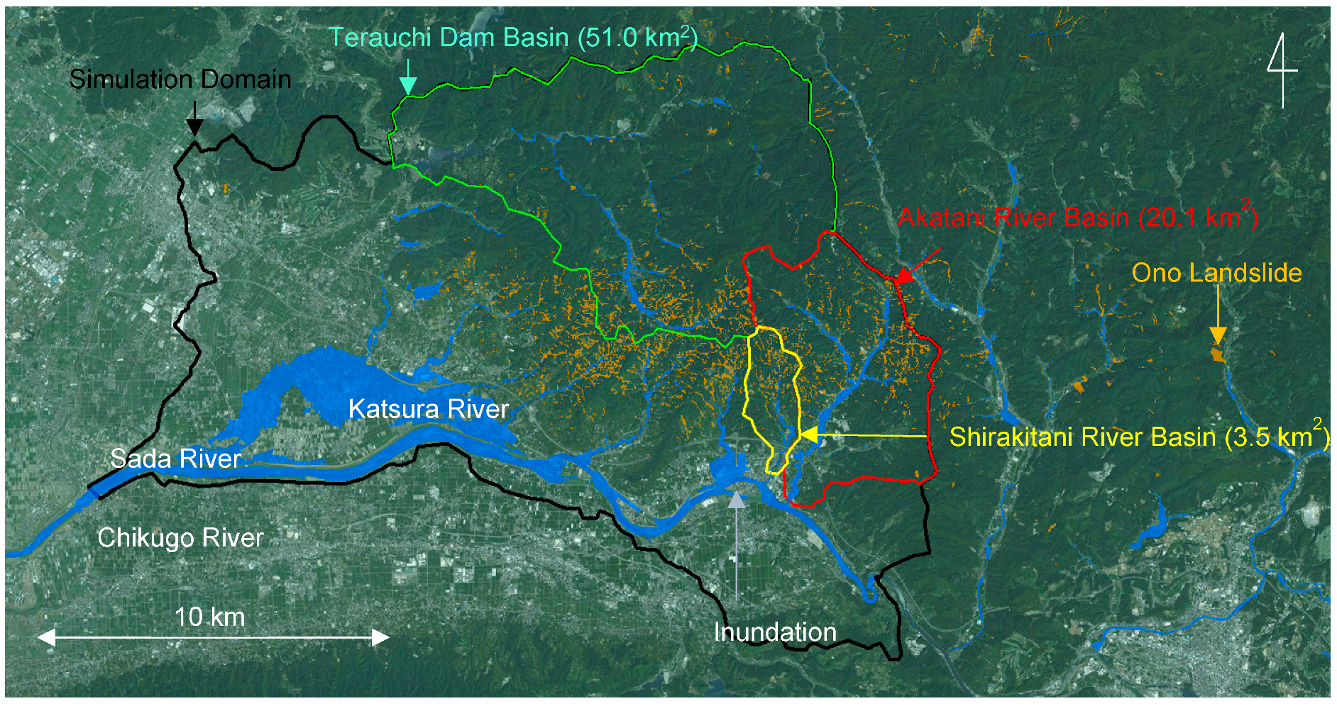
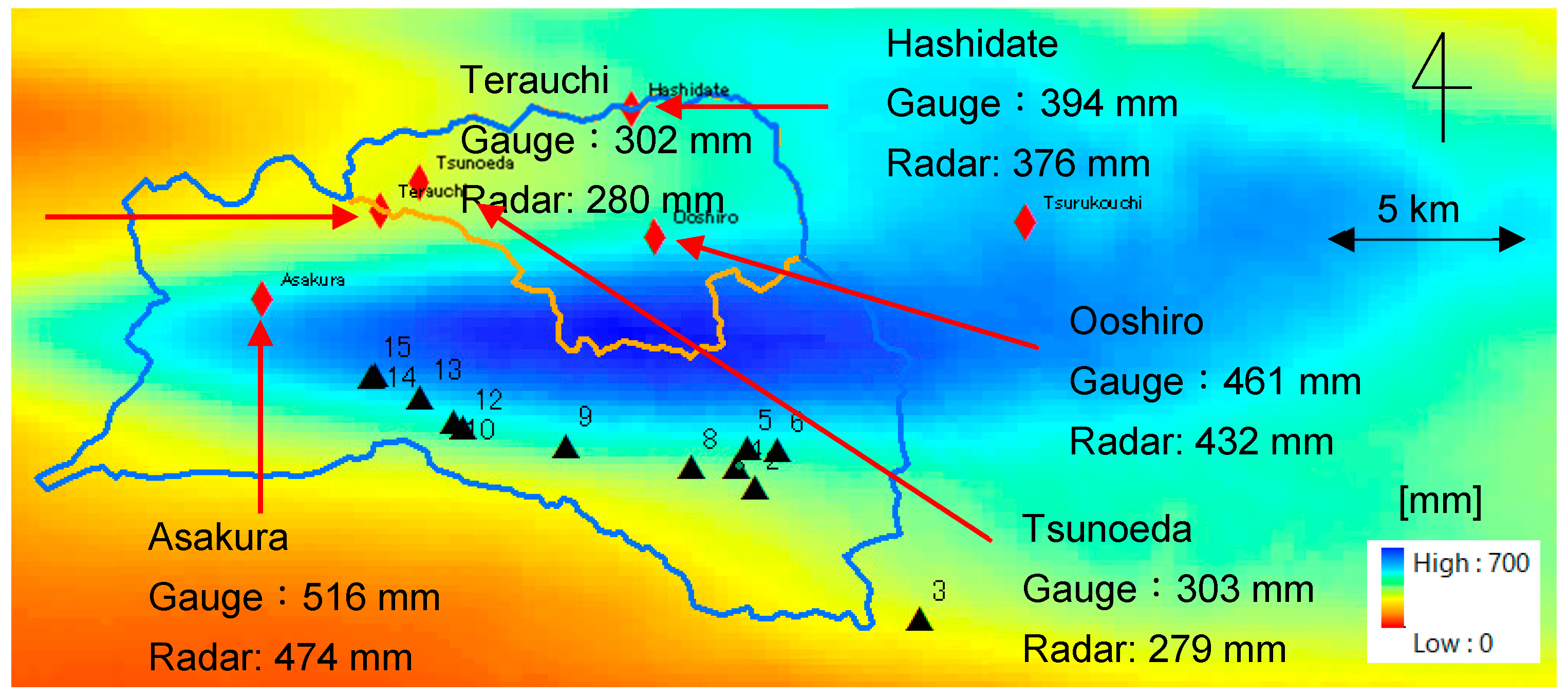
In July 2017, a severe rain band formed over Northern Kyushu Island in Japan induced by a Baiu front and Typhoon No. 3. The rain band brought 829 mm of rainfall within 24 h between July 5, 8:00 and July 6 8:00, while the maximum hourly rainfall was 124 mm (on July 5 14:00–15:00) in Asakura City of Fukuoka Prefecture. The heavy rainfall caused many shallow landslides, which produced massive amounts of sediment and drift wood. The sediment deposits on the floodplains and storm water caused flooding along the tributaries of the Chikugo River (Figure 1). The disasters arising from the flood and sediment killed a total 37 people with 4 people declared missing in Fukuoka and Oita prefectures. Due to the floods, 288 houses were completely collapsed, 1095 and 44 houses were half- or partly-collapsed, respectively, and 172 and 1420 houses were flooded above or below floor levels, respectively.
Figure 2 shows the 24 h accumulated rainfall from midnight on July 5 to midnight on July 6. The rainfall is estimated from the synthetic rainfall products of C-band and X-band radars with 250 m resolution. The distribution of cumulative rainfall extends in an east–west direction, whose range corresponds with the shallow landslides indicated with orange color in Figure 1.
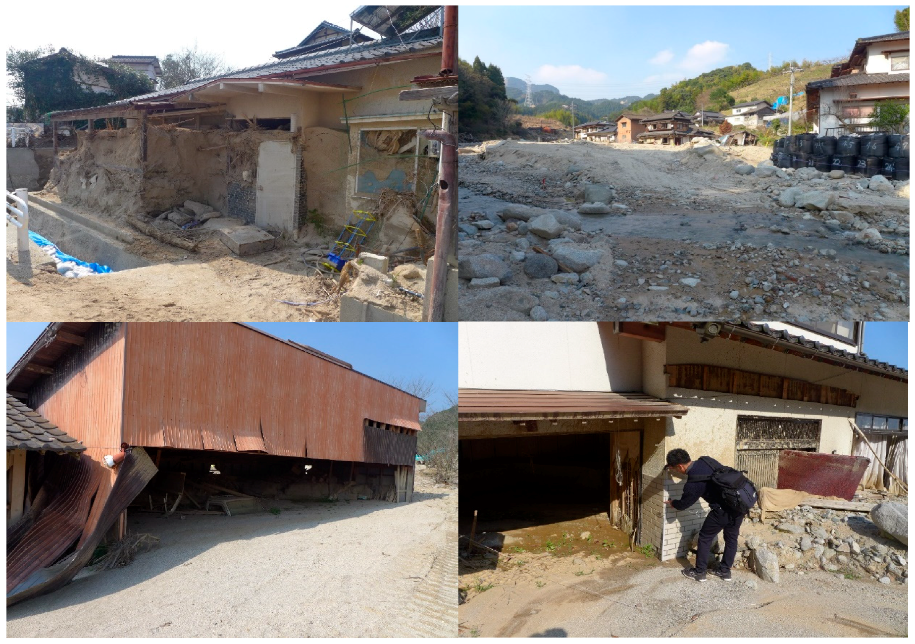
Among the tributaries of the Chikugo River Basin, we selected the Shirakitani River catchment (3.5 km2) for intensive field measurement and simulation, as it was one of the most severely affected river catchments during the storm. The lower part of the Shirakitani River catchment is made up of plutonic granite, while its upper catchment and Western region belong to a metamorphic rock zone derived from mudstone. In the granite area, surface landslides of relatively shallow soil layers had occurred in several places, and as a result, large amounts of sediment and driftwood had buried rivers and riparian terraces (Figure 3).
3. Methods
3.1. Mobile Mapping System (MMS)
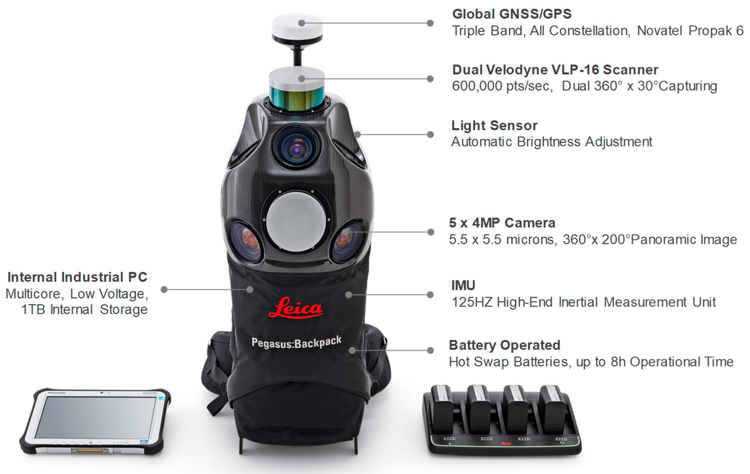
In order to efficiently investigate the state of inundation and topographical changes, a field survey by MMS was carried out. The equipment used is the Leica Pegasus: Backpack (hereafter referred to as PB in this study) [22]. The PB is an MMS system that was conventionally installed in automobiles, now packed in a backpack, and comprises a GNSS, five rapid sequence cameras, two laser scanners, and an IMU (Figure 4). The greatest feature of the PB is its portability, and it is expected to be especially useful for information gathering and field surveys in disaster sites that cannot be accessed by automobiles. Since the weight of the system is about 12 kg, it can be carried as check-in baggage in aircraft and is thus convenient to use in disaster investigations.
The camera mounted on the PB has a charge coupled device (CCD) size of 2046 × 2046, a pixel size of 5.5 μm × 5.5 μm, and a maximum frame rate of 2 frames per second. With five cameras mounted on the sides and in the rear, continuous photographs can be taken at a rear angle of 200°. The laser scanner has a horizontal viewing angle of 270°, a vertical viewing angle of 30°, and a scanning speed of 300,000 points per second. Covering 360° horizontally with two laser scanners, continuous 3-dimensional (3D) data are created by synchronizing the image and 3D point cloud data of the same camera. Further, the installed GNSS supports GPS/Glonass/BeiDu/QZSS. The absolute positioning accuracy has a nominal value of 5 cm outdoors.
3.2. Field Survey with MMS
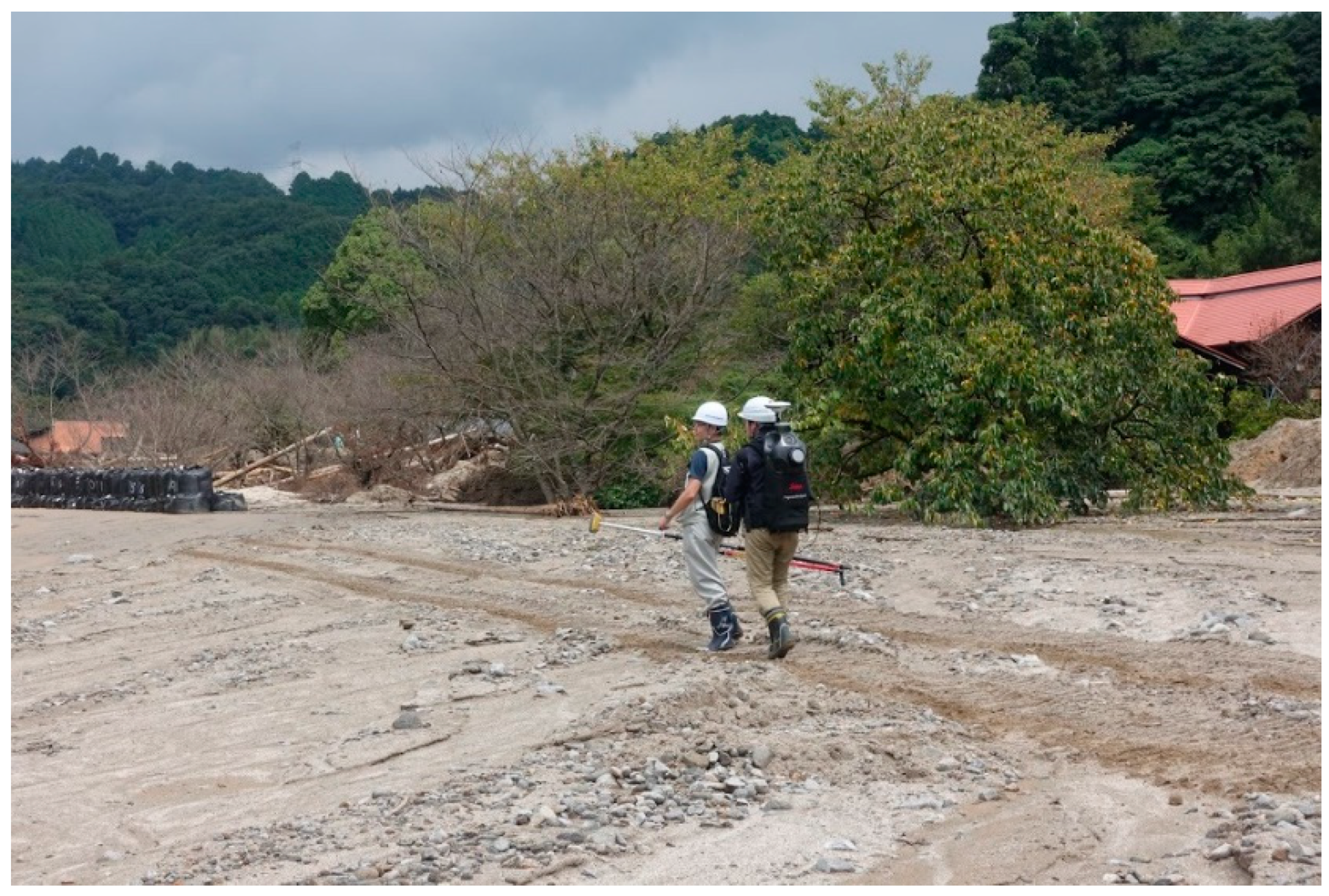
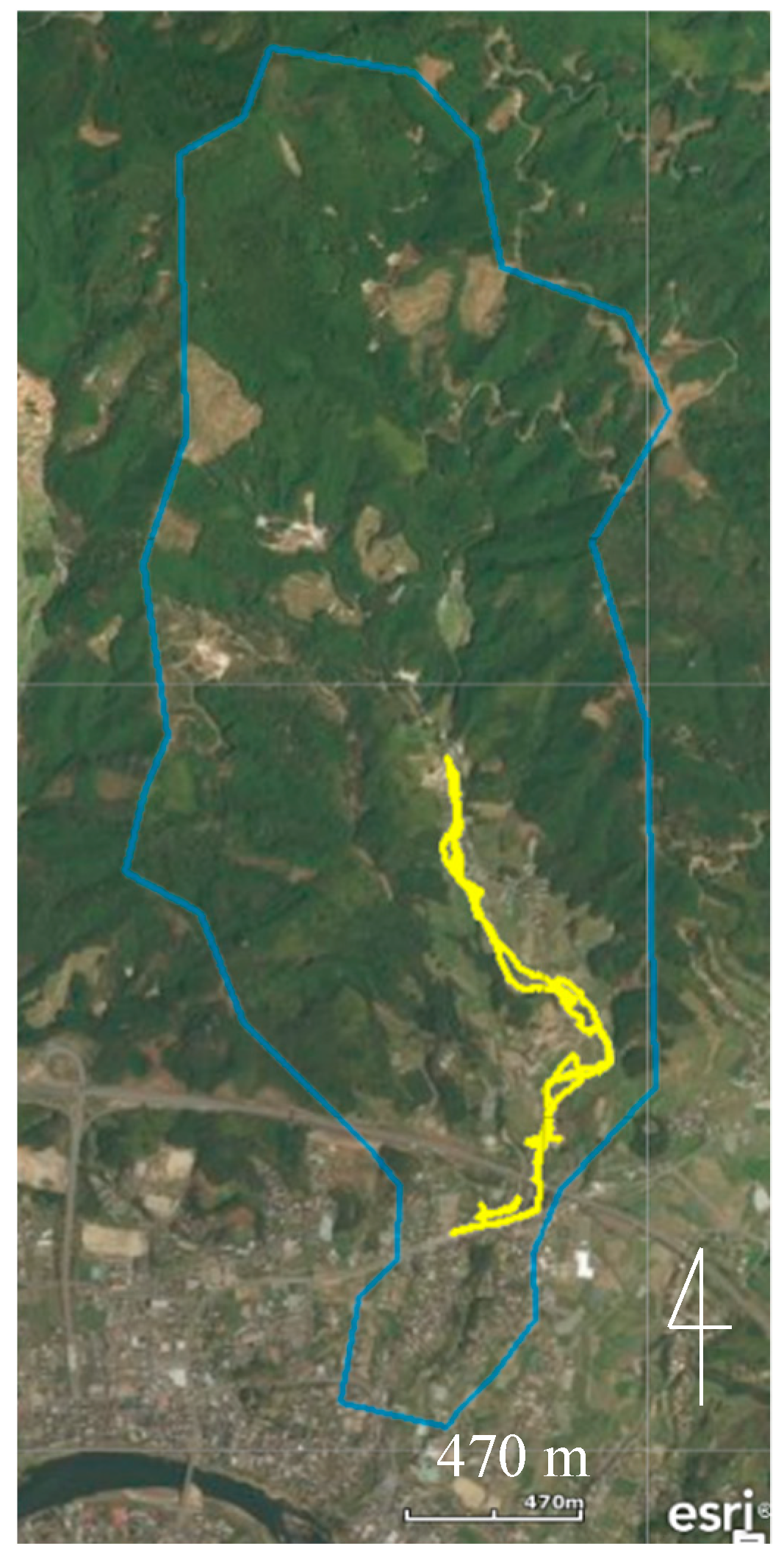
The field survey was conducted on September 12, 2017, and measurements were made by the author along with an engineer from Leica Geosystems (Figure 5). The survey route is indicated by the yellow line in Figure 6, and we made a round trip along the river, covering a distance of about 1.7 km. The time of the actual operation was approximately 3 h. Another survey using RTK-GPS was also conducted in parallel with the PB survey, which required more time than walking normally. In the survey using the PB, however, the investigation could proceed at the same speed as normal walking.
3.3. MMS Data Processing
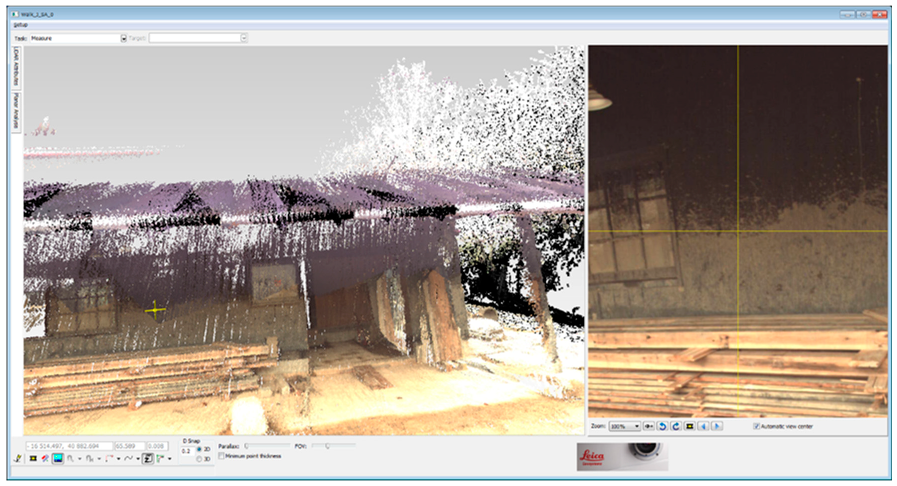
The measured data were synchronized by image processing. The time taken for the image processing also depends on the amount of measurements and took several hours in this case. Once the processing was completed, the captured images can be continuously displayed, and by moving the cursor to a specific location on the screen, the absolute horizontal position and elevation of the object can be measured. In the present case, as we were able to identify high-water marks staining the side walls of buildings, we measured the absolute height of the high-water marks and the inundation depths at 12 points.
In the case of the northern Kyushu disaster, in addition to extracting the level of high-water marks, estimating the topographical change is also important for an understanding of the damage and to carry out the flood analysis, which will be described later. Since the PB creates 3D data for the region around the area covered by walking, analyzing this data will help to estimate the information in relation to the height and surface materials. Furthermore, a digital elevation model (DEM) with a spatial resolution of 10 m and without the influence of buildings and trees was created from the digital surface model (DSM). With the help of this model, it is possible to estimate the terrain after the disaster, and by comparing it with topographical information before the disaster, obtained by an aircraft laser profiler (LP), the depth of sediment deposition could be estimated (Table 1).
3.4. Rainfall–Runoff–Inundation (RRI) Model
This study applied the RRI Model to the Shirakitani River catchment to simulate flooding. The RRI Model is a 2-dimensional (2D) diffusive wave model that takes into account rainfall–runoff and river routing in the rivers and their exchange, representing overtopping flooding (see References [19,20,21] on details of the RRI model). The model treats slopes and river channels separately. For river grid cells, the model supposes that both slope and river are positioned. It applies the 2D diffusive wave model for slope water, while the 1D diffusive wave model is used for channel flow. For better representations of rainfall–runoff–inundation processes, the RRI model simulates also lateral subsurface flow, vertical infiltration flow, and surface flow. In the mountainous regions, the lateral subsurface flow is important. The model uses the discharge–hydraulic gradient relationship, which takes into account both saturated subsurface and surface flows. For flat terrain areas, we assume the vertical infiltration flow is essential and estimated by the Green–Ampt model. The flow interaction between the river channel and slope is estimated based on different overflowing formulae, depending on water-level and levee-height conditions. The model is applied not limited to floodplains but applicable to entire river basins.
The input to the model was the C- and X-band (CX) synthetic radar rainfall and the simulation period was from July 5 0:00 to July 7 0:00. The spatial resolution of the model was set at 10 m, and the model parameters were calibrated during the same period against the observed inflow to the Terauchi Dam (see Figure 1). In this model, the lateral flow and surface flow of the soil layer is reproduced on the mountainous forest slopes. We used two topographic datasets for the simulation, with one based on LP data by GSI, Japan, acquired prior to the disaster, and the other one based on the MMS survey created after the disaster. Although this model can reflect any cross-sectional shape, a simple rectangular cross section has been assumed here on account of the limited information. The width and depth were estimated by the empirical expressions W = CwASw and D = CdASd, respectively. Here, A denotes the area of the catchment (km2) at each location, and Cw, Sw, Cd, and Sd are parameters estimated from the river width and depth at the 8 sites measured in the downstream part of each branch, and set to 4.73, 0.58, 1.57, and 0.33, respectively.
4. Results and Discussions
4.1. Measurement of High-Water Marks by PB
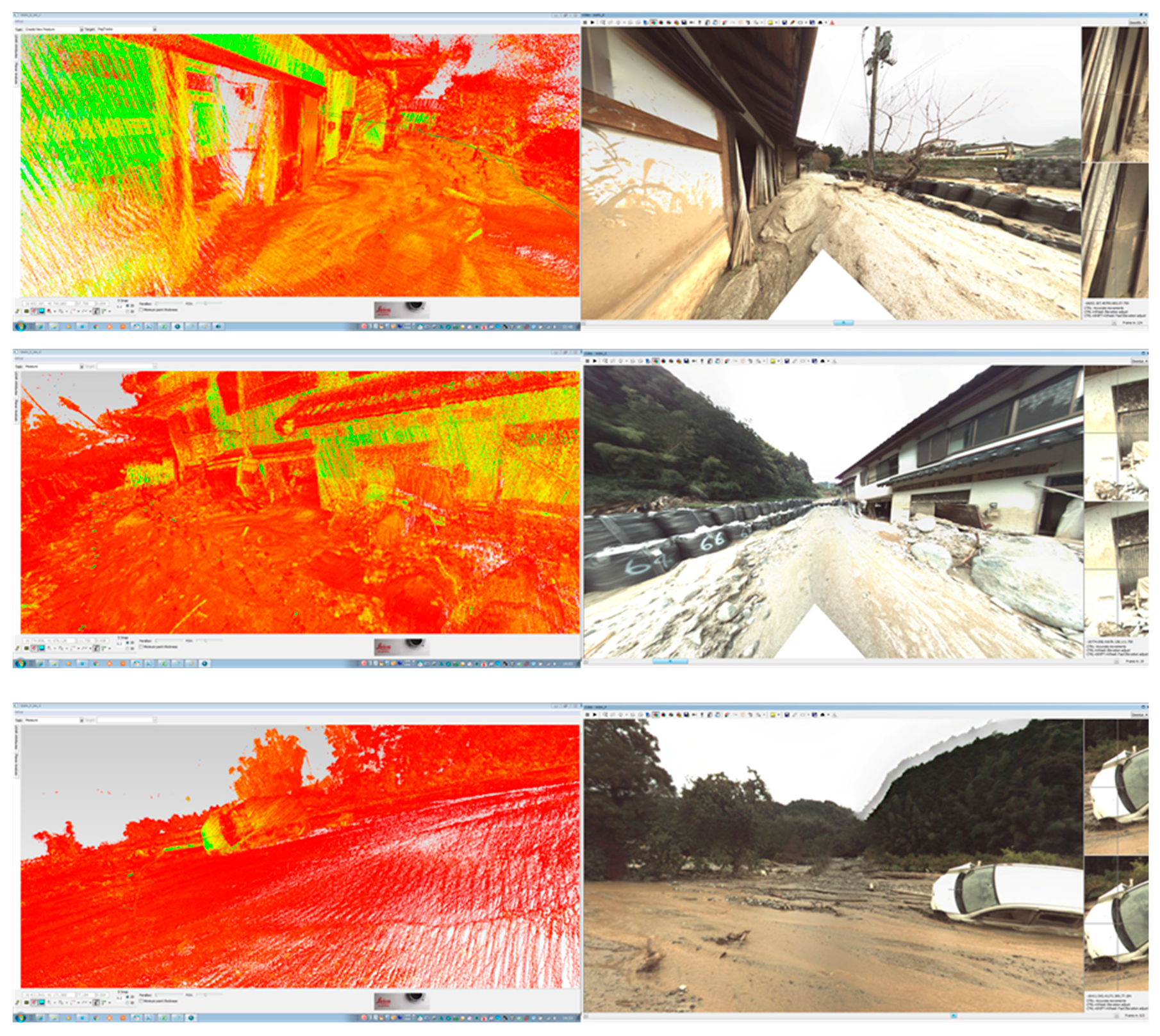
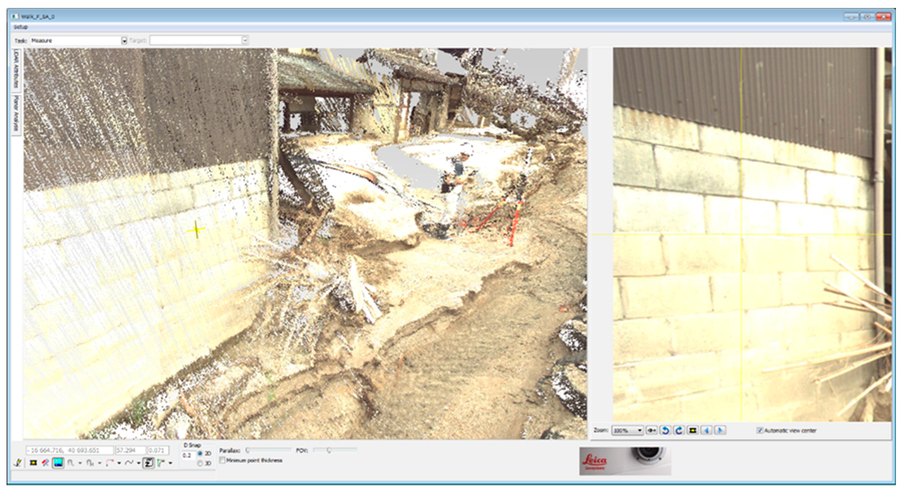
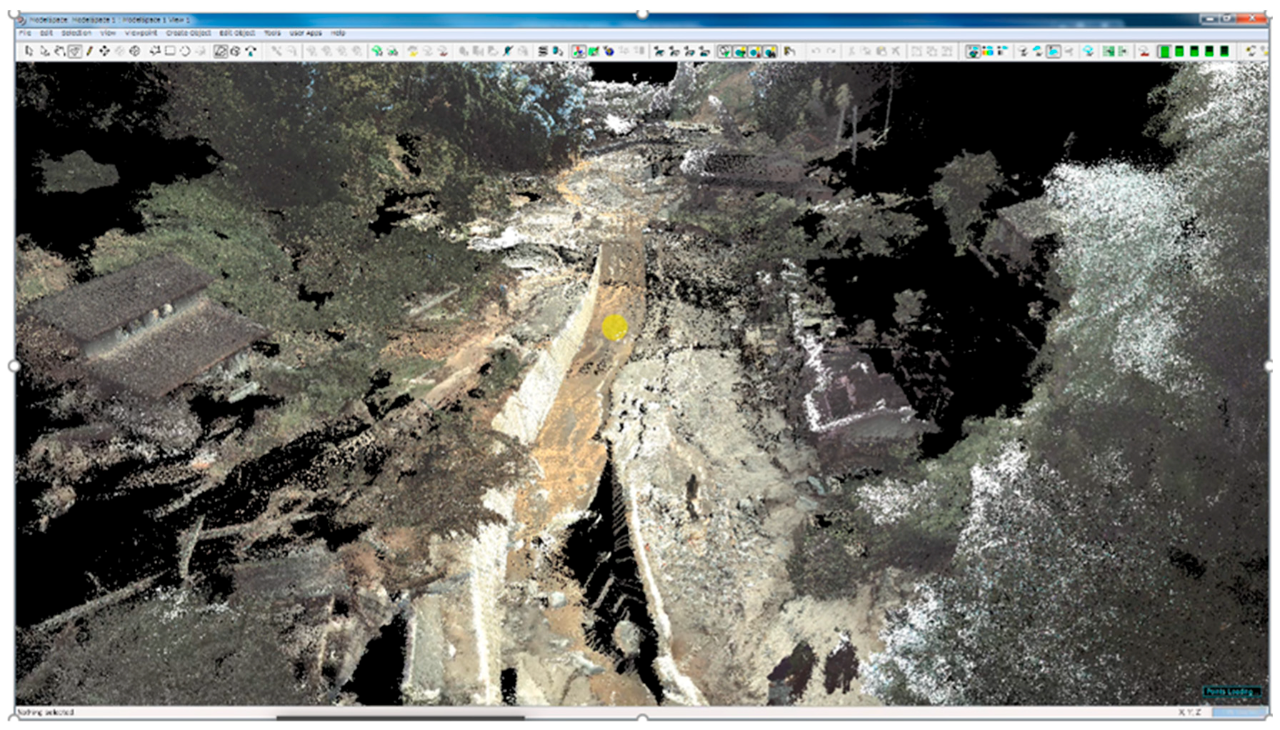
This section presents the results of the field survey with the PB. Figure 7 shows a snapshot of the animation taken by the PB. High-water marks staining houses and fences are visible with adequate clarity in the image. Further, superimposing the color captured by the camera on the 3D point cloud data from the laser yields the images shown in Figure 8 and Figure 9. Being 3D information, it is possible to verify the 3D features, even from angles that are not covered in the actual walking route (Figure 10). The method of displaying the camera image at the center and measuring the high-water mark and ground elevation of the point on the screen was found to be an efficient way to investigate high-water marks.
Table 2 shows the location and inundation depth of high-water marks estimated from the images generated with the PB. The inundation depth estimated from the PB lies in the range of 0.34 m to 1.15 m. It must be noted that this inundation depth was measured from the ground height (G. Level) after the flooding and the raising of the ground level by sediment deposition is not included in this value.
In order to confirm the accuracy of the inundation depth measured using the image, a field survey was conducted once again on March 25, 2018. As shown in Table 2 (Obs: W. Depth), the difference between the PB and field survey was less than 0.11 m, except in the case of two locations, which will be discussed later. As the high-water marks also consisted of water mixed with sediments, there was some uncertainty about which points should be regarded as high-water marks. However, the relative height measurement by the PB was found to have sufficient accuracy with a mean error (ME) of −0.08 and root mean square error (RMSE) of 0.14 m.
The PB values of measurement numbers 9 and 10 are, respectively, 0.25 m and 0.37 m less than the field survey values. In measurement 9, the selection of the measurement site posed a problem, and the splashing of large amounts of deposits mentioned earlier could be responsible for the overestimation of the field measurement. On the other hand, in the case of measurement 10, some of the sediment that accumulated in front of the house had been removed by the time of the survey conducted on March 25, 2018. Since the field measurement measured the depth at a location from where sediment had been removed up to the level of the high-water marks, it is likely to be greater than the inundation depth estimated from the PB image.
Since reference points, such as benchmarks, had not been used in conducting the present survey, it is difficult to discuss, in strict terms, the accuracy of the absolute height estimated by the PB. However, the comparison with the results of the 10 points measured separately using RTK-GPS showed the RMSE in the horizontal direction to be 0.12 m and the RMSE in the vertical direction to be 0.11 m. The accuracy of the RTK-GPS equipment was approximately 0.015 m in the horizontal direction and 0.02 m in the vertical direction. Hence, the PB estimation may be regarded as being sufficiently accurate, considering that it is obtained by simply specifying the target on the screen.
4.2. Estimation of Topographic Changes by PB
A DEM with 10 m spatial resolution was prepared based on the 3D point cloud data measured with the PB. The DEM is limited to a range of about 150 m laterally on either side of the centerline. To create a wide area DEM, it is necessary to carry out longitudinal and lateral surveys. Nevertheless, in creating a DEM of the floodplain along small and medium rivers as in the present case, the range that is generally necessary for exploring along the river was covered.
Figure 11 shows the difference between the topography after the disaster estimated by the PB and by the LP data before the disaster. In much of the measurement range of the PB, the height is observed to rise due to sediment deposition, reaching up to 4 to 5 m in some places in the range of approximately 100 m from the river, where the amount of deposition is particularly high. This is consistent with the scene shown in the photograph in Figure 3 (lower left), where a portion of the house up to the first floor is completely buried under sediments.
4.3. Verification of Rainfall–Runoff–Inundation Simulation with the PB Measurement
We conducted an integrated analysis of rainfall, runoff, and inundation in the Shirakitani River catchment. The inundation depth measurement at multiple points by the PB is useful information for the verification of such flood analysis. Further, the current disaster has resulted in topographical changes due to the massive flow of sediments, and we also discuss here the importance of considering its impact when carrying out flood analysis.
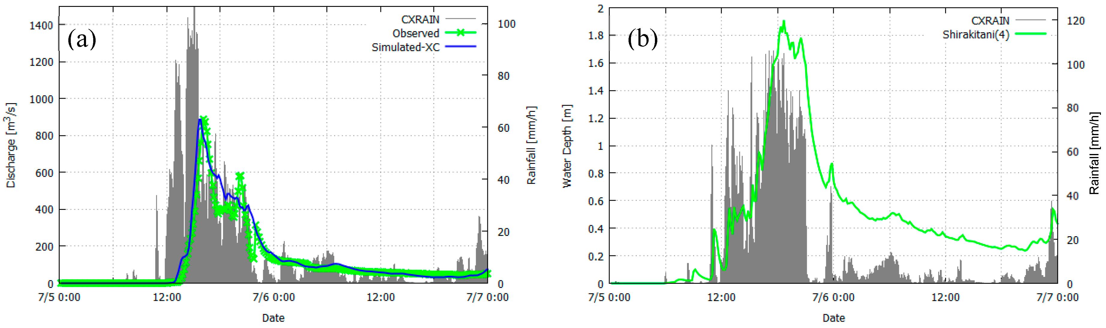
CX synthetic radar rainfall was input to the RRI model to estimate the runoff of the small rivers. The parameters of the model were calibrated with the observed values of the inflow at the Terauchi Dam (Figure 12a). For the present case, the observed dam inflow was well reproduced by setting a relatively thin layer of soil depth (0.6 m) without percolation from the soil layer to the underlying bedrock. Figure 12b shows the estimated hydrograph at the downstream point of Shirakitani River catchment.
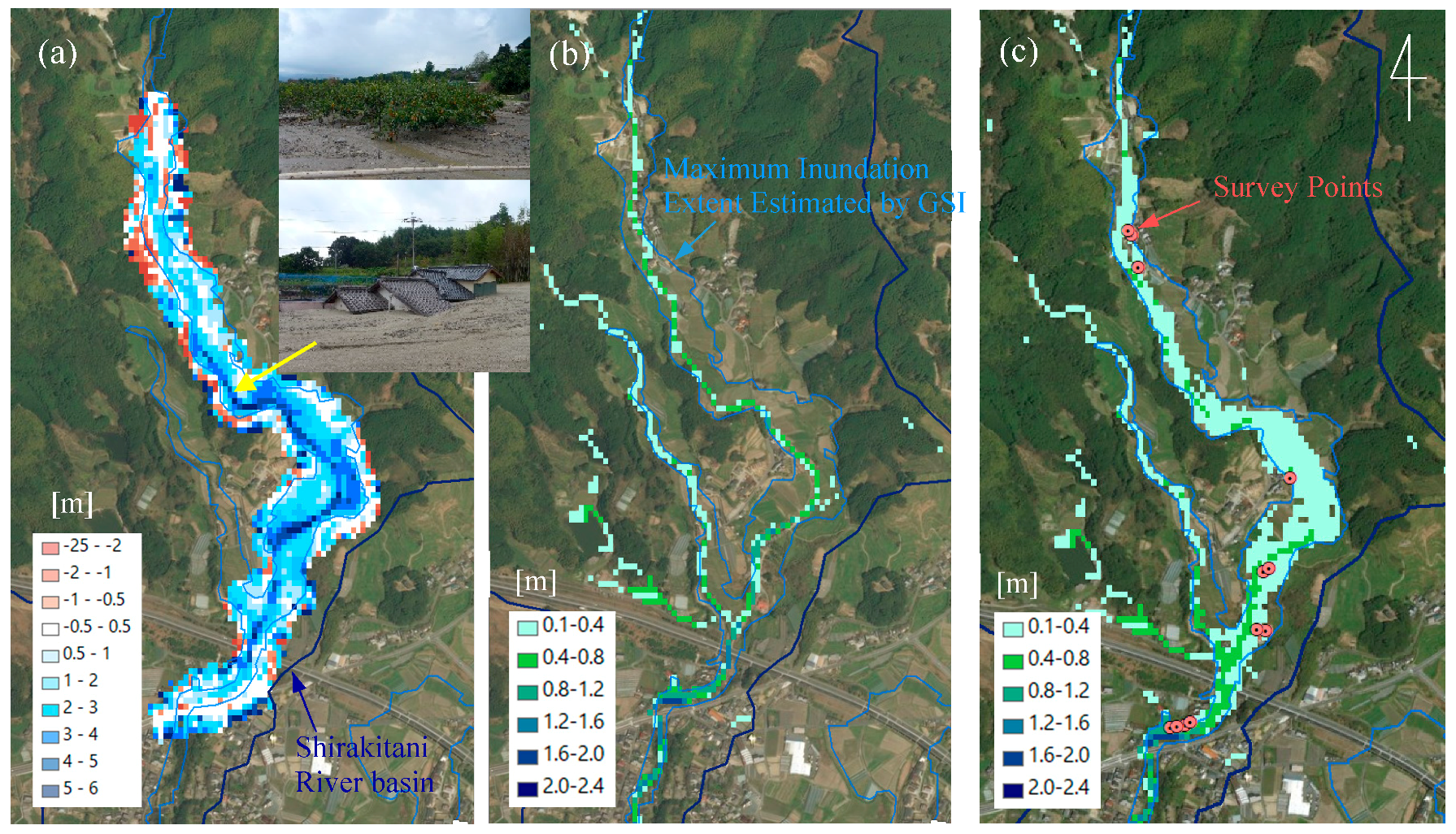
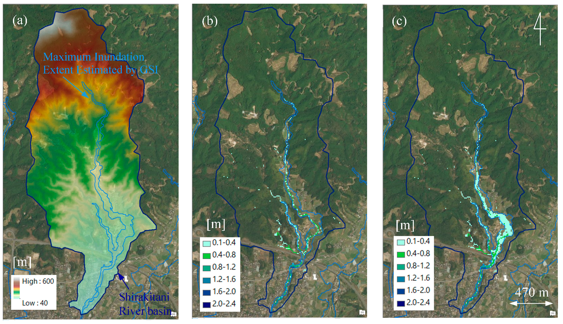
Figure 13b and Figure 14b show the simulated maximum inundation depths in the downstream part and whole catchment, respectively, as estimated by the RRI model. For comparison, we also present the flood inundation extent estimated by GSI, Japan, which determined the maximum flood extent based on aerial photos and field investigation. The comparison suggests that the RRI model underestimates the extent estimated by GSI. This is mainly due to ignorance of the topographic change caused by the sedimentation during the storm event. The maximum water depth is estimated to be about 1.5 m, which only explains the filling of the downstream river channel and does not explain flooding that could fill the floor of the valley, which had actually occurred. This suggests that impediments to the downward flow of the river due to the accumulation of sediments or topographical changes in the flood plains had an impact on the flooding.
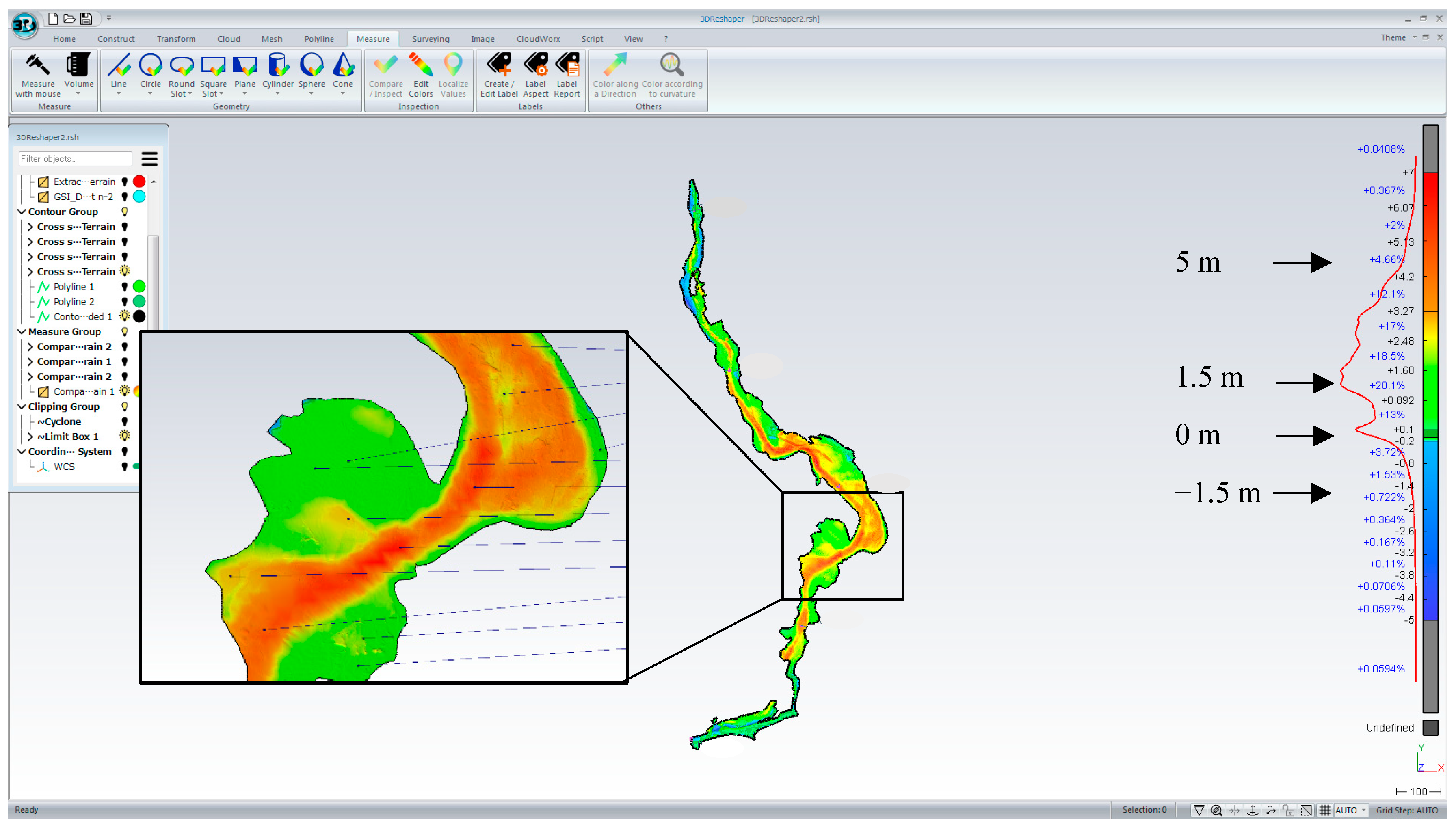
As mentioned earlier, the PB survey provides information about the 3D topography of the surroundings, and hence, the DEM after the disaster can be estimated from the result. Figure 13a shows the amount of topographical change estimated by subtracting the predisaster DEM by the GSI from the DEM estimated by the PB after the disaster. This result is the same as in Figure 11 above but has been obtained by resampling the data with the resolution of 10 m corresponding to the calculation grid of the RRI model. As already mentioned, the analysis result using the DEM before the disaster does not include the inundation of the surroundings (Figure 13b and Figure 14b). The result of the analysis using the topography after the disaster corresponds well with the inundation range given by the GSI, as can be seen in Figure 13c and Figure 14c (blue lines in the figures).
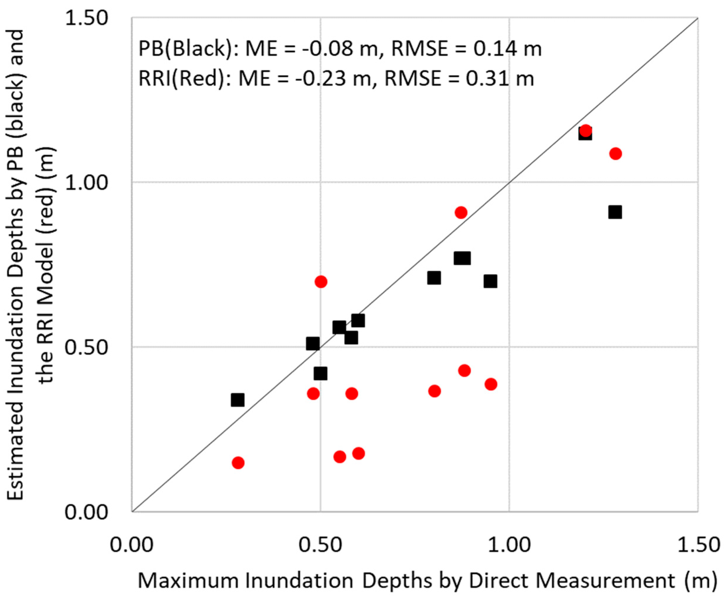
In the graph in Figure 15, the direct measurement of the maximum inundation depth at the 12 points mentioned above have been plotted on the horizontal axis, and the estimation from the PB and RRI models is plotted on the vertical axis. Comparing the field survey and PB values, the mean error (ME) was found to be −0.08 m, and the RMSE was 0.14 m. On the other hand, the comparison between the field survey and the RRI model shows that the ME is −0.23 m and the RMSE is 0.31 m, indicating that the model tends to underestimate the maximum inundation depth. In the analysis, only the rainfall, runoff, and inundation have been calculated based on the topographical changes after the flooding, whereas the outflow and sedimentation contain a mixture of water and sand deposits, which could be the cause of the underestimation.
4.4. On the Potential Use and Limitations of MMS and the Modeling for Post Flood Surveys
Based on the above results, we describe the future prospects for the use of MMS in field surveys immediately after a disaster. In the survey by MMS, since it is possible to concentrate only on collection of images and 3D point cloud data while working at the site, large areas can be investigated quickly compared to the conventional high-water mark surveys that are conducted by stopping at specific places. Moreover, the work is divided into data collection in the field and measurement work at the office, which is a great advantage, especially in surveying disaster areas. Furthermore, since data from MMS can be archived, in addition to becoming a record of the damage, it is particularly useful in verification of the flood analysis as the position and height of any desired place can be measured at any time.
At the start of this research, we had assumed the use of vehicle mounted MMS, but we failed to do so because the disaster-affected area was inaccessible by vehicles. Such vehicle-mounted MMS may be used in wide plain areas. For the disaster affected site here, the backpack type equipment was the most useful alternative. Not all MMSs are equipped with a laser scanning system, and instead, they estimate a relative distance by image processing, which can limit the data size. In the case of having to determine in detail the absolute height of high-water marks, the MMS with a laser scan, such as the PB, is more effective.
Further case studies of the presented approach are definitely required. As described above, the flash flooding in Northern Kyushu Island in July 2017 is characterized with the massive landslides and sedimentation along the floodplain. With high sediment concentration of the inundated water, the visibilities of flood marks may be higher than other cases without sediment concentration. In addition, such a destructive event prevented local residents from immediate recovering activities including clearing flood marks from their houses. These conditions are not necessarily satisfied in other flood events, which may require even rapid post flood surveys.
On the other hand, the sedimentation with the significant topographic changes made it difficult for the flash flood simulation. Due to the current model capability as well as our study scope, we demonstrated the RRI model application with topographic information before and after the disaster event. We suppose this is the first case study using MMS for estimating topographic changes after flash floods in a mountainous region. The MMS survey was inevitable for estimating the topographic change, which was necessary also for the flash flood simulations. Nevertheless, for the better prediction of such disasters, it is important to simulate rainfall–runoff, flood inundation, and sedimentation transportation in a more integrated manner.
5. Conclusions
In this study, we examined the utility and feasibility of using the backpack type MMS (Pegasus: Backpack, PB of Leica Geosystems). We made a 1.7 km long round-trip survey along the Shirakitani River while carrying the equipment and collected continuous images and a 3D point cloud data. Our conclusions are summarized below.
(1) High-water marks due to the flood disaster staining building walls could be clearly identified from the continuous images and 3D point cloud data of the PB. If the level of a high-water mark is specified on the screen, its position and water depth can be measured.
(2) As no special operations are required, except for working with a tablet terminal to make color adjustments to captured images, the survey could proceed at the same speed as walking.
(3) The RMSE of maximum inundation depths measured by the PB was 0.14 m according to the comparison with direct measurements at twelve points. Considering the fact that high-water marks staining the buildings are affected by splashing, the error is thought to be within the permissible range. We believe that the PB has sufficient accuracy to carry out high-water mark measurements.
(4) A new DEM was also created using the PB measurements. It identified a maximum 4 to 5 m of sediment deposits in some places along the river. The information on topographic change was essential for our RRI simulation. The simulation, using the post-disaster topographic data, was found to be closer to the actual flooded area.
(5) The results of the flood analysis by the RRI model were compared with the field survey of inundation depths. The comparison with the field survey showed an ME of −0.23 m and RMSE of 0.31 m, indicating that the model tended to slightly underestimate the maximum inundation depth. In the analysis, only the rainfall runoff and inundation have been calculated based on the topographical changes after the flooding, whereas in reality, the outflow and sedimentation contain a mixture of water and sand deposits, which may have affected the results of the analysis.
Overall, this study demonstrated the high potential of the wearable MMS and the RRI model in post-flood analysis. Survey-related technologies, such as MMS and drones, have been making impressive advances, and it is important to gather and archive information about disaster-affected areas utilizing such state-of-the-art technology.
Author Contributions
Conceptualization, T.S.; methodology, T.S. and Y.K.; software, Y.K.; validation, T.S., K.M.; formal analysis, T.S.; investigation, T.S.; resources, K.T.; data curation, K.M.; writing—original draft preparation, T.S.; writing—review and editing, T.S.; visualization, T.S., K.M. and Y.K.; supervision, K.T.; project administration, T.S.; funding acquisition, T.S. and K.T.
Funding
This study was supported by the River Fund of The River Foundation, Japan, JSPS KAKENHI Grant Number 15H04051 (PI: T. Sayama) and JSPS Grant-in-Aid for Special Purposes 17K20140 (PI: J. Akiyama).
Acknowledgments
We acknowledge the technical support by Leica Geosystems K. K., Japan for the technical support of Pegasus: Backpack.
Conflicts of Interest
The authors declare no conflict of interest.
References
- Schumann, G.; Bates, P.D.; Horritt, M.S.; Matgen, P.; Pappenberger, F. Progress in integration of remote sensing–derived flood extent and stage data and hydraulic models. Rev. Geophys. 2009, 47. [Google Scholar] [CrossRef] [Green Version]
- Bates, P.D. Integrating remote sensing data with flood inundation models: How far have we got? Hydrol. Process. 2012, 26, 2515–2521. [Google Scholar] [CrossRef]
- Rahman, M.S.; Di, L. The state of the art of spaceborne remote sensing in flood management. Nat. Hazards 2016, 85, 1223–1248. [Google Scholar] [CrossRef]
- Nguyen, N.Y.; Ichikawa, Y.; Ishidaira, H. Estimation of inundation depth using flood extent information and hydrodynamic simulations. Hydrol. Res. Lett. 2016, 10, 39–44. [Google Scholar] [CrossRef]
- Elfeki, A.; Masoud, M.; Niyazi, B. Integrated rainfall–runoff and flood inundation modeling for flash flood risk assessment under data scarcity in arid regions: Wadi Fatimah basin case study, Saudi Arabia. Nat. Hazards 2016, 85, 87–109. [Google Scholar] [CrossRef]
- Kvočka, D.A.; Ahmadian, R.; Falconer, R. Flood Inundation Modelling of Flash Floods in Steep River Basins and Catchments. Water 2017, 9, 705. [Google Scholar] [CrossRef]
- Mashaly, J.; Ghoneim, E. Flash Flood Hazard Using Optical, Radar, and Stereo-Pair Derived DEM: Eastern Desert, Egypt. Remote Sens. 2018, 10, 1204. [Google Scholar] [CrossRef]
- Koenig, T.A.; Bruce, J.L.; O’Connor, J.E.; McGee, B.D.; Holmes, R.R., Jr.; Hollins, R.; Forbes, B.T.; Kohn, M.S.; Schellekens, M.F.; Martin, Z.W.; et al. Identifying and Preserving High-Water Mark Data; U.S. Geological Survey: Reston, VA, USA, 2016; 47p.
- Meesuk, V.; Vojinovic, Z.; Mynett, A.E. Extracting inundation patterns from flood watermarks with remote sensing SfM technique to enhance urban flood simulation: The case of Ayutthaya, Thailand. Comput. Environ. Urban Syst. 2017, 64, 239–253. [Google Scholar] [CrossRef]
- Sayama, T.; Takara, K. Estimation of Inundation Depth Distribution for the Kinu River Flooding by 2015.09 Kanto-Tohoku Heavy Rainfall. J. Jpn. Soc. Civ. Eng. Ser. B1 (Hydraul. Eng.) 2016, 72, I_1171–I_1176. [Google Scholar] [CrossRef]
- Lauterbach, H.A.; Borrmann, D.; Hess, R.; Eck, D.; Schilling, K.; Nuchter, A. Evaluation of a Backpack-Mounted 3D Mobile Scanning System. Remote Sens. 2015, 7, 13753–13781. [Google Scholar] [CrossRef] [Green Version]
- Koarai, M.; Okatani, T.; Nakano, T.; Nakamura, T.; Hasegawa, M. Geographical Information Analysis of Tsunami Flooded Area by the Great East Japan Earthquake Using Mobile Mapping System. Int. Arch. Photogramm. 2012, 39-B8, 27–32. [Google Scholar] [CrossRef]
- Vaaja, M.; Hyyppa, J.; Kukko, A.; Kaartinen, H.; Hyyppa, H.; Alho, P. Mapping Topography Changes and Elevation Accuracies Using a Mobile Laser Scanner. Remote Sens. 2011, 3, 587–600. [Google Scholar] [CrossRef] [Green Version]
- Saarinen, N.; Vastaranta, M.; Vaaja, M.; Lotsari, E.; Jaakkola, A.; Kukko, A.; Kaartinen, H.; Holopainen, M.; Hyyppa, H.; Alho, P. Area-Based Approach for Mapping and Monitoring Riverine Vegetation Using Mobile Laser Scanning. Remote Sens. 2013, 5, 5285–5303. [Google Scholar] [CrossRef] [Green Version]
- Williams, R.D.; Brasington, J.; Vericat, D.; Hicks, D.M. Hyperscale terrain modelling of braided rivers: fusing mobile terrestrial laser scanning and optical bathymetric mapping. Earth Surf. Proc. Landf. 2014, 39, 167–183. [Google Scholar] [CrossRef]
- Leyland, J.; Hackney, C.R.; Darby, S.E.; Parsons, D.R.; Best, J.L.; Nicholas, A.P.; Aalto, R.; Lague, D. Extreme flood-driven fluvial bank erosion and sediment loads: Direct process measurements using integrated Mobile Laser Scanning (MLS) and hydro-acoustic techniques. Earth Surf. Proc. Landf. 2017, 42, 334–346. [Google Scholar] [CrossRef]
- Entwistle, N.; Heritage, G.; Milan, D. Recent remote sensing applications for hydro and morphodynamic monitoring and modelling. Earth Surf. Proc. Landf. 2018, 43, 2283–2291. [Google Scholar] [CrossRef]
- Lotsari, E.S.; Calle, M.; Benito, G.; Kukko, A.; Kaartinen, H.; Hyyppä, J.; Hyyppä, H.; Alho, P. Topographical change caused by moderate and small floods in a gravel bed ephemeral river—A depth-averaged morphodynamic simulation approach. Earth Surf. Dyn. 2018, 6, 163–185. [Google Scholar] [CrossRef]
- Sayama, T.; Ozawa, G.; Kawakami, T.; Nabesaka, S.; Fukami, K. Rainfall–runoff–inundation analysis of the 2010 Pakistan flood in the Kabul River basin. Hydrol. Sci. J. 2012, 57, 298–312. [Google Scholar] [CrossRef] [Green Version]
- Sayama, T.; Tatebe, Y.; Tanaka, S. An emergency response-type rainfall-runoff-inundation simulation for 2011 Thailand floods. J. Flood Risk Manag. 2015, 10, 65–78. [Google Scholar] [CrossRef] [Green Version]
- Sayama, T.; Tatebe, Y.; Iwami, Y.; Tanaka, S. Hydrologic sensitivity of flood runoff and inundation: 2011 Thailand floods in the Chao Phraya River basin. Nat. Hazards Earth Syst. Sci. 2015, 15, 1617–1630. [Google Scholar] [CrossRef] [Green Version]
- Leica. Leica Pegasus: Backpack Wearable Mobile Mapping Solution. Available online: https://leica-geosystems.com/products/mobile-sensor-platforms/capture-platforms/leica-pegasus-backpack (accessed on 21 September 2018).
Figure 1.
Disaster affected area of Northern Kyushu Island, including the Shirakitani River Basin.

Figure 2.
Cumulative rainfall distribution based on C- and X-band synthetic radar rainfall product (July 5 0:00 to July 6 0:00 in 2017). ▲ denotes the positions of our field survey for estimating the river geometry.
Figure 2.
Cumulative rainfall distribution based on C- and X-band synthetic radar rainfall product (July 5 0:00 to July 6 0:00 in 2017). ▲ denotes the positions of our field survey for estimating the river geometry.

Figure 3.
Situations of the flood disaster in the Shirakitani River Basin (as of March 25, 2018).

Figure 4.
Leica Pegasus: External appearance of backpack (PB) (http://www.leica-geosystems.co.jp/jp/Leica-PegasusBackpack_106730.htm).
Figure 4.
Leica Pegasus: External appearance of backpack (PB) (http://www.leica-geosystems.co.jp/jp/Leica-PegasusBackpack_106730.htm).

Figure 5.
Field survey using PB (September 12, 2017: Photograph by Mr. Yoshiaki Ishida).

Figure 6.
Survey route (yellow line) in the Shirakitani River Basin (blue line).

Figure 7.
Measurement data by PB (Left: Laser point cloud data colored with reflected intensity, Right: Stereo image).
Figure 7.
Measurement data by PB (Left: Laser point cloud data colored with reflected intensity, Right: Stereo image).

Figure 8.
Flood traces on sidewall of building.

Figure 9.
Results of superimposing (left) the color of the image captured by the camera (right) on the laser point cloud.
Figure 9.
Results of superimposing (left) the color of the image captured by the camera (right) on the laser point cloud.

Figure 10.
Bird’s-eye view of the 3-dimensional image created from PB laser point cloud.

Figure 11.
Topographical change estimated by PB and DEM before the disaster (positive values denote deposition and negative values denote erosion).
Figure 11.
Topographical change estimated by PB and DEM before the disaster (positive values denote deposition and negative values denote erosion).

Figure 12.
(a) RRI model calibration with observed dam inflow at Terauchi Dam, (b) simulated water depths at the downstream of Shirakitani River.
Figure 12.
(a) RRI model calibration with observed dam inflow at Terauchi Dam, (b) simulated water depths at the downstream of Shirakitani River.

Figure 13.
In the downstream part of the Shirakitani River basin: (a) Topographical change (Difference between the DEM by mobile mapping system (MMS) after the disaster and DEM by the Geographical Survey Institute before the disaster), maximum inundation depth distribution estimated by the RRI model (b) with the original DEM and (c) with the new DEM created by the PB analysis.

Figure 14.
Same as the Figure 13, but with (a) original DEM and (b), (c) covering for the entire river basin.
Figure 14.
Same as the Figure 13, but with (a) original DEM and (b), (c) covering for the entire river basin.

Figure 15.
Comparison of maximum inundation depths estimated by PB (black solid squares) and the rainfall–runoff–inundation (RRI) model (red circles) against the direct measurements.
Figure 15.
Comparison of maximum inundation depths estimated by PB (black solid squares) and the rainfall–runoff–inundation (RRI) model (red circles) against the direct measurements.


Table 1.
Data processing for digital elevation models (DEMs).
| DEMs | Procedures |
|---|---|
| Original DEM | Aircraft laser profiler (LP) produced a digital surface model (DSM). The digital elevation model (DEM) was then estimated by removing the effects of buildings and trees etc. |
| Post disaster DEM | Pegasus: Backpack (PB) produced DSM along the floodplain. DEM was then estimated by removing the effects of buildings and trees. The unmeasured area by the PB survey was filled by the above original DEM. |
Table 2.
Comparison of ground elevation (Z), inundation depths (wl), and field survey (obs) after the disaster, as measured by PB.
Table 2.
Comparison of ground elevation (Z), inundation depths (wl), and field survey (obs) after the disaster, as measured by PB.
| ID | PB | LP | Obs. | RRI | Evaluation | ||||||
|---|---|---|---|---|---|---|---|---|---|---|---|
| Item | Position | G. Level | W. Level | W. Depth | G. Level | W. Depth | W. Depth | G. Level | W. Depth | W. Depth | |
| Notation | LON | LAT | Z_pb | wl_pb | hs_pb | Z_lp | hs_obs | hs_sim | Z_pb-Z_lp | hs_pb-hs_obs | hs_sim-hs_obs |
| 1 | 130.82061 | 33.36678 | 55.97 | 57.12 | 1.15 | 56.02 | 1.20 | 1.16 | −0.05 | −0.05 | −0.04 |
| 2 | 130.82091 | 33.36682 | 55.85 | 56.62 | 0.77 | 56.60 | 0.87 | 0.91 | −0.75 | −0.10 | 0.04 |
| 3 | 130.82266 | 33.36851 | 64.33 | 64.91 | 0.58 | 65.11 | 0.60 | 0.18 | −0.78 | −0.02 | −0.42 |
| 4 | 130.82246 | 33.36854 | 64.30 | 65.01 | 0.71 | 64.51 | 0.80 | 0.37 | −0.21 | −0.09 | −0.43 |
| 5 | 130.82317 | 33.37125 | 76.87 | 77.40 | 0.53 | 76.87 | 0.58 | 0.36 | 0.00 | −0.05 | −0.22 |
| 6 | 130.81992 | 33.37503 | 106.81 | 107.15 | 0.34 | 106.71 | 0.28 | 0.15 | 0.10 | 0.06 | −0.13 |
| 7 | 130.81977 | 33.37560 | 110.49 | 111.05 | 0.56 | 110.07 | 0.55 | 0.17 | 0.42 | 0.01 | −0.38 |
| 8 | 130.81971 | 33.37569 | 110.81 | 111.58 | 0.77 | 110.44 | 0.88 | 0.43 | 0.37 | −0.11 | −0.45 |
| 9 | 130.82261 | 33.36957 | 68.06 | 68.76 | 0.70 | 67.75 | 0.95 | 0.39 | 0.31 | −0.25 | −0.56 |
| 10 | 130.82075 | 33.36681 | 56.16 | 57.07 | 0.91 | 56.17 | 1.28 | 1.09 | −0.01 | −0.37 | −0.19 |
| 11 | 130.82102 | 33.36688 | 57.01 | 57.43 | 0.42 | 57.07 | 0.50 | 0.7 | −0.06 | −0.08 | 0.20 |
| 12 | 130.82271 | 33.36963 | 68.40 | 68.91 | 0.51 | 68.53 | 0.48 | 0.36 | −0.13 | 0.03 | −0.12 |
| ME | −0.07 | −0.08 | −0.23 | ||||||||
| RMSE | 0.37 | 0.14 | 0.31 | ||||||||
Ground height: G. Level (Z_pb: Estimation by PB, Z_lp: Estimation by LP elevation data). Inundation level: W. Level (wl_pb: Estimated by PB). Inundation depth: W. Depth (hs_pb: Estimation by PB, hs_obs: Field measurement, hs_sim: Estimation by RRI model). LON: longitude and LAT: latitude.
© 2019 by the authors. Licensee MDPI, Basel, Switzerland. This article is an open access article distributed under the terms and conditions of the Creative Commons Attribution (CC BY) license (http://creativecommons.org/licenses/by/4.0/).
Share and Cite
MDPI and ACS Style
Sayama, T.; Matsumoto, K.; Kuwano, Y.; Takara, K. Application of Backpack-Mounted Mobile Mapping System and Rainfall–Runoff–Inundation Model for Flash Flood Analysis. Water 2019, 11, 963. https://doi.org/10.3390/w11050963
AMA Style
Sayama T, Matsumoto K, Kuwano Y, Takara K. Application of Backpack-Mounted Mobile Mapping System and Rainfall–Runoff–Inundation Model for Flash Flood Analysis. Water. 2019; 11(5):963. https://doi.org/10.3390/w11050963
Chicago/Turabian StyleSayama, Takahiro, Koji Matsumoto, Yuji Kuwano, and Kaoru Takara. 2019. "Application of Backpack-Mounted Mobile Mapping System and Rainfall–Runoff–Inundation Model for Flash Flood Analysis" Water 11, no. 5: 963. https://doi.org/10.3390/w11050963
Note that from the first issue of 2016, this journal uses article numbers instead of page numbers. See further details here.