Long-Term Changes in the Zooplankton Community of Lake Maggiore in Response to Multiple Stressors: A Functional Principal Components Analysis

Abstract

We describe the long-term (1981–2008) dynamics of several physico-chemical and biological variables and how their changes may have influenced zooplankton structure in Lake Maggiore (Italy). Data was available for the 1981–1992 and 1995–2008 periods. Standardized time-series for temperature and total phosphorus (TP), chlorophyll-a, phytoplankton density (cel m⁻³), and cell size (µm³), as well as zooplankton structure (Copepoda, Cladocera, and Rotifera density, ind m⁻³) were smoothed using penalized B-splines and analyzed using Functional Principal Components (FPCs) to assess their dominant modes of variation. The first four FPCs explained 55% of 1981–1992 and 65% of 1995–2008 overall variation. Results showed that temperature fluctuated during the study period, particularly during 1988–1992 with a general tendency to increase. TP showed a declining trend with some reversions in the pattern observed in the years 1992, 1999, and 2000. Phytoplankton estimators and chlorophyll-a concentration showed a variable trend along the study period. Zooplankton groups also had a variable trend along the study period with a general increase in density of large carnivorous (mainly Bythotrephes longimanus) and a decrease of large herbivorous (mainly Daphnia), and a similar increase in the ratio of raptorial to microphagous rotifers. Our results suggest that the lake experienced a strong trophic change associated with oligotrophication, followed by pronounced climate-induced changes during the latter period. TP concentration was strongly associated with changes in abundance of some zooplankton taxa.

1. Introduction

Lakes occur at a pivotal position in global landscapes, receiving inputs of both organic and inorganic matter, and generally reflect events occurring in their watersheds. Some of these events stress aquatic life, including soil and water acidification, soil erosion, loss of base cations, release of heavy metals or organic compounds, and application of essential nutrients capable of stimulating primary productivity [1,2,3,4,5,6,7,8,9,10,11]. Superimposed on these changes, climate warming directly impacts lakes via alteration of species’ metabolic processes and indirectly by modifying food web interactions [12,13]. The scale of these stressors is influenced by many factors, including loading rate, basin morphometry and depth, and water residence time.

Many stressors interact in a manner that can be difficult to predict [14]. In part, this difficulty stems from the different possible responses by species or entire taxonomic groups to stressors, which may interact additively, synergistically, or antagonistically [2,15]. Mechanistically, negative co-tolerance by a species to interacting stressors yields either additive or synergistic responses with amplified consequences, whereas positive co-tolerance produces antagonistic responses with damped consequences [2]. The onset and termination of stressors often vary temporally, thus it may be possible to use long-term dynamics of lake food webs to discern changes owing to individual stressors or to interactions between them [16]. In a meta-analysis, Jackson et al. [15] determined that warming and nitrification resulted in additive net effects in freshwater systems, while warming and any other stressor was antagonistic.

While excellent long-term analyses exist for individual stressors, such as cultural eutrophication [17], there exists a relative dearth of similar studies to disentangle individual effects in systems subjected to multiple stresses. Long-term studies are essential to fully understand responses by lake ecosystems to perturbations. Schindler [18] warned against extrapolation of short-term or small-scale studies to reveal processes important to cultural eutrophication, noting that only long-term, whole-lake experiments and case histories of recovered lakes can reliably inform abatement policy. Despite this and other calls for long-term studies of lakes [6], there remains a surprising paucity of such studies (but see, for example, References [9,10,11,12,13,14,15,16,17,18,19,20,21,22]).

The objective of this study was to analyze the long-term dynamics of several physico-chemical and biological variables of Lake Maggiore to identify major trends and how this variation impacts zooplankton abundance and community structure. Lake Maggiore is a large, deep lake in the subalpine area of northern Italy, which sustained a wide-ranging series of major perturbations during the 20th century. These changes included cultural eutrophication, organic chemical contamination, commercial fishing, climate warming, and species introductions. To characterize the variation in time of several biological and physico-chemical parameters of Lake Maggiore, we adopted a Functional Data Analysis (FDA) approach [23] based on penalized B-spline smoothing and Functional Principal Components Analysis (FPCA). This approach, seldom considered within the ecological literature, has several features that make it especially suited for the analysis of limnological data.

2. Material and Methods

2.1. Study Area

Lake Maggiore is an oligomictic, subalpine (194 m above sea level) lake, largely contained within Northern Italy but shared in the Northern end of the basin with Switzerland. The lake has a surface area 212.5 km² and a maximum (mean) depth of 370 m (177 m), a product of tectonic-glacial activity. Lake Maggiore is one of the best-studied lakes in the world, with a long-term record of physico-chemical and phytoplankton and zooplankton data dating back to the mid- or even early 1900s for some variables [24]. The drainage basin (including the lake area) covers 6599 km², yielding a drainage basin/lake area ratio of 31:1. This high ratio along with unusually steep hillslopes substantially affect the lake’s hydrology and many environmental variables. Geological features of the watershed have been influenced by alpine orogenesis and glaciation, and thus are complex. The major topographic feature is a narrow steepsided valley through the Piedmont and Lombardy regions of Italy.

As with many lakes in Europe, P-limited, oligotrophic, Lake Maggiore experienced cultural eutrophication from the late 1960s throughout the 1970s; peak total phosphorus (TP) and chlorophyll-a concentrations were detected at the end of 1970s, with values as high as 40 µg m⁻³ of total phosphorus in-lake concentration at winter mixing (TP_mix) of 1979, attesting to mesotrophic conditions of the lake [25]. Gradual implementation of sewage treatment plants, and a reduction of the phosphorus content in detergents, led to a gradual decline in TP and eutrophication reversal. A time lag was reported in the response of plankton communities to TP decline: as expected, changes in zooplankton and phytoplankton became evident only after TPmix concentration declined below a threshold of 15 mg m⁻³ in 1988 [26]. According to Sas [27], this is the level at which the total phosphorus becomes limiting to phytoplankton growth. The trophic evolution of the lake is most strictly represented by Cladocera rather than copepods [28,29].

2.2. Data Collection

In this study, we describe dynamics of biological and physico-chemical variables of Lake Maggiore’s ecosystem for the periods 1981–1992 and (separately) 1995–2008. Specifically, we considered physical and chemical variables, i.e., water temperature and total phosphorus, as well as biological variables, i.e., phytoplankton and zooplankton population density, biomass, and cell size (measured by cellular volume).

Data for both periods were collected as part of the long-term monitoring of Lake Maggiore, funded since the late 1970s by the International Commission for the Protection of Swiss-Italian Waters (Commissione Internazionale per la Protezione delle Acque Italo-Svizzere, CIPAIS) and published in annual reports (available at www.cipais.org). Phytoplankton and zooplankton measurements were also obtained from the “Plankton and the pelagic food web” research project funded by the National Research Council (CNR). All measurements refer to a single sampling station (45°58’30’’ N; 8°39’09’’ E) at the lake’s maximum depth, which is representative of the pelagic environment [30,31].

In more detail, monthly data on temperature at 0–20 m depth, the water layer representative of the euphotic zone, were based on annual reports of the CNR-ISE meteorological station [32,33,34,35,36,37]. Total phosphorus concentration was based on a maximum of 13 measures at different depths and was included as indicative of changes in lake trophic status. Data on phytoplankton density and cell size as well as chlorophyll-a were based on integrated phytoplankton samples collected every other week with a 1.5 L van Dorn bottle within the 0–20 m layer. Samples for chlorophyll analysis were filtered through GF/C glass fibre filters (about 1µm pore size). The filters were then stored on silica gel at −20 °C. After about 2–3 weeks the filters were mechanically ground and transferred to acetone 90%. The absorbance of the pigments was measured in a spectrophotometer (Perkin-Elmer Lambda 6); the chlorophyll-a and phaeophytin concentrations were calculated in accordance with Lorenzen [38]. Phytoplankton samples were preserved with acetic Lugol solution and counting was made following the Utermöhl method [39] at 400x in an inverted microscope [40]. Species identification and nomenclature followed the more recent monographs of the series Sußwasserflora von Mitteleuropa, established by A. Pascher (Gustav Fisher Verlag, and Elsevier, Spectrum Akademischer Verlag), specific manuals of the series Das Phytoplankton des Sußwassers, established by G. Huber-Pestalozzi (E. Schweizerbart’sche Verlagsbuchhandlung), and specific papers [41]. Zooplankton population abundance data (Bythotrephes longimanus, Leydig 1860; Eubosmima longispina, Leydig 1860; cyclopoid copepods, Daphnia longispina-galeata, Wagler, 1937; Diaphanosoma brachyurum, Liévin 1848; and Leptodora kindtii. Focke 1844; and Rotifera) were obtained monthly with a 76-µm nylon net Clarke-Bumpus plankton sampler, towed at a constant speed of ca 3 km h⁻¹, along sinusoidal hauls from the surface to 50 m depth, i.e., in the water layer where zooplankton live [30]. Samples included at least 1000 L of water and were fixed in 4% buffered formaldehyde before counting and identifying the genus or species under a microscope at 6.3x. Taxa identification was based on volumes of the Identification Guides to the Plankton and Benthos of Inland Waters (formerly “Guides to the Identification of the Microinvertebrates of the Continental Waters of the World”, H. J. F. Dumont coordinating Editor. Backhuys publisher). Further details on data collection are reported elsewhere [29,31].

2.3. Smoothing Data through Penalized B-Spline Expansions

Although biological and physico-chemical parameters are typically measured at discrete instants, their temporal dynamics can be better represented as a smooth function varying in some continuous time interval $\left[a,b\right]$. These smooth representations are of main interest in FDA, where they are typically recovered by penalized splines approximations. Briefly, a spline basis is a set of known functions, which can be used to approximate any other function with arbitrary precision. One such set frequently used in FDA consists of smoothly-joined piecewise polynomial functions called B-splines. These allow researchers to represent any collection of m time series $s_i\left(t_{ik}\right)$ (indexed by $i= 1,\dots ,m$ and observed at distinct time points $t_{i1},\dots ,t_{i{K}_i}$) with smooth functions $x_i\left(t\right)$ of the form

$$x_i\left(t\right) = {\displaystyle \sum }_{j = 1}^B{c}_{ij}{b}_j\left(t\right),$$

(1)

where $t$ belongs to the time-interval $\left[a,b\right]$ and $B$ is the considered number of B-splines $b_j\left(t\right)$. The number $B$ is uniquely determined by the polynomial degree and the chosen number of knots, i.e. the points where the different polynomial pieces are joined [23]. The coefficients $c_{ij}$, which provide the best smooth approximation of the observed time-series, are obtained by minimizing the Penalized Sum-of-Squares Error (PSSE)

$$PSS{E}_i ={\displaystyle \sum }_{k = 1}^{K_i}{\left[s_i\left(t_{ik}\right)-x_i\left(t_{ik}\right)\right]}^2+{\lambda }_i\underset{a}{\overset{b}{{\displaystyle \int }}}{\left[\frac{d^2{x}_i\left(t\right)}{d{t}^2}\right]}^{2}dt.$$

(2)

$PSS{E}_i$ is the sum of two terms: the first represents the sum of squared approximation errors, which decreases as the B-spline approximation better fits the data; the second is linked to the so-called “strain energy” (much like stretched elastic bands, the more the curve $x_i\left(t\right)$ is “wiggly”, the higher its strain energy). Hence, minimizing $PSS{E}_i$ results in a B-spline approximation whose fit to the data is a compromise between low approximation error and “wiggliness” of the resulting curve (thus avoiding overfitting). This trade-off is controlled by the penalization coefficient${\lambda }_i\ge 0$, which is usually chosen by the generalized cross validation method [23].

2.4. Functional Principal Components Analysis (FPCA)

FPCA is a generalization of standard Principal Components Analysis (PCA) to the situation where data is represented by smooth continuous curves (possibly obtained by penalization techniques), as in our setting [23]. Specifically, Functional Principal Components (FPCs) are square-integrable orthonormal functions $e_j\left(t\right)$ that best represent, in a least-squares sense (see the Appendix A), the m smooth curves $x_i\left(t\right)$ by means of expansions such as

$$x_i\left(t\right)\cong \overline{x}\left(t\right)+{\displaystyle \sum }_{j = 1}^n{f}_{ij}{e}_j\left(t\right),$$

(3)

where $\overline{x}\left(t\right) = \frac{1}{m}{\sum }_{i = 1}^{m }{x}_i\left(t\right)$ is the mean function, $n$ is the number of FPCs $e_j\left(t\right)$, and $f_{ij}$ is the (FPC) score for the $i$-th time series with respect to the $j$-th FPC [23]. As in standard PCA, FPCs are chosen so as to capture the greatest possible variation in the observed data. More precisely, each FPC $e_j\left(t\right)$ (with $j = 1,\dots ,n$) is chosen in order to maximize the corresponding explained variation, i.e., the variance ${\sigma }_j^2$ of the m values $f_{1j}$, ..., $f_{mj}$, with ${\sigma }_1^2\ge {\sigma }_2^2\ge \cdots \ge {\sigma }_n^2$. Thus, for example, the first and the second FPC $e_1\left(t\right)$ and $e_2\left(t\right)$ represent the mode of variation from the overall mean $\overline{x}\left(t\right)$ associated with, respectively, the greatest and the second greatest possible variation between the curves $x_1\left(t\right)$, ... $x_m\left(t\right)$. On the other hand, the score $f_{ij}$ measures how well the $j$-th FPC captures variation over time of the $i$-th time series (scores of higher absolute magnitudes are associated to the FPCs capturing the greater amount of variation). In more detail, a small $f_{ij}$ score signifies that the $j$-th FPC does not capture the time variation of the $i$-th time series. Instead, a high positive (negative) $f_{ij}$ score signifies that the time variation of the $i$-th time series is captured by the same (opposite) trend than the $j$-th FPC. For example, if the $j$-th FPC shows an increasing global trend, then a positive (negative) $f_{ij}$ means that the $i$-th time series increases (decreases) over time.

When the FPCs have been identified, their interpretation can be aided by plotting the two curves obtained by adding and subtracting from the overall mean $\overline{x}\left(t\right)$ the scaled FPCs, i.e., the curves $\overline{x}\left(t\right)\pm 1.5{\sigma }_j{e}_j\left(t\right)$ for each FPC $e_j\left(t\right)$. Furthermore, the VARIMAX strategy (commonly used in standard PCA) can be generalized to the FPCA setting. According to this strategy, the FPCs are rotated so that each component is associated to only a small number of high scores. Rotating the FPCs according to this strategy can therefore aid their interpretation [23].

2.5. Describing Lake Maggiore’s Dynamic by Functional Data Analysis

The above-described data analysis methods were implemented to assess long-term temporal dynamics of Lake Maggiore as follows. First, the time-series for the considered variables were smoothed by means of penalized B-splines. Uniformly spaced knots (one about every 30 days) were considered for both the 1981–1992 or 1995–2008 periods, in each case for a total of B = 200 B-splines. This choice ensured that smoothed curves had enough flexibility to represent month-level changes in the underlying variables. Second, FPC analysis was performed on the B-spline smoothed time series of the standardized variables. Specifically, each time series $s_i\left(t_{ik}\right)$ was standardized as $\left(s_i\left(t_{ik}\right)-{\overline{s}}_i\right)/{\tau }_i$ where ${\overline{s}}_i$ and ${\tau }_i$ are respectively the mean and standard deviation of the $K_i$ observations $s_i\left(t_{i1}\right),\dots ,s_i\left(t_{i{K}_i}\right)$. Standardization ensured time-series were expressed on the same dimensionless scale, allowing direct comparisons between them. Smoothed standardized time-series (using B = 200 B-splines) were then used to extract VARIMAX-rotated FPCs. All components that explained at least 10% of total variability of the smoothed standardized time series, i.e., the sum of the ${\sigma }_j^2$ [23], were extracted. All analyses were performed in the statistical software R (version 3.0) using the “fda” library [23].

3. Results

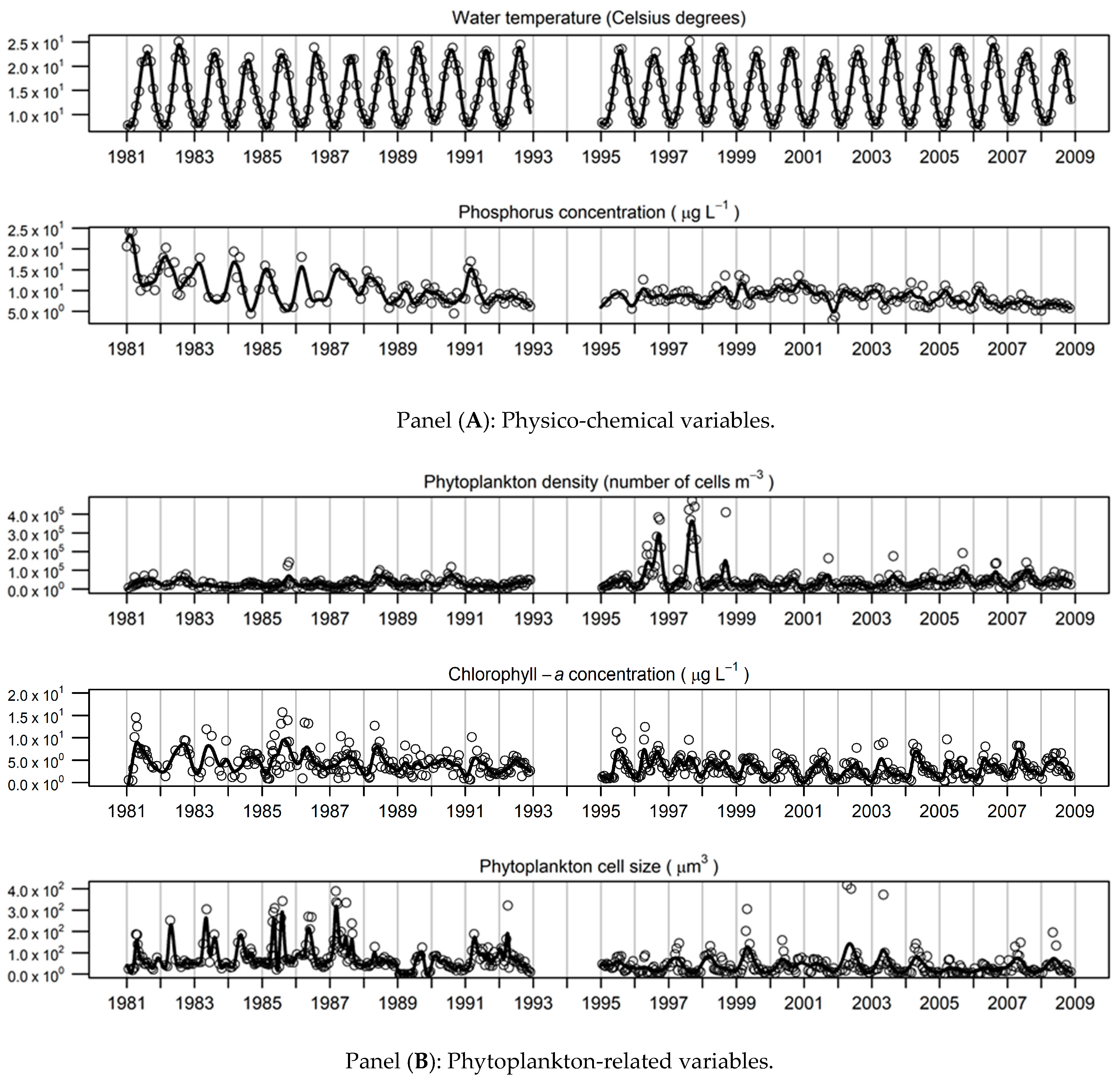
3.1. Long-Term Limnological Change

Thermal conditions changes in Lake Maggiore over the study period. Mean summer temperature across the 0–20 m depth averaged 21.2 °C between 1981 and 1992 and 21.9 °C between 1995 and 2008, as also observed in previous studies [42]. Lake Maggiore underwent a gradual warming of the epilimnion in the decade 1988–1998, according to the trend of increasing heat content of the deep Italian lakes, pointed out by Carrara et al. [43]. The period was characterized by strong fluctuations, in particular between 1988 and 1992. Since 1999, the increase of water temperature was less evident, probably because of the occurrence of particular hydro-meteorological mechanisms reducing the heat content of the water column [43,44]. Lake Maggiore also experienced a dramatic reduction in total phosphorus (TP) concentration over the study period. Mean TP_mix concentration declined from 10.9 μg L⁻¹ between 1981 and 1992, to 8.4 μg L⁻¹ between 1995 and 2008. An exceptionally high value, of 17 μg L⁻¹, was detected in 1991, after the lake’s complete winter overturn. Over a general increase, a second peak value was recorded in 1999, after another complete overturn. The overall increase to stable values of 11 μg L⁻¹ after 2000 could be mainly explained by meteorological-climatic conditions, rather than by an eutrophication reversal [45]. Eutrophication abatement results were mixed, however, as mean chlorophyll-a concentration fell sharply (from 4.7 to 3.4 µg L⁻¹) between these periods, though results for phytoplankton biomass were less clear (1830 vs. 1181 mm³ m⁻³, respectively).

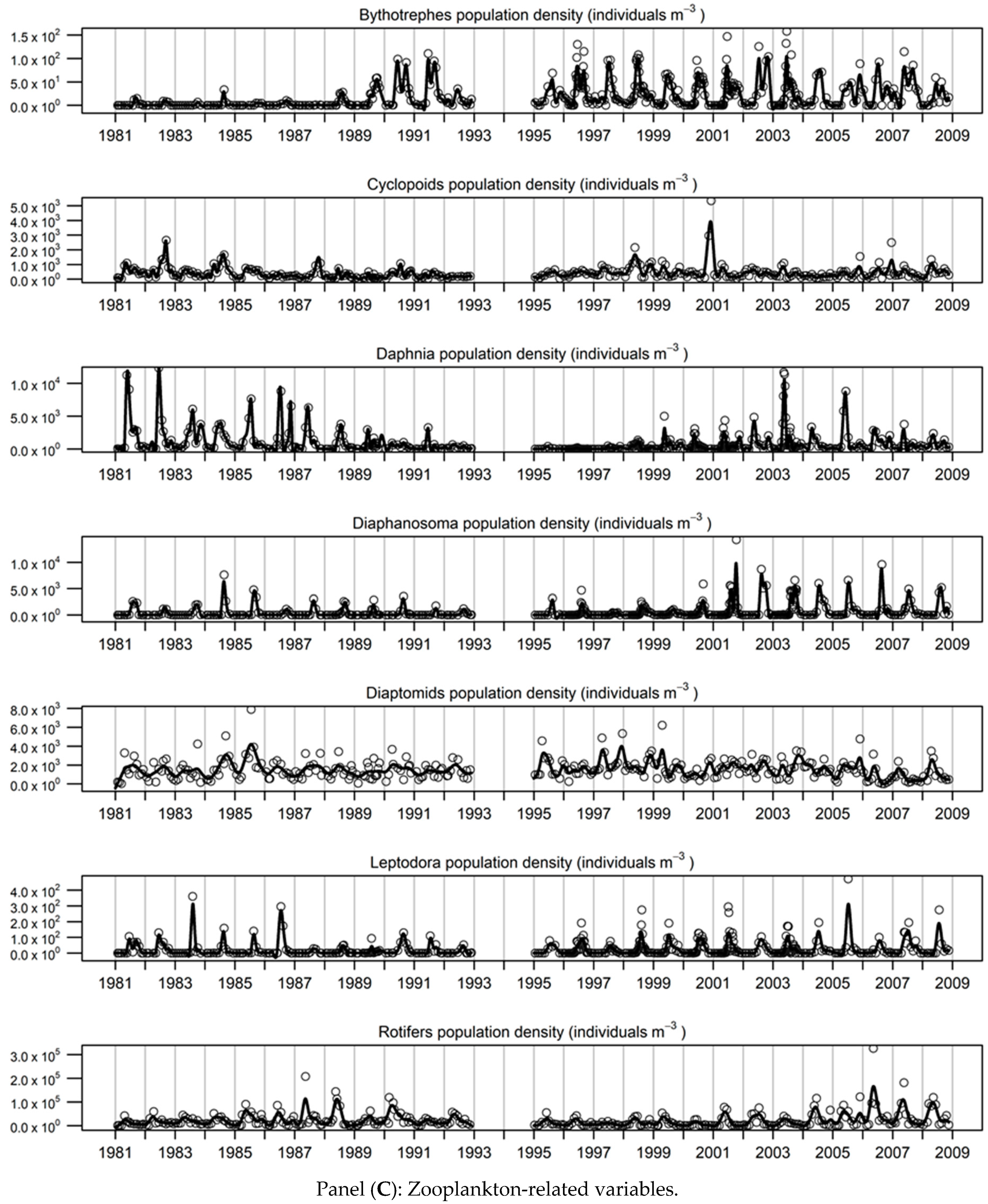
3.2. Description of the Smoothed Time-Series

The observed and smoothed time-series of the considered variables are represented in Figure 1. A visual inspection of the graphs in Figure 1 suggests that the smoothed curves have a good fit to the overall trend of the corresponding variables. Major variations in phosphorus concentration, phytoplankton cell size and chlorophyll-a concentration during 1981–1988 matched an increase in variability and mean density of Bythotrephes longimanus, and a decrease in between-year variability and mean annual population densities of Bosmina (mainly, Eubosmina longispina) and Daphnia (D. longispina-galeata gr.). The increased within-year variability in Bythotrephes observed during the 1990s was maintained across the second time period, whereas Daphnia and Bosmina variability and population density increased between 2002–2008, along with Diaphanosoma brachyurum. During 2002–2008, variability of diaptomid copepods seems to have decreased slightly relative to the periods 1981–1992 and 1995–2000. Rotifer (and to lesser extent) Leptodora kindtii density were characterized by increased variability during the last five years of the 1995-2008 period. In addition, rotifer communities changed dramatically through time, with the mean ratio of raptorial to microphagous species abundance decreasing from 1.5 ± 2.0 (mean ± st.dev.) during 1981–1992 to 0.5 ± 0.6 (mean ± st.dev.) during 1995–2002 [42,46].

Phytoplankton density was highly variable during the 1996–1998 interval. Phosphorus concentration, phytoplankton cell size, chlorophyll-a concentration, Bosmina and Daphnia population density all exhibited a more variable trend during 1981–1992 than during 1995–2008 using both observed and smoothed time-series data (Figure 1). Conversely, phytoplankton density, Bythothrephes, cyclopoid copepods, and Diaphanosoma population density were more variable between 1995–2008.

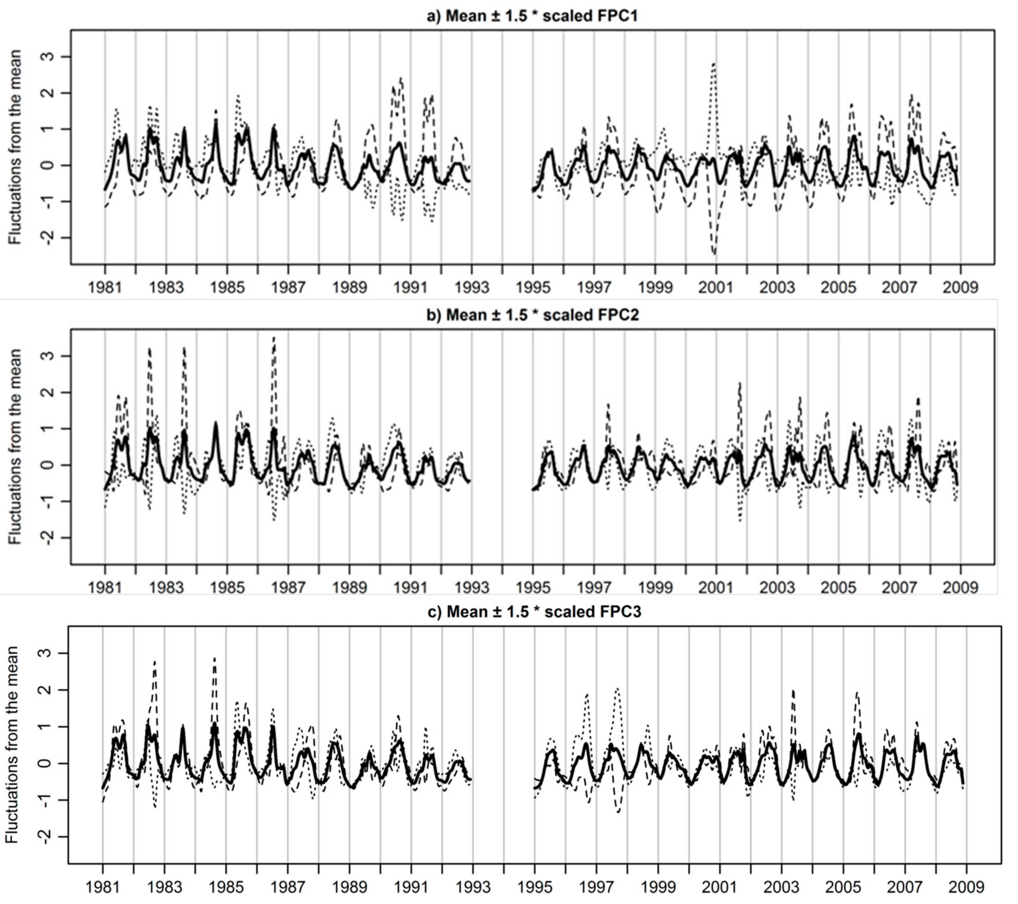
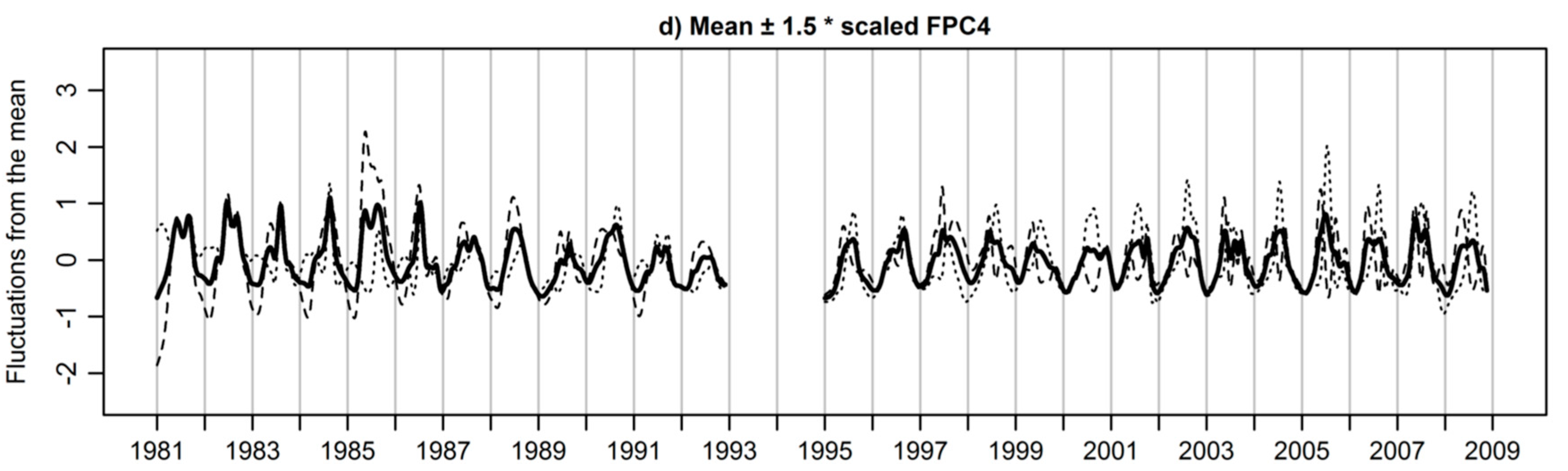
3.3. Extracted Functional Principal Components

For both periods, the first four rotated FPCs were retained, and explained 55% and 65% of the overall variation of smoothed standardized variables for 1981–1992 and 1995–2008 periods, respectively. The effect of each FPC (denoted FPC1-4 in decreasing order of explained variation for both periods) on the trend of considered variables is represented in Figure 2. This shows, for the two periods, the overall mean (continuous line) of the smoothed standardized variables, along with curves representing the effect of adding (dashed line) or subtracting (dotted line) each scaled FPC on the mean. The FPC1 corresponds to an overall increasing trend in both the 1981–1992 and 1995–2008 periods, as in each case the dotted (increasing) and dashed (decreasing) lines cross the graph of the overall mean as time increases (Figure 2a). In addition, the FPC1 for the 1981–1992 period also corresponds to more extreme of mid-year values during the 1990s. Similarly, the FPC1 for 1995–2008 corresponds to more extreme mid-year values during the second half of the 2000s, as well as very extreme values at the end of 2000. Fluctuations around the overall mean for FPC1 mirror the high variability of phosphorus concentration and of Bythotrephes density during 1981–1993.

Dynamics of the other principal components (FPC2-4) are highlighted in Figure 2b,c. Briefly, FPC2 corresponds to more extreme values during the 1980s (especially in 1981, 1982, 1983 and 1986) and during the 2000s. Strong deviations observed during the 1980s can be attributed to fluctuations of two parameters with the highest scores on this component: The density of Bosmina and the concentration of chlorophyll-a. FPC3 gives more weight to 1982 and 1984, as well as 1996, 1997, 2003, and 2005. The high variability, in some of these years, of chlorophyll concentration and Daphnia density explains much of the observed fluctuations around the overall mean. Lastly, FPC4 gives more weight to 1985 and the 2000s, especially 2005. The observed perturbations from the mean during the 2000s can be explained by variation in Leptodora population density.

3.4. Functional Principal Components Scores

The scores for the FPC1 show how, during 1981–1992, Bythotrephes population density (score 48.2) increased dramatically during the 1990s, while phosphorus concentration decreased over time (score −37.8) (

Table 1. Functional Principal Components (FPCs) scores for three different groups (in italics) of considered variables. The most extreme positive and negative scores are highlighted (italics) for each FPC. Pop. dens. = population density.

	Functional Principal Components (FPCs) Scores
Calendar period	1981–1992				1995–2008
Variables	FPC1	FPC2	FPC3	FPC4	FPC1	FPC2	FPC3	FPC4
Physico-Chemical
Water temperature	30.5	11.9	16.7	13.1	30.2	10.9	−12.6	−25.7
Phosphorus concentration	−37.8	−16.6	−25.9	−46.9	−45.2	−15.2	−14.2	−2.0
Phytoplankton-related
Phytoplankton pop. dens.	13.7	−10.6	12.6	−3.8	8.6	1.1	−39.6	5.5
Chlorophyll-a concentration	−11.2	−9.7	3.8	8.6	12.6	−29.1	−16.5	1.9
Phytoplankton cell size	−20.8	−18.7	−21.0	3.9	−17.0	−19.5	12.1	10.4
Zooplankton-related
Bosmina pop. dens.	−13.0	37.5	−17.7	26.0	20.6	46.1	1.4	20.0
Bythotrephes pop. dens.	48.2	−17.2	−14.7	−17.1	19.8	1.0	−1.8	−16.6
Cyclopoid pop. dens.	−16.0	−10.6	41.8	0.1	−38.5	1.4	7.6	15.9
Daphnia pop. dens.	−14.0	34.6	−4.6	7.9	9.2	−15.0	33.8	17.9
Diaphanosoma pop. dens.	12.4	−2.1	24.8	−9.7	4.3	34.0	10.2	−32.9
Diaptomid pop. dens.	−1.3	−9.1	2.9	13.8	−28.1	5.4	−3.0	24.7
Leptodora pop. dens.	13.3	31.8	4.6	−12.2	11.4	0.7	4.7	−33.5
Rotifer pop. dens.	−4.1	−21.1	−23.2	16.3	12.0	−21.8	18.0	14.4

). Phosphorus concentration maintained a similar trend during 1995–2008 (score −45.2), while water temperature increased during both considered periods (score of 30.5 in 1981–1992 and of 30.2 in 1995–2008), fitting FPC1 better than Bythotrephes density (score 19.8) (Table 1).

Scores for FPC2 during 1981–1992 show how this principal component had the most effect on Bosmina density (score 37.5), which reached higher values at the start of 1980 (Figure 1c). By contrast, rotifer density (score −21.1) was stable at the start of the 1980s and more variable at the end of the decade (Table 1). During 1995-2008, FPC2 was affected in a similar way by both Bosmina density (score 46.1) and rotifer density (score −21.8). Chlorophyll-a concentration (score −29.1), which reaches its lowest values in 2001 (Figure 1b), also becomes important for FPC2 in this period.

The scores for FPC3 during 1981–1992 show that this FPC were most affected by cyclopoid copepod density (score 41.8), which reached high values in both 1982 and 1984 (Figure 1c), and phosphorus (score −25.9) which reached a minimum concentration in 1984 as oligotrophication proceeded (Figure 1a). Between 1995–2008, FPC3 was most affected by Daphnia density (score 33.8), which reached high values in 2003 and 2005 (Figure 1b), and phytoplankton density (score −39.6), which had very high values in 1996–1997 (Figure 1b).

Lastly, in 1981–1992, FPC4 was most affected by phosphorus concentration (score −46.9), which had a minimum in 1985 (Figure 1a), and Bosmina density (score 26.0), which reached one of its highest values in the same year (Figure 1c). During 1995–2008, FPC4 was most affected by diaptomid copepod density (score 24.7), whose within-year dynamic changed substantially during the 2000s (Figure 1c), and Leptodora density (score −33.5), which reached high values in the summer 2005 (Figure 1c).

4. Discussion

We used Functional Data Analysis to describe long-term abiotic and biotic dynamics of Lake Maggiore. FDA has features that made it ideal for long-term studies like ours. FDA provides a useful framework to analyzing short and long-term dynamics of a lake ecosystem, its data smoothing respects the continuous nature of the underlying biological and physico-chemical processes while accounting for potential irregularities during measurement periods, and it allows analysis of dominant modes of variation in trajectories of measured parameters in a way that respects the time ordering of observations.

FPCA proved useful in identifying Lake Maggiore’s responses to both trophic and climatic variability. Among the extracted FPCs, FPC1 illustrated the increasing trend of Bythotrephes population density and decreasing trend of phosphorus concentration at the beginning of oligotrophication, between 1981–1992. In 1996 and 1997, large blooms of ultraplankton—including small cyanobacteria—occurred in the lake, coincident with very low mean densities of Daphnia. However, as lake productivity declined owing to phosphorus abatement [25,26,27,42] below 15 mg m⁻³, the level at which TP mix becomes limiting for phytoplankton growth [27], Bythotrephes increased in density, while Daphnia declined [47,48]. A previous study has demonstrated that Bythotrephes occurs primarily in European lakes with low summer chlorophyll concentration [49], consistent with its resurgence during oligotrophication in Lake Maggiore. The decline in Daphnia (see Table 1) could be due to either reduced food supply (bottom-up response) or to increased predation by Bythotrephes (top-down response), or both. Available evidence suggests that food reduction may have caused the decline between 1983 and 1987, as declining phytoplankton stocks may have caused food limitation. However, beyond this point, predation by Bythotrephes likely accelerated the decline in Daphnia density, as the latter’s death rate increased when Bythotrephes populations surged beyond 20 ind·m⁻³ beginning in 1987 [47]. Larger and seemingly more potent Bythotrephes sharply curtail crustacean abundance when present at levels beyond ~2 ind·m⁻³ in Ontario lakes [50]. Interestingly, Leptodora and Bythotrephes have inverse distributions in Ontario lakes with the former often replaced by the latter after it invades new systems [51]. These species show no such pattern in Lake Maggiore, where both species are native and presumably co-adapted to one another’s presence. In addition, body size differences between the species are much smaller than in Ontario lakes, suggesting less physical dominance by Bythotrephes.

In addition to dramatic changes in population density, Bythotrephes has also experienced large shifts in seasonality, with peak density shifting from August to May (see Figure 1c) as the lake warmed [31,36]. This, in turn, may have increased predation pressure on Daphnia [47,48], which previously typically achieved population maxima in July but now peaks months earlier [52]. The second phase of Daphnia increase, during full and stable oligotrophy, resulted both from Daphnia’s ability to cope with increased invertebrate predation by means of changes in population phenology and by a release from fish predation consequent to a decrease in coregonid (i.e., whitefish) abundance, which also favors consumption of Bythotrephes over Daphnia [53,54]. Previous research has demonstrated strong preference of coregonid fishes for Bythotrephes prey [55].

Oligotrophication was associated with a decline in phytoplankton density between 1995–2008, as clearly shown by both FPC2 and FPC3. However, this reduction in plankton food resources does not seem to have affected most cladocerans as FPC2 highlighted an increase of Bosmina whereas FPC3 captured the same trend for Daphnia. We hypothesize that the long-term increase in water temperature stimulated the growth of Daphnia—as demonstrated by peak population density achieved during the heat wave of summer 2003—possibly owing to reduced development time [56,57].

FPC analyses are compatible with a response by planktonic communities to both temperature increase and total phosphorus concentration decline. The former variable enhances primary production with its consequent indirect, positive effect on herbivores and negative effect on Bythotrephes, whereas the latter appeared to favor Bythotrephes and its strong top-down effects.

Raptorial dominance declined after 1988 concomitant with changes in cladocerans: Bythotrephes longimanus increased by an order of magnitude, Daphnia gr. hyalina-galeata showed a sharp decline and small cladocerans such as Eubosmina longispina and Diaphanosoma brachyurum increased [26,29]. An increase in B. longimanus releases rotifers, especially large Conochilus hippocrepis (or C. volvox ehrbg, Schrank, 1803) colonies, from competition with cladocerans [58]. The decrease in abundance and mean size of phytoplankton cells with lake restoration might have enhanced microphagous species able to ingest multiple food items of ~15–20 μm, while raptorials prefer larger particles [46,59,60,61]. Decreased abundance of competitors and decreased food size, therefore, might enhance microphagous species, while raptorial species were able to coexist with their competitors [46,59,62]. Large (≥1 mm diameter) Conochilus colonies have feeding rates comparable to Daphnia and lead to a seasonal increase in water clarity like that caused by Daphnia grazing [58].

The response of rotifers to changes in the macrozooplankton assemblage is probably more complex than previously hypothesized. Manca [63] reported a strong increase of Conochilus hippocrepis in Lake Maggiore when Bythotrephes became increasingly abundant in the late 1980s. However, the FPCA highlighted that the increase in rotifer density preceded that of Bythotrephes and the two populations seemed to follow divergent development trajectories during the periods examined. Therefore, the behavior of rotifers during oligotrophication of Lake Maggiore is different from that observed in Ontario lakes, where they benefited numerically from competitive release associated with reduced density of Daphnia competitors when Bythotrephes was abundant [64]. Once established, C. hippocrepis populations would be relatively immune to growing Bythotrephes populations owing to its gelatinous colonial matrix.

Exceptional meteoclimatic events can be detected over the long term [65]. As an example, the almost complete vertical mixing of February 1999 and the record flood of 2000 were also reported to impact zooplankton seasonal dynamics. As reported by Manca, Cavicchioni and Morabito [66], nutrient replenishment of surface waters from deeper waters consequent to vertical mixing triggered a cascading effect, involving all planktonic communities. Larger input of new nutrients stimulated phytoplankton productivity and higher food availability for herbivorous zooplankton, resulting in an increased density of rotifers, copepods, and cladocerans, as well as of Daphnia clutch size. Finally, an increase of predatory cladocerans (Leptodora) was recorded in July, five months after the complete mixing episode. Temperature can control nutrient supply, by affecting the extent of the mixing layer at the time of spring overturn: This mechanism is particularly effective in deep Italian lakes [67,68], where a strong link between winter temperature, mixing depth and was established. Similarly, the record flood of 2000 is well identified in the time series analyzed. Impact on zooplankton included detection in the pelagic of littoral taxa such as Bosmina longirostris and altered the seasonality of Bythotrephes longimanus [52].

5. Conclusions

Long-term data allow for disentangling the contribution of different stressors to changes in response variables. In Lake Maggiore, many stressors altered the system during the 20th century, prominent among them cultural eutrophication in the 1960s and 1970s. Phosphorus abatement began in 1977, with strong observed TP reductions observed thereafter. This change had pronounced effects on numerous biological response variables, notably chlorophyll-a concentration and phytoplankton community size composition, and Daphnia population density. We also observed increased variability and enhanced population density of the invertebrate predator Bythotrephes longimanus during the initial study period, and by small-bodied cladocerans Bosmina and Diaphanosoma during the second period. The increase in population density and inter-annual variability of small cladocerans might be viewed as a response to decreasing Daphnia population density. Bythotrephes population densities increased during the second study period, resulting in enhanced predation pressure on Daphnia prey. Impact on Daphnia during this period was reduced by a temperature increase - which served to reduce its development time and increase its birth rate - and by earlier phenology such that it exhibited less temporal overlap with Bythotrephes. As previously observed, over the long term, both cladocera and rotifers responded more clearly to eutrophication reversal and to warming, than copepods. The latter seem to be more influenced by exceptional meteoclimatic events, such as mixing depth. This result agrees well with analyses of ecological roles of Lake Maggiore freshwater zooplankton by carbon and nitrogen stable isotope analyses. Copepods, particularly cyclopoids, occupy a distinct functional group from the other zooplankton secondary consumers, which is an observation also made in previous studies [54,69,70].

References

1. Binelli, A.; Provini, A. DDT is still a problem in developed countries: The heavy pollution of Lake Maggiore. Chemosphere 2003, 52, 717–723. [Google Scholar] [CrossRef]
2. Vinebrooke, R.D.; Cottingham, K.L.; Norberg, J.; Scheffer, M.; Dodson, S.I.; Maberly, S.C.; Sommer, U. Impacts of multiple stressors on biodiversity and ecosystem functioning: The role of species co-tolerance. Oikos 2004, 104, 451–457. [Google Scholar] [CrossRef]
3. Yan, N.D.; Girard, R.; Heneberry, J.H.; Keller, W.B.; Gunn, J.M.; Dillon, P.J. Recovery of copepod, but not cladoceran, zooplankton from severe and chronic effects of multiple stressors. Ecol. Lett. 2004, 7, 452–460. [Google Scholar] [CrossRef]
4. Schindler, D.W. Recent advances in the understanding and management of eutrophication. Limnol. Oceanogr. 2006, 51, 356–363. [Google Scholar] [CrossRef] [Green Version]
5. Jeziorski, A.; Yan, N.D.; Paterson, A.M.; DeSellas, A.M.; Turner, M.A.; Jeffries, D.S.; Keller, B.; Weeber, R.C.; McNicol, D.K.; Palmer, M.E.; et al. The widespread threat of calcium decline in fresh waters. Science 2008, 322, 1374–1377. [Google Scholar] [CrossRef] [PubMed]
6. Ormerod, S.J.; Dobson, M.; Hildrew, A.G.; Townsend, C.R. Multiple stressors in freshwater ecosystems. Freshw. Biol. 2010, 55 (Suppl. 1), 1–4. [Google Scholar] [CrossRef] [Green Version]
7. Strayer, D.L. Alien species in fresh waters: Ecological effects, interactions with other stressors, and prospects for the future. Freshw. Biol. 2010, 55 (Suppl. 1), 152–174. [Google Scholar] [CrossRef]
8. Maberly, S.C.; Elliott, J.A. Insights from long-term studies in the Windermere catchment: External stressors, internal interactions and the structure and function of lake ecosystems. Freshw. Biol. 2012, 57, 233–243. [Google Scholar] [CrossRef]
9. Guilizzoni, P.; Levine, S.N.; Manca, M.; Marchetto, A.; Lami, A.; Ambrosetti, W.; Brauer, A.; Gerli, S.; Carrara, E.A.; Rolla, A.; et al. Ecological effects of multiple stressors on a deep lake (Lago Maggiore, Italy) integrating neo and paleolimnological approaches. J. Limnol. 2012, 71, 1–22. [Google Scholar] [CrossRef]
10. Allan, A.J.D.; McIntyre, P.B.; Smitha, S.D.P.; Halpern, B.S.; Boyer, G.L.; Buchsbaum, A.; Burton, G.A., Jr.; Campbell, L.M.; Chadderton, W.L.; Ciborowski, J.J.H.; et al. Joint analysis of stressors and ecosystem services to enhance restoration effectiveness. Proc. Nat. Acad. Sci. USA 2013, 110, 372–377. [Google Scholar] [CrossRef]
11. Verdonschot, P.F.M.; Spears, B.M.; Feld, C.K.; Brucet, S.; Keizer-Vlek, H.; Borja, A.; Elliott, M.; Kernan, M.; Johnson, R.F. A comparative review of recovery processes in rivers, lakes, estuarine and coastal waters. Hydrobiologia 2013, 704, 453–474. [Google Scholar] [CrossRef]
12. Smol, J.P.; Wolfe, A.P.; Birks, H.J.B.; Douglas, M.S.V.; Jones, V.J.; Korhola, A.; Pienitz, R.; Rühland, K.; Sorvari, S.; Antoniades, D.; et al. Climate-driven regime shifts in the biological communities of arctic lakes. Proc. Nat. Acad. Sci. USA 2005, 102, 4397–4402. [Google Scholar] [CrossRef] [Green Version]
13. Moss, B. Climate change, nutrient pollution and the bargain of Dr Faustus. Freshw. Biol. 2010, 55 (Suppl. 1), 175–187. [Google Scholar] [CrossRef] [Green Version]
14. Thompson, P.L.; Shurin, J.B. Regional zooplankton biodiversity provides limited buffering of pond ecosystems against climate change. J. Anim. Ecol. 2012, 81, 251–259. [Google Scholar] [CrossRef] [PubMed]
15. Jackson, M.C.; Loewen, C.J.G.; Vinebrooke, R.D.; Chimimba, C.T. Net effects of multiple stressors in freshwater ecosystems: A meta-analysis. Glob. Chang. Biol. 2016, 22, 180–189. [Google Scholar] [CrossRef] [PubMed]
16. Hering, D.; Borja, A.; Carvalho, L.; Feld, C.K. Assessment and recovery of European water bodies: Key messages from the WISER project. Hydrobiologia 2013, 704, 1–9. [Google Scholar] [CrossRef]
17. Jeppesen, E.; Sondergaard, M.; Jensen, J.P.; Havens, K.E.; Anneville, O.; Carvalho, L.; Coveney, M.F.; Deneke, R.; Dokulil, M.; Foy, B.; et al. Lake responses to reduced nutrient loading—An analysis of contemporary long-term data from 35 case studies. Freshw. Biol. 2005, 50, 1747–1771. [Google Scholar] [CrossRef]
18. Schindler, D.W. The dilemma of controlling eutrophication of lakes. Proc. R. Soc. B 2012, 279, 4322–4333. [Google Scholar] [CrossRef]
19. Yan, N.D.; Pawson, T.W. Changes in the crustacean zooplankton community of Harp Lake, Canada, following invasion by Bythotrephes cederstrœmi. Freshw. Biol. 1997, 37, 409–425. [Google Scholar] [CrossRef]
20. Straile, D.; Geller, W. The response of Daphnia to changes in trophic status and weather patterns: A case study from Lake Constance. ICES J. Mar. Sci. 1998, 55, 775–782. [Google Scholar] [CrossRef]
21. May, L.; Spears, B.M. A history of scientific research at Loch Leven, Kinross, Scotland. Hydrobiologia 2012, 681, 3–9. [Google Scholar] [CrossRef]
22. Lottig, N.R.; Carpenter, S.R. Interpolating and forecasting lake characteristics using long-term monitoring data. Limnol. Oceanogr. 2012, 57, 1113–1125. [Google Scholar] [CrossRef]
23. Ramsay, J.; Silverman, B.W. Functional Data Analysis, 2nd ed.; Springer: New York, NY, USA, 2005. [Google Scholar]
24. de Bernardi, R.; Giussani, G.; Manca, M.; Ruggiu, D. Long-term dynamics of plankton communities in Lago Maggiore (N. Italy). Internationale Vereinigung für Theoretische und Angewandte Limnologie: Verhandlungen 1988, 23, 729–733. [Google Scholar] [CrossRef]
25. de Bernardi, R.; Giussani, G.; Manca, M.; Ruggiu, D. Trophic status and the pelagic system in Lake Maggiore. Hydrobiologia 1990, 191, 1–8. [Google Scholar] [CrossRef]
26. Manca, M.; Ruggiu, D. Consequences of pelagic food-web changes during a long-term lake oligotrophication process. Limnol. Oceanogr. 1998, 43, 1368–1373. [Google Scholar] [CrossRef] [Green Version]
27. Sas, H. Lake Restoration by Reduction of Nutrient Loading: Expectations, Experiences, Extrapolation; Academic Verlag: St. Augustin, FL, USA, 1989. [Google Scholar]
28. de Bernardi, R.; Canale, C. Ricerche pluriennali (1948–1992) sull’ecologia dello zooplancton del Lago Maggiore. Doc Ist. Ital. Hydrobiol. 1995, 55, 1–68. [Google Scholar]
29. Manca, M.; Calderoni, A.; Mosello, R. Limnological research in Lago Maggiore: Studies on hydrochemistry and plankton. Memorie Istituto Italiano di Idrobiologia 1992, 50, 171–200. [Google Scholar]
30. Tonolli, L. Holomixy and oligomixy in Lake Maggiore: Inference on the vertical distribution of zooplankton. Verh. Int. Ver. Limnol. 1969, 17, 231–236. [Google Scholar] [CrossRef]
31. Manca, M.; DeMott, W.R. Response of the invertebrate predator Bythotrephes to a climate-linked increase in the duration of a refuge from fish predation. Limnol. Oceanogr. 2009, 54 Pt 2, 2506–2512. [Google Scholar] [CrossRef]
32. Arca, G.; Barbanti, L. Annuario dell’Osservatorio Meteorologico di Pallanza; Documenta Ist. Ital. Idrobiol; Consiglio Nazionale delle Ricerche, Istituto Italiano di Idrobiologia: Pallanza, Italy, 1991; pp. 1–83. (In Italian) [Google Scholar]
33. Barbanti, L. Annuario dell’Osservatorio Meteorologico di Pallanza; Documenta Ist. Ital. Idrobiol; Consiglio Nazionale delle Ricerche, Istituto Italiano di Idrobiologia: Pallanza, Italy, 1997; pp. 1–81. (In Italian) [Google Scholar]
34. Ambrosetti, W.; Barbanti, L.; Rolla, A. Annuario dell’Osservatorio Meteorologico di Pallanza. 1997–2003; CNR Istituto per lo Studio degli Ecosistemi: Verbania Pallanza, Italy, 2006; pp. 1–38. [Google Scholar]
35. Ambrosetti, W.; Barbanti, L.; Rolla, A. Annuario dell’Osservatorio Meteorologico di Pallanza. 2004–2005; CNR Istituto per lo Studio degli Ecosistemi: Verbania Pallanza, Italy, 2006; pp. 1–70. [Google Scholar]
36. Ambrosetti, W.; Barbanti, L.; Rolla, A. Annuario dell’Osservatorio Meteorologico di Pallanza. 2006; CNR Istituto per lo Studio degli Ecosistemi: Verbania Pallanza, Italy, 2007; pp. 1–51. [Google Scholar]
37. Ambrosetti, W.; Barbanti, L.; Rolla, A. Annuario dell’Osservatorio Meteorologico di Pallanza. 2007; CNR Istituto per lo Studio degli Ecosistemi: Verbania Pallanza, Italy, 2008; pp. 1–56. [Google Scholar]
38. Lorenzen, C.J. Determination of chlorophyll and pheo-pigments: Spectrophotometric equations. Limnol. Oceanogr. 1967, 12, 343–346. [Google Scholar] [CrossRef]
39. Rott, E. Some results from phytoplankton counting intercalibrations. Schweiz. Z. Hydrol. 1981, 43, 34–63. [Google Scholar] [CrossRef]
40. Lund, J.W.G.; Kipling, C.; Le Cren, E.D. The inverted microscope method of estimating algal numbers and the statistical basis of estimations by counting. Hydrobiologia 1958, 11, 143–170. [Google Scholar] [CrossRef]
41. Wacklin, P.; Hoffmann, L.; Komárek, J. Nomenclatural validation of the genetically revised cyanobacterial genus. Fottea 2009, 9, 59–64. [Google Scholar] [CrossRef]
42. Morabito, G.; Manca, M. Eutrophication and recovery of the large and deep subalpine Lake Maggiore: Patterns, trends and interactions of planktonic organisms between trophic and climatic forcings. In Chapter 6 in Eutrophication; Lambert, A., Roux, C., Eds.; Nova Science Publishers: New York, NY, USA, 2013; ISBN 978-1-62808-498-6. [Google Scholar]
43. Carrara, E.; Ambrosetti, W.; Barbanti, L. The management of Lake Maggiore water levels: A study of low water episodes. In Proceedings of the Symposium on the Role of Hydrology in Water Resources Management, Capri, Italy, 29–31 October 2008; Volume 327, pp. 114–123. [Google Scholar]
44. Ambrosetti, W.; Barbanti, L.; Carrara, E. Mechanisms of hypolimnion erosion in a deep lake (Lago Maggiore, N. Italy). J. Limnol. 2010, 69, 3–14. [Google Scholar] [CrossRef]
45. Ruggiu, D.; Morabito, G.; Panzani, P.; Pugnetti, A. Trends and relations among basic phytoplankton characteristics in the course of the long-term oligotrophication of Lago Maggiore (Italy). Hydrobiologia 1998, 369–370, 243–257. [Google Scholar] [CrossRef]
46. Obertegger, U.; Manca, M. Response of rotifer functional groups to changing trophic state and crustacean community. J. Limnol. 2011, 70, 231–238. [Google Scholar] [CrossRef]
47. Manca, M.; Ramoni, C.; Comoli, P. The decline of Daphnia hyalina galeata in Lago Maggiore: A comparison of the population dynamics before and after oligotrophication. Aquat. Sci. 2000, 62, 142–153. [Google Scholar] [CrossRef]
48. Manca, M.; Portogallo, M.; Brown, M. Shifts in phenology of Bythotrephes longimanus and its modern success in Lake Maggiore as a result of changes in climate and trophy. J. Plankton Res. 2007, 29, 515–525. [Google Scholar] [CrossRef]
49. MacIsaac, H.J.; Ketelaars, H.A.M.; Girgorovich, I.A.; Ramcharan, C.W.; Yan, N.D. Modeling Bythotrephes longimanus invasions in the Great Lakes basin based on its European distribution. Arch. Hydrobiol. 2000, 141, 1–21. [Google Scholar] [CrossRef]
50. Boudreau, S.A.; Yan, N.D. The differing crustacean zooplankton communities of Canadian Shield lakes with and without the nonindigenous zooplanktivore Bythotrephes longimanus. Can. J. Fish. Aquat. Sci. 2003, 60, 1307–1313. [Google Scholar] [CrossRef]
51. Weisz, E.J.; Yan, N.D. Shifting invertebrate zooplanktivores: Watershed-level replacement of the native Leptodora by the non-indigenous Bythotrephes in Canadian Shield lakes. Biol. Invasions 2011, 13, 115–123. [Google Scholar] [CrossRef]
52. Manca, M. Considerazioni generali sull’evoluzione a lungo termine dei popolamenti planctonici. In Ecologia delle Acque Interne. Ricerche sull’evoluzione del Lago Maggiore. Aspetti limnologici. Programma quinquennale; Campagna 2002; Commissione Internazionale per la protezione delle acque italo-svizzere, sezione di Idrobiologia, C.N.R.-I.S.E.: Verbania, Italy, 2014; pp. 134–136. (In Italian) [Google Scholar]
53. de Bernardi, R.; Giussani, G.; Manca, M. Cladocera: Predators and Prey; Springer: Dordrecht, The Netherlands, 1987; pp. 225–243. [Google Scholar]
54. Visconti, A.; Volta, P.; Fadda, A.; Di Guardo, A.; Manca, M. Seasonality, littoral versus pelagic carbon sources, and stepwise δ15N-enrichment of pelagic food web in a deep subalpine lake: The role of planktivorous fish. Can. J. Fish. Aquat. Sci. 2013, 71, 436–446. [Google Scholar] [CrossRef]
55. Coulas, R.A.; MacIsaac, H.J.; Dunlop, W. Selective predation by lake herring (Coregonus artedi) on exotic zooplankton (Bythotrephes cederstroemi) in Harp Lake, Ontario. Freshw. Biol. 1998, 40, 343–356. [Google Scholar] [CrossRef]
56. Visconti, A.; Manca, M.; De Bernardi, R. Eutrophication-like response to climate warming: an analysis of Lago Maggiore (N. Italy) zooplankton in contrasting years. J. Limnol. 2008, 67, 87–92. [Google Scholar] [CrossRef]
57. Gillooly, J.F.; Charnov, E.L.; West, G.B.; Savage, V.M.; Brown, J. Effects of size and temperature on developmental time. Nature 2003, 417, 70–73. [Google Scholar] [CrossRef]
58. Manca, M.; Sonvico, D. Seasonal variations in population density and size structure of Conochilus in Lago Maggiore: A biannual study. Mem. Ist. Ital. Idrobiol. 1996, 54, 97–108. [Google Scholar]
59. Obertegger, U.; Smith, H.A.; Flaim, G.; Wallace, R.L. Using the guild ratio to characterize pelagic rotifer communities. Hydrobiologia 2011, 662, 157–162. [Google Scholar] [CrossRef]
60. Pourriot, R. Food and feeding habits of Rotifera. Arch. Hydrobiol. Beih. Ergebn. Limnol. 1977, 8, 243–260. [Google Scholar]
61. Wallace, R.L.; Snell, T.W.; Ricci C Nogrady, T. Rotifera Volume 1: Biology, Ecology and Systematics. In Guides to the Identification of the Microinvertebrates of the Continental Waters of the World, 2nd ed.; Dumont, H.J.F., Ed.; Kenobi Productions: Ghent, Belgium; Backhuys Publishers: Leiden, The Netherlands, 2006; Volume 23. [Google Scholar]
62. temberger, R.S.; Gilbert, J.J. Rotifer threshold food concentrations and the size-efficiency hypothesis. Ecology 1987, 68, 181–187. [Google Scholar] [CrossRef]
63. Manca, M. Invasions and re-emergences: An analysis of the success of Bythotrephes in Lago Maggiore (Italy). J. Limnol. 2011, 70, 76–82. [Google Scholar] [CrossRef]
64. Hovius, J.T.; Beisner, B.E.; McCann, K.S.; Yan, N.D. Indirect food web effects of Bythotrephes invasion: Responses by the rotifer Conochilus in Harp Lake, Canada. Biol. Invasions 2007, 9, 233–243. [Google Scholar] [CrossRef]
65. Manca, M.; Torretta, B.; Comoli, P.; Amsinck, S.L.; Jeppesen, E. Major changes in trophic dynamics in large, deep sub-alpine Lake Maggiore from 1940s to 2002: A high resolution comparative paleo-neolimnological study. Freshw. Biol. 2007, 52, 2256–2269. [Google Scholar] [CrossRef]
66. Manca, M.; Cavicchioni, N.; Morabito, G. First observations on the effect of a complete, exceptional overturn of Lake Maggiore on plankton and primary productivity. Int. Rev. Hydrobiol. 2000, 85, 209–222. [Google Scholar] [CrossRef]
67. Salmaso, N.; Buzzi, F.; Garibaldi, L.; Morabito, G.; Simona, M. Effects of nutrient availability and temperature on phytoplankton development: A case study from large lakes south of the Alps. Aquat. Sci. 2012, 74, 555–570. [Google Scholar] [CrossRef]
68. Manca, M.; Rogora, M.; Salmaso, N. Inter-annual climate variability and zooplankton: Applying teleconnection indices to two deep subalpine lakes in Italy. J. Limnol. 2014, 74. [Google Scholar] [CrossRef]
69. Visconti, A.; Caroni, R.; Rawcliffe, R.; Fadda, A.; Piscia, R.; Manca, M. Defining Seasonal Functional Traits of a Freshwater Zooplankton Community Using δ13C and δ15N Stable Isotope Analysis. Water 2018, 10, 108. [Google Scholar] [CrossRef]
70. Visconti, A.; Manca, M. Seasonal changes in the δ13C and δ15N signatures of the Lago Maggiore pelagic food web. J. Limnol. 2011, 70, 263–271. [Google Scholar] [CrossRef]
Figure 1. Observed and smoothed time series for all physico-chemical and biological variables. Continuous line = smoothed curve; circles = original data points. Panel (A): Physico-chemical variables. Panel (B): Phytoplankton-related variables. Panel (C): Zooplankton-related variables. Data were not available for 1993-1995. Points are monthly means, lines are the smoothed value.
Water 11 00962 g001aWater 11 00962 g001b
Figure 2. Temporal fluctuations from the mean of all standardized functional variables (solid line) obtained by adding (dashed line) or subtracting (dotted line) the extracted FPCs, each scaled by 1.5 times the square root of its explained variance (panels: a, FPC1; b, FPC2; c, FPC3; and d, FPC4).
Water 11 00962 g002aWater 11 00962 g002b