Outlier Detection and Smoothing Process for Water Level Data Measured by Ultrasonic Sensor in Stream Flows


1
Smart City and Construction Engineering, Korea University of Science and Technology, Goyang-Si 10223, Korea
2
Department of Land, Water and Environment Research, Korea Institute of Civil Engineering and Building Technology, Goyang-Si 10223, Korea
*
Author to whom correspondence should be addressed.
Water 2019, 11(5), 951; https://doi.org/10.3390/w11050951
Submission received: 8 March 2019
/
Revised: 3 May 2019
/
Accepted: 3 May 2019
/
Published: 7 May 2019
(This article belongs to the Section Hydraulics and Hydrodynamics)
Abstract
:Water level data sets acquired by ultrasonic sensors in stream-scale channels exhibit relatively large numbers of outliers that are off the measurement range between the ultrasonic sensor and water surface, as well as data dispersion of approximately 2 cm due to random errors such as water waves. Therefore, this study develops a data processing algorithm for outlier removal and smoothing for water level data measured by ultrasonic sensors to consider these characteristics. The outlier removal process includes an initial cutoff process to remove outliers out of the measurement range and an outlier detection process using modified Z-scores based on the median absolute deviation (MAD) of a robust estimator. In addition, an exponentially weighted moving average (EWMA) method is applied to smooth the processed data. Sensitivity analyses are performed for factors that are subjectively set by the user, including the window size for the MAD outlier detection stage, the rejection criterion for the modified Z-score outlier removal stage, and the smoothing constant for the EWMA smoothing stage, based on four different water level data sets acquired by ultrasonic sensors in stream-scale experiments.
1. Introduction
Reliable streamflow measurement and data are essential for water management, flood control, river maintenance, river rehabilitation, stream restoration, etc. [1,2]. All design floods and dominant discharges for river management and restoration projects are determined by hydrological and hydraulic analyses based on observed discharge in the field [1]. Water level data observed at streams are used to estimate streamflow discharge through empirically determined functional relationships [2]. Therefore, measurement methods and devices must be selected to maximize water level measurement accuracy [3,4,5,6,7]. Most water level gauging stations in streams are equipped with gauges or sensors such as staff gauges, float-operated gauges, pressure transducers, bubble gauges, ultrasonic sensors, or flood crest gauges [3]. Various water level measurement methods and data recording systems have recently been proposed to leverage rapid advances in sensor and data processing technology [8]. Currently, stilling well and float systems that require specialized structural installations are the main water level observation methods. However, new electronic measurement methods such as ultrasonic sensors and recording devices do not require structural installations, and allow for more precise measurements through more frequent data sampling [4,5]. Staff gauges have accuracies of 1–3 cm depending on installation location and wind conditions, and flood crest gauges have accuracies of 5–10 cm. However, ultrasonic sensors have accuracies of 1–2 mm [3].
The World Meteorological Organization [5] and Sauer and Turnipseed [4] have proposed using the larger of either 3 mm or 0.2% of the effective stage (the height of the water surface above the orifice, intake, or other point of exposure of the sensor to the water body) as the requisite water level measurement accuracy for stream gauging stations. However, higher accuracy is required to compute storage changes in reservoirs or discharge using slope ratings, and ultrasonic sensors can be used in water level measurements that require such high accuracy. Measurement methods that use ultrasonic sensors have reduced costs and have few limitations on installation locations compared to traditional water level measurement methods such as the stilling well and float system [9]. Recently, Mousa et al. [10], Rahmtalla et al. [11], Satria et al. [12], and Sunkpho and Ootamakorn [13] have used ultrasonic sensors as real-time water level monitoring methods for flood forecasting and warning systems. In addition, Bae et al. [14] applied ultrasonic sensors to monitor water levels during hydraulic experiments.
Errors introduced by spurious water level data can invalidate discharge measurements, and such errors are generally produced by human mistakes, malfunctions of the automatic head recorder, or obstructions to normal flow originating from branches or other debris blocking the control section [15]. In particular, when the water level is measured by an ultrasonic sensor, errors can be due to various environmental factors associated with the sensor’s installation position, as well as irregular ultrasonic signals caused by irregular water surface flow. Data resulting from such errors are referred to as outliers, and unlike random errors, these outliers have no statistical significance. Therefore, suitable statistical methods must be employed to detect outliers and exclude them from analysis [1,15]. The characteristics of the outlier distribution can vary according to the measurement method, device, and other conditions, and therefore different processing techniques must be used according to the data characteristics [16]. When an ultrasonic sensor measurement method is used for water level observations, the outlier distribution characteristics of water level data must be understood so that a suitable statistical processing technique can be applied to remove the outliers from the data set.
Water level data collected by ultrasonic sensors exhibit dispersions of approximately 20–50 mm [17], and the main source of error that causes this data dispersion is water waves [3]. The errors caused by water waves can be categorized as random errors [18]. The effects of random errors can be minimized by repeated measurements under the same conditions [15]. However, in river flows, water levels change over time and the repeated measurements are performed within relatively short time periods. Therefore, statistical methods must be used to estimate representative values of the observed data within a relatively short time range, in which the water level can be considered constant. No algorithm has yet been proposed that can automatically process a very large amount of water level data acquired by ultrasonic sensors and perform the outlier detection and data smoothing for different data application purposes.
Therefore, the objective of this study is to develop the generalized algorithm of statistical processes for removing outliers and random errors from water level data acquired by ultrasonic sensors in actual stream conditions and smoothing water level data to reduce the dispersion caused by water waves categorized as random errors. Suitable statistical methods applied to the developed algorithm according to data characteristics of water levels measured by ultrasonic sensors in stream flows are an initial cutoff process to remove outliers out of the measurement range, an outlier detection process using modified Z-scores based on the median absolute deviation (MAD) of a robust estimator having a function of accurate estimation without being influenced by a large deviation outlier, and an exponentially weighted moving average (EWMA) method that can control the smoothing level by applying different smoothing constants to smooth the processed data. In particular, this study presents a specific process for determining the optimized window size within minimum and maximum ranges set by the user in the algorithm. In addition, the algorithm has a specialized treatment to solve a problem that MAD values become zero in situations where water level remains constant within data set assigned by the optimized window size. In this study, long-term water level data collected from stream-scale experiment channel where designed flow rate could be controlled intentionally was used to perform a sensitivity analysis to determine the factors relevant to outlier removal and smoothing process in the algorithm. These factors included the window size for moving median and median absolute deviation (MAD) of outlier detection, a rejection criterion for modified Z-scores of outlier removal, and a smoothing constant factor for the exponentially weighted moving average (EWMA) of the smoothing process, which should be defined by users in the data processing algorithm for water levels monitored by ultrasonic sensors.
2. Materials and Methods
2.1. Data Collection
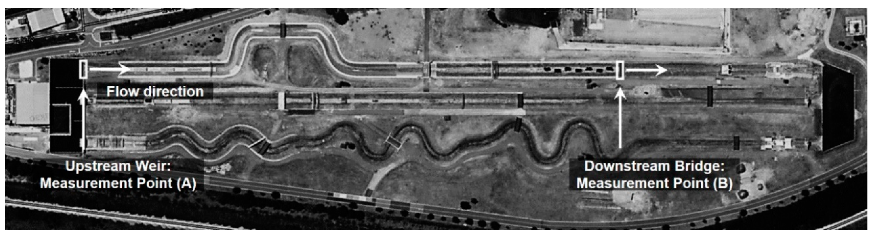
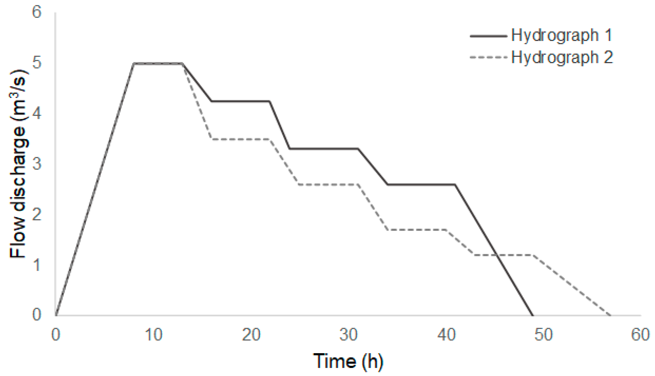
The water level data were collected in two rounds using ultrasonic sensors at a large-scale outdoor flume at the Korea Institute of Civil Engineering and Building Technology—River Experiment Center (KICT-REC) (Figure 1). The stream-scale channel’s length was 594 m, and the channel’s width was 11 m. The stream bed slope of the downstream section, which was the downstream water level measurement point, was approximately 3/1000. The generated flow in the channel could be controlled by adjusting the flow supply pump equipment. As shown in Figure 2, unsteady flow experiments with two different forms of flow discharge hydrographs were designed. While the maximum discharge of the two hydrographs was designed with the same at 5 m3/s, the total durations of the flow events were different. Two ultrasonic sensors were installed at the upstream weir of measurement point (A) and at the downstream bridge of measurement point (B) in the channel to monitor water levels when two different hydrographs were generated one after another (Figure 1). Therefore, a total of four data sets of ultrasonic sensors were collected for this study: two data sets at measurement points (A) and (B) for hydrograph 1 and two data sets at measurement points (A) and (B) for hydrograph 2. By converting the water level measured at the upstream weir of measurement point (A) to flow discharge using the previously developed relation between water level and flow discharge, changes in the flow discharge from the upstream to the channel can be tracked over time. The flow rate over a weir is a function of the head on the weir. Therefore, the flow rate measurement in a rectangular weir is based on the Bernoulli Equation principles. The discharge coefficient for a rectangular wide weir used in the experiment was determined and calibrated prior the experiments to present the rectangular wide weir equation for flow. Water level measurements at the downstream bridge of measurement point (B) observe the water level changes in the downstream section of the experimental channel.
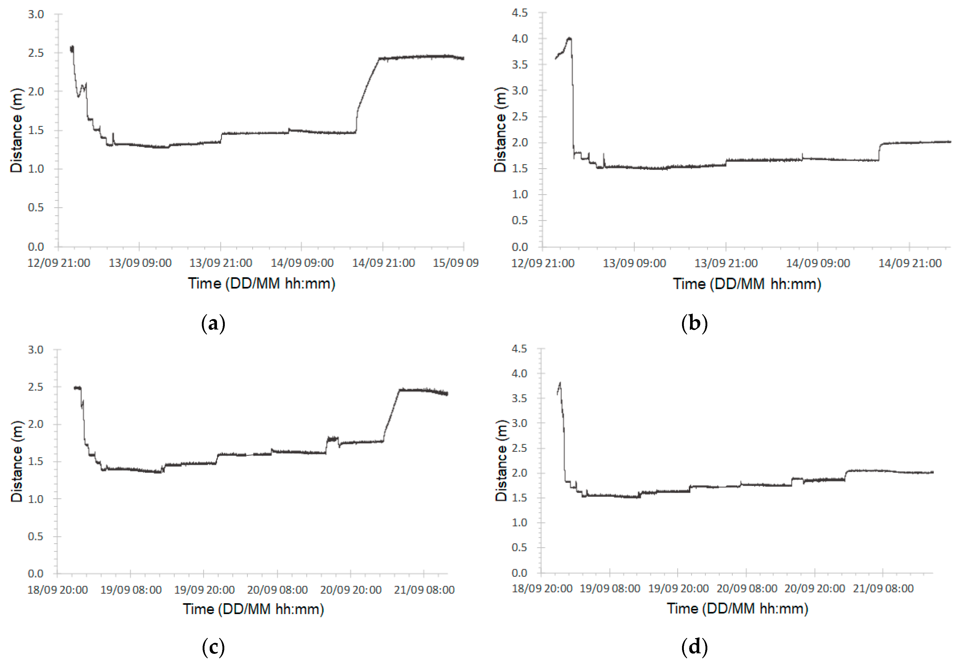
Ultrasonic sensors generate successive signals from the transmitter, and when the signals reflect off the target object’s surface and return to the receiver, their round-trip times, in conjunction with the speed of sound, are converted to distance. The ultrasonic sensors used for the water level measurements in this experiment were HC-SR04 models with a measurable distance range from the sensor unit of 0.2–4.0 m, a measurement resolution of 3 mm, and a minimum sampling interval of 60 ms. In this experiment, the raw data were sampled at intervals of 2.5 s. These sensors can be combined with data storage devices, communication modules, power supplies, level aligners, etc., according to the user’s needs [19], and in this study, the ultrasonic sensors were combined with an Arduino board and a WiFi module to collect data in real-time at the outdoor flume. The raw data acquired by this system showed the distance values from the sensor to the water surface (Figure 3). The number of data sets collected for each measurement location of the target hydrographs was between 77,040 and 96,954 (Table 1). Figure 3 shows all data, including the outliers, obtained from the ultrasonic sensor for each measurement point of the target hydrographs.
2.2. Data Processing Methods
2.2.1. Robust Statistical Methods for Outlier Detection
In water level data measured by ultrasonic sensors, outliers can occur when the ultrasonic wave is reflected before reaching the water surface, and such measurement values’ deviations can be quite large (Figure 3). Therefore, in order to detect outliers in the water level data measured by ultrasonic sensors, a robust estimator must be used that is insensitive to outliers with large deviations. According to Huber [20], Leys et al. [21], and Rousseeuw and Croux [22], the sample median can be used as a robust estimator of location because the median is very insensitive to the effects of such large deviations and can thus minimize the effect of asymmetry due to outliers in the distribution of water level data measured by ultrasonic sensors. In addition, the MAD can be used as a robust scale estimator for estimating the dispersion of data centered on the sample median. Like the median, the MAD is very insensitive to outlier deviation [20,21,22,23].
When the collected data set was given as , the MAD was defined as follows [24,25,26]:
where is a function for finding the median of the data set . Therefore, shows the median value of absolute deviations between the individual observations of data set and . In order to compare the MAD value calculated in Equation (1) with the standard deviation, Equation (2) is used to convert to the normalized MAD (MADN) [24]:
where the constant value 0.6745 is the 75% percentile of a normal distribution, which corresponds to the MAD of the standard normal distribution with a standard deviation of 1 [24,26,27,28]. The MADN(X) corresponds to the standard deviation of the normal distribution for the center location of the data estimated by the sample median.
To detect outliers, dimensionless variables must be used, as in Equation (3), to compare MADN(X) with the deviation of the individual observation centered on the location estimated by the sample median. in Equation (3) is the modified Z-score. This is compared with the outlier rejection criterion to determine if the data point is an outlier [26].
2.2.2. Exponentially Weighted Moving Average for Data Smoothing
Even if the outliers that occur in the measured water level data are entirely removed, there is approximately 2 cm of dispersion that occurs due to water waves in the flowing water. If a constant water level is repeatedly measured under the same conditions at short intervals using an ultrasonic sensor, a normal distribution is formed by the observed values due to random error, excluding outliers. Therefore, a moving average can be applied as a smoothing method. This is the simplest form of a low-pass filter that is commonly used in signal processing to smooth short-term variations in time series data. However, the actual water level can change over time during the monitoring period. Therefore the most recently observed data must be reflected more than older data in the smoothing process, and the EWMA can be used for such cases to apply lower weights to older data [29]. The EWMA exponentially reduces the weighting factors of older data as shown in Equation (4), when the data set is listed as a sequence for time [29]:
where shows the decreasing degree of weighting as a smoothing constant factor, with a range of . As shown in Equation (4), a high level of smoothing can be obtained by increasing the weight of the past data with a smaller , which makes the data dispersion smaller. However, if becomes too small, the changes in data over a short time are almost ignored. Therefore, it is necessary that vary according to the researcher’s subjective standards and the data usage purpose.
Because the EWMA requires past observations to perform calculations, the initial observation value can be problematic to establish. Therefore, some methods use the initial observation, as in , and other methods use the average of multiple initial values [29]. In this study, the initial observation has been applied for the EWMA.
2.2.3. Generalized Data Processing Algorithm for Water Levels Measured by Ultrasonic Sensors in Water Flows
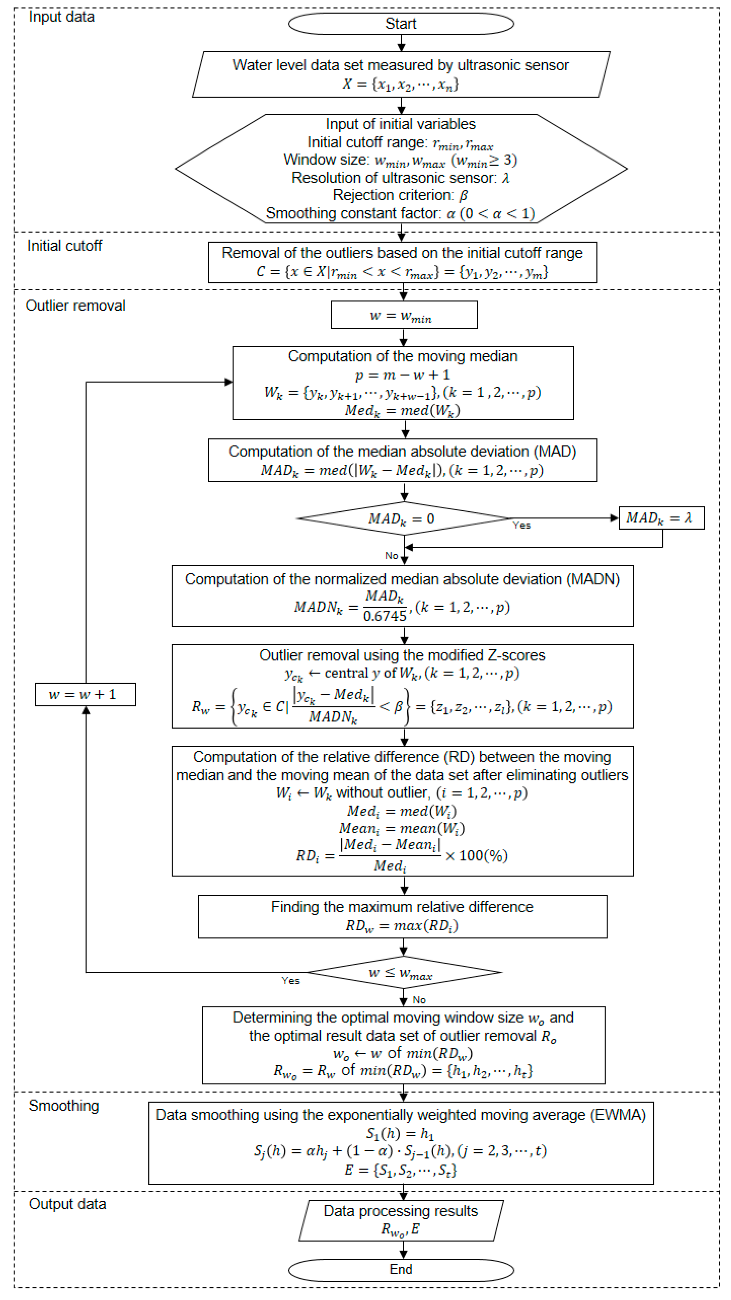
An integrated data processing algorithm for eliminating outliers and smoothing data variation in water level data collected using ultrasonic sensors was developed in this study. The proposed algorithm’s main processing steps were broadly divided into the outlier removal step and the data smoothing step (Figure 4). The outlier processing step was further divided into the initial cutoff of outliers and outlier removal using modified Z-scores. Input parameters and conditional factors such as the initial cutoff range ( and ), maximum and minimum values of window size ( and ), the smoothing constant factor (), the resolution of the ultrasonic sensor (), and the rejection criterion () must be defined by users in the data processing algorithm for water levels monitored by ultrasonic sensors. The data set after completing outlier removal () and the data set after completing both outlier removal and smoothing () were provided as the final output. The developed algorithm was coded with Python 3 to perform data processing tests on the data sets collected in the experiments.
The first step in the proposed outlier removal stage was the initial cutoff. Regarding the distance from the water surface to the ultrasonic sensor, the initial cutoff range can be determined by considering the distance from the sensor to the minimum water level, assuming that the sensor’s installation location is constant. When the minimum water level cannot be defined prior to the analysis, zero water levels can be assumed for the minimum water level. The zero water level means that there is no water flow and is the same as the bed level. In this study, data outside of this interval were determined to be clear outliers, and the proposed algorithm’s initial cutoff stage removed these outliers en masse. Therefore, when the user enters and of the initial cutoff range in this stage to define the post-processing input variables, multiple outliers outside of this interval defined as the initial cutoff range can be removed. Therefore, the number of outliers included in the raw data could be reduced, and the outlier detection performance could be improved through the sample median and MAD estimation in the next stage. If the users cannot define and of the initial cutoff range, the distance from the sensor to the bed for and the zero value for are used as a default in the algorithm.
After the initial cutoff stage, the outlier removal process was completed using modified Z-scores. This stage calculated the sample median and MAD of each data point in the dataset that passed through the initial cutoff, and then calculated the corresponding modified Z-scores, which were dimensionless values. When this value exceeded the user-entered , the corresponding data point was determined to be an outlier and removed. In this step, when the median and MAD were estimated, a moving window was applied to consider that the water level data changed over time, and therefore, the optimal window size () had to be determined. The algorithm proposed here calculated the relative difference in the moving median and the moving mean, as measures of the data set’s central tendency with outliers removed, for each window size . The that had the smallest maximum relative difference was determined to be . In order to determine ’s calculation range, input for and were needed. If the number of samples was two, the median and mean calculation results were the same. Therefore, the minimum window size had to be more than three. When the algorithm is applied to real-time monitoring system, the optimal window size cannot be determined in real time. In this case, fixed window size should be applied or optimal window size could be updated based on the previous results of data processing with a certain period of time.
If more than 50% of the values in the data set within the window size were the same values when calculating MAD during outlier removal, the calculated MAD value could become zero, and the MADN and calculations in Equations (2) and (3) would then be impossible. Machado [30], Chu et al. [31], and Vivcharuk et al. [32] have presented methods that use the mean absolute deviation (MeanAD) as an alternative to a zero MAD. However, if all data within the window size have the same value, MeanAD would also be zero. Even in cases where MeanAD was not zero, if there were outliers with large deviations, the estimated scale would be large, and detecting outliers with relatively small deviations would be difficult. When measuring the water level of flowing water, cases often occur where the MAD and MeanAD values are zero in situations where the water level remains constant. Therefore, in this study, to resolve this problem, the minimum measurement unit of the ultrasonic sensor was entered by the user as input data. Therefore, a method was used to define the resolution as the MAD value when the calculated MAD was zero. Because was the same as the deviation of the minimum unit that can occur during measurement, it corresponded to the minimum size of MAD that could occur when MAD was not zero. This processing method minimized the effect of outliers with relatively large deviations when more than 50% of the values of the data set in the window size had the same value, and could thus detect outliers robustly.
Finally, the EMWA data smoothing stage minimized the dispersion of data due to random errors in the water level data from which outliers had been completely removed. This step used Equation (4) on , which is the output data after the outliers were removed. The initial stage of the algorithm for this step required a smoothing constant input, for which different values could be used according to the situation as explained in Section 2.2.2. In this study, the water level data measured by ultrasonic sensors was used to evaluate the data’s level of smoothing according to the smoothing constant (), and the results are presented in Section 3.
3. Results
3.1. Outlier Removal Processing
The algorithm developed to remove outliers and smooth the water level data collected by ultrasonic sensors was applied to the water level data acquired by the stream-scale experiments described in Section 2. The input variables and required for the initial cutoff stage were set at 2.6 m and 1.2 m, respectively, for the data set acquired at the downstream bridge, and 4.1 m and 1.3 m, respectively, for the data set acquired at the upstream weir. Table 1 shows the number of outliers that were removed by the initial cutoff process. Because the outlier distribution characteristics in each data set were different, the ratios of outliers removed by the initial cutoff were different.
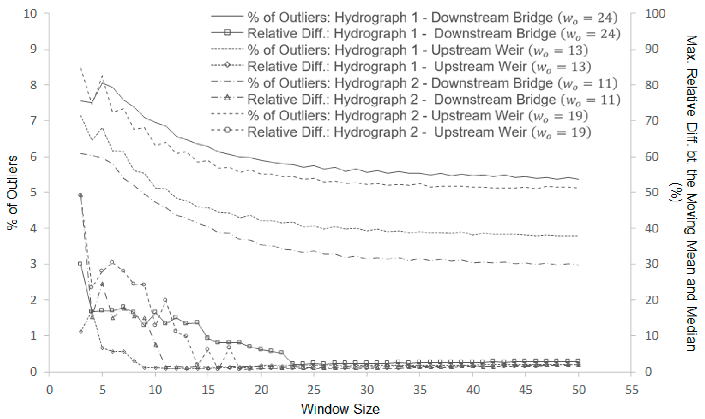
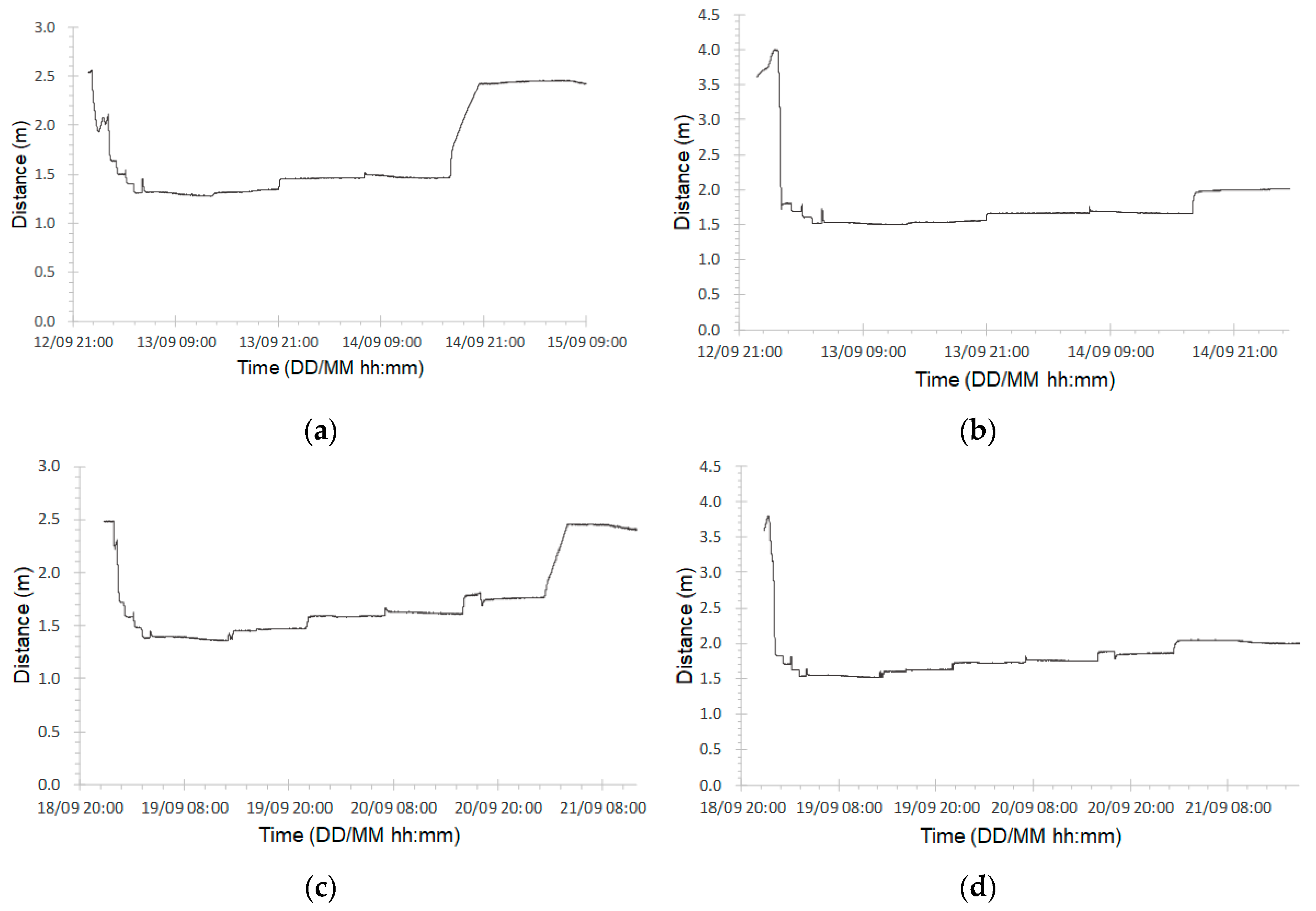
Further outlier removal was performed by calculating modified Z-scores for data sets that passed through the initial cutoff stage. Here, the 0.003 m resolution of the experiment’s ultrasonic sensors which was provided by the manufacture was used as to handle cases in which the MAD value was zero. For the modified Z-scores’ rejection criterion , a value of 3.5 was used, following the standard proposed by Iglewicz and Hoaglin (1993). To calculate the optimal window size for removing outliers, 3 and 50 were used for and , respectively. The window size was increased by 1, and the maximum value of the relative difference between the moving median and moving mean was calculated for the data set with outliers removed for each of a total of 48 window sizes. Figure 5 shows the maximum relative difference between the moving median and mean and the outlier detection ratios for the 48 window sizes. Because the optimal window size was set as the window size with the minimum value that included the maximum relative differences between the moving median and mean, the optimal window sizes for the four data sets ranged between 11 and 24. The ratio of detected outliers according to the increase in window size showed a trend of exponential decrease. The maximum relative difference decreased as the window size increased and then increased slightly after the lowest value. When was set too small, cases occurred where there was a low ratio of normal values in the data sample, and the estimation accuracy of the moving median and MAD decreased, whereas the ratio of inaccurate outlier detections increased. Finally, Figure 6 shows the data set that passed the outlier removal process. The ratio of data detected as outliers in the raw data set was at least 14.4% and at most 30.6% (Table 1). Furthermore, more than 70% of all outliers were removed in the initial cutoff stage.
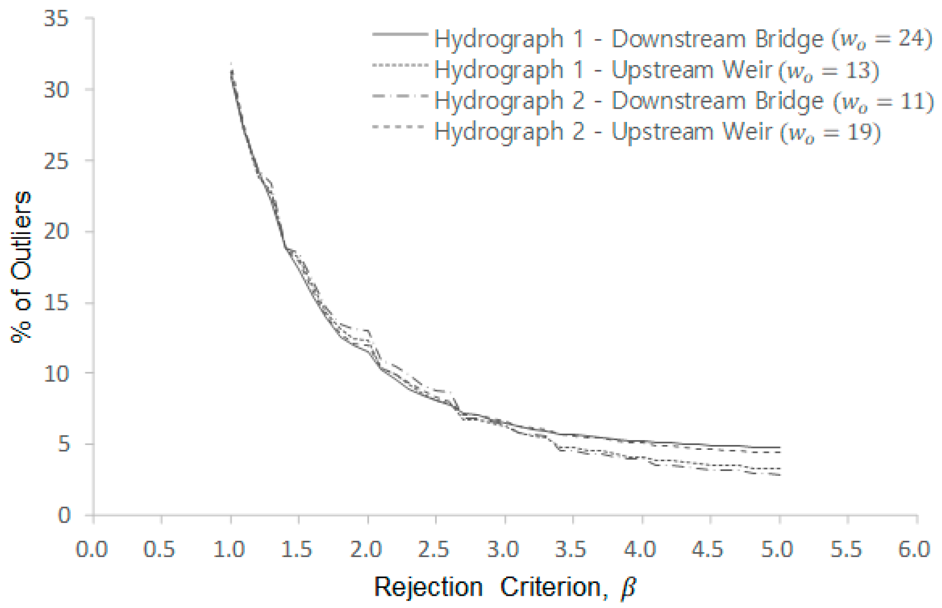
In addition to the window size setting, this study also analyzed the degree of outlier detection according to changes in the rejection criterion that the user must enter as an input value in the outlier stage using modified Z-scores. While the value of 3.5 that was proposed by Iglewicz and Hoaglin [26] is commonly used, a sensitivity analysis for the rejection criterion is required to ensure that the value of 3.5 is appropriate for outlier detection of water level data measured by ultrasonic sensors. In this study, was increased from 1 to 5 in units of 0.1, and the corresponding ratios of removed outliers were calculated; the results are shown in Figure 7. For the window size used to calculate the moving median and MAD, the optimal window size found when was set at 3.5 was used. As shown in Figure 7, when increased, the ratio of removed data decreased exponentially, and when exceeded the range from 3.0 to 3.5, the percentage reduction in removed outliers was greatly reduced. Table 2 shows the ratios of removed outliers when different rejection criteria were applied to the four data sets.
3.2. Data Smoothing
The ultrasonic sensor-acquired water level data with the outliers removed exhibited approximately 2 cm of data dispersion due to random error. To mitigate this data dispersion, data smoothing using EWMA was performed in the algorithm’s final stage. Figure 8 shows the data smoothing results when the smoothing constant factor was set at 0.1. The dispersion in the water level data due to random error was reduced.
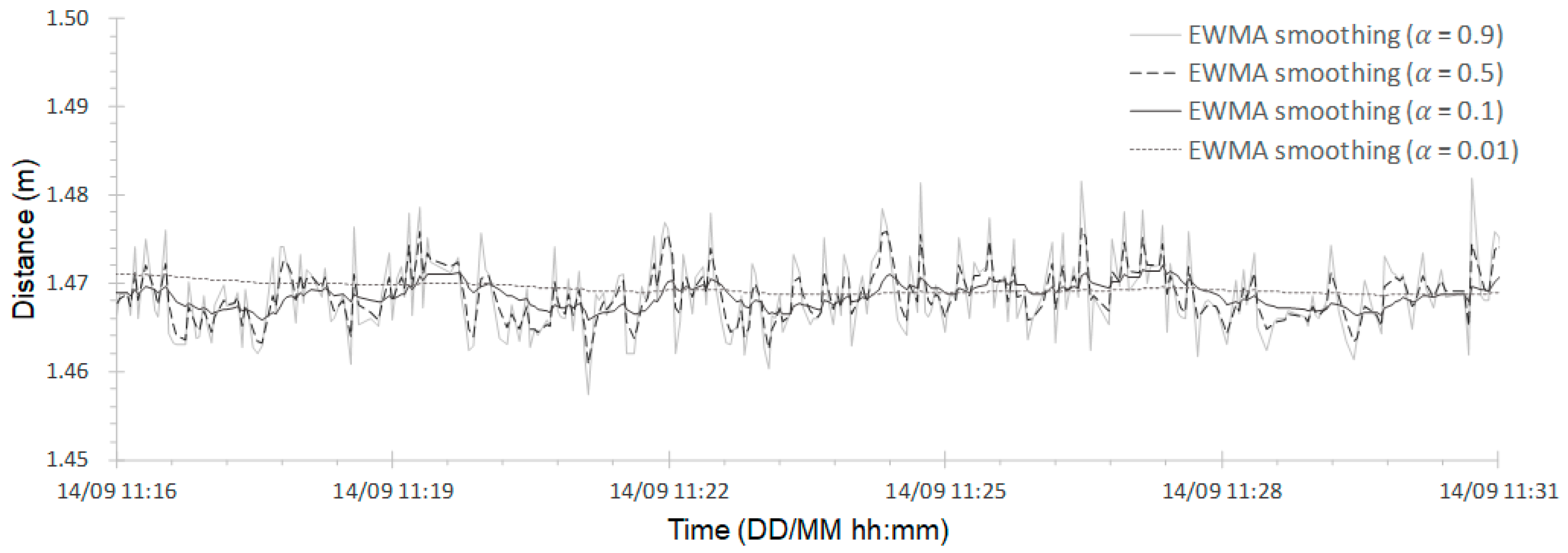
These smoothing process results can vary according to the smoothing constant factor . Figure 9 compares the smoothing process effects on a partial section of the overall data when was 0.01, 0.1, 0.5, and 0.9. When was 0.01, the weight of the previous data increased and the water level data’s dispersion was greatly reduced, although short-term changes in the data were ignored. When had a large value of 0.5 or more, the data’s dispersion was reflected very closely, although the smoothing effect was greatly reduced, contrary to the goal of this study’s smoothing process. Thus, the smoothing effect based on EWMA was very sensitive to . In order to quantitatively examine the smoothing effect according to the input variable , the changes in the standard deviation according to were calculated for the data set in Figure 9 (Table 3). When was 1, the weight of the previous data in Equation (4) became zero, reflecting a case where there was no smoothing process effect. Therefore, the level of smoothing was calculated by a standard deviation reduction rate based on the standard deviation of 0.047 when was 1 which represent. The smoothing effect on the water level data increased as decreased.
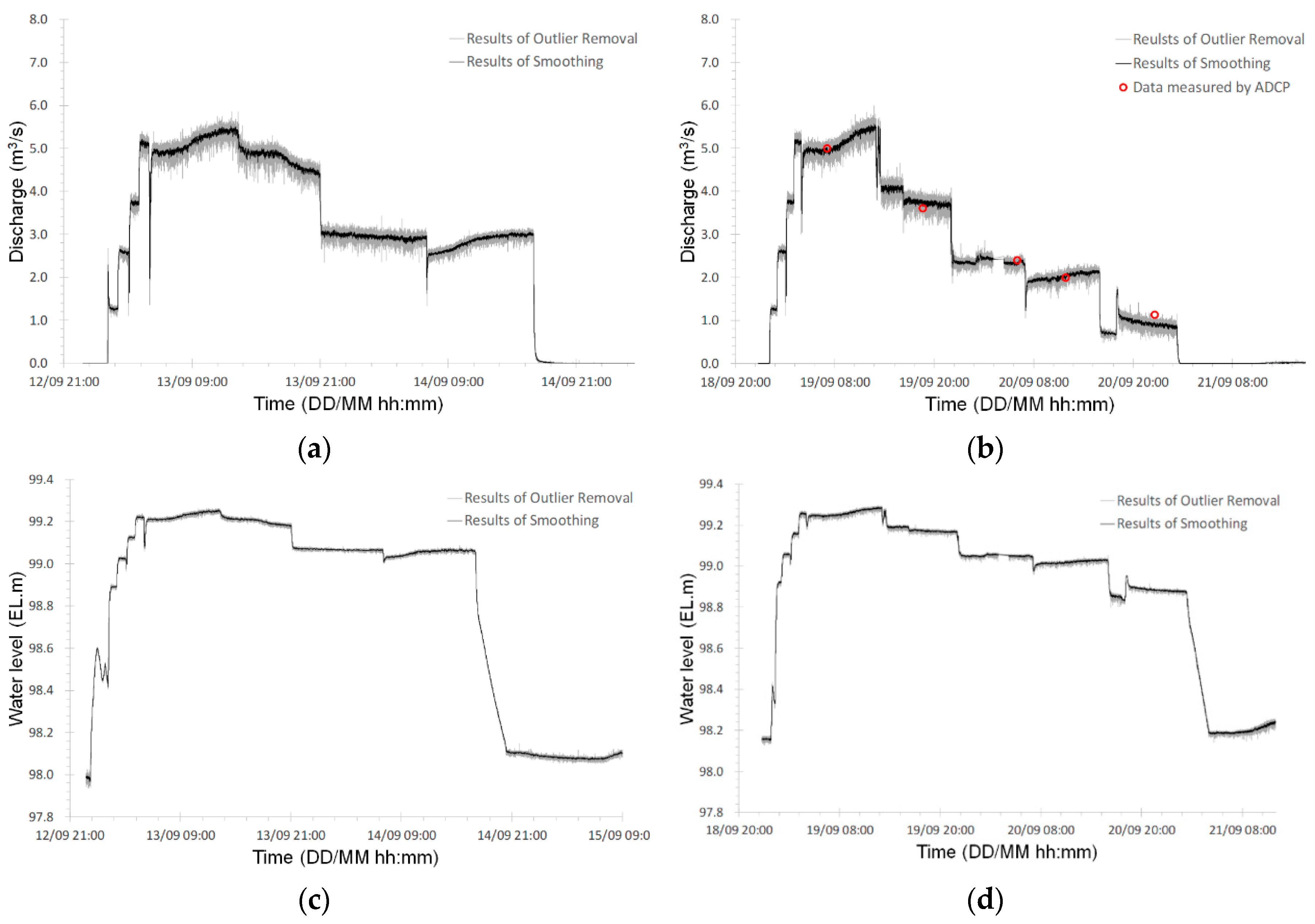
Finally, Figure 10 shows the results when the data set with complete outlier removal and the EWMA-smoothed data set were both converted to flow discharge and water level. Figure 10a,b show the results when the distance from the ultrasonic sensor to the water surface in the upstream weir reservoir was converted to a water level value and then converted into flow discharge by the weir equation describing the relation between water stage and flow discharge. That is, Figure 10a,b recreate Figure 2′s target discharge hydrographs 1 and 2. Flow discharge in Figure 10b for hydrograph 2 was validated through cross-verification from the discharge data measured by ADCP (Acoustic Doppler Current Profiler) in the experiment. ADCP is a hydroacoustic current meter to measure current velocities over a depth range and to produce flow discharge data. During the experiment of hydrograph 2, ADCP was applied to get the information for flow rate in the channel section and the results were compared in Figure 10b with the data of flow discharge converted from water levels measured by ultrasonic sensors in the upstream weir reservoir. ADCP measurement performed each eight times for five different steps of hydrograph 2 and the results were produced by averaging eight-time measurements. For the comparison, flow discharge data produced by ultrasonic sensor was averaged for the same period corresponding to eight-time measurements of ADCP for each step of hydrograph 2. The deviations from flow discharges measured by ADCP were −0.05 m3/s, +0.14 m3/s, −0.06 m3/s, +0.07 m3/s, and −0.23 m3/s followed by time sequence. Except the lowest flow condition, the deviations of flow discharge converted by water levels measured by ultrasonic sensors range from −2.17% to 3.81% of flow discharges measured by ADCP.
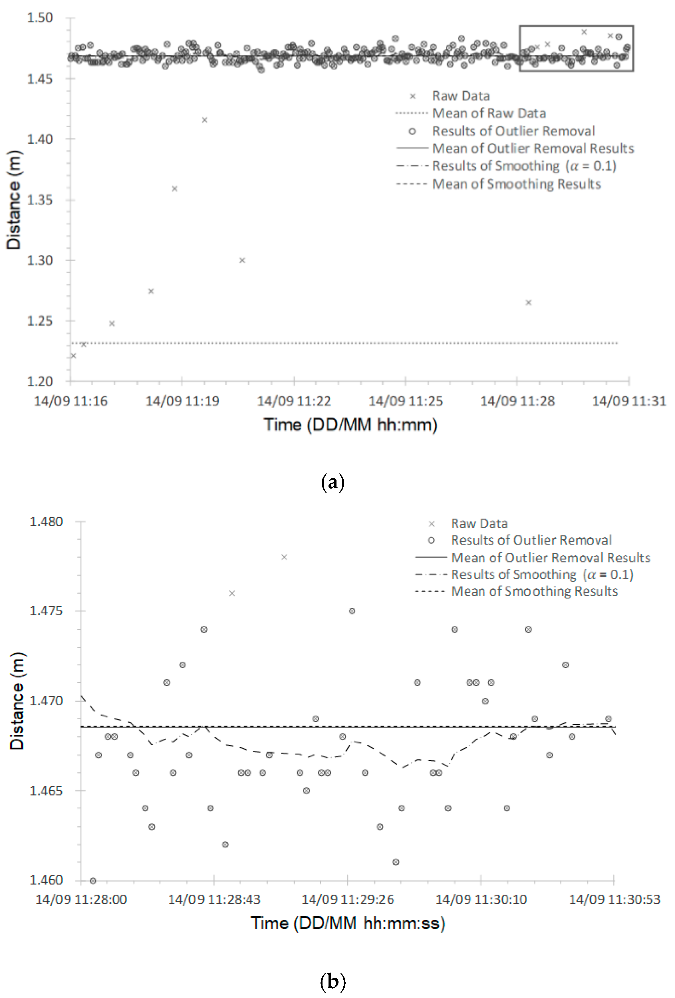
Figure 10a,b show the very large difference in the degree of dispersion in the data that had undergone outlier removal and the data that had undergone the smoothing process. Furthermore, when the flow was large, this difference was even larger. In order to compare the data processing results by stage, Figure 11 shows the interval data from 14/09 11:16 to 14/09 11:31 in the hydrograph 1—downstream bridge data set, which included the data on the distance from the ultrasonic sensor to the water surface that had not been converted to water level data. The average values of the outlier removal and smoothing results for this interval were almost the same at 1.46855 m and 1.46860 m, respectively. However, the average value for raw data without data processing was 1.232 m, demonstrating the difference due to unremoved outliers.
4. Discussion and Conclusions
This study developed an outlier removal and smoothing process algorithm for water level data collected using ultrasonic sensors in a stream-scale experiment. The study included sensitivity analyses on factors that were subjectively determined by the user in each data processing step, including the window size for the MAD of outlier detection, the rejection criterion for modified Z-scores of outlier removal, and the smoothing constant for the EWMA.
In the water level data set that was collected by the ultrasonic sensors in this study, there were many outliers with relatively large deviations distributed in the set and a relatively large random error due to the occurrence of water waves. Considering these data characteristics, the data processing algorithm developed in this study was broadly divided into an outlier removal process and a smoothing process. The algorithm incorporated an initial cutoff stage that set the initial cutoff range and determined that data outside this interval were outliers, removing them en masse. This process detected over 70% of all outliers in the water level data set captured by ultrasonic sensors. The outlier removal process after the initial cutoff used modified Z-scores based on the median and MAD. The outlier removal stage included a process for determining the optimal window size for setting the moving median and MAD. To address cases when the MAD was zero, such as when the same value was distributed above a specific ratio in the data set for the given window size, the proposed algorithm defined the ultrasonic sensors’ resolution as the MAD value. EWMA was then used in the data smoothing process, which allowed different levels of smoothing results to be calculated according to the data processing goals by entering various values for the smoothing constant factor .
Regarding the sensitivity analysis of the algorithm, the optimal window size for the outlier removal process was determined based on the maximum relative difference between the moving median and moving mean after outlier removal, which was used as the evaluation standard for the measure of central tendency. When the window size was small, the number of detected outliers was higher, and the estimation accuracy of the sample median and MAD were reduced, resulting in a higher rate of inaccurate outlier detection in the modified Z-score stage. The ratio of removed outliers decreased exponentially as the window size increased. The maximum relative difference between moving median and moving mean after outlier removal decreased as until a fixed level, and then increased slightly after the lowest level. was the rejection criterion for the modified Z-scores, which the algorithm used to remove outliers, and as its value increased, the ratio of detected outliers tended to decrease exponentially. If exceeded the range from 3.0 to 3.5, the percentage decrease in removed outliers was greatly reduced. Finally, the level of smoothing by EWMA in the smoothing process was expressed as the rate of reduction in the standard deviation caused by a reduction in , based on the standard deviation value when the smoothing constant factor was 1.0. This study confirmed that the level of smoothing for water level data measured by ultrasonic sensors increased to a maximum 84.9% of standard deviation reduction as the smoothing constant factor decreased.
Author Contributions
Conceptualization, I.B. and U.J.; Methodology, I.B. and U.J.; Software, I.B.; Formal Analysis, I.B. and U.J.; Investigation, I.B. and U.J.; Data Curation, I.B. and U.J.; Writing—original draft preparation, I.H.; Writing—review and editing, U.J.; Supervision, U.J.; Project administration, U.J.; Funding acquisition, U.J.
Funding
This research was supported by Korea Institute of Civil Engineering and Building Technology (KICT) for the International Matching Joint Research Project, grant number 20180561, and KICT-REC (River Experiment Center) for REC International Experiment Days (RIED) 2017.
Acknowledgments
The authors gratefully acknowledge the support of all participants of KICT, CER (Center for Ecohydraulics Research) at the University of Idaho, Nature and Technology, and TENELEVEN.
Conflicts of Interest
The authors declare no conflict of interest.
References
- Herschy, R.W. Streamflow Measurement; CRC Press: Boca Raton, FL, USA, 2014. [Google Scholar]
- Fenton, J.D.; Keller, R.J. The Calculation of Streamflow from Measurements of Stage, Technical Report 01/6; CRC for Catchment Hydrology: Canberra, Australia, 2001. [Google Scholar]
- Boiten, W. Hydrometry: IHE Delft Lecture Note Series, UNESCO-IHE Lecture Note Series; 3rd ed.; Taylor & Francis: Leiden, The Netherlands, 2008; p. 247. [Google Scholar]
- Sauer, V.B.; Turnipseed, D.P. Stage Measurement at Gaging Stations. In U.S. Geological Survey Techniques and Methods 3-A7; U.S. Geological Survey: Reston, VA, USA, 2010; p. 45. [Google Scholar] [CrossRef]
- World Meteorological Organization. Volume I—Fieldwork. WMO-No. 1044. In Manual on Stream Gauging; WMO: Geneva, Switzerland, 2010; p. 250. [Google Scholar] [CrossRef]
- Mcmillan, H.; Krueger, T.; Freer, J. Benchmarking observational uncertainties for hydrology: Rainfall, river discharge and water quality. Hydrol. Process. 2012, 26, 4078–4111. [Google Scholar] [CrossRef]
- Horner, I.; Renard, B.; Le Coz, J.; Branger, F.; McMillan, H.K.; Pierrefeu, G. Impact of Stage Measurement Errors on Streamflow Uncertainty. Water Resour. Res. 2018, 54, 1952–1976. [Google Scholar] [CrossRef]
- Hamilton, A.S.; Moore, R.D. Quantifying Uncertainty in Streamflow Records. Can. Water Resour. J. 2012, 37, 3–21. [Google Scholar] [CrossRef]
- Kruger, A.; Krajewski, W.F.; Niemeier, J.J.; Ceynar, D.L.; Goska, R. Bridge-mounted river stage sensors (BMRSS). IEEE Access 2016, 4, 8948–8966. [Google Scholar] [CrossRef]
- Mousa, M.; Zhang, X.; Claudel, C. Flash Flood Detection in Urban Cities Using Ultrasonic and Infrared Sensors. IEEE Sens. J. 2016, 16, 7204–7216. [Google Scholar] [CrossRef]
- Rahmtalla, A.; Mohamed, A.; Wei, W.G. Real Time Wireless Flood Monitoring System Using Ultrasonic Waves. Int. J. Sci. Res. 2014, 3, 2012–2015. [Google Scholar]
- Satria, D.; Yana, S.; Munadi, R.; Syahreza, S. Prototype of Google Maps-Based Flood Monitoring System Using Arduino and GSM Module. Int. Res. J. Eng. Technol. 2017, 4, 1044–1047. [Google Scholar]
- Sunkpho, J.; Ootamakorn, C. Real-time flood monitoring and warning system. Songklanakarin J. Sci. Technol. 2011, 33, 227–235. [Google Scholar]
- Bae, I.; Yu, K.; Yoon, B.; Kim, S. A study on the applicability of invisible environment of surface image velocimeter using far infrared camera. J. Korea Water Resour. Assoc. 2017, 50, 597–607. (In Korean) [Google Scholar] [CrossRef]
- Clemmens, A.J.; Wahl, T.L.; Bos, M.G.; Replogle, J.A. Water Measurement with Flumes and Weirs; International Institute for Land Reclamation and Impovement: Wageningen, The Netherlands, 2001; p. 382. [Google Scholar]
- Cho, H.; Jeong, S.T.; Ko, D.H.; Son, K.-P. Efficient Outlier Detection of the Water Temperature Monitoring Data. J. Korean Soc. Coast. Ocean Eng. 2014, 26, 285–291. (In Korean) [Google Scholar] [CrossRef]
- National Disaster Management Research Institute (NDMRI). Small River Facilities Standard Improvement Experiment and Flow Measurement Technology Development; National Disaster Management Research Institute: Jungang-dong, Korea, 2017. (In Korean)
- International Organization for Standardization. ISO 772:2011 Hydrometry—Vocabulary and Symbols, 5th ed.; International Organization for Standardization: Geneva, Switzerland, 2011. [Google Scholar]
- Madli, R.; Hebbar, S.; Pattar, P.; Golla, V. Automatic detection and notification of potholes and humps on roads to aid drivers. IEEE Sens. J. 2015, 15, 4313–4318. [Google Scholar] [CrossRef]
- Huber, P.J. Robust Statistics; Wiley: Hoboken, NJ, USA, 1981. [Google Scholar] [CrossRef]
- Leys, C.; Ley, C.; Klein, O.; Bernard, P.; Licata, L. Detecting outliers: Do not use standard deviation around the mean, use absolute deviation around the median. J. Exp. Soc. Psychol. 2013, 49, 764–766. [Google Scholar] [CrossRef] [Green Version]
- Rousseeuw, P.J.; Croux, C. Alternatives to the median absolute deviation. J. Am. Stat. Assoc. 1993, 88, 1273–1283. [Google Scholar] [CrossRef]
- Croux, C.; Filzmoser, P.; Oliveira, M.R. Algorithms for Projection-Pursuit robust principal component analysis. Chemom. Intell. Lab. Syst. 2007, 87, 218–225. [Google Scholar] [CrossRef]
- Maronna, R.A.; Martin, D.R.; Yohai, V.J. Robust Statistics: Theory and Methods; Wiley: Hoboken, NJ, USA, 2006. [Google Scholar]
- Huber, P.J. Robust statistics. In International Encyclopedia of Statistical Science; Springer: Berlin, Germany, 2011; pp. 1248–1251. [Google Scholar]
- Iglewicz, B.; Hoaglin, D.C. How to Detect and Handle Outliers; Asq Press: Milwaukee, WI, USA, 1993; p. 87. [Google Scholar]
- Satake, E. Statistical Methods and Reasoning for the Clinical Sciences: Evidence-Based Practice; Plural Publishing: Austin, TX, USA, 2014. [Google Scholar]
- Huxley, T.H. Outing the Outliers–Tails of the Unexpected. In Proceedings of the ICEAA 2016 International Training Symposium, Bristol, UK, 17–20 October 2016. [Google Scholar]
- Brown, R.G. Smoothing, Forecasting and Prediction of Discrete Time Series; Prentice-Hall international series in management; Prentice-Hall: Upper Saddle River, NJ, USA, 1963. [Google Scholar]
- Machado, J.M.O. Outlier Detection in Accounting Data. Master’s Thesis, University of Porto, Porto, Portugal, 2018. [Google Scholar]
- Chu, J.Y.; Shyr, J.-Y.; Zhong, W. Decision Tree Insight Dsicovery. U.S. Patent 2014/0279775 A1, 18 September 2014. [Google Scholar]
- Vivcharuk, V.; Baardsnes, J.; Deprez, C.; Sulea, T.; Jaramillo, M.; Corbeil, C.R.; Mullick, A.; Magoon, J.; Marcil, A.; Durocher, Y.; et al. Assisted Design of Antibody and Protein Therapeutics (ADAPT). PLoS ONE 2017, 12, e0181490. [Google Scholar] [CrossRef] [PubMed]
Figure 1.
Stream-scale experiment channel of Korea Institute of Civil Engineering and Building Technology—River Experiment Center (KICT-REC).
Figure 1.
Stream-scale experiment channel of Korea Institute of Civil Engineering and Building Technology—River Experiment Center (KICT-REC).

Figure 2.
Target hydrographs designed for this study in the stream-scale experiment channel.

Figure 3.
Measured raw data of the distance from the ultrasonic sensor to water surface for about 60 h. (a) Case of hydrograph 1—downstream bridge; (b) case of hydrograph 1—upstream weir; (c) case of hydrograph 2—downstream bridge; (d) case of hydrograph 2—upstream weir.
Figure 3.
Measured raw data of the distance from the ultrasonic sensor to water surface for about 60 h. (a) Case of hydrograph 1—downstream bridge; (b) case of hydrograph 1—upstream weir; (c) case of hydrograph 2—downstream bridge; (d) case of hydrograph 2—upstream weir.

Figure 4.
Flow chart of data processing for the outlier removal and the data smoothing for water level data measured by ultrasonic sensor.
Figure 4.
Flow chart of data processing for the outlier removal and the data smoothing for water level data measured by ultrasonic sensor.

Figure 5.
Outlier detection rate and maximum relative difference between the moving mean and median according to window size.
Figure 5.
Outlier detection rate and maximum relative difference between the moving mean and median according to window size.

Figure 6.
Final data set after the outlier removal process. (a) Case of hydrograph 1—downstream bridge; (b) case of hydrograph 1—upstream weir; (c) case of hydrograph 2—downstream bridge; (d) case of hydrograph 2—upstream weir.
Figure 6.
Final data set after the outlier removal process. (a) Case of hydrograph 1—downstream bridge; (b) case of hydrograph 1—upstream weir; (c) case of hydrograph 2—downstream bridge; (d) case of hydrograph 2—upstream weir.

Figure 7.
Relations between outlier percentage and rejection criterion.

Figure 8.
The data set after the smoothing process using EWMA. (a) Case of hydrograph 1—downstream bridge; (b) case of hydrograph 1—upstream weir; (c) case of hydrograph 2—downstream bridge; (d) case of hydrograph 2—upstream weir.
Figure 8.
The data set after the smoothing process using EWMA. (a) Case of hydrograph 1—downstream bridge; (b) case of hydrograph 1—upstream weir; (c) case of hydrograph 2—downstream bridge; (d) case of hydrograph 2—upstream weir.

Figure 9.
Comparison of the smoothing levels with different smoothing constant factors (case of hydrograph 1—downstream bridge).
Figure 9.
Comparison of the smoothing levels with different smoothing constant factors (case of hydrograph 1—downstream bridge).

Figure 10.
Flow discharge in the upstream weir and water level in the downstream bridge monitored by ultrasonic sensors. (a) Flow discharge converted by water level data in case of hydrograph 1—upstream weir; (b) flow discharge converted by water level data in case of hydrograph 2—upstream weir; (c) water level converted by measured data in case of hydrograph 1—downstream bridge; (d) water level converted by measured data in case of hydrograph 2—downstream bridge.

Figure 11.
Comparison of raw data, outlier removal result, and smoothing result of water level data measured by ultrasonic sensor in downstream bridge for hydrograph 1. (a) Comparison section from 14/09 11:16 to 14/09 11:31; (b) comparison section from 14/09 11:28 to 14/09 11:31.
Figure 11.
Comparison of raw data, outlier removal result, and smoothing result of water level data measured by ultrasonic sensor in downstream bridge for hydrograph 1. (a) Comparison section from 14/09 11:16 to 14/09 11:31; (b) comparison section from 14/09 11:28 to 14/09 11:31.


Table 1.
Results of outlier detection for each data set and moving window size for median absolute deviation (MAD) process.
Table 1.
Results of outlier detection for each data set and moving window size for median absolute deviation (MAD) process.
| Flow Condition | Sensor Location | Acquisition Time (h) | Optimal Moving Window Size | Number of Raw Data | Number of Outliers Removed with Cutoff | Number of Outliers Removed with MAD | Total Outlier | % of Outlier | Number of Data after Outlier Removal |
|---|---|---|---|---|---|---|---|---|---|
| Hydrograph 1 | Downstream bridge | 58 | 24 | 86,942 | 22,971 | 3653 | 26,624 | 30.6 | 60,318 |
| Hydrograph 1 | Upstream weir | 52 | 13 | 77,040 | 10,674 | 3169 | 13,843 | 18.0 | 63,197 |
| Hydrograph 2 | Downstream bridge | 61 | 11 | 87,916 | 9087 | 3601 | 12,688 | 14.4 | 75,228 |
| Hydrograph 2 | Upstream weir | 67 | 19 | 96,954 | 12,650 | 4748 | 17,398 | 17.9 | 79,556 |
Table 2.
Percentage of detected outliers according to rejection criterion.
| Rejection Criterion | % of Outliers | |||
|---|---|---|---|---|
| Case of Hydrograph 1 | Case of Hydrograph 2 | |||
| Downstream Bridge | Upstream Weir | Downstream Bridge | Upstream Weir | |
| 1.0 | 30.92 | 31.32 | 31.22 | 31.83 |
| 2.0 | 11.56 | 13.04 | 12.29 | 11.99 |
| 2.5 | 8.05 | 8.77 | 8.13 | 8.31 |
| 3.0 | 6.52 | 6.37 | 6.23 | 6.60 |
| 3.5 | 5.71 | 4.57 | 4.78 | 5.63 |
| 4.0 | 5.25 | 3.95 | 4.15 | 5.12 |
| 5.0 | 4.76 | 2.87 | 3.28 | 4.42 |
Table 3.
Level of smoothing and standard deviation with different smoothing constant factors (used data set from 14/09 11:16 to 14/09 11:31 of case of hydrograph 1—downstream bridge).
Table 3.
Level of smoothing and standard deviation with different smoothing constant factors (used data set from 14/09 11:16 to 14/09 11:31 of case of hydrograph 1—downstream bridge).
| Smoothing Constant Factor | Standard Deviation (m) | Level of Smoothing (%) |
|---|---|---|
| 1.00 | 0.0047 | 0.0 |
| 0.90 | 0.0043 | 9.3 |
| 0.80 | 0.0039 | 17.6 |
| 0.70 | 0.0035 | 25.3 |
| 0.60 | 0.0032 | 32.5 |
| 0.50 | 0.0028 | 39.4 |
| 0.40 | 0.0025 | 46.1 |
| 0.30 | 0.0022 | 53.0 |
| 0.20 | 0.0019 | 60.5 |
| 0.10 | 0.0014 | 70.6 |
| 0.01 | 0.0007 | 84.9 |
© 2019 by the authors. Licensee MDPI, Basel, Switzerland. This article is an open access article distributed under the terms and conditions of the Creative Commons Attribution (CC BY) license (http://creativecommons.org/licenses/by/4.0/).
Share and Cite
MDPI and ACS Style
Bae, I.; Ji, U. Outlier Detection and Smoothing Process for Water Level Data Measured by Ultrasonic Sensor in Stream Flows. Water 2019, 11, 951. https://doi.org/10.3390/w11050951
AMA Style
Bae I, Ji U. Outlier Detection and Smoothing Process for Water Level Data Measured by Ultrasonic Sensor in Stream Flows. Water. 2019; 11(5):951. https://doi.org/10.3390/w11050951
Chicago/Turabian StyleBae, Inhyeok, and Un Ji. 2019. "Outlier Detection and Smoothing Process for Water Level Data Measured by Ultrasonic Sensor in Stream Flows" Water 11, no. 5: 951. https://doi.org/10.3390/w11050951
Note that from the first issue of 2016, this journal uses article numbers instead of page numbers. See further details here.