The Influence of Temperature on the Bulk Settling of Cohesive Sediment in Still Water with the Lattice Boltzmann Method

Abstract

Flocculation is very common and significant for cohesive sediment in coastal areas, and the influence of temperature on it cannot be neglected. The Lattice Boltzmann Method (LBM), combined with the extended Derjaguin‒Landau‒Verwey‒Overbeek (XDLVO) theory, which considers the micro-interaction forces between particles, was applied to simulate the settling and flocculation processes of cohesive sediment under various temperature conditions. The floc size, floc volume, suspended sediment concentration (SSC), and settling velocities were analyzed. The analyses revealed that with increasing temperature, both the mean floc diameter and floc volume grew, while the maximum floc diameter initially increased and then slightly decreased with its peak at 10 °C. During settling, the SSC change rate was exponentially related to the SSC, with an optimal fitting index of 0.3. The LBM sediment settling velocity was also compared with some formulas and physical model tests; the comparison results consistently demonstrated that the LBM was reasonable for modeling the bulk settling of cohesive sediment. Further discussions illustrated that the cohesive sediment is more difficult to flocculate at low temperatures due to the low aggregation frequency, while at high temperatures, some large flocs broke easily due to the effect of the short-distance force and macro force.

1. Introduction

Cohesive sediment is an important type of sediment in the near shore zone. As a result of its own physical properties and external environments, cohesive sediment can form flocs easily. Temperature is one of many factors that influence flocculation [1,2,3]. Particularly in middle- and high-latitude areas, the water temperature varies drastically: it may be close to 0 °C in winter and exceed 30 °C in summer [4,5,6,7].

Thus far, much research has been conducted to study the influence of temperature on cohesive sediment. Lau [8] studied temperature’s effects on the settling velocity and deposition of cohesive sediment in an annular channel of distilled water that was housed in a temperature-controlled chamber. He claimed that, as temperature increased, the repulsive forces between particles increased while attractive forces remained the same, which resulted in a lower degree of deposition and a smaller effective settling velocity. However, his results were completely opposite to the still water experimental conclusions of Owen [9], whose test was conducted in a settling tube in still water, and showed that the influence of temperature on water viscosity was the main cause for sediment velocity variation. Jiang et al. [4] conducted a few indoor cylinder tests in flowing water, salt water and quiescent water, with clay samples (mean diameter of 17 μm) taken from the Changjiang Estuary, to study the influence of temperature on mud particle deposition and flocculation. Jiang’s study results supported the viewpoint that temperature was the major influencing factor on mud deposition. For water temperatures less than 25 °C, the deposition was limited as particles were preferentially deposited as single grains, while when it exceeded 25 °C, flocculation occurred, and the settling rate increased rapidly. Wan et al. [6] conducted some tests in temperature-controllable and autostirring settling columns, and the results revealed that increasing the temperature had a positive effect on floc velocity, and the velocity with higher suspended sediment concentration (SSC) was much greater than that with lower SSC, whereas this impact was negligible when the SSC was over 8 g/L.

Other studies on this subject via field observations have also been conducted and were mainly reflected by the day‒night or seasonal variation [7,10,11,12,13]. Most of the studies deemed that the temperature affected the sediment properties of settling, aggregation, or deposition through changing the organism. Dickhudt [7] measured the sediment erodibility in York River from April 2006 to October 2007, where the erodibility was low in summer and fall and high in winter and spring, with the highest erosion rate in May. Lee et al. [10] analyzed some clay with a primary size of approximately 3 μm along the Belgian coastal zone and revealed that a low turbulent shear and/or temperature increase concurred with increasing median diameters. Andersen and Pejrup [11] observed a marked seasonality with respect to equivalent settling diameter in situ at the Lister Dyb tidal area of Kongsmark, Denmark. They found that small diameters were observed during winter and early spring, whereas higher values were seen in other seasons. Xia et al. [12] sampled suspended sediment in the Pearl River Estuary, China in January and July, and in their experiments the settling velocities and effective densities differed extensively between the two seasons. Guo and He [13] also focused on in situ suspended sediment flocculation in the Yangtze River, and their results showed some differences in settling velocities owing to temperature but could not avoid other factors such as salinity and SSC.

In addition, several researchers [14,15] have studied the temperature effect through theoretical analysis. They can be summarized into two main viewpoints: One explanation was that the rising temperature weakened the short-distance force between particles; and the other held a viewpoint that the temperature mainly effected flocculation via water viscosity, that is, the increase in temperature decreases the water viscosity (1.00 × 10⁻⁶ m² s⁻¹ at 20 °C, 1.31 × 10⁻⁶ m² s⁻¹ at 10 °C and 0.80 × 10⁻⁶ m² s⁻¹ at 30 °C) and accelerates the sediment settling velocity according to Stokes’s Law [9,15]. Most properties of the flocculation process can usually be deduced from the flocs’ size and their effective density. With the increasing development of computer technology, mathematical models have emerged as one of the most important methods to study the settlement and flocculation of cohesive sediment, and some researchers have relied on the theory of fractal dimensions to explain the relationship between floc size and floc effective density [16,17,18,19,20] and conducted other relevant works [21,22,23,24,25] by computer. However, most of the models did not take into account the effect of temperature. The mathematical model can eliminate the interference of other factors, and, hence, the influential mechanism can be deeply studied. Qiao et al. [26] studied the mechanism of temperature effects on the flocculation process of two cohesive sediment particles via the Lattice Boltzmann Method (LBM).

Most studies on the temperature effect on cohesive sediment settling and flocculation were conducted based on field observations, physical model tests, or theory, whereas works using mathematical models are still inadequate, especially for the effect of temperature on bulk settling. Also, the temperature’s individual influence mechanism remains unclear. The LBM is widely used for studying the settling process of suspension systems [20,21,22,23,24,25,26,27,28,29,30,31,32]. Therefore, as an extension of Qiao et al.’s [26] work and as the innovation of the present study, the LBM is used to simulate the bulk settling and flocculation process of cohesive sediment under different temperature conditions. The simulation results were analyzed to reveal the influence of temperature and its mechanism.

The paper is organized as follows: the numerical approach is described in Section 2; the computational conditions are obtained in Section 3; in Section 4, the effects of the temperature on the flocculation and settling of illite are indicated; a discussion and the shortcomings of this research are included in Section 5; and we present our conclusions in Section 6.

2. Methods and Model

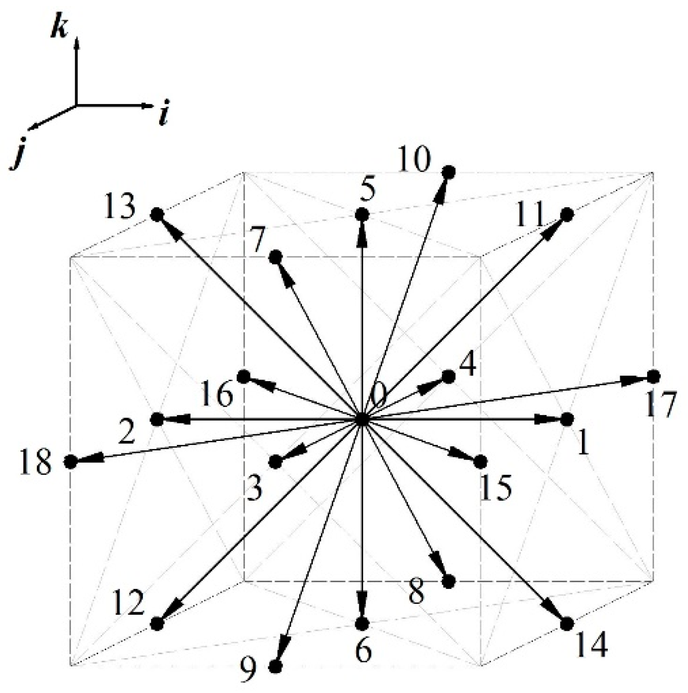
2.1. Lattice Boltzmann Method

The LBM is a relatively new numerical technique for modeling physical system responses. The LBM originated from Lattice Gas Automata. The basic concept of the LBM is to represent fluid as a particle distribution function located at each lattice node. Fluid particles move to neighboring nodes at discrete time steps, colliding with other fluid particles. In the LBM approximation, the fluid is described by a density distribution function f_i(x,t), which describes the particle status at a lattice location x at time t with the discrete velocity e_i. The Boltzmann equation is used to solve the collision-induced evolution of the fluid particle, and the equation can be written as:

$$\frac{\partial f_i}{\partial t}+{\mathit{e}}_i\cdot \nabla f_i\left(x,t\right)={\Omega }_i\left(f_i\right),$$

(1)

where the subscript i represents the directions in which the particle may move. The D3Q19 topology [30] is used in this study, which is a three-dimensional cubic lattice with 19 velocity directions, as illustrated in Figure 1. Ω_i(f_i) is the collision operator; in Nguyen and Ladd’s model [30], Ω_i(f_i) can be written as follows:

$${\mathsf{\Omega }}_i(f_i)={\mathsf{\Omega }}_i(f_i^{eq})+{\displaystyle \sum _j{l}_{ij}{f}_j^{neq}},$$

(2)

where f_j^eq is the local equilibrium function, and f_j^neq is the non-equilibrium function, i.e., $f_j^{neq}=f_j^{}-f_j^{eq}$. The hydrodynamic parameters, such as the mass density ρ and momentum ρu, are the function of the distribution function f and discrete velocity e_i, which can be written as follows:

$$\rho ={\displaystyle \sum _i{f}_i}\hspace{1em}\rho \mathit{u}={\displaystyle \sum _i{f}_i}{\mathit{e}}_i.$$

(3)

The density and momentum should satisfy the mass conservation and momentum conservation. A suitable equilibrium distribution form of the D3Q19 topology can be written as follows [30]:

$$f_i^{eq}=a^{e_i}[\rho +\frac{{\mathit{e}}_i\cdot \rho \mathit{u}}{c_s^2}+\frac{\rho \mathit{u}\mathit{u}:({\mathit{e}}_i{\mathit{e}}_i-c_s^2\mathbf{I})}{2c_s^4}],$$

(4)

where $c_s=\sqrt{c_l^2/3}$ is the speed of sound; $c_l=\Delta x/\Delta t$ is the lattice speed, in which Δx is the lattice space size and Δt is the time step; and |e_i| equals 0 (i = 0), 1(i = 1, 2, …, 6) and $\sqrt{2}$(i = 7, 8, …, 18). The coefficients of the three speeds $a^{e_i}$ are 0 (i = 0), 1/18 (i = 1, 2, …, 6) and 1/36 (i = 7, 8, …, 18).

l_ij are the matrix elements of the linearized collision operator, which must satisfy the following eigenvalue equations:

$${\displaystyle \sum _i{l}_{ij}}=0, {\displaystyle \sum _i{\mathit{e}}_i{l}_{ij}}=0, {\displaystyle \sum _i\overline{{\mathit{e}}_i{\mathit{e}}_i}{l}_{ij}}=\lambda \overline{{\mathit{e}}_j{\mathit{e}}_j}, {\displaystyle \sum _i{e}_i^2{l}_{ij}}={\lambda }_v{e}_j^2,$$

(5)

where $\overline{{\mathit{e}}_i{\mathit{e}}_i}$ is the traceless part of ${\mathit{e}}_i{\mathit{e}}_i$. The first two equations result from the conservation of mass and momentum, and the last two equations describe the isotropic relaxation of the stress tensor. The eigenvalues λ and λ_v are related to the shear viscosity η and bulk viscosity η_v, respectively, which are within the range of −2 < λ < 0, in which $\eta =-\rho c_s^2\left(1/\lambda +1/2\right)$ and ${\eta }_{\nu }=-\rho c_s^2\left[2/(3{\lambda }_{\nu })+1/3\right]$.

A three-parameter collision operator is used in the present study. The post-collision distribution f_i^∗ can be written in the same form as f_i^eq:

$$f_i^{*}=a^{e_i}[\rho +\frac{{\mathit{e}}_i\cdot \rho \mathit{u}}{c_s^2}+\frac{(\rho \mathit{u}\mathit{u}+{\prod }^{neq,*}):({\mathit{e}}_i{\mathit{e}}_i-c_s^2\mathbf{I})}{2c_s^4}],$$

(6)

where ${\prod }^{neq,*}=(1+\lambda ){\displaystyle \overline{{\prod }^{neq}}}+\frac{1}{3}(1+{\lambda }_v)({\prod }^{neq}:\mathbf{I})\mathbf{I}$ and ${\prod }^{neq}=\prod -{\prod }^{eq}$ is the non-equilibrium second moment, in which ${\prod }^{eq}={\displaystyle \sum _i{\mathit{e}}_i}{\mathit{e}}_i{f}_i^{eq}=\rho c_s^2\mathbf{I}+\rho \mathit{u}\mathit{u}$.

Considering an externally imposed force density F, the time evolution of the LBM includes an additional contribution $F_i(x,t)$:

$$f_i(x+{\mathit{e}}_i\Delta t,t+\Delta t)=f_i(x,t)+{\Omega }_i[f(x,t)]+F_i(x,t).$$

(7)

The LBM is well-suited for the specific problem of modeling solid particle suspensions because of its ability to solve particles movement with arbitrary shapes and complex geometries [30,31,32].

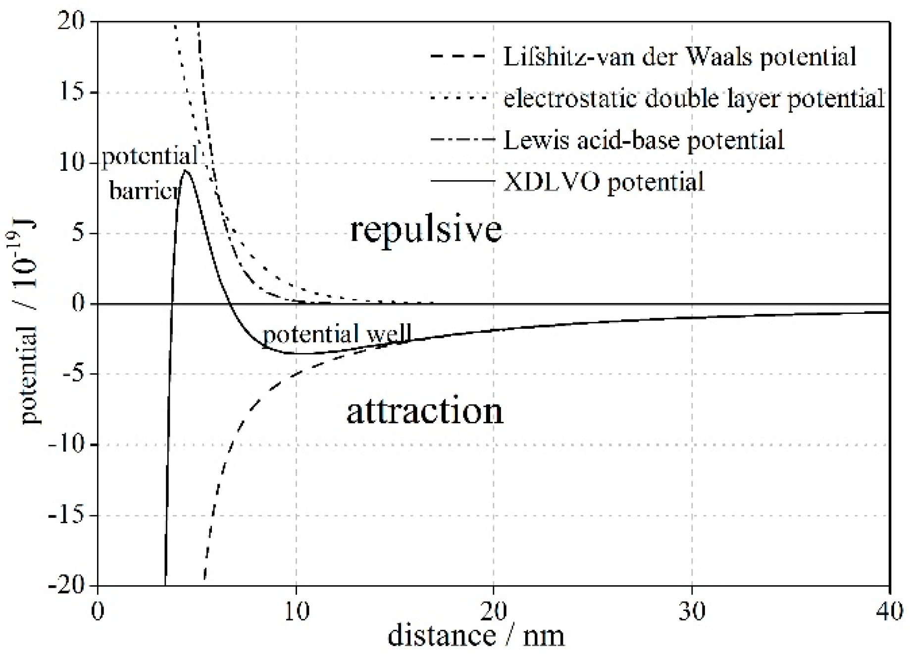
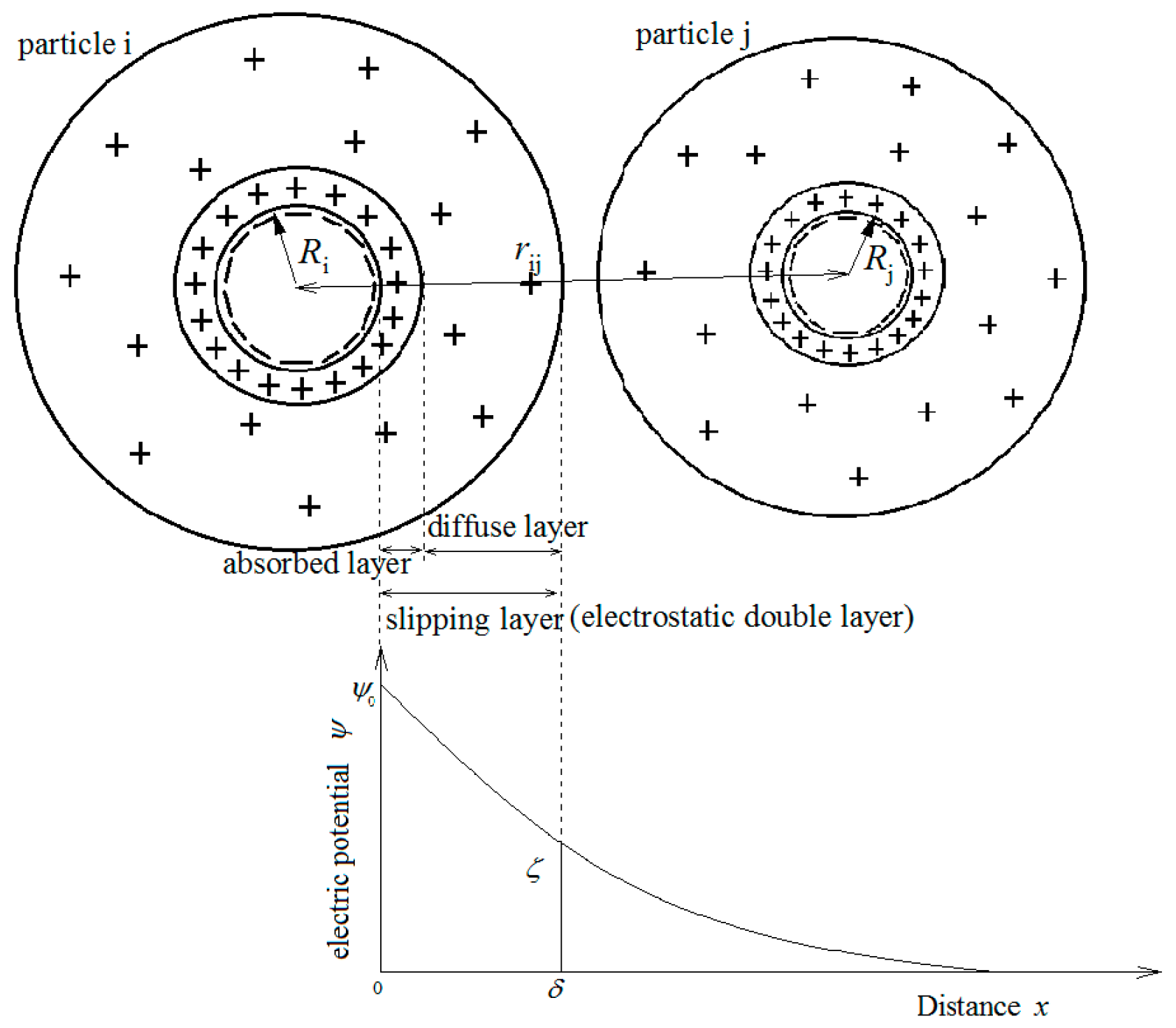
2.2. The Extended Derjaguin–Landau–Verwey–Overbeek Theory

The extended Derjaguin–Landau–Verwey–Overbeek (XDLVO) theory on the interactions of particles can be used to explain the flocculation of cohesive sediment particles [33,34]. According to this theory, there are three short-distance forces acting between particles in aqueous environments (Figure 2), i.e., the Lifshitz‒van der Waals attractive force F^LW_i-j, the electrostatic double-layer repulsive force F^EL_i-j, and the Lewis acid‒base force F^AB_i-j. Each of them is the negative derivative of the corresponding potential to the distance. Among them, temperature only affects the electrostatic double-layer repulsive force by changing the Debye length κ⁻¹. For more details, please refer to [20,26,31,32,33,34,35].

The electrostatic double-layer repulsive force between spherical particles with radii of R₁ and R₂ can be written as follows [20]:

$$F_{\mathrm{EL}i-j}=\frac{4R_1{R}_2}{R_1+R_2}\pi {\epsilon }_0{\epsilon }_r\kappa {\psi }_0{}^2\exp (-\kappa h_{ij}),$$

(8)

where h_ij = r_ij − (R₁ + R₂) is the net distance between spheres, and r_ij is the distance between sphere centers; ε₀ is the dielectric permittivity in a vacuum with a value of 8.854 × 10⁻¹² C²/(J∙m); ε_r is the relative dielectric constant, and for water, it is 78.5; ψ₀ is the surface potential of particles, which is very sensitive to salinity and pH but not sensitive to temperature when the temperature is below approximately 150 °C [36]; κ⁻¹ is the Debye length, related to temperature, cation valence, and ion concentration, which can be written as follows:

$$\kappa ={(2e_0^2{N}_{\mathrm{A}}cz/({\epsilon }_0{\epsilon }_{r}kT))}^{1/2},$$

(9)

where $e_0$ is the element charge 1.6 × 10⁻¹⁹ C; $N_{\mathrm{A}}$ is Avogadro’s number 6.022 × 10²³/mol; k is the Boltzmann constant 1.38 × 10⁻²³ J/K; T is the absolute temperature with a unit of K; c is the cation concentration with a unit of mol/L; and z represents the cation valence and is dimensionless.

2.3. Criterion Distance of Flocculation

Yang et al. [37] mentioned that the aggregation sign of cohesive sediment should be the contact of the sliding surface. They suggested that the anions are distributed on the surface of particles, and adsorb the cations in the media. The zone with cations can be separated into two layers, the inner layer with a high density of cations, which is called the absorbed layer, and the outer layer with less cations, which is called the diffuse layer, as illustrated in Figure 3. Yang et al. [37] consider that when the surface distance is less than twice the thickness of the slipping layer, the particles are wrapped by a common slipping layer, and they form a new or enlarge an old floc. The electric potential decays exponentially at large distance with decay length given by the Debye length κ⁻¹, with ψ₀ on the particle surface and ζ at the distance δ. Both ψ₀ and ζ can be measured in experiments, thus the slipping layer thickness δ can be calculated as follows:

$$\delta =\frac{1}{\kappa }\ln \frac{1+exp\left(ze\psi T/2k\right)}{1-exp\left(ze\psi T/2k\right)},$$

(10)

where δ is the slipping layer thickness when the potential ψ equals the zeta-potential ζ. From Equations (9) and (10), a rising temperature will thicken δ. Thus, twice the value of δ was taken as the criterion distance for flocculation.

3. Computational Conditions

Four cases were set up to study the influence of temperature on the bulk settlement of cohesive sediment. The temperatures were 5 °C, 10 °C, 20 °C, and 30 °C in the four cases. The domain calculation area was 0.288 mm × 6 mm × 0.240 mm, and the space precision was 2 μm, thus a total of 144 lu × 3000 lu × 120 lu (lattice unit). The surroundings were defined as periodic boundaries, and the upper and lower boundaries were set as solid no-slip boundaries. The initial sediment concentration was set to 1.3 kg/m³ (volume concentration of 0.049%). Eight hundred sediment particles with diameters from 5 μm to 10 μm were scatted randomly in the whole calculation area. The calculation time step was set as 10⁻⁶ s, and the total time was 20 s. In all cases, the cation was selected as Na⁺, with a valence of +1 and a concentration of 0.085 mol/L or salinity of 5 ppt. Illite was considered to be the clay mineral with a surface potential of −27.22 mV [38] as illite is widely distributed and its chemical and physical properties that needed in this study are easy to obtain as they are studied more extensively. The sediment density was ρ_s = 2650 kg/m³. The water density was ρ = 1000 kg/m³, without considering the influence of salinity and temperature as the error of the density at the values adopted will be less than 4% according to the sea water state equation proposed by UNESCO [39]. The other parameters are listed in

Table 1. Parameters in each case.

Case ID	#1	#2	#3	#4
Temperature/(°C)	5	10	20	30
2δ/(nm)	18.7	19.1	20.0	20.7
Water viscosity ν/(10−6 m2 s−1)	1.52	1.31	1.00	0.80

.

4. Results

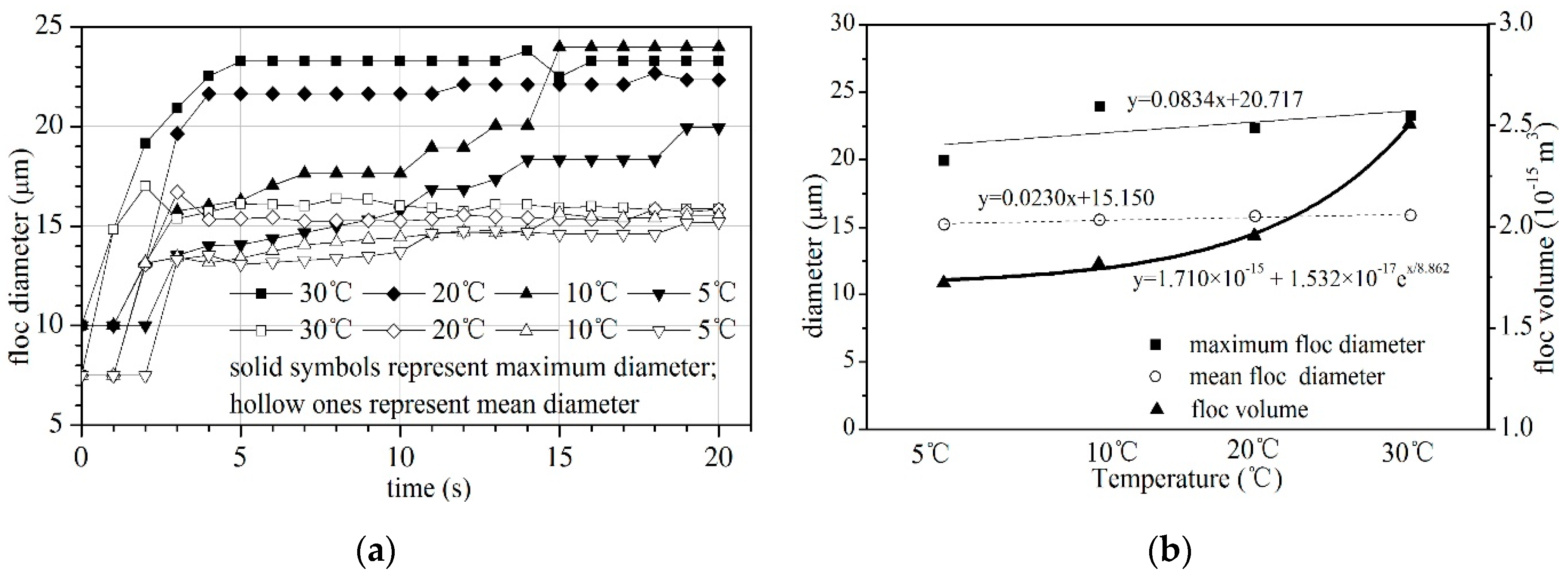
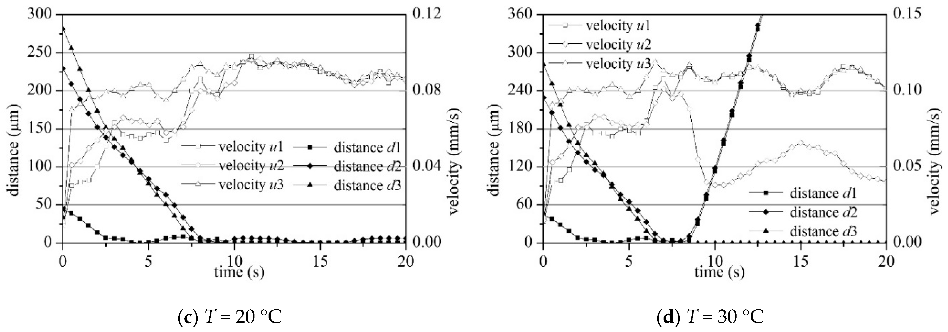
4.1. Floc Size and Floc Volume

Floc size and volume are two of the floc properties that are easy to obtain from the numerical results. Figure 4a shows the time series of the maximum and mean floc sizes. The final results of them and the floc volume are shown in Figure 4b. Floc volume is a sum of the volumes of all the flocs, and indicates the content of floc in the suspended column. During the same settling period, both the floc sizes and floc volume increased with increasing temperature.

At the end of the simulation, in the cases of 5 °C, 10 °C, 20 °C, and 30 °C, the maximum floc sizes were 20.0 μm, 24.0 μm, 22.3 μm, and 23.3 μm, respectively, with the peak value at 10 °C. In the cases of 20 °C and 30 °C, the maximum floc sizes fluctuated slightly in the latter phase (Figure 4a).

The mean floc size increased slightly but more stably than the maximum size did, from 15.2 μm at 5 °C to 15.5 μm at 10 °C, 15.8 μm at 20 °C, and 15.9 μm at 30 °C. The floc volume increased more obviously than the floc size. They were 3.8% at 5 °C, 4.0% at 10 °C, 4.3% at 20 °C, and 5.5% at 30 °C (Figure 4b).

4.2. Settling and Flocculation Process

The microscopic process of settling and flocculation might explain the preceding phenomenon. This process can be easily given out via the numerical simulations. Three particles numbered #681, #689, and #721 were selected to illustrate the settling process. In all four cases, they had formed or almost formed a floc.

The corresponding diameters for particles #681, #689, and #721 were 6.00 μm, 7.16 μm, and 9.36 μm, respectively. The distance between the primary particles and their velocities at different temperatures are plotted in Figure 5.

At the beginning, the large particle falling fast was on top of the small one with a low speed, resulting in a diminishing net distance between them before they met, as is common in all cases. At a low temperature (5 °C, Figure 5a), the three primary particles cannot get close enough to form a new floc, and fell individually. The velocities of the particles increased when they collided (12.5 s to 17.5 s), but finally they readjusted to their initial speed with the increasing distance between each other. At a medium temperature (10 °C and 20 °C, Figure 5a,b), the three particles formed a floc and settled together with a common speed higher than that of each primary particle; however, the time when the floc formed was earlier at 20 °C than that at 10 °C. In the case of high temperature (30 °C, Figure 5d), the small particle (#681) was first captured by the medium one (#689), forming an unstable floc, which was destroyed by the collision of the large particle (#721), and then flocculated with the large particle, leaving the medium particle settling individually with a low speed.

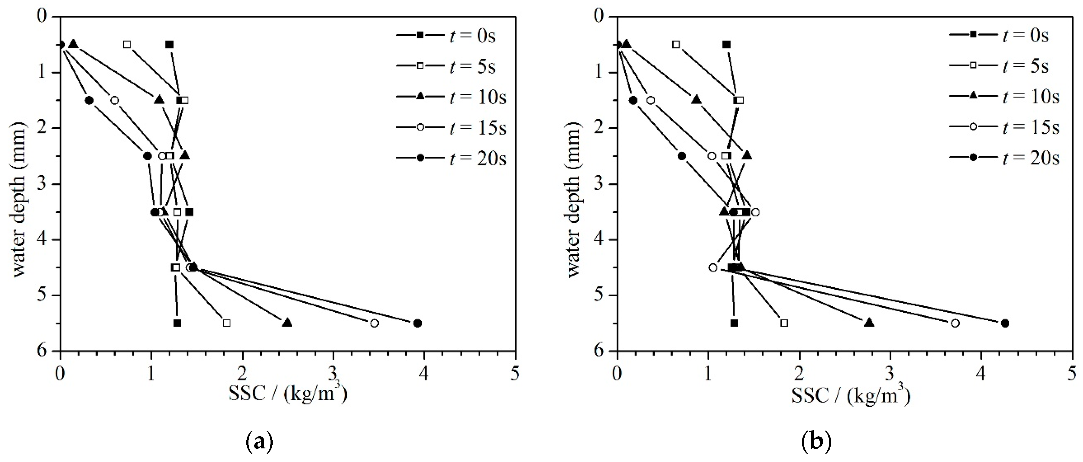
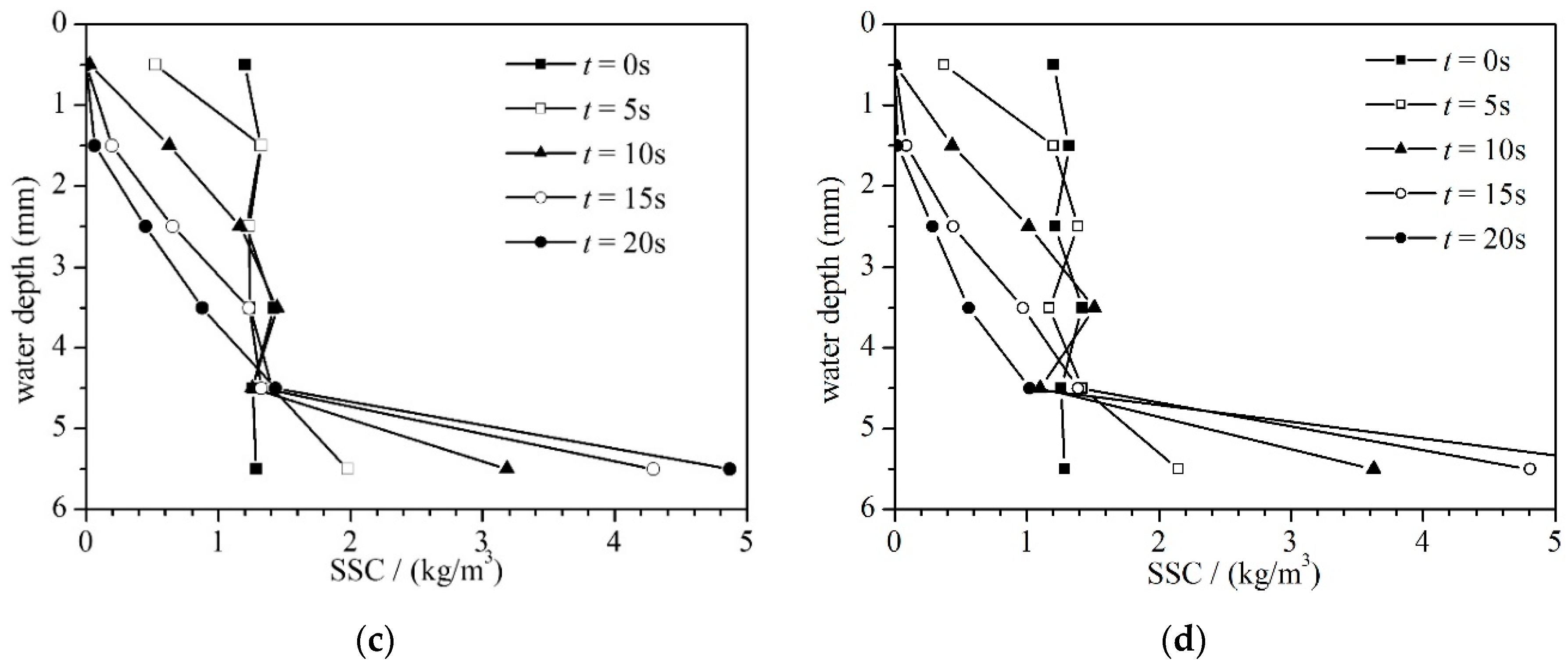
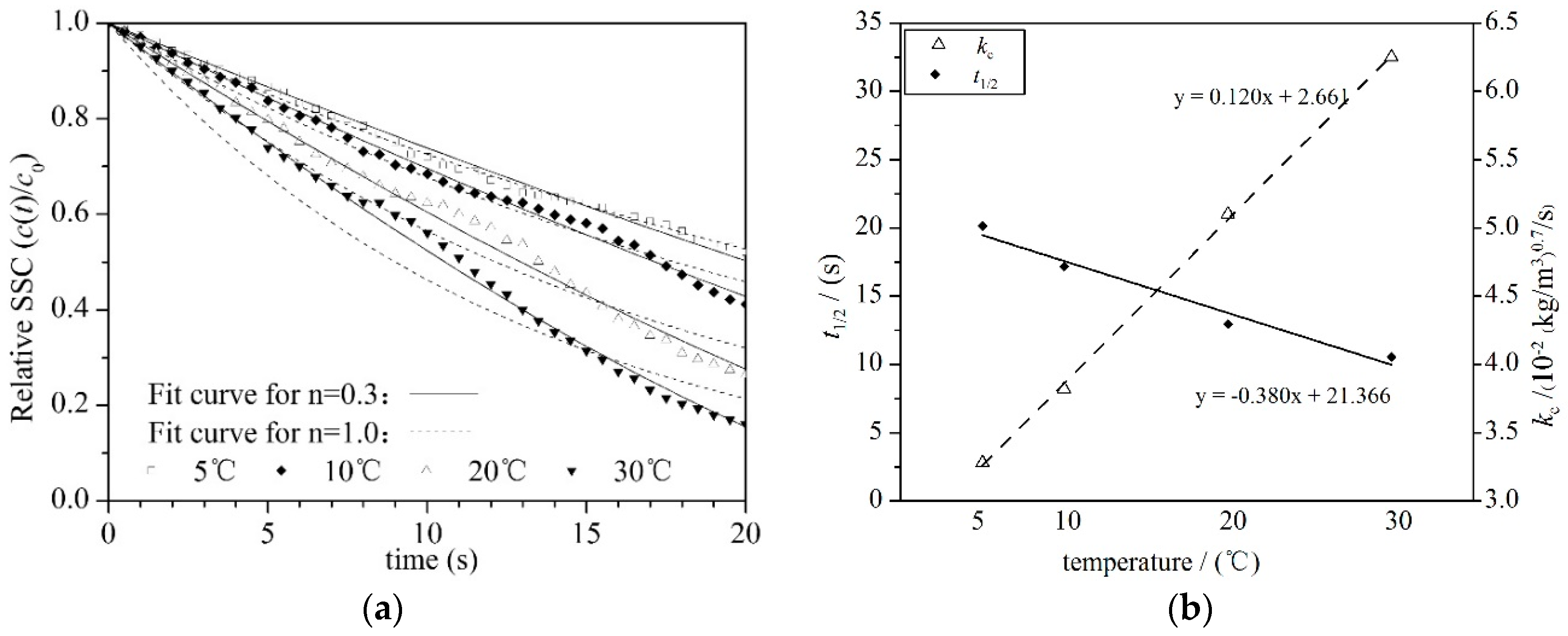
4.3. Suspended Sediment Concentration

Figure 6 illustrates the variation in SSC for each case every 5 s. It is shown that, in all four cases, SSCs above 4.0 mm continued to decline, while those at the bottom layers were increasing. They remained relatively stable in the 4.0–5.0 mm layer, but a small difference can be seen between the cases: the SSC in this layer went up slightly in the 5 °C case, but had a slight reduction in the 30 °C case, and stayed nearly constant in the other two cases.

Chen and Shao [40] revealed that the SSC change rate in still water was generally fitted to a first-order equation as follows:

$$\frac{\mathrm{d}C}{\mathrm{d}t}=-k_{c}C.$$

(11)

where k_c is the attenuation coefficient, in which a large value indicates a faster incline.

The time series curves of relative SSC (ratio of c(t) at time t to initial c₀) of water depths shallower than 4.5 mm, in which layer the SSC is somewhat unchanged as shown in Figure 6, are draw in Figure 7a. As shown in Figure 7a, the fitting results of Equation (11) (the dash lines) were less superior in these cases, therefore, some trials of indexes of n for C in the right side had been done. As a result, 0.3 was the best fitted index (the solid lines in Figure 7a), thus yielding the following formula:

$$\frac{\mathrm{d}C}{\mathrm{d}t}=-k_c{C}^{0.3}.$$

(12)

The time when the SSC reduced to half of the initial SSC was taken as the half-life settlement period t_1/2. From Equation (12), the half-life period t_1/2 can be written as follows:

$$t_{1/2}=-\frac{c_0^{0.7}}{0.7k_c}\left({\left(1/2\right)}^{0.7}-1\right).$$

(13)

The k_c and half-life period t_1/2 can be solved from the fitting curve in Figure 7a and they are shown in Figure 7b. The temperature increase had a positive effect on k_c and a negative effect on t_1/2, indicating a faster change in SSC at high temperatures than at low temperatures.

4.4. Sediment Settling Velocity

In numerical simulations, the bulk velocities can be statistically analyzed from microscope by averaging the velocities of individual particles and flocs, which are the directional output of the simulation, with a weight of each volume; however, they are commonly difficult to measure directly in physical experiments. As a result, the bulk velocity is often calculated from the SSC half-life period t_1/2 and the settling distance [6]. The bulk velocity can be expressed simply as follows:

$$\overline{u(h)}=H/\left(2t_{1/2}\right),$$

(14)

where $\overline{u(H)}$ is the time-averaged (from 0 to t_1/2) bulk settling velocity at water depth H, in which depth the SSC changes slightly during settling, and that is why 4.5 mm (4.0–5.0 mm) is chosen in Figure 7a. The derivation of Equation (14) can refer to You’s work [41]. The water depth H and time t_1/2 in Equation (14) can be obtained easily through macroscopic observation.

In

Table 2. Bulk settling velocity of different methods (velocity 1 v₁ is derived from H and t_1/2; velocity 2 v₂ is the statistical result of all particles and flocs at water depths from 4.0 mm to 5.0 mm; ABS(1-2) |v₁−v₂| means the absolute difference between velocity 1 and velocity 2; |v₁−v₂|/(|v₁+v₂|/2) represents the relative difference between velocity 1 and velocity 2).

Temperature/(°C)	5	10	20	30
(1) velocity 1 v1/(mm/s)	0.099	0.117	0.155	0.189
(2) velocity 2 v2/(mm/s)	0.101	0.117	0.152	0.185
(3) ABS(1-2) |v1−v2|/(mm/s)	0.002	0.000	0.003	0.004
(4) |v1−v2|/(|v1+v2|/2)/(%)	2.0%	0.0%	2.0%	2.1%

, velocity 1 summarized the bulk velocity calculated from Equation (14) with the parameters in Figure 7b. The time-averaged statistical velocities during the period of 0–t_1/2 in the 4.5 mm layer (4.0–5.0 mm) were listed in Table 2, as velocity 2. The results of the two methods were almost identical, with a small relative error of approximately 2%. Equation (14) can be taken as the connection between the microscopic statistical methods and physical test methods.

The floc velocities are also compared with the data of Xia et al. [12], Khelifa and Hill [16], Guo and He [13], Dyer and Manning [42], and Manning et al. [43] and the formulas of Manning et al. [43], Khelifa and Hill [16] and Winterwerp [44] in Figure 8a. The primary particle diameter in the simulations ranged from 5 μm to 10 μm, and the simulated floc settling velocities lie between Winterwerp’s [44] lines with primary particle sizes of 1 μm and 20 μm, and most of them between Khelifa and Hill’s [13] lines with the same primary sizes. They also are between Manning et al.’s [43] lines with an effective density of 160 kg/m³ and 1600 kg/m³, but closer to the line of 1600 kg/m³, probably due to the small size of the flocs, so they have a larger effective density [16,42]. The simulation results overlap with the in situ observation data of Xia et al. [12] for July 1999 and January 2000. It should be noted that the simulation velocities are each floc’s speed, while that of other studies are bulk velocity, or statistical macro data of suspended samples.

Figure 8b illustrates the variation of average floc velocities in different temperature conditions, including the observational data from Xia et al. [12] and Guo and He [43], the experimental data from Wan et al. [6], and the simulation results of LBM. The settling speed differs greatly owing to factors other than temperature, such as SSC, labeled in the legend; however, all the studies reveal a trend of the settling velocity increasing with the water temperature. The velocity change rate with temperature of this numerical result is 0.0382 mm/s/°C—larger than the rate of Wan et al.’s [6] physical experiment results of low SSC (0.0248 mm/s/°C), smaller than that of Wan et al.’s [6] high SSC (0.0513 mm/s/°C) and Xia et al.’s [12] observation results (0.1031 mm/s/°C), and very close to Guo and He’s [43] observation data (0.0364 mm/s/°C).

5. Discussion

The above results indicate that the LBM is reasonable for using in modeling bulk settling velocity and that some collisions led to aggregation, while others did not, or, on the contrary, to disaggregation. On referring to Kim and Stolzenbach’s work [45], the ratio of the global collision number to the total particle number is defined as the collision frequency η_glo, the ratio of collisions that created new flocs or enlarged original flocs to the total collisions is the capture frequency η_cap, and the product of the two ratios is the aggregation frequency E_agg = η_glo × η_cap. The three parameters were analyzed and are illustrated in Figure 9.

As shown in Figure 9a, with increasing temperature, η_glo continued to grow up, while η_cap began to decline slightly after its peak at about 20 °C after an initial increase. Sterling et al. [46] stated that the collision frequency was due to three factors: Brownian motion, turbulence shear, and differential settling. In this simulation, the sediment particles were much larger than the molecule and thus the Brownian motion could be ignored; the turbulence effect was omissible in still water; therefore, the main factor was the differential settling. Figure 9b showed a positive correlation between η_glo and settling velocity, which was consistent with the viewpoint of Sterling et al. [46]. η_glo in the simulations ranges from 2.1% to 4.2%, very close to the results of Kim and Stolzenbach [45] (from 2.96% to 3.20%). The potential reasons for the difference between the two results might lie in Kim and Stolzenbach’s [45] presumption that their model neglected the repulsive colloidal interaction, which is very sensitive to temperature (in Section 2.2) but was not mentioned in their study, so they might not take the temperature into account in their work.

When the distance between two particles was less than 25 nm, the three short-distance forces were the most important. Among the forces, only the electrostatic double-layer repulsion force is related to the temperature. From Figure 10a, the repulsive force was higher at a high temperature or a short distance between two particles. Additionally, the rising temperature thickened the slipping layer (Table 1). Taken together, at a distance of twice the slipping layer thickness (the distance value of the left point of each curve in Figure 10), the particles must overcome a stronger repulsion force before flocculation at high temperature than at low temperature. Thus, the higher the temperature, the greater the capture frequency, as noted by Qiao et al.’s simulation of two primary particles [26].

However, the situation was different when considering multiple particles. Also, taking the above three particles in the 30 °C case as an example, when the large particle (#721) met the floc formed by the other two particles, this particle seized the small one (#681) and a new floc was formed, with particle #689 settling individually. This collision produced a new floc, but disaggregated an old floc, giving no change in the number of flocs and particles; thus, η_cap remained unchanged, while in the 20 °C case this collision made the η_cap larger as it enlarged the floc. From the aspect of force, when a third particle was involved, the difference between the two double-layer forces acting on particle #681, F_EL681–689–F_EL681–721, was the same in magnitude as the particle gravity (Figure 10b), and the macroscopic force, including the gravity and hydrodynamic force, was highlighted. The higher the temperature, the more obvious the macro forces were.

This phenomenon reveals that, at high temperature, few large flocs broke into small ones because of collision, resulting in a fluctuation of time series and a decrease in the maximum floc size, as illustrated in Figure 4a. However, the mean floc size and total floc volume did not decrease (in Figure 4b) because the large flocs that were collapsed by collision had a very small proportion and were only decreased in size but rarely dispersed into primary particles.

A detailed force analysis of a large floc is more convincing but more complex when it is comprised of more primary particles because of its continuous changing spatial statuses and complicated interactive forces. Although the analysis of the floc of three primary particles is limited, it illustrates the flocculation formation and breakage at different temperatures. From the analysis, it is certain that, at high temperature, the macroscopic force becomes more obvious due to the small difference of short-distance forces between particles. The above analysis qualitatively explains why the fracture frequency increases at high temperatures, which is the main cause of the decrease in η_cap. However, the reason is different for the low-temperature case, where the large repulsion force makes it more difficult for the particles to get close enough to form flocs, resulting in a small η_cap.

The above results could be explained by the present LBM model, but there is still an obvious shortage in that the flocs in each case were not sufficient in quantity and size. This shortage is because the LBM requires a large number of grids to describe the solid‒fluid boundary and micro properties of each sediment particle; thus, the computational cost of the LBM is extremely high. Each case in this study took three months on a supercomputer with 288 CPUs. A higher computational cost is expected if the sediment bulk properties are described in more detail. That is the reason for the less convincing results of the present study. Therefore, subsequent studies will involve further optimizing the calculation method and case design for better simulation results. In a natural environment, changes in other factors, such as water salinity, turbulence, and SSC, are unavoidable, so their influences on flocculation will be further studied by LBM in the future.

6. Conclusions

The bulk settling and flocculation process of cohesive sediment containing primary particles of sizes of 510.0 μm in still water at various temperatures was simulated via the LBM. The floc size and volume were analyzed, and the effect of temperature on bulk settling was studied based on the macroscopic SSC change and microscopic statistics of particle and floc settling velocity. The difference of the properties at different temperatures was explained by the formation of flocs, aggregation frequency, and forces between particles. The following conclusions were obtained:

(1)

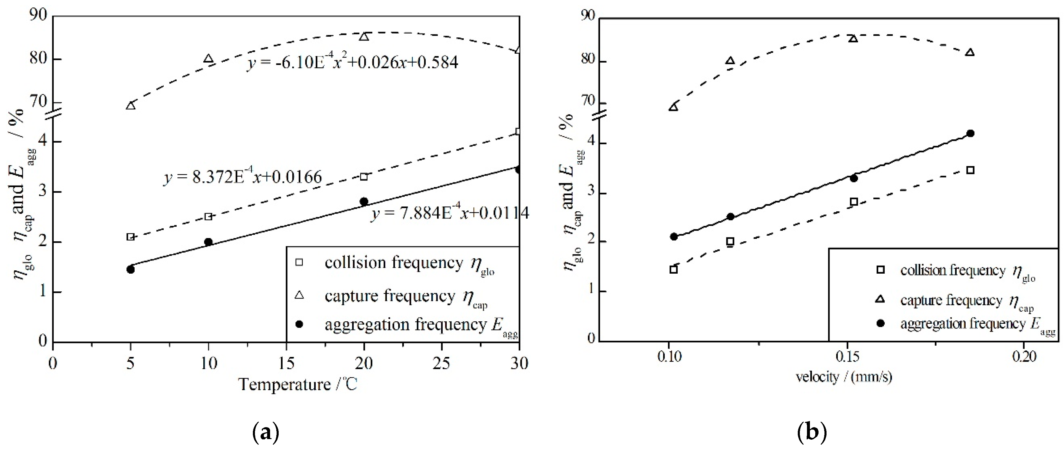
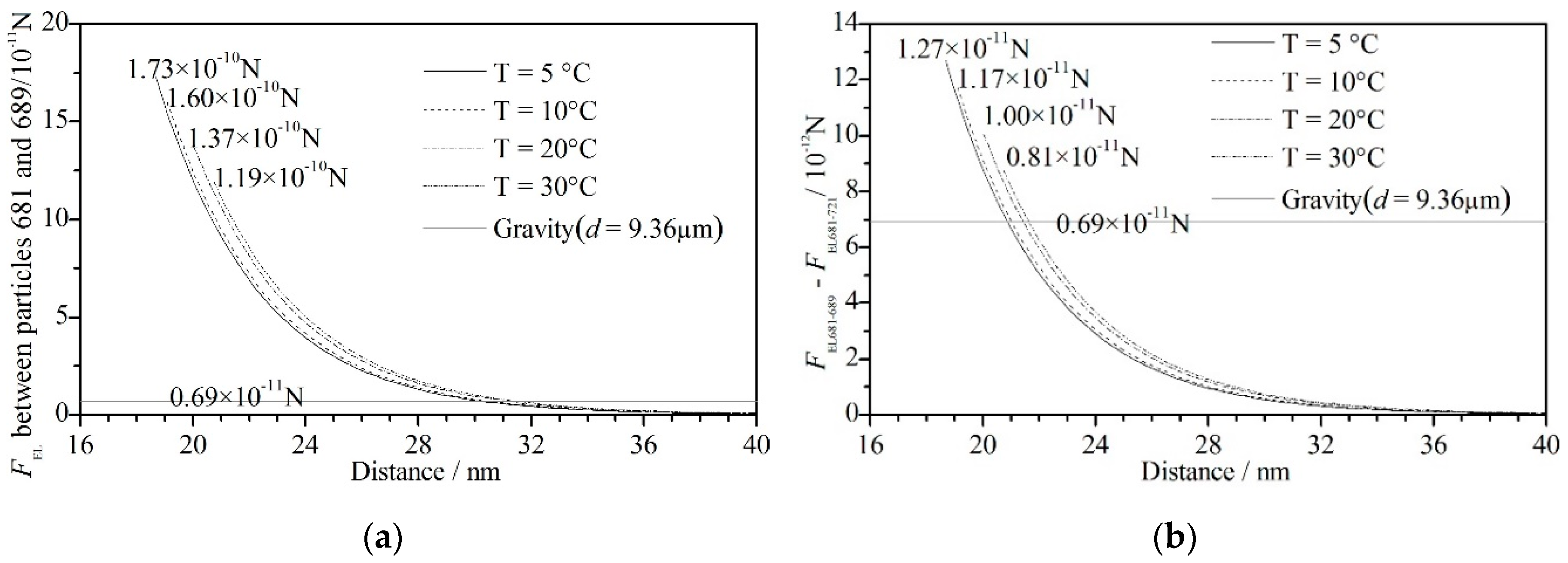
The mean floc size and floc volume increased with increasing temperature. The maximum floc size initially increased and then decreased slightly with its peak at 10 °C and trough at 5 °C. The floc was not easily formed at low temperature but was unstable and cracked easily at high temperature. The aggregation process, aggregation frequency and forces between particles can be explained by the above. At low temperatures, the collision frequency η_glo and capture frequency η_cap were low, which meant the floc was not easily formed; at high temperatures, the large flocs were easily broken as the weighting of the macro force increased to have the same magnitude as the short-distance force.

(2)

During settling, the SSC time series curves fit well with the equation $\mathrm{d}C/\mathrm{d}t=-k_c{C}^{0.3}$, from which the settlement half-life period and bulk setting velocity were deduced. Increasing the temperature had a negative effect on the settlement half-life, indicating a faster SSC incline at high temperatures than at low temperatures.

(3)

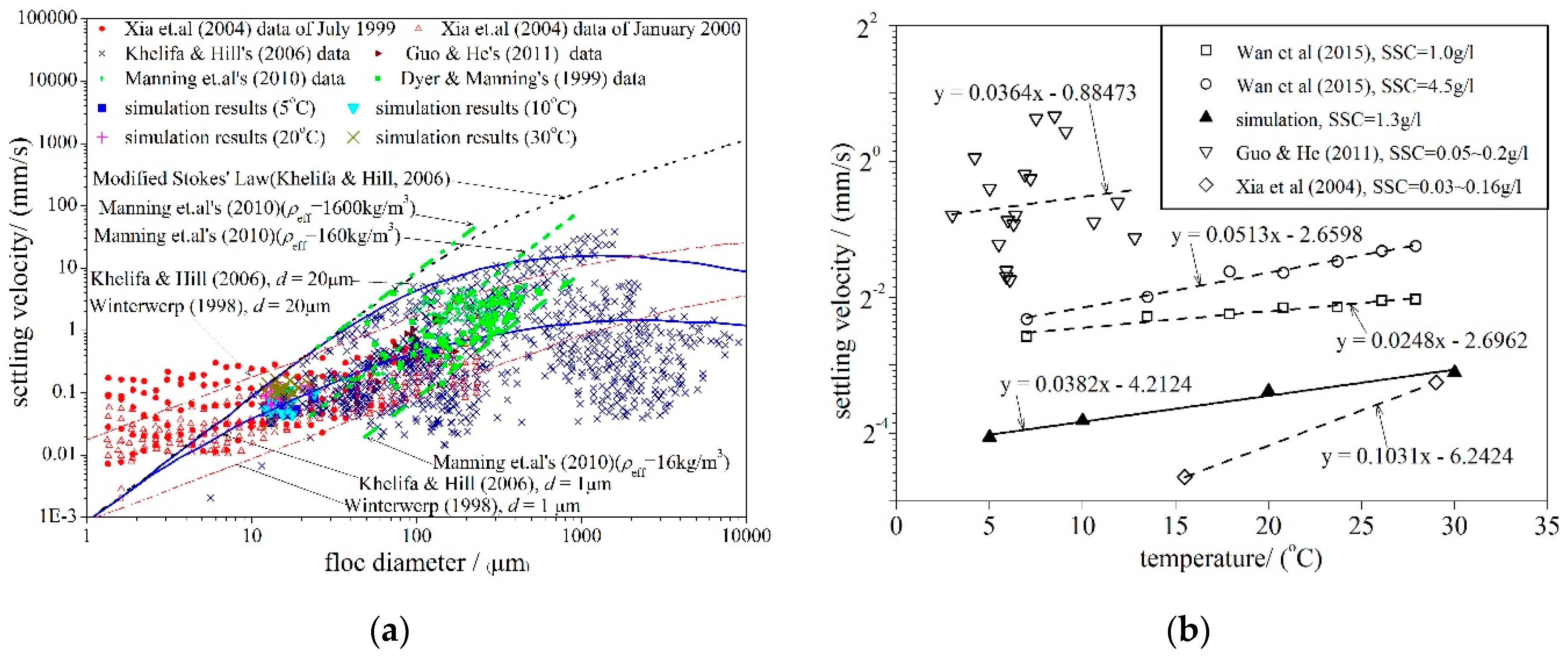
The macroscopic bulk velocity derived from the SSC change agreed well with the microscopic statistical settling velocity of each particle and floc. Both velocities agreed well with the existing physical test results, on-site observation data, and formulas, indicating that the LBM is a reasonable choice for simulating cohesive sediment bulk settling.

References

1. Winterwerp, J.C. On the flocculation and settling velocity of estuarine mud. Cont. Shelf Res. 2002, 22, 1339–1360. [Google Scholar] [CrossRef]
2. Mietta, F.; Chassagne, C.; Manning, A.J.; Winterwerp, J.C. Influence of shear rate, organic matter content, ph and salinity on mud flocculation. Ocean Dyn. 2009, 59, 751–763. [Google Scholar] [CrossRef]
3. Ha, H.K.; Maa, J.P.Y. Effects of suspended sediment concentration and turbulence on settling velocity of cohesive sediment. Geosci. J. 2010, 14, 163–171. [Google Scholar] [CrossRef]
4. Jiang, G.; Zhou, H.; Ruan, W.; Yao, S.; Zhang, Z.; Zhao, L. Influence of water temperature on mud particle deposition—Laboratory tests. J. Coast. Res. 2004, 20, 59–66. [Google Scholar]
5. Etemad-shahidi, A.; Shahkolahi, A.; Liu, W.C. Modeling of hydrodynamics and cohesive sediment processes in an estuarine system: Study case in Danshui river. Environ. Model. Assess. 2010, 15, 261–271. [Google Scholar] [CrossRef]
6. Wan, Y.; Wu, H.; Roelvink, D.; Gu, F. Experimental study on fall velocity of fine sediment in the Yangtze Estuary, China. Ocean Eng. 2015, 103, 180–187. [Google Scholar] [CrossRef]
7. Dickhudt, P.J.; Friedrichs, C.T.; Schaffner, L.C.; Sanford, L.P. Spatial and temporal variation in cohesive sediment erodibility in the York River estuary, eastern USA: A biologically influenced equilibrium modified by seasonal deposition. Mar. Geol. 2009, 267, 128–140. [Google Scholar] [CrossRef]
8. Lau, Y.L. Temperature effect on settling velocity and deposition of cohesive sediments. J. Hydraul. Res. 1994, 32, 41–51. [Google Scholar] [CrossRef]
9. Owen, M.W. The Effect of Temperature on the Settling Velocities of an Estuary Mud; Hydraulics Research Station Report, No. INT 106; Hydraulics Research Station: Wallingford, UK, 1972. [Google Scholar]
10. Lee, B.J.; Fettweis, M.; Toorman, E.; Molz, F.J. Multimodality of a particle size distribution of cohesive suspended particulate matters in a coastal zone. J. Geophys. Res. Oceans. 2012, 117, C03014. [Google Scholar] [CrossRef]
11. Andersen, T.J.; Pejrup, M. Biological mediation of the settling velocity of bed material eroded from an intertidal mudflat, the Danish Wadden Sea. Estuar. Coast. Shelf Sci. 2002, 54, 737–745. [Google Scholar] [CrossRef]
12. Xia, X.M.; Li, Y.; Yang, H.; Wu, C.Y.; Sing, T.H.; Pong, H.K. Observations on the size and settling velocity distributions of suspended sediment in the Pearl River Estuary, China. Cont. Shelf Res. 2004, 24, 1809–1826. [Google Scholar] [CrossRef]
13. Guo, L.; He, Q. Freshwater flocculation of suspended sediments in the Yangtze River, china. Ocean Dyn. 2011, 61, 371–386. [Google Scholar] [CrossRef]
14. Winterwerp, J.C.; Van Kesteren, W.G.M. Introduction to the Physics of Cohesive Sediment in the Marine Environment; Elsevier: Amsterdam, The Netherlands, 2004; ISBN 0-444-51553-4. [Google Scholar]
15. Grabowski, R.C.; Droppo, I.G.; Wharton, G. Erodibility of cohesive sediment: The importance of sediment properties. Earth Sci. Rev. 2011, 105, 101–120. [Google Scholar] [CrossRef]
16. Khelifa, A.; Hill, P.S. Models for effective density and settling velocity of flocs. J. Hydraul. Res. 2006, 44, 390–401. [Google Scholar] [CrossRef]
17. Manning, A.J.; Dyer, K.R. Mass settling flux of fine sediments in Northern European estuaries: Measurements and predictions. Mar. Geol. 2007, 245, 107–122. [Google Scholar] [CrossRef]
18. Baugh, J.V.; Manning, A.J. An assessment of a new settling velocity parameterisation for cohesive sediment transport modeling. Cont. Shelf Res. 2007, 27, 1835–1855. [Google Scholar] [CrossRef]
19. Markussen, T.N.; Andersen, T.J. A simple method for calculating in situ floc settling velocities based on effective density functions. Mar. Geol. 2013, 344, 10–18. [Google Scholar] [CrossRef]
20. Zhang, J.; Zhang, Q. Hydrodynamics of fractal flocs during settling. J. Hydrodyn. Ser. B 2009, 21, 347–351. [Google Scholar] [CrossRef]
21. Tang, S.; Preece, J.M.; McFarlane, C.M.; Zhang, Z. Fractal morphology and breakage of DLCA and RLCA aggregates. J. Colloid Interface Sci. 2000, 221, 114–123. [Google Scholar] [CrossRef]
22. Weber-Shirk, M.L.; Lion, L.W. Flocculation model and collision potential for reactors with flows characterized by high Peclet numbers. Water Res. 2010, 44, 5180–5187. [Google Scholar] [CrossRef] [PubMed]
23. Maerz, J.; Verney, R.; Kai, W.; Feudel, U. Modeling flocculation processes: Intercomparison of a size class-based model and a distribution-based model. Cont. Shelf Res. 2011, 31, S84–S93. [Google Scholar] [CrossRef]
24. Yang, Z.; Yang, H.; Jiang, Z.; Huang, X.; Li, H.; Li, A.; Cheng, R. A new method for calculation of flocculation kinetics combining Smoluchowski model with fractal theory. Colloids Surf. A Physicochem. Eng. Asp. 2013, 423, 11–19. [Google Scholar] [CrossRef]
25. Zhang, J.F.; Maa, P.Y.; Zhang, Q.H.; Shen, X.T. Direct numerical simulations of collision efficiency of cohesive sediments. Estuar. Coast. Shelf Sci. 2016, 178, 92–100. [Google Scholar] [CrossRef]
26. Qiao, G.Q.; Zhang, J.F.; Zhang, Q.H. Study on the influence of temperature to cohesive sediment flocculation. J. Sediment Res. 2017, 42, 35–40. (In Chinese) [Google Scholar]
27. Ladd, A.J.C. Numerical simulations of particulate suspensions via a discretized Boltzmann equation. Part 1. Theoretical foundation. J. Fluid Mech. 1994, 271, 285–310. [Google Scholar] [CrossRef]
28. Ladd, A.J.C. Numerical simulations of particulate suspensions via a discretized Boltzmann equation. Part 2. Numerical results. J. Fluid Mech. 1994, 271, 311–339. [Google Scholar] [CrossRef]
29. Ladd, A.J.C.; Verberg, R. Lattice-Boltzmann simulations of particle-fluid suspensions. J. Stat. Phys. 2001, 104, 1191–1251. [Google Scholar] [CrossRef]
30. Nguyen, N.Q.; Ladd, A.J. Lubrication corrections for Lattice-Boltzmann simulations of particle suspensions. Phys. Rev. E. 2002, 66, 046708. [Google Scholar] [CrossRef]
31. Zhang, J.F.; Zhang, Q.H. Lattice Boltzmann simulation of the flocculation process of cohesive sediment due to differential settling. Cont. Shelf Res. 2009, 31, S94–S105. [Google Scholar] [CrossRef]
32. Zhang, J.F.; Zhang, Q.H.; Qiao, G.Q. A lattice Boltzmann model for the non-equilibrium flocculation of cohesive sediments in turbulent flow. Comput. Math. Appl. 2014, 67, 381–392. [Google Scholar]
33. Van Oss, C.J. Interfacial Forces in Aqueous Media; CRC Press: Boca Raton, FL, USA, 1994; ISBN 978-1420015768. [Google Scholar]
34. Hoek, E.M.V.; Agarwal, G.K. Extended DLVO interactions between spherical particles and rough surfaces. J. Colloid Interface Sci. 2006, 298, 50–58. [Google Scholar] [CrossRef] [PubMed]
35. Qiao, G.Q.; Zhang, Q.H.; Zhang, J.F.; Cheng, H.J.; Lu, Z. Lattice Boltzmann model of cohesive sediment flocculation simulation based on the XDLVO theory. J. Tianjin Univ. 2013, 46, 232–238. (In Chinese) [Google Scholar]
36. Vinogradov, J.; Jackson, M.D. Zeta potential in intact natural sandstones at elevated temperatures. Geophys. Res. Lett. 2015, 42, 6287–6294. [Google Scholar] [CrossRef]
37. Yang, T.S.; Xiong, X.Z.; Zhan, X.L.; Yang, M.Q. The study on slipping water layers of cohesive sediment particles. J. Hydraul. Eng. 2002, 33, 20–26. (In Chinese) [Google Scholar]
38. Sondi, I.; Bišćan, J.; Pravdić, V. Electrokinetics of pure clay minerals revisited. J. Colloid Interface Sci. 1996, 178, 514–522. [Google Scholar] [CrossRef]
39. Tenth Report of the Joint Panel on Oceanographic Tables and Standards, Sidney, B.C. Canada, 1–5 September 1980; UNESCO Technical Papers in Marine Science No. 36; UNESCO: Paris, France, 1981.
40. Chen, H.S.; Shao, M.A. Effect of NaCl concentration on dynamic model of fine sediment flocculation and settling in still water. J. Hydraul. Eng. 2002, 8, 63–67. (In Chinese) [Google Scholar]
41. You, Z.J. The effect of suspended sediment concentration on the settling velocity of cohesive sediment in quiescent water. Ocean Eng. 2004, 31, 1955–1965. [Google Scholar] [CrossRef]
42. Dyer, K.R.; Manning, A.J. Observation of the size, settling velocity and effective density of flocs, and their fractal dimensions. J. Sea. Res. 1999, 41, 87–95. [Google Scholar] [CrossRef]
43. Manning, A.J.; Langston, W.J.; Jonas, P.J.C. A review of sediment dynamics in the Severn Estuary: Influence of flocculation. Mar. Pollut. Bull. 2010, 61, 37–51. [Google Scholar] [CrossRef]
44. Winterwerp, J.C. A Simple Model for Turbulence Induced Flocculation of Cohesive Sediment. J. Hydraul. Res. 1998, 36, 309–326. [Google Scholar] [CrossRef]
45. Kim, A.S.; Stolzenbach, K.D. Aggregate formation and collision efficiency in differential settling. J. Colloid Interface Sci. 2004, 271, 110–119. [Google Scholar] [CrossRef] [PubMed]
46. Sterling, M.C., Jr.; Bonner, J.S.; Ernest, A.N.S.; Page, C.A.; Autenrieth, R.L. Application of fractal flocculation and vertical transport model to aquatic sol-sediment systems. Water Res. 2005, 39, 1818–1830. [Google Scholar] [CrossRef]
Figure 1. The possible velocity directions in the D3Q19 topology. The speed of discrete velocity |ei| equals 0 when particle keeps its original position after a time step, equals 1 when it moves to the faces of the cubic and 2 to the edges of the cubic.
Water 11 00945 g001
Figure 2. The XDLVO potentials of different net distances hij between particles. The Lifshitz‒van der Waals potential is always attractive; the electrostatic double-layer potential is repulsive and the Lewis acid‒base potential’s sign depends on the properties of colloids. XDLVO potential is the summation of the aforementioned three potentials, resulting in potential wells and potential barriers. Particles whose interactive forces conquer the potential barrier can form a stable floc.
Water 11 00945 g002
Figure 3. Illustration of slipping layer thickness, equaling the thickness of the electrostatic double layer in Yang et al.’s study [37]. This zone is comprised of an absorbed layer and a diffuse layer. The slipping layer thickness can be calculated by the potentials ψ0 on the particle surface and ζ at the distance δ as the potential decays exponentially. When the particles are close enough and wrapped by a common slipping layer, they are considered as forming a new or enlarging an old floc.
Water 11 00945 g003
Figure 4. Floc properties of each case. (a) Time histories of maximum floc size (solid symbols) and mean floc size (hollow symbols) for the 5 °C, 10 °C, 20 °C, and 30 °C cases; (b) The maximum floc diameter, mean floc diameter (the left axis, with unit of μm) and floc volume (the right axis, with unit of 10−15 m3) at the end of the simulation. In (b), the thin solid line and dashed line represent the line fit of maximum and mean floc diameters, respectively, and the thick solid line is the exponential fit of floc volume.
Water 11 00945 g004
Figure 5. Time series of particle velocities and particles’ net distance, i.e., hij in Equation (8) and rij − Ri − Rj in Figure 3. Solid symbols are net distances, and hollow symbols mean velocities. d1 represents the distance between particles #681 and #689; d2 represents that between particles #689 and #721; d3 represents that between particles #681 and #721; u1, u2, and u3 represent the settling velocities of particles #681, #689, and #721, respectively. The left axes are for the distance, and the right ones are for the velocities. (a) T = 5 °C; (b) T = 10 °C; (c) T = 20 °C; and (d) T = 30 °C.
Water 11 00945 g005aWater 11 00945 g005b
Figure 6. SSC of each water depth in (a) 5 °C, (b) 10 °C, (c) 20 °C, and (d) 30 °C. The symbols between two labeled depths represent the SSC between those two depths. The SSC can be statistically obtained by the sediment weight in this zone. It was generally stable at depth of 4.5 mm, but there were some small differences between the cases.
Water 11 00945 g006aWater 11 00945 g006b
Figure 7. The SSC time series and its relative parameters. (a) The time series curves of relative SSC (ratio of c(t) at time t to initial c0) of a water system shallower than 4.5 mm; (b) The kc in Equation (12) and t1/2 in Equation (13). In (a), the symbols are the experiment results, the solid lines and dashed lines are the fitting curves for n = 0.3 and n = 1.0, respectively. In (b), the solid square and hollow triangles symbols are t1/2 and kc, both of which are deduced from the solid curves in (a). The solid line and dashed line in (b) are the linear fittings for t1/2 (t1/2 = −0.380T + 21.366) and kc (kc = 0.120T + 2.661).
Water 11 00945 g007
Figure 8. The settling velocities of flocs of different diameter and temperature in many studies. (a) Floc diameter and settling velocities from the observational data of Xia et al. [12], Khelifa and Hill [43], Guo and He [13], Dyer and Manning [42], and Manning et al. [43]; theory results of Manning et al. [43], Winterwerp [44], and Khelifa and Hill [43]; and the simulation results of LBM under temperature conditions ranging from 5 °C to 30 °C; (b) floc velocities and temperature from the observational data of Xia et al. [12], Wan et al. [6], Guo and He [13], and this simulation’s results.
Water 11 00945 g008
Figure 9. The change of Collision frequency ηglo, capture frequency ηcap and aggregation frequency Eagg with (a) temperature and (b) settling velocity.
Water 11 00945 g009
Figure 10. Comparisons of FEL and the gravity of the primary particle with diameters of 9.36 μm and efficient densities ρs-ρ of 1650 kg/m3. (a) The electrostatic double layer force between particles #681 and #689, FEL681–689 of different particle net distances at temperatures of 5 °C, 10 °C, 20 °C, and 30 °C; (b) the difference in electrostatic double-layer forces acting on particle #681, FEL681–689FEL681–721 with different particle net distances in the cases of 5 °C, 10 °C, 20 °C, and 30 °C.
Water 11 00945 g010