Determination of Spatial and Temporal Variability of Soil Hydraulic Conductivity for Urban Runoff Modelling


1
Faculty of Civil and Geodetic Engineering, University of Ljubljana, 1000 Ljubljana, Slovenia
2
Faculty of Natural Sciences and Engineering, University of Ljubljana, 1000 Ljubljana, Slovenia
*
Author to whom correspondence should be addressed.
Water 2019, 11(5), 941; https://doi.org/10.3390/w11050941
Submission received: 2 April 2019
/
Revised: 25 April 2019
/
Accepted: 1 May 2019
/
Published: 5 May 2019
(This article belongs to the Section Hydrology)
Abstract
:Soil hydraulic conductivity has a direct influence on infiltration rate, which is of great importance for modelling and design of surface runoff and stormwater control measures. In this study, three measuring techniques for determination of soil hydraulic conductivity were compared in an urban catchment in Ljubljana, Slovenia. Double ring (DRI) and dual head infiltrometer (DHI) were applied to measure saturated hydraulic conductivity (Ks) and mini disk infiltrometer (MDI) was applied to measure unsaturated hydraulic conductivity (K), which was recalculated in Ks in order to compare the results. Results showed significant differences between investigated techniques, namely DHI showed 6.8 times higher values of Ks in comparison to DRI. On the other hand, Ks values obtained by MDI and DRI exhibited the lowest difference. MDI measurements in 12 locations of the small plot pointed to the spatial variability of K ranging between 73%–89% as well as to temporal variability within a single location of 27%–99%. Additionally, a reduction of K caused by the effect of drought-induced water repellency was observed. Moreover, results indicate that hydrological models could be enhanced using different scenarios by employing a range of K values based on soil conditions.
1. Introduction
One of the crucial information points for effective and comprehensive management of urban waters is soil infiltration rate, as it determines the portion of the infiltrated water and runoff. Once the soil is fully saturated, infiltration rate becomes constant (i.e., quasi-steady state) and equal to saturated soil hydraulic conductivity (Ks). Together with evapotranspiration, infiltration contributes to continuous precipitation losses and is one of the governing factors that define water balance for urban catchments, especially in case of large open spaces [1]. Ks is used for modelling and dimensioning of (i) urban drainage systems and (ii) stormwater control measures (SCMs).
Modelling of urban drainage systems employing hydrological-hydraulic (HH) models is being used to better understand their response to precipitation and identify critical areas within the systems [2]. Hydrological models usually use the concept of the effective rainfall where rainfall hyetograph is divided into losses and effective rainfall [3]. One of the most widely used HH models for modelling urban drainage systems is Storm water management model (SWMM) developed by United States Environmental Protection Agency [4]. Within its hydrological section, different infiltration models can be selected, namely Horton, Green–Ampt or SCS CN infiltration, in order to define infiltration of rainfall from previous areas of a catchment into the unsaturated upper soil zone. When using mentioned infiltration models, different soils’ infiltration parameters must be defined [4], which is a crucial step in rainfall-runoff modelling as it significantly influences the partitioning of rainfall into losses and effective rainfall [3].
Growing urbanization, combined with climate change [5] is causing an increase in surface runoff, putting additional pressure on existing urban drainage systems [6]. To address stormwater related issues in urban areas, SCMs that are based on one or a combination of more processes (e.g., retention, detention, infiltration, and evapotranspiration), have been developed and are being increasingly implemented. These measures are being used under various terms, from Sustainable Urban Drainage Systems (SUDS) in the UK, Low Impact Design (LID) or Best Management Practices (BMP) in USA and Water Sensitive Urban Design (WSUD) in Australia [7]. Many of these SCMs are based on retention of stormwater and its infiltration into surrounding soils (e.g., infiltration basins, infiltration trenches, soakaways, vegetated swales, rain gardens, etc.). Consequently, knowing soils’ capacity to infiltrate water is one of the key parameters when designing SCMs, together with the size and imperviousness of the contributing and receiving areas. However, hydraulic conductivity (K) is not a constant parameter and varies in time and space. Moreover, variability can even be induced by implemented measures (e.g., plants) [8]. Additionally, K is by far the most sensitive parameter for determining the storage volume of permeable SCMs [9].
Hydraulic conductivity is reported to have the greatest statistical variability among different soil hydrological properties and can be induced by many factors (e.g., soil type, land use, positions on landscape, depth, instruments and evaluation methods) [10,11,12]. Moreover, it can strongly vary in time as was reported by Gupta et al. [13] for Vertisol soil, which has a high content of expansive clay minerals. Heterogeneity of soil can be induced even by small-scale soil physical features such as fractures and wormholes, as was reported by Bockhorn et al. [14] for low permeable clayey soils. Additionally, soils in urban areas are often human-altered and human-transported (i.e., HAHT) [15] during construction of buildings and other infrastructure, resulting in large spatial variability of soil characteristics even within small areas. Consequently, soil maps do not provide specific classification of urban soil and are an unreliable source for K data in urban runoff modelling. Conducting a new measurement campaign is thus the most reliable approach for K assessment in urban catchments.
There are numerous techniques available for determination of K and they can be divided into two major groups, based on whether they apply water to the soil at positive pressure (e.g., double ring infiltrometer) or negative pressure (e.g., tension infiltrometers). Furthermore, they can be subdivided into laboratory, filed (in-situ), and correlation/estimation methods [10]. Double ring infiltrometer (DRI) is a well-known and reliable field method for measuring Ks. However, it is time consuming, unsuitable for sloped terrains and demands relatively large quantities of water to undertake the test, which presents a limitation for areas with limited access to water [16]. To overcome these issues an automated dual head infiltrometer (DHI) was developed, which uses less water than DRI and enables the operator to run multiple tests at the same time. Due to its recent introduction, there is a lack of scientific studies that would reliably evaluate its performance. To overcome the same issues as stated for DRI, a practical field method for measurement of unsaturated hydraulic conductivity (K) was developed—i.e., mini disk infiltrometer (MDI) [17]. MDI is a smaller version of a tension infiltrometer that uses tension (i.e., a small negative pressure) to prevent applied water to enter macropores. In this way, MDI measures unsaturated hydraulic conductivity (K) characteristic of the soil matrix, which is determined by the hydraulic forces in the soil. Expectedly, measurement results using these techniques could differ significantly [11,18].
The main aim of this study was to assess and characterise spatial and temporal variability of soil K using three field measuring techniques in an urban setting in Ljubljana, Slovenia. To do so, we compared and evaluated results obtained in an experimental setup that includes:
- measuring and analysing spatial and temporal variability of unsaturated hydraulic conductivity during summer season within the study plot, using mini disk infiltrometer,
- measuring and analysing spatial variability of saturated hydraulic conductivity within the study plot, using double ring infiltrometer and dual head infiltrometer.
2. Data and Methods
2.1. Study Plot
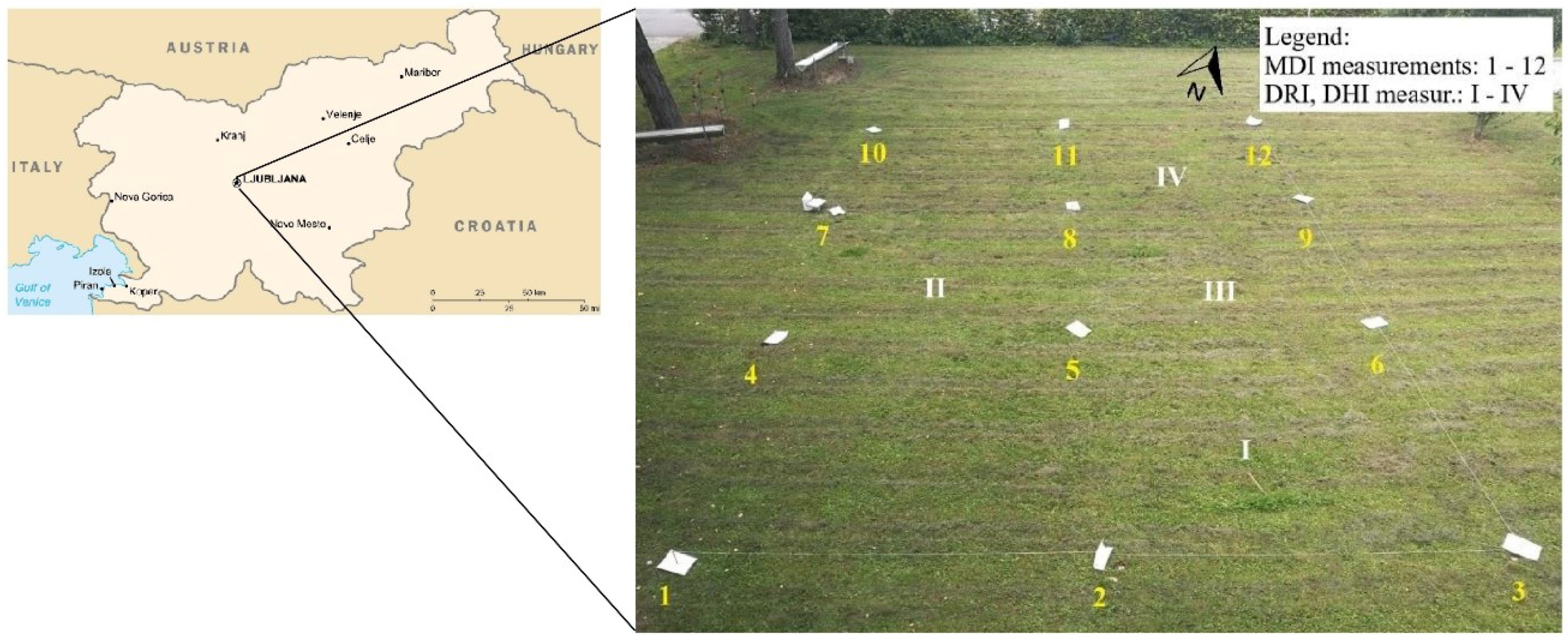
The study plot is located in an urban park in the city of Ljubljana, Slovenia (46°02’32.10’’ N, 14°29’33.50’’ E, 292 m a.s.l.), covering approximately 100 m2 and with a mean terrain slope of 1°. The typical climate for the area is temperate continental climate. The mean long-term (1986–2016) annual rainfall is approximately 1380 mm and the average annual temperature is 11 °C, ranging from −3 °C in the winter and 24 °C in the summer [19]. Plot is situated within an urbanized area of “Ljubljansko barje”, a marsh plain composed of mainly lacustrine and marsh Quaternary deposits of clay, silt, sand, gravel, and peat [20]. The natural type of soil in this area is Gleysol which is heavy-textured, dense and saturated with water long enough to develop reducing conditions [21]. However, as this is an urban area, soil map classifies it as “urban” (e.g., HAHT), offering no additional information on soil characteristics.
A grid of 3 × 4 measurement locations was set in the area, with a 4 m distance between locations in all directions, amounting to a study plot with dimensions of 8 × 12 m (Figure 1). Twelve locations within this grid were used for conducting measurements using MDI (yellow arabic numbers in Figure 1), whereas measurements using DRI and DHI were conducted in 4 locations (white roman numbers in Figure 1).
2.2. Soil Texture
Soil texture refers to the content of three main “fine earth” particle sizes in the soil according to their proportions in weight, which are sand, silt and clay; with next particle sizes for sand (0.05–2 mm), silt (0.002–0.05 mm) and clay (<0.002 mm) [22].
The main reasons for our field estimation of soil texture were two-fold. Firstly, it is a prerequisite for performing the DHI measurements, where different soil texture types determine the time and pressure head configurations of the instrument used. Secondly, soil texture is used to determine the fitting parameters for the DRI and MDI data analysis. Additionally, knowledge about soil texture can offer an approximate insight into the expected hydrologic characteristics and can also serve for determination of other infiltration model parameters as well as a control and reference for the data analysis, results, and interpretation [23].
The USDA classification scheme [22] was applied for soil texture estimation in the study, because of the readily available references for the field method, instrument parameter configuration and data analysis methods. In order to determine the soil texture class of soil samples taken from the locations I–IV, a field method (i.e., texture by feel analysis) was used. It is a qualitative method as it does not offer a detailed distribution of the different sizes soil particles by percent but instead focuses on determining only the rough ranges needed to assign a general soil texture class to the sampled soil. Thien [24] presented a simplified procedure of the method in the form of a flowchart, consisting of three main steps. In the first step, a 25 g soil sample is kneaded with the addition of water to achieve a suitable consistency for forming a ball. Then the ball is squeezed to form a ribbon and its length before it breaks from its own weight is recorded. In the final step, the soil sample is excessively wetted and felt for grittiness, smoothness, and stickiness, each corresponding to the prevailing texture class of the sampled soil.
2.3. Mini Disk Infiltrometer (MDI)
With a length of 32.7 cm and 135 mL of required water volume Mini disk infiltrometer (MDI) [25] is a practical version of a tension infiltrometer for conducting field measurements of unsaturated hydraulic conductivity (K); especially when having a limited access to water and on steep slopes. It is divided into two chambers, the top (bubble) chamber controls the suction applied to the disc, whereas the lower chamber contains a volume of water that infiltrates into the soil through a porous sintered stainless steel disk, at applied suction (0.5–7 cm) [25].
Method by Zhang [26] was applied to determine K based on measured cumulative infiltration. Results of the measurements are plotted on a graph, where the x-axis presents the square root of time and the y-axis presents cumulative infiltration. Afterwards, data points are fitted with a function (e.g., first two terms of the Philip’s infiltration equation [27]:
where I (cm) is the cumulative infiltration, C1 (cm/s1/2) is the soil sorptivity, C2 (cm/s) is parameter related to K and t is time (s). The hydraulic conductivity of the soil (K (cm/s)) is computed using the following equation:
where C2 is the slope of the curve of the cumulative infiltration versus square root of time and A2 is a value calculated using Equation (3):
where n and α are van Genuchten parameters determined for one of the 12 soil texture classes [28], r0 is the disk radius, h0 is the suction at the disk surface and c is a constant.
I = C1t1/2 + C2t
Method by Kutilek and Nielsen [29] was applied to estimate Ks (cm/s) from MDI measurements based on Equation (1):
where C1 (cm/s1/2) is sorptivity and m = 0.667.
I ≈ C1t1/2 + mKst
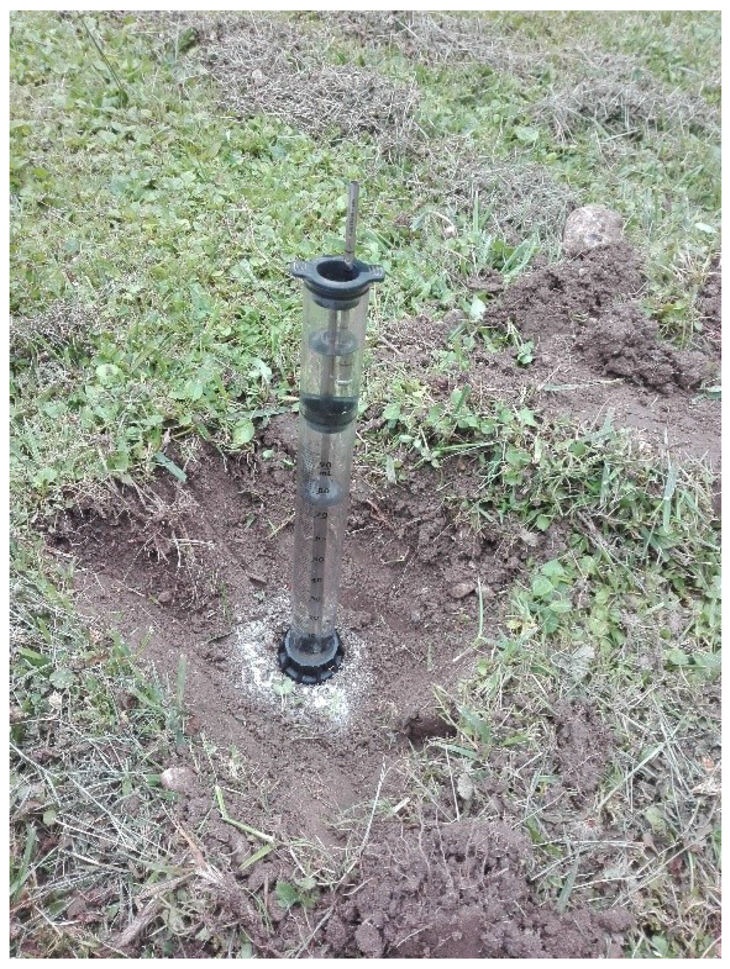
MDI measurements in the study were conducted under three different soil moisture conditions, namely dry (D), moist (M) and wet (W). Data on these conditions were obtained from Slovenian Environment Agency [30], which uses methodology based on World Meteorological Organization guide to determine state of the ground [31]. Measurements in dry conditions were conducted twice, on 20 July 2018 and 12 August 2018, in moist conditions on 24 July 2018, and in wet conditions on 14 August 2018. Two measurement series (20 July 2018, 24 July 2018) were conducted on the ground level (D0) as well as in a pit with depth of 10 cm (D10) (Figure 2) in order to identify possible influence of depth on measurement results. All together six series of measurements for all 12 locations (Figure 1) were conducted. Test ANOVA was applied to test the significance of differences between measurements conducted on the ground and in the pit.
To analytically find similarities/differences between locations, a method of hierarchical clustering by Orange software [32] was applied to MDI measurements. It forms a dendrogram for arbitrary types of objects based on a matrix of distances. Distances are calculated using Euclidian metric, which is the “ordinary” straight-line distance between two points in Euclidean space. To be more specific, distances are differences in measurement results between two locations overall series. For a better presentation of hierarchical clustering a distance map, which visualizes distances between objects, was applied. Namely, it replaces numbers presented in matrix of distances with coloured spots.
2.4. Double Ring Infiltrometer (DRI)
Double ring infiltrometer (DRI) [33] is designed to meet standards for conducting infiltration of water into soil in the field. It is an instrument used to determine Ks of the surface soil layer. DRI method is based on inserting inner (Ø 30 cm) and outer (Ø 60 cm) ring into the ground (10 cm deep), pouring water to initial level in both rings, recording the water level drop within the inner ring and measuring the time it takes for water to drop to a lower level. The process is repeated until the soil is saturated, i.e., the (quasi-steady) infiltration rate is the same for two consecutive tests. Based on the diameter of the inner ring and the time a certain level drop took, infiltration rate for observed time step can be determined.
Equation of USDA [34], which takes into account research conclusions from [35,36], was applied to calculate Ks from the observed steady infiltration rate:
where: Ks is the saturated hydraulic conductivity (cm/s), qs is the quasi-steady infiltration rate (cm/s), H is the steady depth of ponded water in ring (cm), a the inner ring radius (cm), d is the depth of ring insertion into the soil (cm), B1 and B2 are dimensionless quasi-empirical constants (for d > 3 and H > 5 cm: B1 = 0.316π, B2 = 0.184π), and α is the soil macroscopic capillary length (1/cm).
Soil macroscopic capillary length is estimated based on soil texture-structure categories [37] and was set to 0.12/cm, which is typical for most structured soils from clay through loams. Field measurements were conducted in dry conditions on 12 June 2018 at location II, 15 June 2018 at locations III and IV, 23 August 2018 at location III; in moist conditions on 27 August 2018 at location III and in wet conditions on 13 June 2018 at location I (Figure 1).
2.5. Dual Head Infiltrometer (DHI)
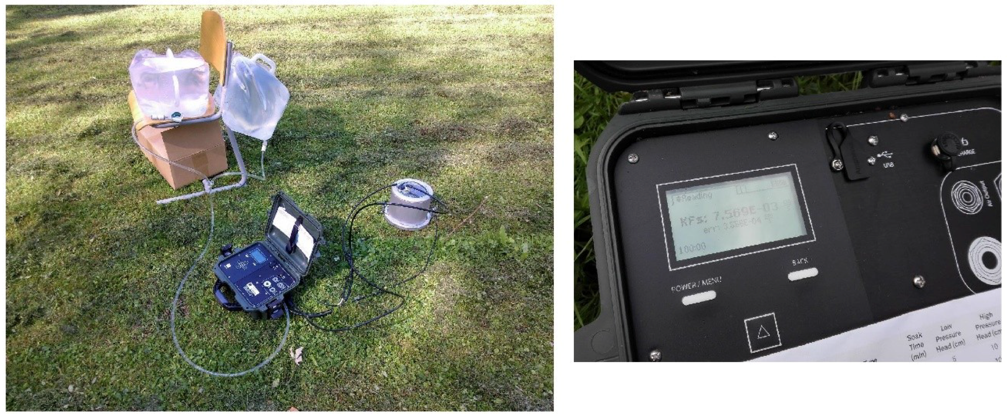
Dual head infiltrometer (DHI) SATURO [38] is essentially a single ring infiltrometer. It is capable of autonomous measurements via a peristaltic pump and water tanks with user input only before the start of testing. Depending on the expected infiltration rate connected to the soil texture at the analysed location, time and pressure parameter configuration is entered [38]. SATURO infiltrometer is a relatively recent instrument [39,40], with published results of measurements mainly in the field of ecohydrology [41,42,43].
Like all pressure infiltrometers, the DHI measures a three-dimensional infiltration process through a soil surface, where a ring is inserted to a certain depth and the soil is initially unsaturated [44]. For the purpose of data analysis, steady state ponded infiltration has to be assumed in order to use the common method [35], which is based on this assumption even though a true steady state is rarely achieved in natural, nonhomogeneous materials and the term quasi-steady-state is more suitable. The DHI uses the two-ponding head approach by Reynolds & Elrick [35], who provided an analytical equation for three-dimensional steady flow from the ring infiltrometer, accounting for its three main components: hydrostatic pressure of the ponded head, capillarity of the unsaturated soil, and gravity. The technique used is the bottomless bucket method after Nimmo [45], where falling-head infiltration is introduced following the achieved steady-state infiltration. Firstly, the infiltration rate is measured at one pressure head, and then the pressure head is lowered. The final Ks value is the average of infiltration rates at both pressure head cycles. With modifications of the original analytical equation, the dependence of the final field Ks result on soil characteristics is eliminated and only the pressure head data and infiltration rates are used for its calculation, which becomes:
where Δ is the infiltrometer geometry constant, i are the infiltration rates at their appropriate pressure heads and D symbols the different pressure heads, their values represented by the averages for each of the pressure cycles. Apart from the Ks value, the result of the DHI test also includes a standard error, representing the amount of noise in the measurements that were averaged. For the locations I-IV on the study plot (Figure 1), DHI was applied for characterizing the hydraulic characteristics of the soil apart from the DRI. Field measurements were conducted on 19 September 2018 in dry conditions at locations I, II, IV and on 18 October 2018 in wet conditions at location III (Figure 3). The chosen parameter configuration was the same for all four measurements and included a 5 cm low- and 10 cm high-pressure head, 20 min of soak time and 2 cycles of 20 min time for each pressure head.
3. Results and Discussion
3.1. Soil Texture
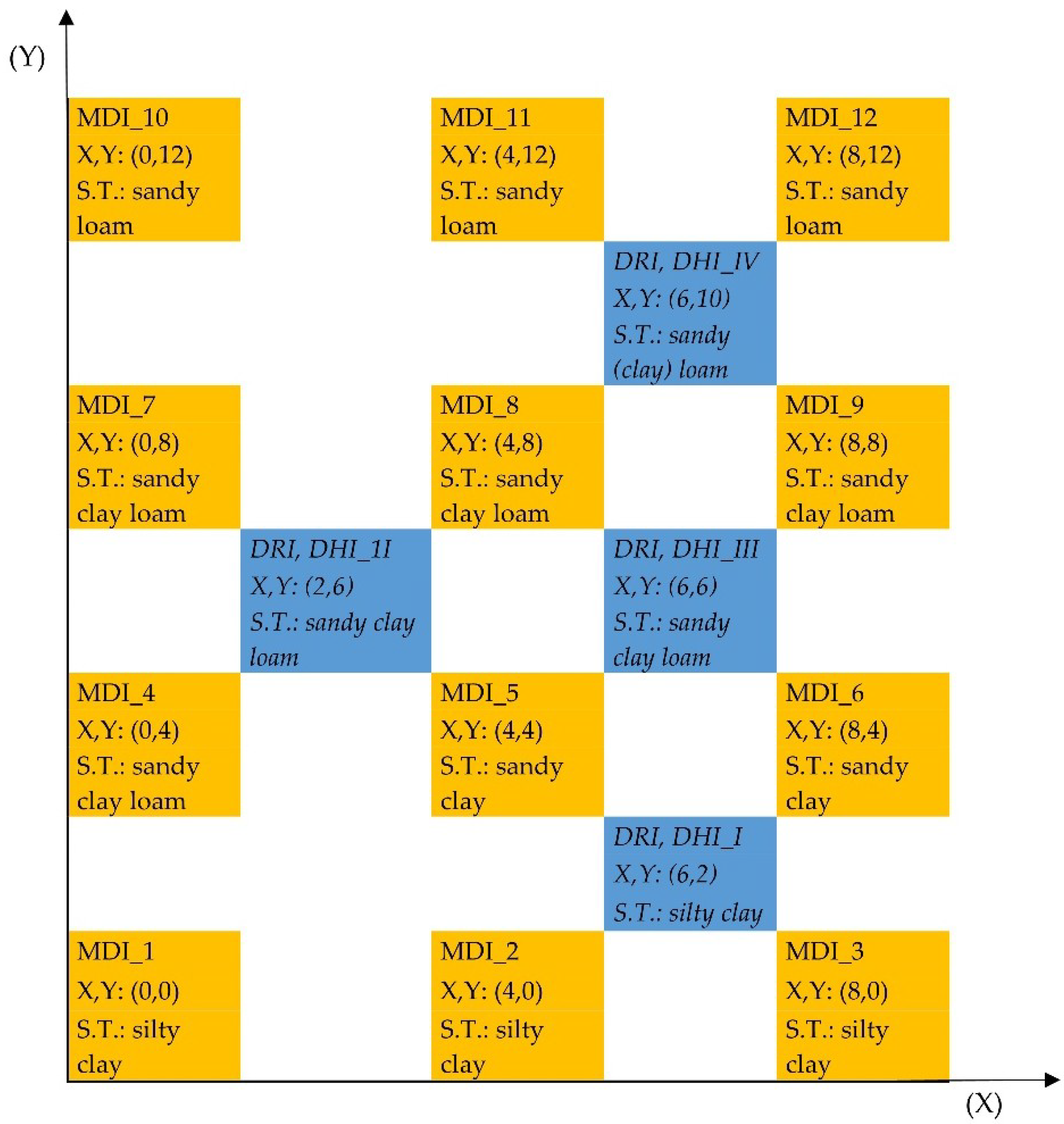
Soil texture for locations I–IV (Figure 4), where DRI and DHI measurements were conducted was determined by the so-called texture by feel analysis. According to so defined soil texture at DRI and DHI measurement locations (I–IV), soil texture for MDI measurement at locations 1–12 was determined. Estimated soil textures vary from sandy loam at the north part of the study plot, transitioning to sandy clay loam in the middle, and silty clay at the south part of the study plot.
3.2. Mini Disk Infiltrometer (MDI)
Six series of measurements for all 12 locations were conducted with MDI. Average K (cm/s), standard deviation (St. dev.) (cm/s), and coefficient of variation (CV) (%) were calculated for MDI measurements for all 12 locations (Table 1).
The first measurement series (No. 1 - K_D_D0_12.8.18) was excluded from statistical analysis of temporal variability for MDI locations, since multiple measurements were conducted in dry soil conditions. Furthermore, this series stands out with the lowest measured K values (i.e., on average 10–20 times lower), when compared to other series. This can be explained with a phenomenon of water repellency caused by a very dry period, where no significant precipitation was measured since 3 August 2018 (total precipitation 29.5 mm) that reduced K. This phenomena was also observed by other researchers (e.g., [46,47,48]), reporting that low water content and high temperatures induce soil water repellency. This is not a fixed condition of the soil and can be diminished with influx of water that increases water content in the soil [49,50]. Das Gupta, Mohanty, and Köhne [13] reported that K in Vertisol soil, with high clay minerals content, was positively correlated with antecedent moisture contents at soil water pressure heads close to saturation, reflecting liquid cohesion, water films bridging across different crack-separated peds, and activation of flow in structural and biological macropores in the bioporous soil system.
K varies significantly between locations (i.e., coefficient of variation (CV) ranges from 33% to 89%). Apart from the most homogenous series (No. 6.), spatial variation is even higher, namely 67% to 89%. Significant spatial variability of K was also reported by other authors (e.g., [51,52,53]).
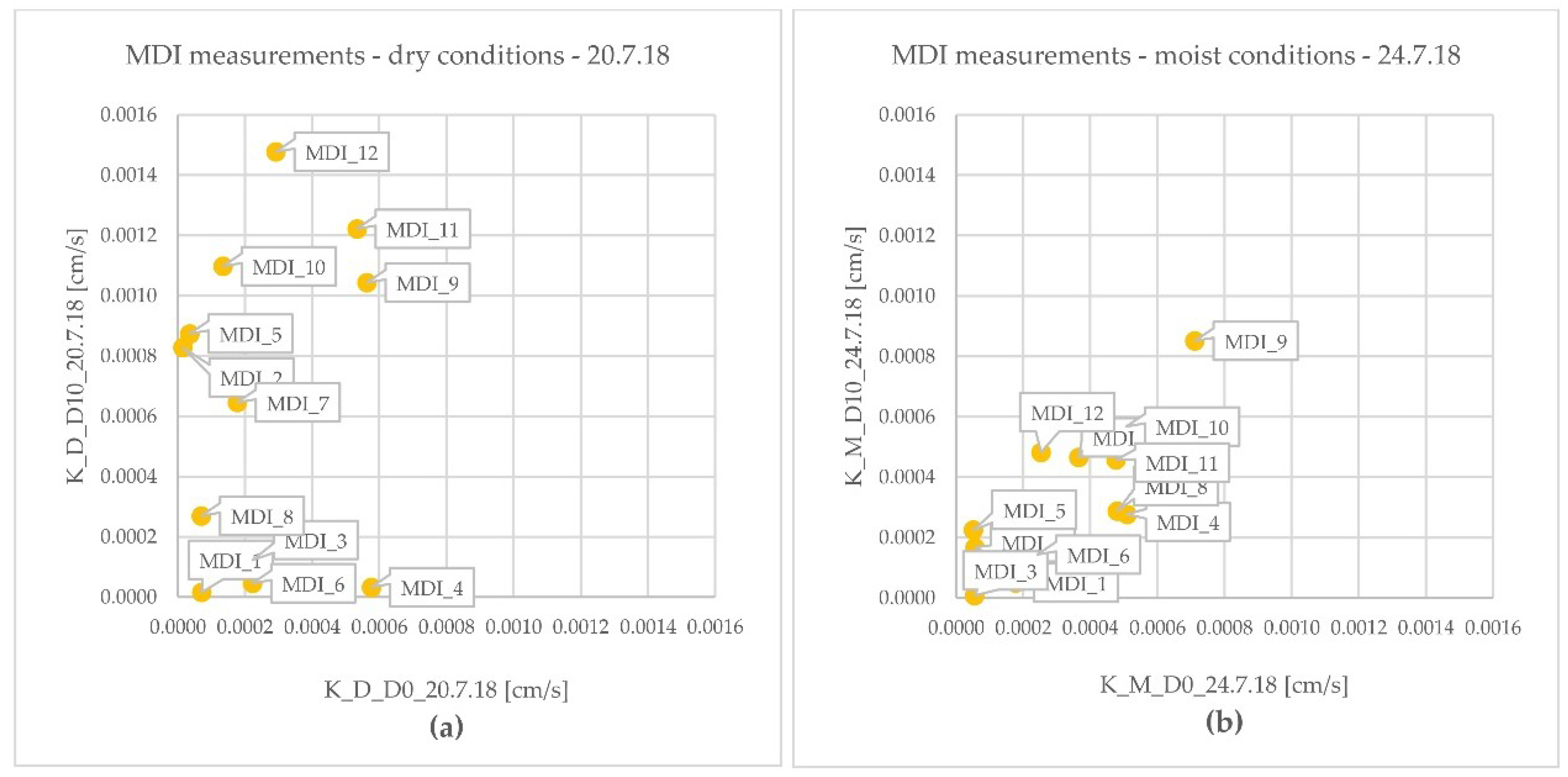
MDI measurements on 20 July 2018 (dry conditions) and 24 July 2018 (wet conditions) were conducted on the ground level (0 cm deep—D0) as well as in a pit with depth of 10 cm (D10). K in a freshly dug pit was higher compared to K measured at ground level (Figure 5a). Moreover, ANOVA test demonstrated that the differences between the series means were statistically significant (p-value 0.023) at the significance level of 0.05. The soil in the pit was not exposed to the drying process to the same extent as the soil on the ground; hence the water repellency was not as strong. Measurements resulted in similar K on both levels when the pit was exposed to the same weather conditions as the ground level for 4 days (Figure 5b). Additionally, ANOVA test demonstrated that the differences between the series means were not statistically significant (p-value 0.935) at the significance level of 0.05.
In order to investigate the magnitude of the spatial and temporal variability of K within the study plot, results of the MDI measurements were presented using heat maps (Figure 6). Linear interpolation was applied to calculate K values among the measurement points. It can be depicted that the lowest K and the most homogenous results in absolute terms (the lowest St. dev.) were measured on 12 August 2018, caused by water repellency effect (Figure 6a). K was approx. 3 times higher for the measurements conducted in a freshly dug pit compared to ground level measurements conducted on same day (20 July 2018) (Figure 6b). After 4 days of exposure to weather conditions, average K was very similar on both levels (Figure 6c). Although the measurements on 14 August 2018 were conducted in wet conditions, the highest K and the most homogenous results in relative terms (lowest CV) among ground level measurements were observed (Figure 6d).
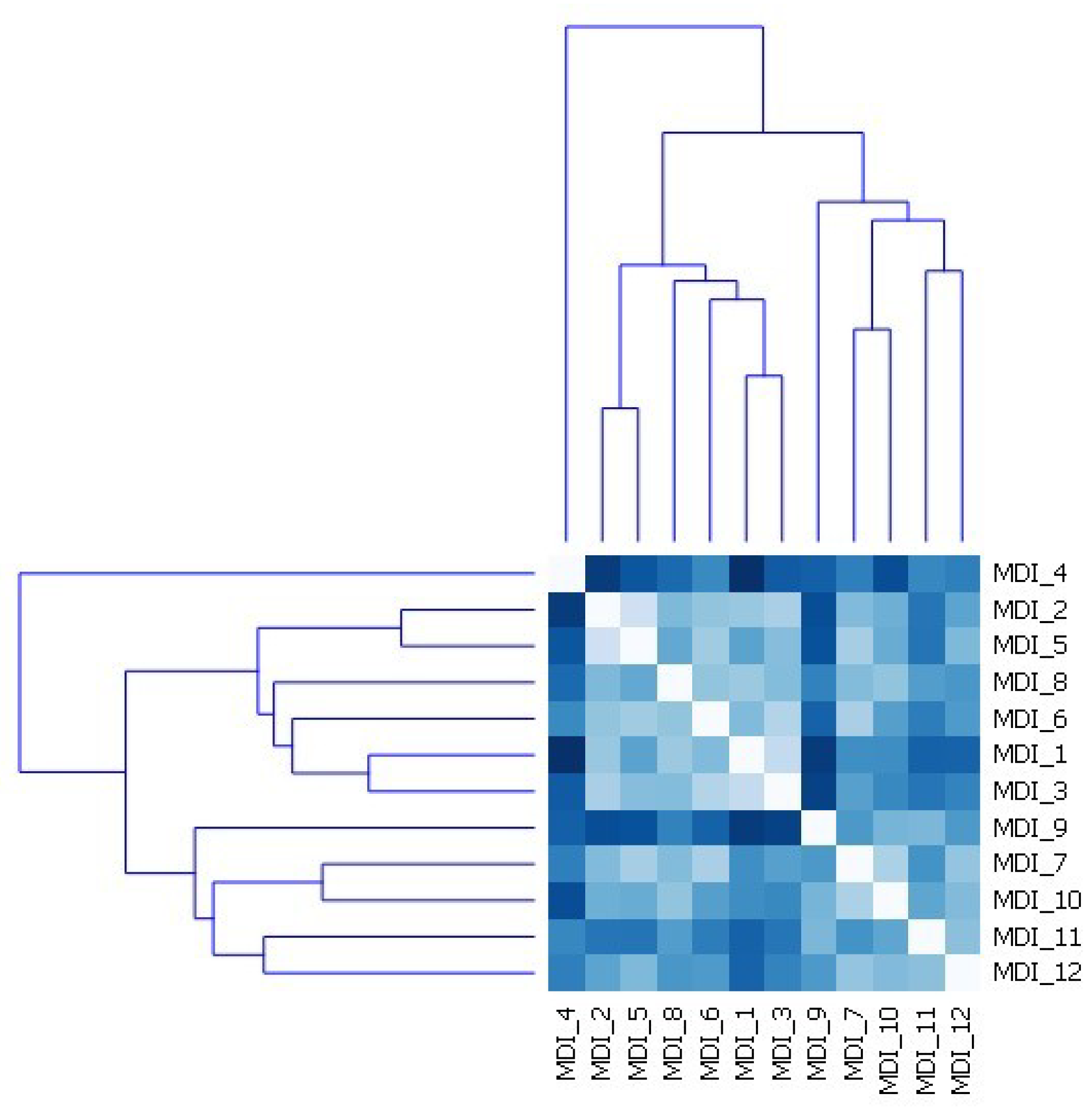
MDI measurement results presented in Table 1 were applied in the hierarchical clustering, considering all six series of measurements at all 12 locations. Results demonstrate that measurement locations can be clustered into two major groups (Figure 7). The southern two rows of the study plot form one group (locations: 1,2,3,4,5,6,8) and the northern two rows form a second group (locations: 7,9,10,11,12). The exception is location MDI_8 that was placed in the southern group, instead of northern group.
A distance map of MDI measurement results was formed (Figure 7), where dark blue colour presents the largest differences in distances between locations and white colour the smallest differences or a match. Two locations clearly stand out with the highest differences in distances, namely MDI_4 and MDI_9. Averaged results of MDI measurements over series No. 2–No. 6 (Table 1), show that these two measurement locations have the highest averages within their groups. In consequence, these results point to the spatial variability of K and to the need of conducting a sufficient number of measurements to identify outlier locations.
3.3. Double Ring Infiltrometer (DRI)
DRI measurements confirm the soil texture types determined with the soil texture analysis by feel. Ks is increasing from location I to location IV (Table 2), similarly soil texture changes from less (i.e., silty clay) to more permeable soil (i.e., sandy (clay) loam). Additionally, multiple measurements were conducted at location III to access their reliability. This location was chosen as it lays in the centre of the study plot, in-between other three locations. Two measurements were conducted in dry conditions (15 June 2018, 23 August 2018), resulting in similar results, with an average Ks of 0.86 (±0.02) × 10−3 cm/s, whereas third measurement (27 August 2018) was conducted in wet conditions, resulting in lower Ks of 0.5 × 10⁻³ cm/s.
3.4. Dual Head Infiltrometer (DHI)
Following values of Ks (× 10−3 cm/s) were measured using DHI on locations from I to IV: (I) 1.2 (± 0.04), (II) 8.8 (± 0.3), (III) 7.6 (± 0.4), (IV) 17.7 (± 0.5). As in the case of DRI measurements, DHI measurements demonstrate an increase of Ks values in the direction from location I to IV (Table 2), following the transition from finer to coarser soil textures (Figure 4).
3.5. Comparison of the Results of Applied Measurement Techniques
To compare DRI and DHI results (e.g., Ks) with results obtained by MDI (e.g., K), Equation (4) was used to estimate Ks from MDI measurements. Additionally, MDI values for locations I-IV were calculated as an average of the MDI measurements at the surrounding four locations (e.g., for location I, results at locations 2,3,5,6 were used) (Table 2).
The results demonstrate that DHI measured the highest average Ks (8.2 ± 5.9 × 10⁻³ cm/s), followed by MDI (2.6 ± 0.5 × 10⁻³ cm/s) and the lowest Ks was measured by DRI (1.0 ± 1.1 × 10⁻³ cm/s) (Table 2). When comparing measurement results, the best match between both instruments that measure Ks (DHI and DRI) is expected. This was not true in our case, since DHI measurements were on average 6.8 times higher than DRI measurements. To our best knowledge, only Rivera [54] published a case report where these two methods were compared. He conducted measurements on a turf field with seven locations. Five of them achieved a good fit, but two parallel locations, showed significant differences, where DHI measurements had higher Ks. Authors of the study hypothesised that the amount of force required to install DRI disturbed the structure of the soil and crushed the macropores. Because of this disturbance, the field Ks from the DRI was two factors of difference lower than the DHI measurements. Above mentioned is one of the plausible reasons for the observed result differences in our study. Furthermore, differences could be induced also by lower impact of smaller ring installation (i.e., a smaller portion of soil is saturated) in the case of DHI compared to DRI.
The most comparable results for Ks were obtained with MDI and DRI, with factor of difference of 2.7. Ghosh and Pekkat [16] reported that hydraulic conductivity determined by MDI were approximately 0.5 to 0.67 of DRI values. When comparing K obtained with MDI to Ks obtained with DRI similar ratios were observed in this study (Table 2).
Fodor et al. [11] investigated dependency of measuring methods on hydraulic conductivity. Among applied instruments were MDI (measures hydraulic conductivity of the soil matrix) and DRI (measures hydraulic conductivity including macro-pore flow). DRI resulted in higher K for sand (1.0 × 10⁻³ cm/s), but lower K for silt loam (0.9 × 10⁻³ cm/s) and vice-versa for MDI (sand: 0.9 × 10⁻³ cm/s, silt loam: 1.5 × 10⁻³ cm/s). Showing that predominance of a soil matrix or a macro-pore flow depends on the investigated type of soil. In our case, macro-pore flow (Ks) increases significantly (with factor 10) from location I (sandy silty clay) towards location IV (sandy clay loam), whereas soil matrix flow (K) increases moderately (with factor 2).
Measurement results were compared with reference Ks values, provided in Soil Survey Manual by USDA [22], which are estimated based on soil texture type and bulk density. Considering that investigated soils correspond to a medium density bulk class, measured Ks values obtained with DRI are generally in line with the reference values. Namely, Ks should range between 0.1–1 × 10⁻³ cm/s for sandy clay loam (SCL) (locations II and III) and between 1–10 × 10−3 cm/s for sandy loam (SL) (location IV). On the other hand, measurement results obtained at location I (0.4 × 10⁻³ cm/s), correspond better to the reference values for silty loam (SiL) (0.1–1 × 10⁻³ cm/s) texture class, than silty clay (SiC) (0.001–0.01 × 10⁻³ cm/s), which was determined with analysis by feel (i.e., qualitative assessment). If SiL would be used instead of SiC as a reference soil texture type for location I, this would not have any influence on DHI and DRI results. Namely, the same parameter configuration was used to undertake DHI measurements for all four locations and the same value of α (soil macroscopic capillary length) was used in Equation (5) to evaluate all DRI measurements. However, using SiL instead of SiC would lead to minor reductions (approx. 13%) of K values obtained by MDI at location I. This indicates that analysis by feel should primarily be used as the first approximation to determine soil texture class, while values that are more accurate should be estimated by laboratory analysis.
3.6. Infiltration and Urban Drainage Modelling
Infiltration is one of the key processes in urban drainage modelling and stormwater control measures design. Therefore, proper estimation of soil hydraulic conductivity is of high importance. Petrucci, De Bondt, and Claeys [9] proposed an improvement of infiltration regulations towards more effective urban stormwater management. Namely, homogenous regulations applying uniform soil characteristics can cause superfluous storage or miss the whole infiltration potential. In contrast, heterogeneous regulations, which take into account plot specific soil characteristics, can be more effective. Furthermore, the regulations demanding local tests for determining Ks take into account its spatial variability, but not its temporal variability. Presented findings indicate that hydrological models could be enhanced using different scenarios by employing a range of K values (lower and upper bound) that vary based on soil conditions (e.g., dry, moist, wet), instead of taking a constant value for K. Moreover, MDI proved to be a useful quick method for multiple measurements of K under different weather conditions.
4. Conclusions
In this study, three techniques, namely mini disk infiltrometer (MDI), double ring infiltrometer (DRI), and dual head infiltrometer (DHI) were applied to identify spatial in temporal variability of (un)saturated hydraulic conductivity of soils in an urban setting in the City of Ljubljana, Slovenia. General conclusions:
- Both methods for measuring Ks (DHI and DRI) show an increase in its value, when moving from locations with silty clay towards locations with sandy loam soil pointing to spatial variability of Ks within a limited space. On average, results of Ks using DHI are 6.8 times higher than when using DRI;
- Multiple measurements using DRI at the same location (III) under different weather conditions (i.e., dry and wet) highlighted the temporal variability of Ks;
- Although DRI and MDI measure different types of hydraulic conductivity, their values are the most similar after estimation of Ks for MDI (i.e., results of DRI are 2.7 times higher than MDI).
Related to the MDI measurements following conclusions can be drawn:
- MDI measurements pointed to the spatial variability of K, with coefficient of variation ranging from 67%–89% over five measurement series. Furthermore, looking at average K for every MDI location, these vary from 11 to 73 × 10−5 cm/s, with a high coefficient of temporal variability (27%–99%);
- When exposed to drought, water repellency was formed in soil, leading to the lowest measured average K (2.6 × 10⁻⁵ cm/s). After a rain event, water repellency was diminished, establishing a normal average K (54.7 × 10⁻⁵ cm/s), with a small coefficient of variability (33%). This clearly showed the magnitude of temporal variability of K;
- MDI measurements demonstrated that under dry conditions K was on average three times higher in a freshly dug pit than on the ground level. The test was repeated after four days when conditions on both levels became similar. Previously observed difference diminished, resulting in almost the same value of average K (33 × 10−5 cm/s) in the pit and on the ground. This reinforces the theory of water repellency formation in the top soil under dry and warm weather conditions.
Following all presented results in the observed urban catchment, the magnitude of spatial and temporal variability of K was identified. Moreover, measurement results significantly varied between the three investigated techniques. The site-specific relationships among the results of all three used techniques were identified. To the best of our knowledge, this is the first study that compared measurements results between MDI, DRI, and DHI. Over time, conducting similar comparisons in different locations and conditions will enable to derive a general relationship between method results, similar to what was reported by Ghosh and Pekkat [16] for comparison of MDI and DRI results. The presented findings should be considered in the development of UD models and especially in the design of infiltration-based SCMs in urban catchments.
Author Contributions
All authors conceptualized the research problem and formulated goals and aims of the study; N.A. and M.R. elaborated the connection between hydraulic conductivity and SCM; M.M. helped with the selection and provision of field equipment; M.R. and I.V. collected and analysed the soil hydraulic conductivity data; M.R. conducted data visualization; M.Š. oversaw and lead the research activity planning and execution; All authors contributed to the interpretation of the results, manuscript writing and revision.
Funding
The authors acknowledge the financial support from the Slovenian Research Agency (research core funding No. P2-0180) through the PhD grant of the first author (M. Radinja).
Conflicts of Interest
The authors declare no conflict of interest. The funders had no role in the design of the study; in the collection, analyses, or interpretation of data; in the writing of the manuscript, or in the decision to publish the results.
References
- Butler, D.; James Digman, C.; Makropoulos, C.; Davies, J. Urban Drainage, 4th ed.; CRC Press: Boca Raton, FL, USA, 2018. [Google Scholar]
- Radinja, M.; Banovec, P.; Comas Matas, J.; Atanasova, N. Modelling and Evaluating Impacts of Distributed Retention and Infiltration Measures on Urban Runoff. Acta Hydrotech. 2017, 30, 51–64. [Google Scholar]
- Šraj, M.; Dirnbek, L.; Brilly, M. The influence of effective rainfall on modelled runoff hydrograph. J. Hydrol. Hydromech. 2010, 58, 3–14. [Google Scholar] [CrossRef]
- Rossman, L. Storm Water Management Model User’s Manual Version 5.1; US EPA Office of Research and Development: Washington, DC, USA, 2015.
- Duan, W.; He, B.; Takara, K.; Luo, P.; Nover, D.; Hu, M. Impacts of climate change on the hydro-climatology of the upper Ishikari river basin, Japan. Environ. Earth Sci. 2017, 76, 490. [Google Scholar] [CrossRef]
- Zhou, Q. A Review of Sustainable Urban Drainage Systems Considering the Climate Change and Urbanization Impacts. Water 2014, 6, 976–992. [Google Scholar] [CrossRef] [Green Version]
- Fletcher, T.D.; Shuster, W.; Hunt, W.F.; Ashley, R.; Butler, D.; Arthur, S.; Trowsdale, S.; Barraud, S.; Semadeni-Davies, A.; Bertrand-Krajewski, J.L.; et al. SUDS, LID, BMPs, WSUD and more—The evolution and application of terminology surrounding urban drainage. Urban Water J. 2015, 12, 525–542. [Google Scholar] [CrossRef]
- Gadi, V.K.; Tang, Y.-R.; Das, A.; Monga, C.; Garg, A.; Berretta, C.; Sahoo, L. Spatial and temporal variation of hydraulic conductivity and vegetation growth in green infrastructures using infiltrometer and visual technique. Catena 2017, 155, 20–29. [Google Scholar] [CrossRef] [Green Version]
- Petrucci, G.; De Bondt, K.; Claeys, P. Toward better practices in infiltration regulations for urban stormwater management. Urban Water J. 2017, 14, 546–550. [Google Scholar] [CrossRef]
- Deb, S.K.; Shukla, M.K. Variability of hydraulic conductivity due to multiple factors. Am. J. Environ. Sci. 2012, 8, 489–502. [Google Scholar] [CrossRef]
- Fodor, N.; Sándor, R.; Orfanus, T.; Lichner, L.; Rajkai, K. Evaluation method dependency of measured saturated hydraulic conductivity. Geoderma 2011, 165, 60–68. [Google Scholar] [CrossRef]
- Kanso, T.; Tedoldi, D.; Gromaire, M.-C.; Ramier, D.; Saad, M.; Chebbo, G. Horizontal and Vertical Variability of Soil Hydraulic Properties in Roadside Sustainable Drainage Systems (SuDS)—Nature and Implications for Hydrological Performance Evaluation. Water 2018, 10, 987. [Google Scholar] [CrossRef]
- Das Gupta, S.; Mohanty, B.P.; Köhne, J.M. Soil Hydraulic Conductivities and their Spatial and Temporal Variations in a Vertisol. Soil Sci. Soc. Am. J. 2006, 70, 1872–1881. [Google Scholar] [CrossRef]
- Bockhorn, B.; Klint, K.E.S.; Locatelli, L.; Park, Y.-J.; Binning, P.J.; Sudicky, E.; Bergen Jensen, M. Factors affecting the hydraulic performance of infiltration based SUDS in clay. Urban Water J. 2017, 14, 125–133. [Google Scholar] [CrossRef]
- Galbraith, J.M. Human-altered and human-transported (HAHT) soils in the U.S. soil classification system. Soil Sci. Plant Nutr. 2018, 64, 190–199. [Google Scholar] [CrossRef]
- Ghosh, B.; Pekkat, S. A critical evaluation of measurement-induced variability in infiltration characteristics for a river sub-catchment. Measurement 2019, 132, 47–59. [Google Scholar] [CrossRef]
- Robichaud, P.R.; Lewis, S.; Ashmun, L. New Procedure for Sampling Infiltration to Assess Post-fire Soil Water Repellency; Research Note RMRS-RN-33; U.S. Department of Agriculture, Forest Service, Rocky Mountain Research Station: Fort Collins, CO, USA, 2008.
- Köhne, J.M.; Júnior, J.A.; Köhne, S.; Tiemeyer, B.; Lennartz, B.; Kruse, J. Double-ring and tension infiltrometer measurements of hydraulic conductivity and mobile soil regions. Pesqui. Agropecu. Trop. 2011, 41, 336–347. [Google Scholar]
- ARSO Meteorological Achive. Available online: http://www.meteo.si/met/sl/archive/ (accessed on 5 July 2018).
- Premru, U. Tolmač za list Ljubljana: L 33-66. Osnovna geološka karta SFRJ 1: 100 000 ([Interpretation of sheet Ljubljana: L 33-66. Elementary geological map SFRJ 1: 100 000]; Zvezni geološki zavod: Belgrade, Serbia, 1983. [Google Scholar]
- Vrščaj, B.; Kralj, T. Slovenian soil classification and WRB. In The Soils of Slovenia; Springer: Berlin, Germany, 2017; ISBN 9789401785846. [Google Scholar]
- USDA. Soil Survey Manual; Government Printing Office: Washington, DC, USA, 2017; ISBN 978-1410204172.
- Ritchey, E.L.; Mcgrath, J.M.; Gehring, D. Determining Soil Texture by Feel; Agriculture and Natural Resources Publication 139; University of Kentucky, College of Agriculture, Food and Environment: Lexington, KY, USA, 2015. [Google Scholar]
- Thien, S.J. A flow diagram for teaching texture-by-feel analysis. J. Agron. Educ. 1979, 8, 54–55. [Google Scholar]
- METER Group Inc. Mini Disk Infiltrometer; METER Group Inc.: Pullman, WA, USA, 2018. [Google Scholar]
- Zhang, R. Determination of Soil Sorptivity and Hydraulic Conductivity from the Disk Infiltrometer. Soil Sci. Soc. Am. J. 1997, 61, 1024–1030. [Google Scholar] [CrossRef]
- Philip, J.R. The theory of infiltration: 1. The infiltration equation and its solution. Soil Sci. 1957, 83, 345–358. [Google Scholar] [CrossRef]
- Carsel, R.F.; Parrish, R.S. Developing joint probability distributions of soil water retention characteristics. Water Resour. Res. 1988, 24, 755–769. [Google Scholar] [CrossRef]
- Kutilek, M.; Nielsen, D.R. Soil Hydrology; Catena-Verlag: Cremlingen-Destedt, Germany, 1994. [Google Scholar]
- ARSO Temperature and Condition of Soil. Available online: http://meteo.arso.gov.si/met/sl/agromet/recent/tsoil (accessed on 5 July 2018).
- Guide to Meteorological Instruments and Methods of Observation; WMO-No. 8; World Meteorological Organization: Geneva, Switzerland, 2012.
- Demšar, J.; Curk, T.; Erjavec, A.; Hočevar, T.; Milutinovič, M.; Možina, M.; Polajnar, M.; Toplak, M.; Starič, A.; Štajdohar, M.; et al. Orange: data mining toolbox in Python. J. Mach. Learn. Res. 2013, 14, 2349–2353. [Google Scholar]
- Double Ring Infiltrometer Manual; Eijkelkamp: Giesbeek, The Netherlands, 2015.
- Soil Survey Staff. Soil Survey Field and Laboratory Methods Manual; U.S. Department of Agriculture, Natural Resources Conservation Service: Lincoln, NE, USA, 2014.
- Reynolds, W.D.; Elrick, D.E. Ponded Infiltration From a Single Ring: I. Analysis of Steady Flow. Soil Sci. Soc. Am. J. 1990, 54, 1233–1241. [Google Scholar] [CrossRef]
- Youngs, E.G.; Leeds-Harrison, P.B.; Elrick, D.E. The hydraulic conductivity of low permeability wet soils used as landfill lining and capping material: analysis of pressure infiltrometer measurements. Soil Technol. 1995, 8, 153–160. [Google Scholar] [CrossRef]
- Elrick, D.E.; Reynolds, W.D.; Tan, K.A. Hydraulic Conductivity Measurements in the Unsaturated Zone Using Improved Well Analyses. Groundw. Monit. Remediat. 1989, 9, 184–193. [Google Scholar] [CrossRef]
- METER Group Inc. SATURO; METER Group Inc.: Pullman, WA, USA, 2017. [Google Scholar]
- Wacker, K.; Campbell, G.; Rivera, L. An Automated Dual-Head Infiltrometer for Measuring Field Saturated Hydraulic Conductivity Dual-head Infiltrometer Equations; Decagon Devices Inc.: Pullman, WA, USA, 2009. [Google Scholar]
- Cobos, D.; Rivera, L.; Campbell, G. Automated Dual-Head Infiltrometer for Measuring Field Saturated Hydraulic Conductivity (Kfs). Geophys. Res. Abstr. 2015, 17, EGU2015-14348. [Google Scholar]
- Demirtas, I. Effects of Post-Fire Salvage Logging on Compaction, Infiltration, Water Repellency, and Sediment Yield and the Effectiveness of Subsoiling on Skid Trails. Master’s Thesis, Michigan Technological University, Houghton, MI, USA, 2017. [Google Scholar]
- Gonzales, H.B.; Ravi, S.; Li, J.; Sankey, J.B. Ecohydrological implications of aeolian sediment trapping by sparse vegetation in drylands. Ecohydrology 2018, 11, e1986. [Google Scholar] [CrossRef]
- Ravi, S.; Wang, L.; Kaseke, K.F.; Buynevich, I.V.; Marais, E. Ecohydrological interactions within “fairy circles” in the Namib Desert: Revisiting the self-organization hypothesis. J. Geophys. Res. Biogeosci. 2017, 122, 405–414. [Google Scholar] [CrossRef] [Green Version]
- Angulo-Jaramillo, R.; Bagarello, V.; Iovino, M.; Lassabatere, L. Infiltration Measurements for Soil Hydraulic Characterization; Springer International Publishing: Cham, Switzerland, 2016; ISBN 9783319317885. [Google Scholar]
- Nimmo, J.R.; Schmidt, K.M.; Perkins, K.S.; Stock, J.D. Rapid Measurement of Field-Saturated Hydraulic Conductivity for Areal Characterization. Vadose Zone. J. 2009, 8, 142–149. [Google Scholar] [CrossRef]
- Lucas-Borja, M.E.; Zema, D.A.; Plaza-Álvarez, P.A.; Zupanc, V.; Baartman, J.; Sagra, J.; González-Romero, J.; Moya, D.; de las Heras, J. Effects of Different Land Uses (Abandoned Farmland, Intensive Agriculture and Forest) on Soil Hydrological Properties in Southern Spain. Water 2019, 11, 503. [Google Scholar] [CrossRef]
- DeBano, L.F. Water Repellent Soils: A State-of-the-art; General Technical Report PSW-GTR-46; U.S. Department of Agriculture, Forest Service, Pacific Southwest Forest and Range Experiment Station: Berkeley, CA, USA, 1981.
- Debano, L.F. Water repellency in soils: A historical overview. J. Hydrol. 2000, 231–232, 4–32. [Google Scholar] [CrossRef]
- de Jonge, L.W.; Jacobsen, O.H.; Moldrup, P. Soil Water Repellency: Effects of Water Content, Temperature, and Particle Size. Soil Sci. Soc. Am. J. 1999, 63, 437. [Google Scholar] [CrossRef]
- Leelamanie, D.A.L.; Karube, J. Effects of organic compounds, water content and clay on the water repellency of a model sandy soil. Soil Sci. Plant Nutr. 2007, 53, 711–719. [Google Scholar] [CrossRef] [Green Version]
- Stolte, J.; Van Venrooij, B.; Zhang, G.; Trouwborst, K.O.; Liu, G.; Ritsema, C.J.; Hessel, R. Land-use induced spatial heterogeneity of soil hydraulic properties on the Loess Plateau in China. Catena 2003, 54, 59–76. [Google Scholar] [CrossRef]
- Lichner, L.; Orfánus, T.; Nováková, K.; Miloslav, Š.Í.R.; Tesař, M. The impact of vegetation on hydraulic conductivity of sandy soil. Soil Water Res. 2007, 2, 59–66. [Google Scholar] [CrossRef]
- Zhou, X.; Lin, H.S.; White, E.A. Surface soil hydraulic properties in four soil series under different land uses and their temporal changes. Catena 2008, 73, 180–188. [Google Scholar] [CrossRef]
- Rivera, L.D. Comparing the Automated Dual-Head Analysis from a Single-Ring Infiltrometer with a Double-Ring Infiltrometer. In Proceedings of the Managing Global Resources for a Secure Future, 2017 Annual Meeting, Tampa, FL, USA, 22–25 October 2017; pp. 1–4. [Google Scholar]
Figure 1.
Study plot with measurement locations.

Figure 2.
Mini disk infiltrometer (MDI) measurement in a pit with depth of 10 cm (D10).

Figure 3.
Field measurements of Ks using dual head infiltrometer (DHI) on the study plot and DHI screen.
Figure 3.
Field measurements of Ks using dual head infiltrometer (DHI) on the study plot and DHI screen.

Figure 4.
Soil texture (S.T.) at measurement locations.

Figure 5.
Scatter plots of MDI measurements conducted on the ground and in the pit. (a) K_D_D0_20.7.18; (b) K_M_D0_24.7.18.
Figure 5.
Scatter plots of MDI measurements conducted on the ground and in the pit. (a) K_D_D0_20.7.18; (b) K_M_D0_24.7.18.

Figure 6.
Results of MDI measurements presented using heat maps.

Figure 7.
Distance map of hierarchical clustering of MDI measurement results (darker the colour the larger difference).
Figure 7.
Distance map of hierarchical clustering of MDI measurement results (darker the colour the larger difference).


Table 1.
Results of MDI measurements.
| MEASUREMENT SERIES | TEMPORAL VARIAB. | |||||||||
|---|---|---|---|---|---|---|---|---|---|---|
| No. 1 | No. 2 | No. 3 | No. 4. | No. 5 | No. 6 | Aver. | St. dev. | CV | ||
| K_D_D0 _12.8.18 | K_D_D0 _20.7.18 | K_D_D10 _20.7.18 | K_M_D0 _24.7.18 | K_M_D10 _24.7.18 | K_W_D0 _14.8.18 | without No. 1 | ||||
| (× 10−5 cm/s) | (× 10−5 cm/s) | (%) | ||||||||
| MDI LOCATION | MDI_1 | 0.5 | 7.1 | 1.6 | 17.7 | 5 | 25.5 | 11.4 | 8.9 | 78% |
| MDI_2 | 0.8 | 1.4 | 82.8 | 5.6 | 16.7 | 49 | 31.1 | 30.8 | 99% | |
| MDI_3 | 1.8 | 22.3 | 12.3 | 5.5 | 0.8 | 42.2 | 16.6 | 14.7 | 88% | |
| MDI_4 | 8 | 57.6 | 3.3 | 51 | 27.7 | 87.1 | 45.4 | 28.3 | 62% | |
| MDI_5 | 1.4 | 3.6 | 87.4 | 5.2 | 22.5 | 68.9 | 37.5 | 34.3 | 92% | |
| MDI_6 | 1.7 | 22.2 | 4.6 | 24.3 | 14.4 | 67.1 | 26.5 | 21.4 | 81% | |
| MDI_7 | 1.2 | 17.6 | 64.5 | 36.6 | 46.5 | 74.4 | 47.9 | 20.1 | 42% | |
| MDI_8 | 2.7 | 7 | 27 | 48.1 | 28.8 | 37.4 | 29.7 | 13.6 | 46% | |
| MDI_9 | 2.2 | 56.3 | 104.3 | 71.2 | 85.1 | 49.4 | 73.3 | 19.8 | 27% | |
| MDI_10 | 0.6 | 13.4 | 109.8 | 50.7 | 56.7 | 48.8 | 55.9 | 30.9 | 55% | |
| MDI_11 | 5.6 | 53.3 | 122.2 | 47.7 | 45.7 | 38.6 | 61.5 | 30.7 | 50% | |
| MDI_12 | 4.3 | 29.2 | 147.7 | 25.4 | 48.2 | 67.9 | 63.7 | 44.7 | 70% | |
| SPATIAL VARIAB. | Aver. | 2.6 | 24.3 | 64 | 32.4 | 33.2 | 54.7 | |||
| St. dev. | 2.3 | 20.7 | 52.4 | 21.7 | 24.2 | 18.2 | ||||
| CV (%) | 89% | 85% | 82% | 67% | 73% | 33% | ||||
Table 2.
Comparison of hydraulic conductivity at measurement locations I – IV.
| MDI_K | MDI_Ks | DRI_Ks | DHI_Ks | DHI/MDI | DHI/DRI | MDI/DRI | ||
|---|---|---|---|---|---|---|---|---|
| (×10−3 cm/s) | (Factor of Difference for Ks) | |||||||
| Location | I | 0.3 | 2.1 | 0.4 | 1.2 | 0.6 | 3.3 | 5.8 |
| II | 0.4 | 2.5 | 1.1 | 8.8 | 3.5 | 8.1 | 2.3 | |
| III | 0.4 | 2.6 | 0.9 | 7.6 | 2.9 | 8.9 | 3.0 | |
| IV | 0.6 | 3.5 | 3.2 | 17.7 | 5.1 | 5.5 | 1.1 | |
| Median: | 0.4 | 2.6 | 1.0 | 8.2 | 3.2 | 6.8 | 2.7 | |
| St. dev.: | 0.1 | 0.5 | 1.1 | 5.9 | ||||
| CV. (%): | 25% | 20% | 113% | 72% | ||||
© 2019 by the authors. Licensee MDPI, Basel, Switzerland. This article is an open access article distributed under the terms and conditions of the Creative Commons Attribution (CC BY) license (http://creativecommons.org/licenses/by/4.0/).
Share and Cite
MDPI and ACS Style
Radinja, M.; Vidmar, I.; Atanasova, N.; Mikoš, M.; Šraj, M. Determination of Spatial and Temporal Variability of Soil Hydraulic Conductivity for Urban Runoff Modelling. Water 2019, 11, 941. https://doi.org/10.3390/w11050941
AMA Style
Radinja M, Vidmar I, Atanasova N, Mikoš M, Šraj M. Determination of Spatial and Temporal Variability of Soil Hydraulic Conductivity for Urban Runoff Modelling. Water. 2019; 11(5):941. https://doi.org/10.3390/w11050941
Chicago/Turabian StyleRadinja, Matej, Ines Vidmar, Nataša Atanasova, Matjaž Mikoš, and Mojca Šraj. 2019. "Determination of Spatial and Temporal Variability of Soil Hydraulic Conductivity for Urban Runoff Modelling" Water 11, no. 5: 941. https://doi.org/10.3390/w11050941
Note that from the first issue of 2016, this journal uses article numbers instead of page numbers. See further details here.