An Integrated Approach for Evaluating Water Quality between 2007–2015 in Santa Cruz Island in the Galapagos Archipelago

 ,
,
Abstract
:
1. Introduction
2. Materials and Methods
2.1. Study Area
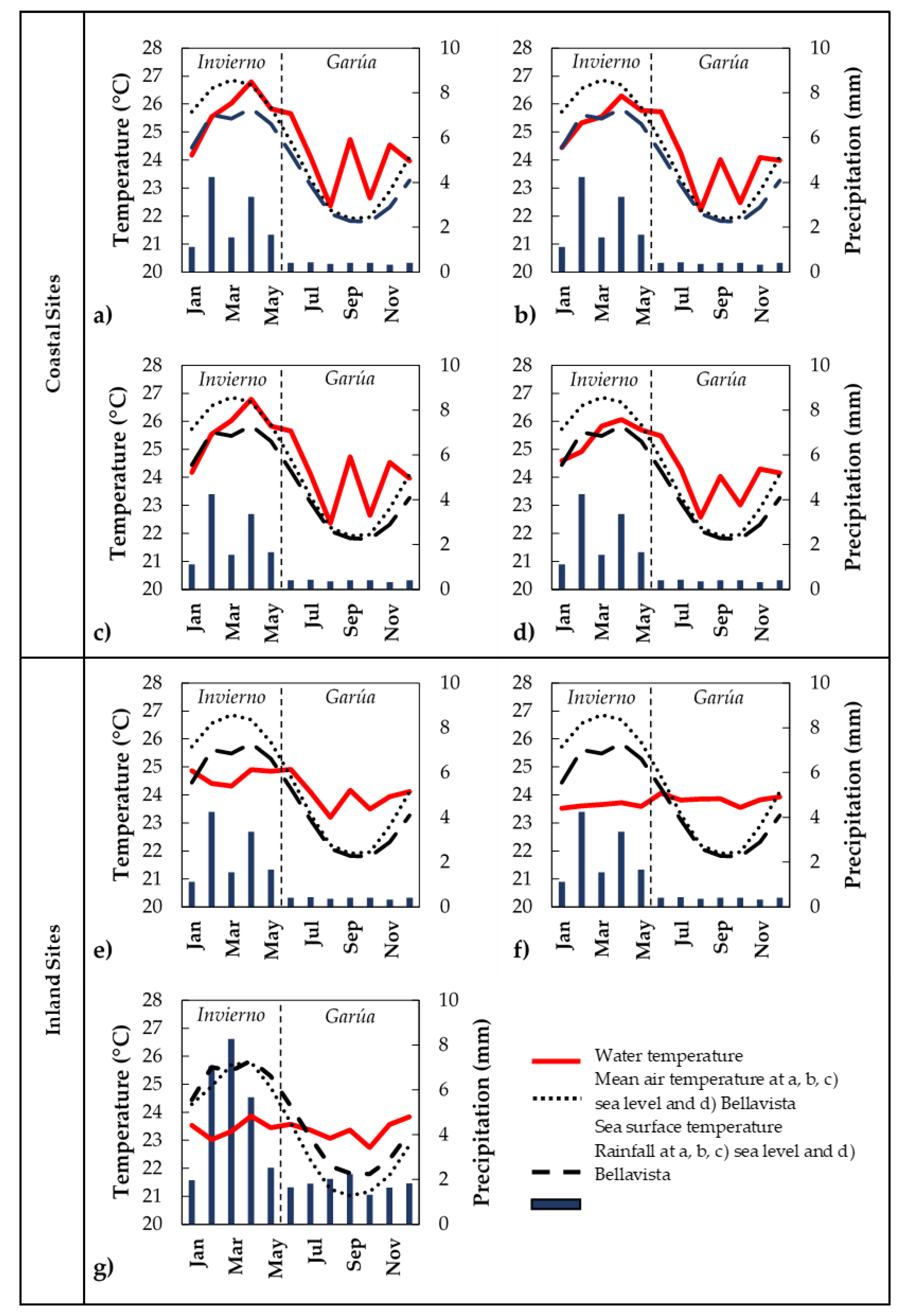
Climatic Conditions
2.2. Study Approach
2.2.1. Water Quality Parameters
2.2.2. Meteorological Variables
2.2.3. Evaluating Water Suitability for Designated Water Uses
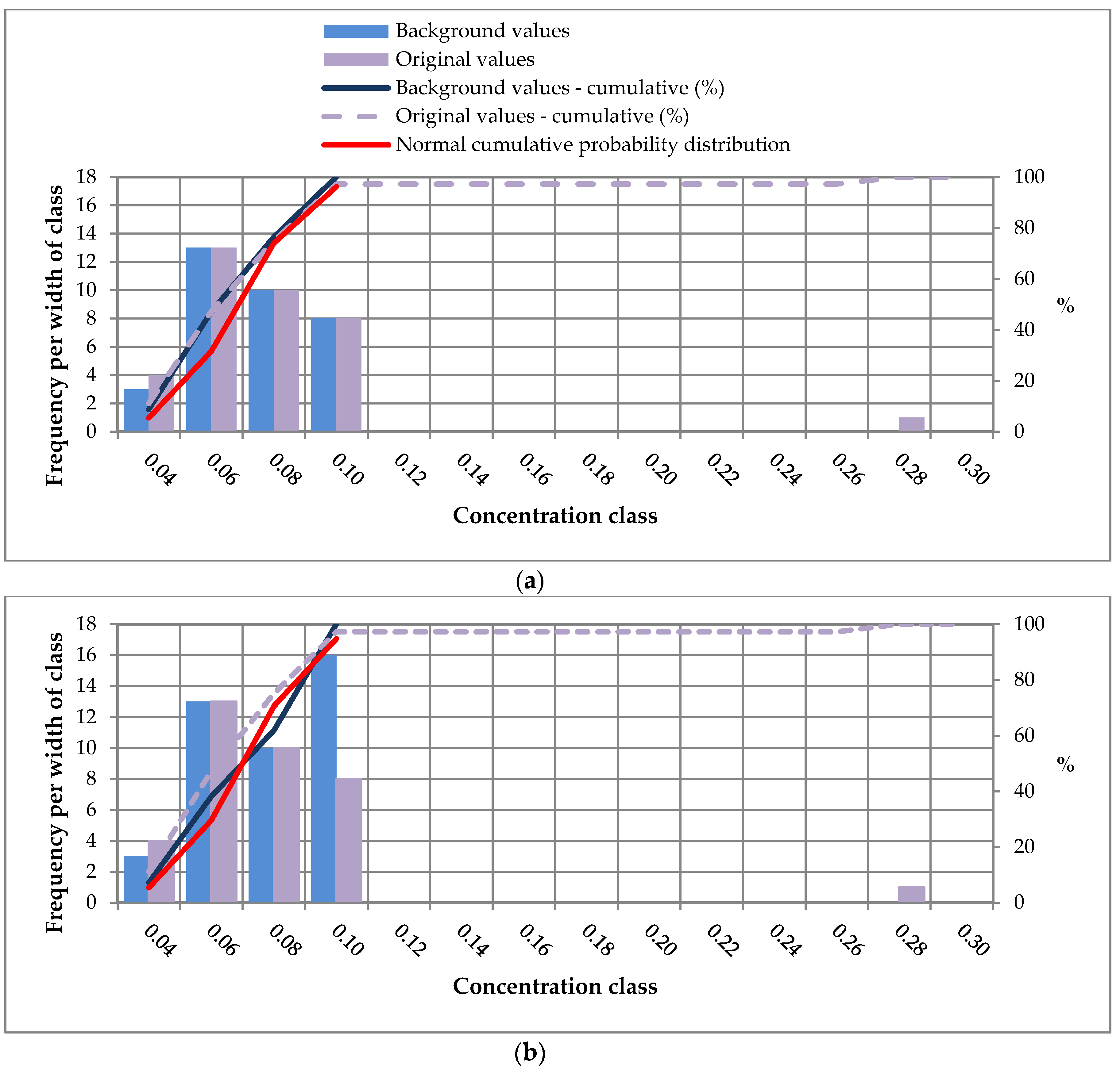
2.2.4. Statistical Techniques for Environmental Background Level Determination
2.2.5. Estimating Sensitivities to Changes Population
3. Results
3.1. Parameters Exceeding Water Quality Criteria and Guidelines
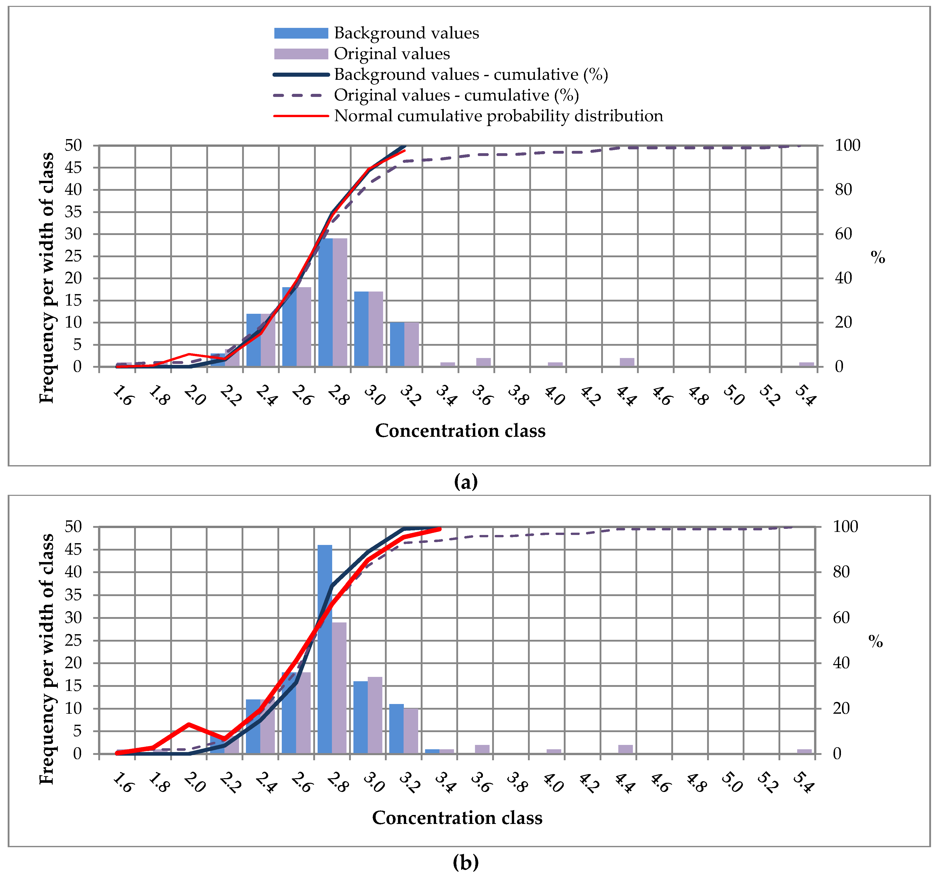
3.2. Environmental Background Levels
3.3. Relative Influence of Population Change on Water Quality Parameters
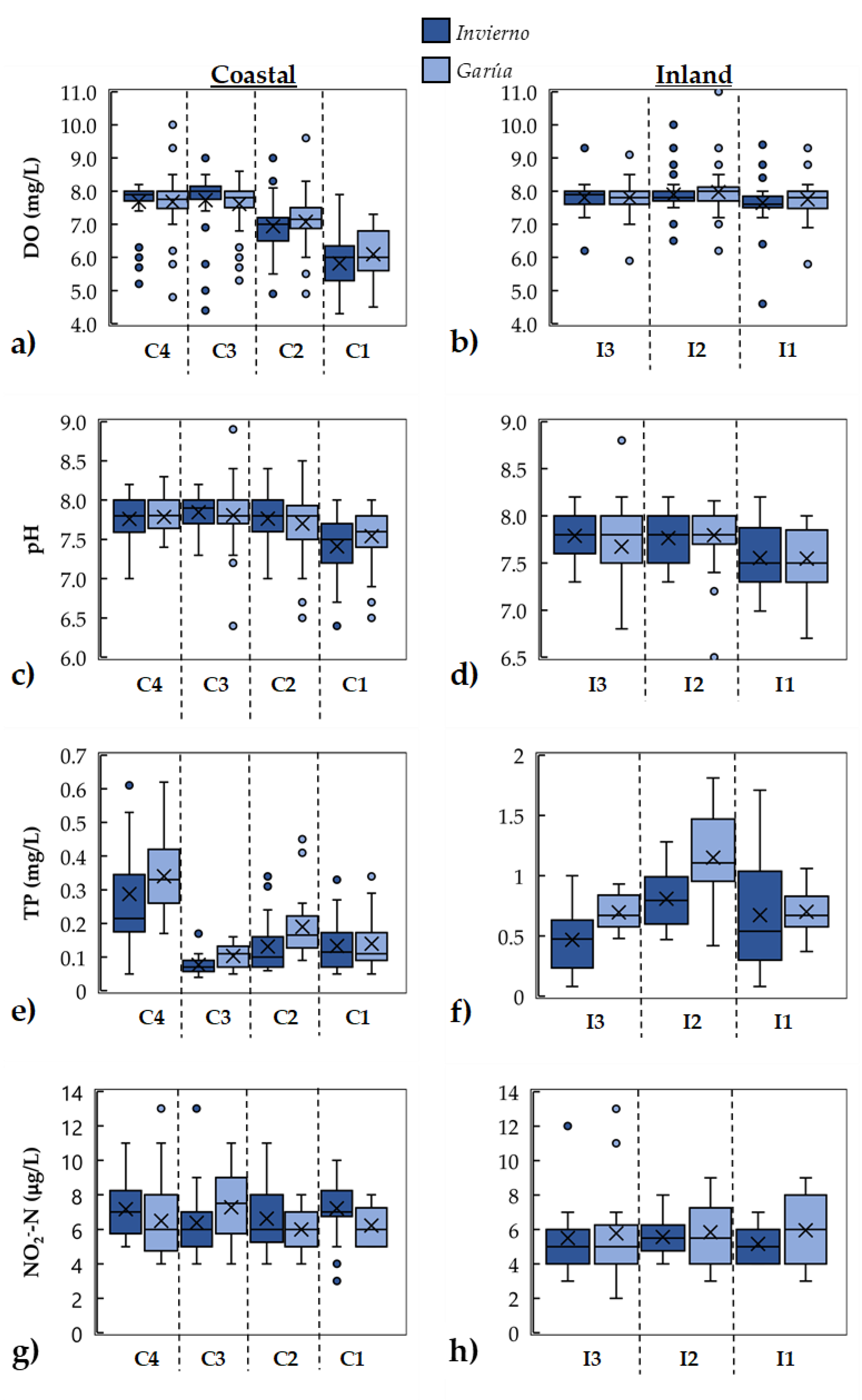
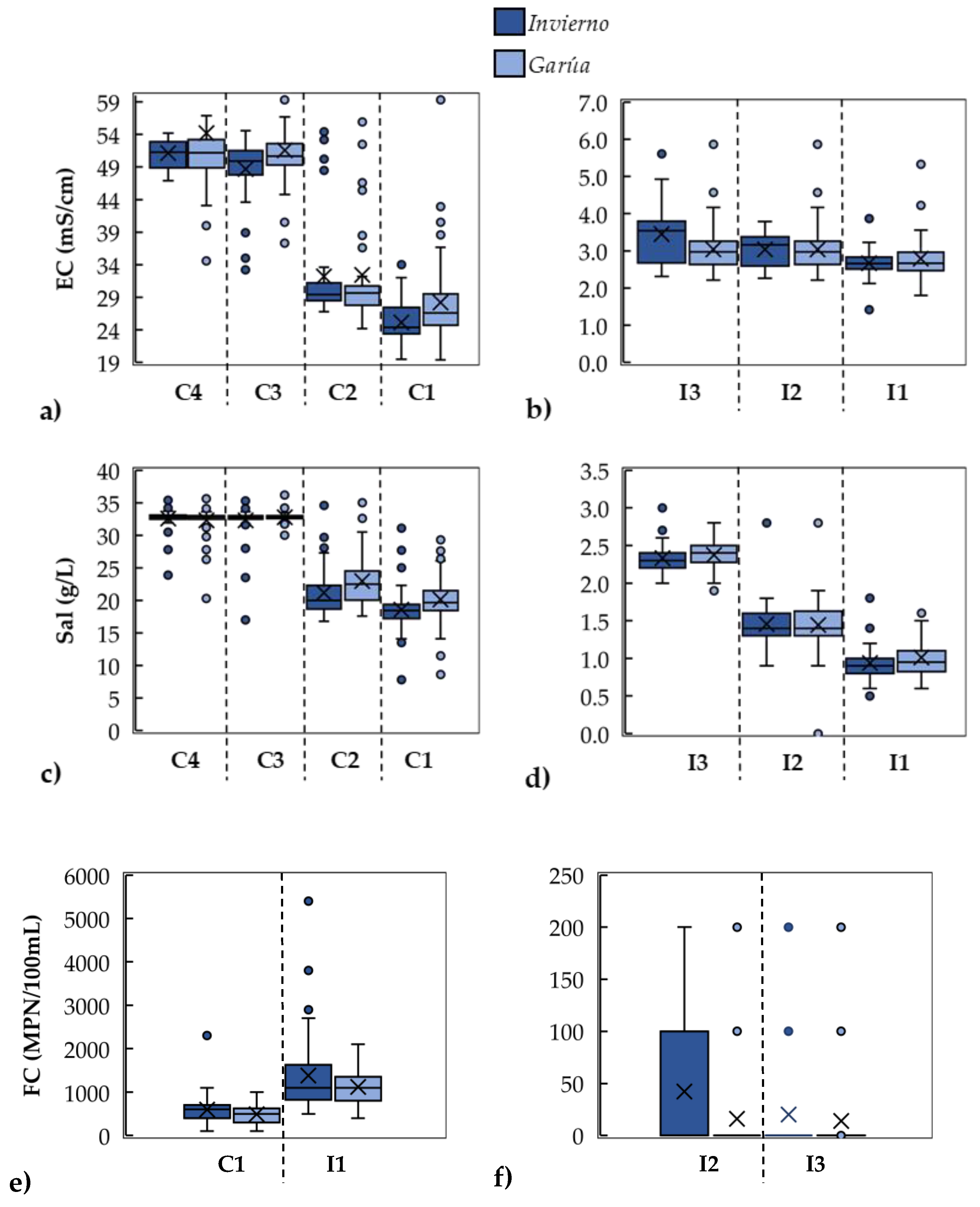
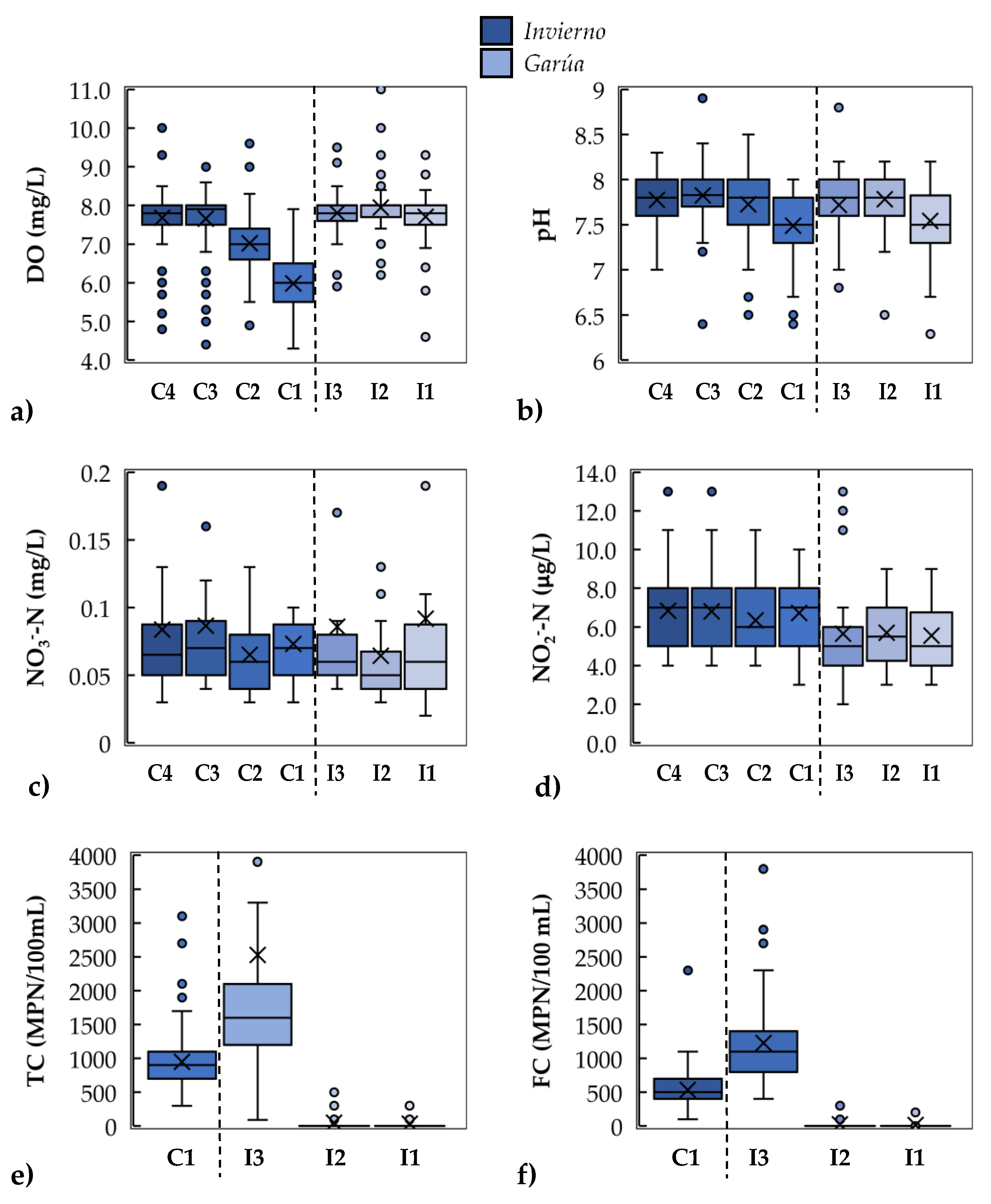
3.4. Seasonal Variations
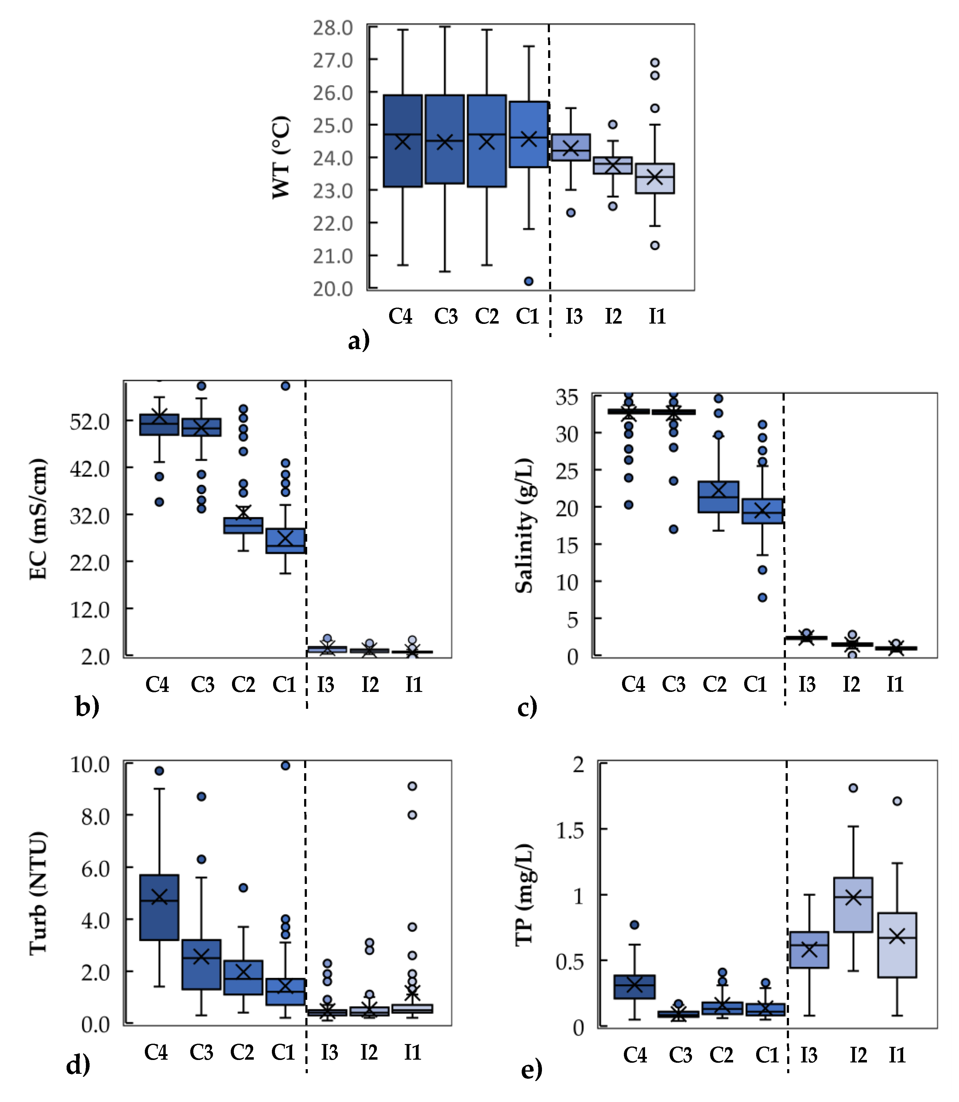
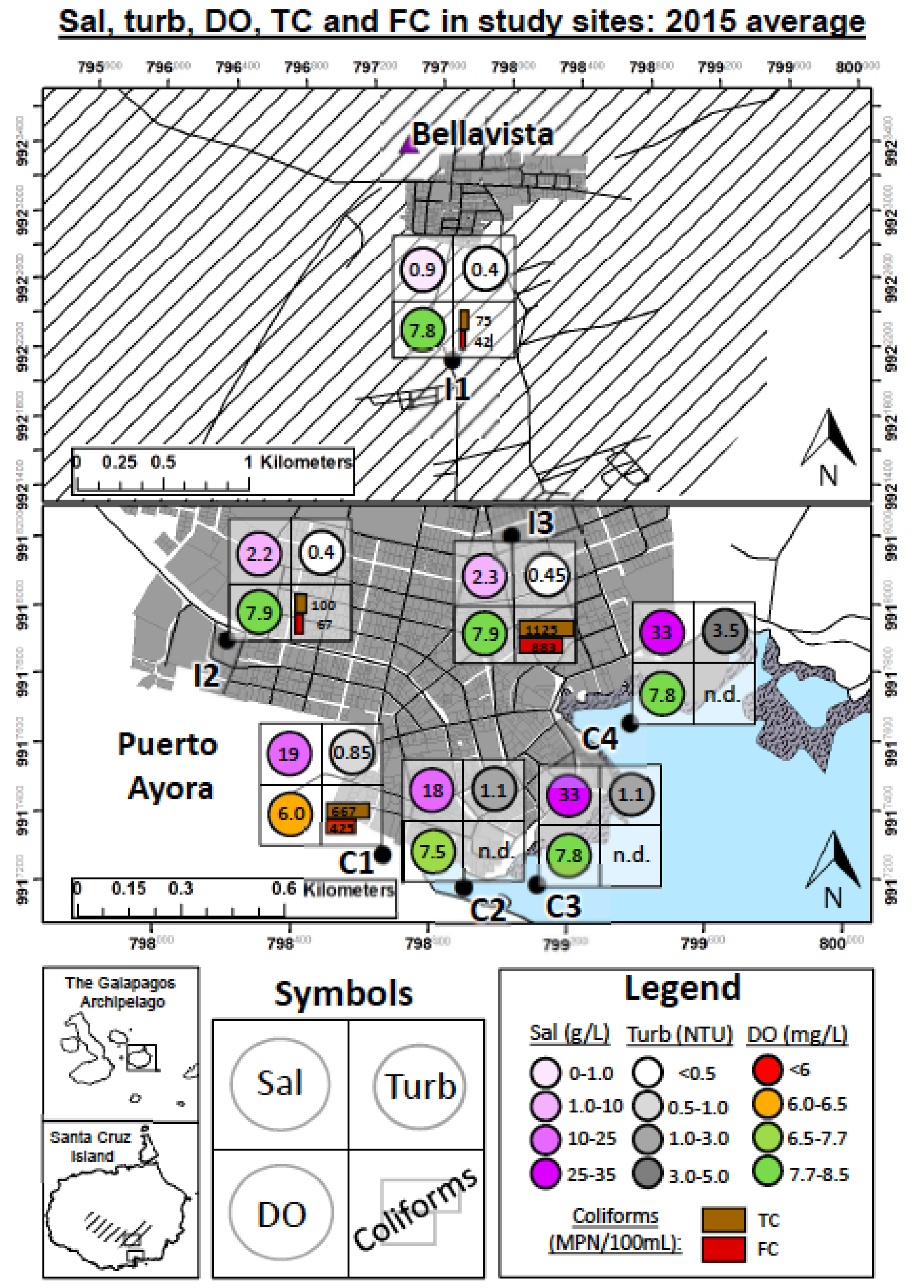
3.5. Spatial Variations
4. Discussion
4.1. Suitability Analysis for Drinking and Domestic Use
4.2. Suitability Analysis for Irrigation
4.3. Suitability Analysis for Wild and Aquatic Life in Coastal Waters and Estuaries
4.4. Environmental Background Levels
4.5. Relative Influence of Population Change on Water Quality Paramertes
5. Conclusions
Author Contributions
Funding
Acknowledgments
Conflicts of Interest
Appendix A

| Parameters | Abbreviations | Units | Time Coverage | ||||||
|---|---|---|---|---|---|---|---|---|---|
| I1 | I2 | I3 | C1 | C2 | C3 | C4 | |||
| Water temperature | WT | °C | ✓ | ✓ | ✓ | ✓ | ✓ | ✓ | ✓ |
| Turbidity | Turb | NTU | ✓ | ✓ | ✓ | ✓ | ✓ | ✓ | ✓ |
| Total Coliforms | TC | MPN 100 mL−1 | ✓ | ✓ | ✓ | ✓ | n.d. | n.d. | n.d. |
| Fecal Coliforms | FC | MPN 100 mL−1 | ✓ | ✓ | ✓ | ✓ | n.d. | n.d. | n.d. |
| Salinity | Sal | g L−1 | ✓ | ✓ | ✓ | ✓ | ✓ | ✓ | ✓ |
| Dissolved oxygen | DO | mg L−1 | ✓ | ✓ | ✓ | ✓ | ✓ | ✓ | ✓ |
| Electrical Conductivity | EC | mS cm−1 | ✓ | ✓ | ✓ | ✓ | ✓ | ✓ | ✓ |
| pH | pH | pH unit | ✓ | ✓ | ✓ | ✓ | ✓ | ✓ | ✓ |
| Nitrate | NO3−-N | mg L−1 | * | * | * | * | * | * | * |
| Nitrite | NO2−-N | μg L−1 | * | * | * | * | * | * | * |
| Total Phosphorus | TP | mg L−1 | * | * | * | * | * | * | * |


References
- Michalak, A.M. Study role of climate change in extreme threats to water quality. Nature 2016, 535, 349–350. [Google Scholar] [CrossRef]
- Whitehead, P.G.; Wilby, R.L.; Battarbee, R.W.; Kernan, M.; Wade, A.J. A review of the potential impacts of climate change on surface water quality. Hydrol. Sci. J. 2009, 54, 101–123. [Google Scholar] [CrossRef] [Green Version]
- Perkins, D.L.; Kann, J.; Scoppettone, G.G. The Role of Poor Water Quality and Fish Kills in the Decline of Endangered Lost River and Shortnose Suckers in Upper Klamath Lake; U.S. Geological Survey: Klamath Falls, OR, USA, 2000; p. 40. [Google Scholar]
- Liu, J.; d’Ozouville, N. Water Contamination in Puerto Ayora: Applied Interdisciplinary Research Using Escherichia Coli as an Indicator Bacteria; Galapagos Report 2011–2012; GNPD, GCREG, CDF and GC: Puerto Ayora, Galápagos, Ecuador, 2011; pp. 76–83. [Google Scholar]
- Walsh, S.J.; McCleary, A.L.; Heumann, B.W.; Brewington, L.; Raczkowski, E.J.; Mena, C.F. Community Expansion and Infrastructure Development: Implications for Human Health and Environmental Quality in the Galápagos Islands of Ecuador. J. Lat. Am. Geogr. 2010, 9, 137–159. [Google Scholar] [CrossRef]
- Overbey, K.N.; Hatcher, S.M.; Stewart, J.R. Water quality and antibiotic resistance at beaches of the Galápagos Islands. Front. Environ. Sci. 2015, 3. [Google Scholar] [CrossRef]
- Jun, X.; Shubo, C.; Xiuping, H.; Rui, X.; Xiaojie, L. Potential Impacts and Challenges of Climate Change on Water Quality and Ecosystem: Case Studies in Representative Rivers in China. J. Resour. Ecol. 2010, 1, 31–35. [Google Scholar]
- Kistemann, T.; Classen, T.; Koch, C.; Dangendorf, F.; Fischeder, R.; Gebel, J.; Vacata, V.; Exner, M. Microbial Load of Drinking Water Reservoir Tributaries during Extreme Rainfall and Runoff. Appl. Environ. Microbiol. 2002, 68, 2188–2197. [Google Scholar] [CrossRef] [Green Version]
- Pednekar, A.M.; Grant, S.B.; Jeong, Y.; Poon, Y.; Oancea, C. Influence of Climate Change, Tidal Mixing, and Watershed Urbanization on Historical Water Quality in Newport Bay, a Saltwater Wetland and Tidal Embayment in Southern California. Environ. Sci. Technol. 2005, 39, 9071–9082. [Google Scholar] [CrossRef] [PubMed]
- Delpla, I.; Jung, A.-V.; Baures, E.; Clement, M.; Thomas, O. Impacts of climate change on surface water quality in relation to drinking water production. Environ. Int. 2009, 35, 1225–1233. [Google Scholar] [CrossRef]
- Alava, J.J.; Palomera, C.; Bendell, L.; Ross, P.S. Pollution as an Emerging Threat for the Conservation of the Galapagos Marine Reserve: Environmental Impacts and Management Perspectives. In The Galapagos Marine Reserve; Denkinger, J., Vinueza, L., Eds.; Springer International Publishing: Cham, Switzerland, 2014; pp. 247–283. ISBN 978-3-319-02768-5. [Google Scholar]
- López, J.; Rueda, D. Water Quality Monitoring System in Santa Cruz, San Cristóbal, and Isabela; Galapagos Report 2009–2010; CDF, GNP & CGG: Puerto Ayora, Galapagos, Ecuador, 2010; pp. 103–107. [Google Scholar]
- CISPDR. Plan Reginal de los Recursos Hídricos de las Islas Galápagos; Changjiang Institute of Survey Planning Design and Research (CISPDR): London, UK, 2015. [Google Scholar]
- Violette, S.; d’Ozouville, N.; Pryet, A.; Deffontaines, B.; Fortin, J.; Adelinet, M. Hydrogeology of the Galápagos Archipelago: An Integrated and Comparative Approach Between Islands. Galápagos A Nat. Lab. Earth Sci. Geophys. Monogr. 2014, 204, 167–185. [Google Scholar]
- Palmer, M.; Armijos, E.; Moir, F.C. Selection of an ocean outfall site for the town of Puerto Ayora in the Galapagos Islands. In Proceedings of the XXVIII Congreso Interamericano de Ingeniería Sanitaria y Ambiental, Cancún, México, 27–31 October 2002. [Google Scholar]
- Malmaeus, J.M.; Blenckner, T.; Markensten, H.; Persson, I. Lake phosphorus dynamics and climate warming: A mechanistic model approach. Ecol. Model. 2006, 190, 1–14. [Google Scholar] [CrossRef]
- Sun, L.; Gui, H.; Peng, W. Geostatistical analyses of iron in shallow groundwater and their application for establishing an environmental baseline: A case study. Water Pract. Technol. 2014, 9, 450. [Google Scholar] [CrossRef]
- Gałuszka, A.; Migaszewski, Z.M.; Dołęgowska, S.; Michalik, A.; Duczmal-Czernikiewicz, A. Geochemical background of potentially toxic trace elements in soils of the historic copper mining area: A case study from Miedzianka Mt., Holy Cross Mountains, south-central Poland. Environ. Earth Sci. 2015, 74, 4589–4605. [Google Scholar] [CrossRef]
- Water Resources Glossaries. Available online: https://water.usgs.gov/water-basics_glossary.html#B (accessed on 7 April 2019).
- Nakić, Z.; Posavec, K.; Bačani, A. A Visual Basic Spreadsheet Macro for Geochemical Background Analysis. Ground Water 2007, 45, 642–647. [Google Scholar] [CrossRef] [PubMed]
- Urresti-Estala, B.; Carrasco-Cantos, F.; Vadillo-Pérez, I.; Jiménez-Gavilán, P. Determination of background levels on water quality of groundwater bodies: A methodological proposal applied to a Mediterranean River basin (Guadalhorce River, Málaga, southern Spain). J. Environ. Manag. 2013, 117, 121–130. [Google Scholar] [CrossRef] [PubMed]
- Zgłobicki, W.; Lata, L.; Plak, A.; Reszka, M. Geochemical and statistical approach to evaluate background concentrations of Cd, Cu, Pb and Zn (case study: Eastern Poland). Environ. Earth Sci. 2011, 62, 347–355. [Google Scholar] [CrossRef]
- d’Ozouville, N.; Deffontaines, B.; Benveniste, J.; Wegmüller, U.; Violette, S.; de Marsily, G. DEM generation using ASAR (ENVISAT) for addressing the lack of freshwater ecosystems management, Santa Cruz Island, Galapagos. Remote Sens. Environ. 2008, 112, 4131–4147. [Google Scholar] [CrossRef]
- d’Ozouville, N. Manejo de Recursos Hídricos: Caso de la Cuenca de Pelican Bay; Informe Galápagos 2007–2008; DPNG, CGREG, FCD y GC: Puerto Ayora, Ecuador, 2007. [Google Scholar]
- Pryet, A.; Domínguez, C.; Tomai, P.F.; Chaumont, C.; d’Ozouville, N.; Villacís, M.; Violette, S. Quantification of cloud water interception along the windward slope of Santa Cruz Island, Galapagos (Ecuador). Agric. For. Meteorol. 2012, 161, 94–106. [Google Scholar] [CrossRef] [Green Version]
- Stumpf, C.H.; González, R.A.; Noble, R.T. Chapter 10: Investigating the Coastal Water Quality of the Galapagos Islands, Ecuador. In Science and Conservation in the Galapagos Islands: Frameworks & Perspectives; Walsh, S.J., Mena, C.F., Eds.; Springer: New York, NY, USA, 2013; pp. 173–184. ISBN 2195-1055. [Google Scholar]
- Trueman, M.; d’Ozouville, N. Characterizing the Galapagos terrestrial climate in the face of global climate change. Galapagos Res. 2010, 67, 12. [Google Scholar]
- Adelinet, M.; Fortin, J.; d’Ozouville, N.; Violette, S. The relationship between hydrodynamic properties and weathering of soils derived from volcanic rocks, Galapagos Islands (Ecuador). Environ. Geol. 2008, 56, 45–58. [Google Scholar] [CrossRef]
- d’Ozouville, N. Etude du fonctionnement hydrologique dans les îles: Caractérisation d’un milieu volcani ue insulaire et préalable à la gestion de la ressource. Ph.D. Thesis, Université Pierre et Marie Curie, Paris, France, 2007. [Google Scholar]
- Zapata, F. Planificación del Monitoreo de la Contaminación Costera y Calidad del Agua en Puerto Ayora, Galápagos; Monitoreo de Ambientes Marinos; Parque Nacional Galápagos-JICA: Santa Cruz, CA, USA, 2004. [Google Scholar]
- Standard Methods for the Examination of Water and Wastewater, 22nd ed.; Rice, E.W.; American Public Health Association (Eds.) American Public Health Association: Washington, DC, USA, 2012; ISBN 978-0-87553-013-0. [Google Scholar]
- Snell, H.; Rea, S. The 1997–1998 El Niño in Galapagos: Can 34 years of data estimate 120 years of pattern. In Climate Change Vulnerability Assessment of the Galápagos Islands; Larrea Oña, I., Di Carlo, G., Eds.; WWF: Grand, Switzerland; Conservation International: Arlington, VA, USA, 2011; p. 10. ISBN 978-9942-03-454-0. [Google Scholar]
- MAE. Acuerdo 097-A, Anexo 1 del Libro VI del Texto Unificado de Legislación Secundaria del Ministerio del Ambiente: Norma de Calidad Ambiental y de Descarga de Efluentes al Recurso Agua; MAE: Quito, Ecuador, 2015. [Google Scholar]
- Guidelines for Drinking-Water Quality, 4th ed.; World Health Organization: Geneva, Switzerland, 2011.
- Water Quality Standards. In Hawaii Administrative Rules Title 11, Chapter 54—Water Quality Standards; 2015. Available online: epa.gov (accessed on 24 April 2019).
- MacDonald, G.; Abbott, A.; Peterson, F.L. Volcanoes in the Sea; The Geology of Hawaii; University of Hawaii Press: Honolulu, HI, USA, 1983; p. 517. [Google Scholar]
- Benson, B.B.; Krause, D. The Concentration and Isotopic Fractionation of Gases Dissolved in Freshwater in Equilibrium with the Atmosphere. 1. Oxygen. Limnol. Oceanogr. 1984, 25, 662–671. [Google Scholar] [CrossRef]
- Matschullat, J.; Ottenstein, R.; Reimann, C. Geochemical background—Can we calculate it? Environ. Geol. 2000, 39, 990–1000. [Google Scholar] [CrossRef]
- Bu, H.; Meng, W.; Zhang, Y.; Wan, J. Relationships between land use patterns and water quality in the Taizi River basin, China. Ecol. Indic. 2014, 41, 187–197. [Google Scholar] [CrossRef]
- Shi, W.; Xia, J.; Zhang, X. Influences of anthropogenic activities and topography on water quality in the highly regulated Huai River basin, China. Environ. Sci. Pollut. Res. 2016, 23, 21460–21474. [Google Scholar] [CrossRef] [PubMed]
- Halstead, J.A.; Kliman, S.; Berheide, C.W.; Chaucer, A.; Cock-Esteb, A. Urban stream syndrome in a small, lightly developed watershed: A statistical analysis of water chemistry parameters, land use patterns, and natural sources. Environ. Monit. Assess. 2014, 186, 3391–3414. [Google Scholar] [CrossRef] [PubMed]
- Ahamad, K.U.; Raj, P.; Barbhuiya, N.H.; Deep, A. Surface Water Quality Modeling by Regression Analysis and Artificial Neural Network. In Advances in Waste Management; Kalamdhad, A., Singh, J., Dhamodharan, K., Eds.; Springer: Singapore, 2019; pp. 215–230. [Google Scholar]
- Tasker, G.D.; Driver, N.E. Nationwide Regression Models for Predicting Urban Runoff Water Quality at Unmonitored Sites. JAWRA J. Am. Water Res. Assoc. 1988, 24, 1091–1101. [Google Scholar] [CrossRef]
- Christensen, V.; Xiaodong, J.; Ziegler, A. Regression Analysis and Real-Time Water-Quality Monitoring to Estimate Constituent Concentrations, Loads, and Yields in the Little Arkansas River, South-Central Kansas, 1995–1999; U.S. Geological Survey & U.S. Department of Interior: Washington, DC, USA, 2000. [Google Scholar]
- Instituto Nacional de Estatisticas y Censos (INEC). Censo de Población Y Vivienda 2011: Quito, Ecuador. Proyección a 2018. Available online: http://www.ecuadorencifras.gob.ec/ (accessed on 8 July 2018).
- Ministerio de Turismo Observatorio de Turismo de Galápagos. Available online: https://www.observatoriogalapagos.gob.ec/ (accessed on 1 April 2019).
- Kovač, Z.; Nakić, Z.; Pavlić, K. Influence of groundwater quality indicators on nitrate concentrations in the Zagreb aquifer system. Geol. Croat. 2017, 70, 93–103. [Google Scholar] [CrossRef]
- New Zealand’s Environmental Reporting Series: Environment Aotearoa 2015; Ministry for the Environment & Statistics New Zealand: Wellington, New Zealand, 2015.
- Kaplan, D.M.; Largier, J.L.; Navarrete, S.; Guiñez, R.; Castilla, J.C. Large diurnal temperature fluctuations in the nearshore water column. Estuar. Coast. Shelf Sci. 2003, 57, 385–398. [Google Scholar] [CrossRef]
- Kurylyk, B.L.; Bourque, C.P.-A.; MacQuarrie, K.T.B. Potential surface temperature and shallow groundwater temperature response to climate change: An example from a small forested catchment in east-central New Brunswick (Canada). Hydrol. Earth Syst. Sci. 2013, 17, 2701–2716. [Google Scholar] [CrossRef]
- Szczucińska, A.M.; Wasielewski, H. Seasonal Water Temperature Variability of Springs from Porous Sediments in Gryżynka Valley, Western Poland. Quaest. Geogr. 2013, 32. [Google Scholar] [CrossRef]
- Howarth, R.W.; Sharpley, A.; Walker, D. Sources of nutrient pollution to coastal waters in the United States: Implications for achieving coastal water quality goals. Estuaries 2002, 25, 656–676. [Google Scholar] [CrossRef]
- Werner, A.D.; Bakker, M.; Post, V.E.A.; Vandenbohede, A.; Lu, C.; Ataie-Ashtiani, B.; Simmons, C.T.; Barry, D.A. Seawater intrusion processes, investigation and management: Recent advances and future challenges. Adv. Water Res. 2013, 51, 3–26. [Google Scholar] [CrossRef] [Green Version]
- Molinari, A.; Chidichimo, F.; Straface, S.; Guadagnini, A. Assessment of natural background levels in potentially contaminated coastal aquifers. Sci. Total Environ. 2014, 476–477, 38–48. [Google Scholar] [CrossRef]
- Wang, Q.; Huo, Z.; Zhang, L.; Wang, J.; Zhao, Y. Impact of saline water irrigation on water use efficiency and soil salt accumulation for spring maize in arid regions of China. Agric. Water Manag. 2016, 163, 125–138. [Google Scholar] [CrossRef]
- Diaz, R.J.; Rosenberg, R. Marine benthic hypoxia: A review of its ecological effects and the behavioral responses of benthic macrofauna. Oceanogr. Morine Biol. An Annu. Rev. 1995, 33, 245–303. [Google Scholar]
- Parameters of Water Quality: Interpretation and Standards; Environmental Protection Agency: Dublin, Ireland, 2001; p. 133.
- Colford, J.M.; Wade, T.J.; Schiff, K.C.; Wright, C.C.; Griffith, J.F.; Sandhu, S.K.; Burns, S.; Sobsey, M.; Lovelace, G.; Weisberg, S.B. Water Quality Indicators and the Risk of Illness at Beaches with Nonpoint Sources of Fecal Contamination. Epidemiology 2007, 18, 27–35. [Google Scholar] [CrossRef] [PubMed]
- Werdeman, J. Effects of Populated Towns on Water Quality in Neighboring Galapagos Bays. Available online: http://courses.washington.edu/ocean443/2005_6/DraftProposals/Joni.pdf (accessed on 24 April 2019).
- Yang, X.; Liu, Q.; Luo, X.; Zheng, Z. Spatial Regression and Prediction of Water Quality in a Watershed with Complex Pollution Sources. Sci. Rep. 2017, 7. [Google Scholar] [CrossRef] [PubMed]


| Parameters | Guideline/Criteria Values | % of Exceedance | |||||
| I1 | I2 | I3 | |||||
| (A) Drinking and domestic use | |||||||
| FC a | 1000 MPN/100 mL | - | - | 53 | |||
| pH a | 6–9 | - | - | 2 | |||
| Sal b | Unpalatable: >1 g/L | 26 | 90 | 100 | |||
| Turb b | <1 NTU | 18 | 6 | 4 | |||
| (B) Irrigation water c | |||||||
| pH | 6–9 | - | - | 2 | |||
| FC | 1000 MPN/100 mL | - | - | 53 | |||
| EC | Moderate: 0.7–3 mS/cm | 83 | 51 | 33 | |||
| Severe: >3 mS/cm | 17 | 49 | 67 | ||||
| Sal | Moderate: 0.45–2 g/L | 99 | 76 | 6 | |||
| Severe: >2 g/L | 0 | 24 | 94 | ||||
| Parameters | Guideline/Criteria Values | % of Exceedance | |||||
| C1 | C2 | C3 | C4 | ||||
| (A) Preservation of wild and aquatic life in marine waters and estuaries d | |||||||
| DO | >60% saturation | 15 | 3 | 3 | 1 | ||
| pH | 6.5–9.5 | 2 | - | 1 | 1 | ||
| Turb | Shall not deviate more than 5% from background levels | 4 | 16 | 7 | 14 | ||
| (B) Primary and Secondary contact recreational water e | |||||||
| FC | 200 MPN/100 mL | 88 | n.d. | n.d. | n.d. | ||
| TC | 2000 MPN/100 mL | 4 | n.d. | n.d. | n.d. | ||
| DO | >80% saturation | 77 | 27 | 15 | 8 | ||
| pH | 6.5–8.3 (primary) | 3 | 2 | 3 | 1 | ||
| 6–9 (secondary) | 2 | - | - | 1 | |||
| (C) Specific criteria for estuaries and embayment f | |||||||
| [NO3−+NO2−]-N | 25 μg/L (estuaries) | 100 | 100 | 99 | - | ||
| 20 μg/L (embayments) | - | - | - | 99 | |||
| TP | 50 μg/L | 97 | 100 | 86 | 99 | ||
| Turb | 3 NTU | 8 | 20 | 40 | 99 | ||
| pH | 7-8.6 and shall not deviate more than 0.5 units from background levels | 10 | - | - | - | ||
| shall not deviate more than 0.5 units from 8.1 | - | 32 | 20 | 18 | |||
| DO | >75% sat. | 69 | 14 | 10 | 6 | ||
| WT | shall not deviate more than 1 °C from background levels | 5 | 2 | 1 | 1 | ||
| Sal | shall not deviate more than 10% C from background levels | 13 | 15 | 9 | 9 | ||
| (a) Inland Sites | ||||||||||
| Parameters | I1 | I2 | I3 | |||||||
| 2σ | d.f. | 2σ | d.f. | 2σ | d.f. | |||||
| WT (°C) | 22.4–24.3 | 18.8–28.0 | 23.4–24.2 | 23.0–24.6 | 23.8–24.4 | 22.9–25.5 | ||||
| Turb (NTU) | 0.2–0.7 | 0.2–0.8 | 0.1–0.6 * | 0.1–0.6 | 0.1–0.6 * | 0.1–0.7 * | ||||
| Sal (g/L) | 0.7–1.2 * | 0.7–1.1 | 1.1–1.8 | 0.8–2.0 | 2.1–2.6 | 2.0–2.6 | ||||
| DO (mg/L) | 7.2–8.3 | 6.6–9.0 | 7.6–8.3 | 7.2–8.8 | 7.6–8.3 * | 7.2–8.8 | ||||
| EC (mS/cm) | 2.1–3.2 * | 2.0–3.3 | 2.2–3.7 * | 2.2–3.7 * | 2.0–4.7 * | 1.9–5.1 * | ||||
| pH | 7.0–8.3 | 6.8–8.6 * | 7.4–8.2 | 7.2–8.4 | 7.5–8.2 | 7.5–8.2 * | ||||
| NO3−-N (mg/L) | 0.0–0.1 * | 0.0–0.1 * | 0.0–0.1 * | 0.0–0.1 * | 0.1–0.4 * | 0.1–0.4 * | ||||
| NO2−-N (μg/L) | 2.6–8.1 | 3.2–6.8 | 2.6–8.0 | 2.9–7.1 | 2.9–7.4 * | 2.7–7.3 | ||||
| TP (mg/L) | 0.0–1.3 * | 0.0–1.4 * | 0.0–1.6 * | 0.0–1.7 * | 0.0–1.1 * | 0.0–1.3 * | ||||
| (b) Coastal Sites | ||||||||||
| Parameters | C1 | C2 | C3 | C4 | ||||||
| 2σ | d.f. | 2σ | d.f. | 2σ | d.f. | 2σ | d.f. | |||
| WT (°C) | 23.1–26.5 | 21.7–27.7 | 21.8–27.2 * | 21.5–27.9 * | 21.7–27.3 * | 21.3–27.9 * | 21.9–27.6 * | 21.3–28.3 * | ||
| Turb (NTU) | 0.0–2.3 * | 0.1–2.3 * | 0.3–2.9 * | 0.4–3.2 * | 0.0–4.7 | 0.0–5.2 | 1.2–7.5 * | 1.2–8.4 * | ||
| Sal (g/L) | 16.4–21.6 * | 13.3–25.1 | 16.8–24.1 * | 16.7–25.9 * | 32.4–33.2 * | 28.0–37.6 | 32.4–33.2 * | 28.0–37.6 | ||
| DO (mg/L) | 4.7–7.4 | 4.5–7.9 | 6.5–7.8 | 5.5–8.5 | 7.5–8.3 | 7.5–8.3 * | 7.5–8.2 | 6.1–9.5 | ||
| EC (mS/cm) | 21.0–29.4 * | 20.2–30.3 | 26.4–31.7 * | 25.6–33.5 * | 47.1–53.9 * | 39.5–61.1 | 46.8–55.0 * | 39.5–61.1 | ||
| pH | 7.0–8.1 * | 6.4–8.6 | 7.4–8.2 | 7.1–8.5 | 7.5–8.2 * | 7.2–8.4 | 7.5–8.2 | 7.1–8.5 | ||
| NO3−-N (mg/L) | 0.0–0.1 | 0.0–0.1 * | 0.0–0.1 | 0.0–0.1 * | 0.0–0.1 * | 0.0–0.1 * | 0.0–0.1 * | 0.0–0.1 * | ||
| NO2−-N (μg/L) | 3.9–9.1 * | 3.7–10.3 * | 3.5–8.8 * | 3.9–8.1 * | 3.3–9.5 * | 3.4–10.6 * | 3.4–10.0 * | 3.7–10.3 * | ||
| TP (mg/L) | 0.0–0.2 * | 0.0–0.2 * | 0.0–0.2 * | 0.0–0.3 * | 0.0–0.5 * | 0.0–0.6 * | 0.0–0.5 * | 0.0–0.6 * | ||
| Inland Sites | Coastal Sites | ||||||||
|---|---|---|---|---|---|---|---|---|---|
| Site | Parameter | ß1 | ßo | R2 | Site | Parameter | ß1 | ßo | R2 |
| I1 | TEMP | −0.92 | 0.04 | 0.29 | C1 | TEMP | 0.14 | 0.03 | 0.01 |
| EC | 0.10 | 0.03 | 0.16 | EC | 0.05 | 0.03 | 0.07 | ||
| PH | 0.20 | 0.03 | 0.02 | PH | 0.58 | 0.03 | 0.58 | ||
| TURB | 0.00 | 0.32 | 0.00 | TURB | 0.02 | 0.03 | 0.19 | ||
| SAL | 0.07 | 0.04 | 0.06 | SAL | 0.19 | 0.03 | 0.24 | ||
| DO | −0.47 | 0.04 | 0.25 | DO | 0.10 | 0.03 | 0.13 | ||
| NO2-N | 0.02 | 0.03 | 0.00 | NO2-N | 0.10 | 0.04 | 0.17 | ||
| NO3-N | −0.01 | 0.03 | 0.01 | NO3-N | 0.00 | 0.03 | 0.00 | ||
| TP | −0.03 | 0.02 | 0.07 | TP | 0.01 | 0.03 | 0.00 | ||
| TC | 0.00 | 0.03 | 0.03 | TC | 0.01 | 0.03 | 0.03 | ||
| FC | 0.00 | 0.03 | 0.03 | FC | 0.06 | 0.03 | 0.29 | ||
| I2 | TEMP | 0.04 | 0.03 | 0.00 | C2 | TEMP | 0.08 | 0.03 | 0.00 |
| EC | 0.15 | 0.04 | 0.30 | EC | 0.19 | 0.04 | 0.72 | ||
| PH | 0.70 | 0.03 | 0.21 | PH | 0.84 | 0.03 | 0.43 | ||
| TURB | 0.36 | 0.03 | 0.14 | TURB | 0.08 | 0.04 | 0.38 | ||
| SAL | 0.00 | 0.03 | 0.00 | SAL | 0.09 | 0.03 | 0.05 | ||
| DO | 0.87 | 0.04 | 0.47 | DO | 0.20 | 0.03 | 0.46 | ||
| NO2-N | 0.01 | 0.03 | 0.01 | NO2-N | 0.08 | 0.03 | 0.08 | ||
| NO3-N | 0.01 | 0.03 | 0.00 | NO3-N | 0.04 | 0.03 | 0.38 | ||
| TP | 0.02 | 0.03 | 0.02 | TP | 0.02 | 0.04 | 0.72 | ||
| TC | 0.01 | 0.03 | 0.04 | TC | NA | NA | NA | ||
| FC | 0.00 | 0.32 | 0.00 | FC | NA | NA | NA | ||
| I3 | TEMP | 0.60 | 0.03 | 0.02 | C3 | TEMP | 0.28 | 0.03 | 0.09 |
| EC | 0.09 | 0.04 | 0.11 | EC | 0.02 | 0.03 | 0.10 | ||
| PH | 0.45 | 0.03 | 0.03 | PH | 1.58 | 0.03 | 0.21 | ||
| TURB | 0.04 | 0.04 | 0.30 | TURB | 0.03 | 0.03 | 0.02 | ||
| SAL | 0.11 | 0.03 | 0.09 | SAL | 3.28 | 0.04 | 0.79 | ||
| DO | 0.42 | 0.03 | 0.04 | DO | 0.23 | 0.04 | 0.22 | ||
| NO2-N | 0.09 | 0.03 | 0.12 | NO2-N | 0.05 | 0.03 | 0.30 | ||
| NO3-N | 0.02 | 0.03 | 0.29 | NO3-N | 0.07 | 0.04 | 0.52 | ||
| TP | 0.17 | 0.04 | 0.26 | TP | 0.08 | 0.03 | 0.42 | ||
| TC | 0.05 | 0.04 | 0.21 | TC | NA | NA | NA | ||
| FC | 0.10 | 0.04 | 0.34 | FC | NA | NA | NA | ||
| C4 | TEMP | 0.35 | 0.04 | 0.14 | |||||
| EC | 0.02 | 0.03 | 0.09 | ||||||
| PH | 0.57 | 0.03 | 0.15 | ||||||
| TURB | 0.16 | 0.05 | 0.46 | ||||||
| SAL | 0.47 | 0.03 | 0.05 | ||||||
| DO | 0.50 | 0.04 | 0.22 | ||||||
| NO2-N | 0.04 | 0.03 | 0.13 | ||||||
| NO3-N | 0.08 | 0.04 | 0.49 | ||||||
| TP | 0.02 | 0.03 | 0.02 | ||||||
| TC | NA | NA | NA | ||||||
| FC | NA | NA | NA | ||||||
© 2019 by the authors. Licensee MDPI, Basel, Switzerland. This article is an open access article distributed under the terms and conditions of the Creative Commons Attribution (CC BY) license (http://creativecommons.org/licenses/by/4.0/).
Share and Cite
Mateus, C.; Guerrero, C.A.; Quezada, G.; Lara, D.; Ochoa-Herrera, V. An Integrated Approach for Evaluating Water Quality between 2007–2015 in Santa Cruz Island in the Galapagos Archipelago. Water 2019, 11, 937. https://doi.org/10.3390/w11050937
Mateus C, Guerrero CA, Quezada G, Lara D, Ochoa-Herrera V. An Integrated Approach for Evaluating Water Quality between 2007–2015 in Santa Cruz Island in the Galapagos Archipelago. Water. 2019; 11(5):937. https://doi.org/10.3390/w11050937
Chicago/Turabian StyleMateus, Cristina, Christian A. Guerrero, Galo Quezada, Daniel Lara, and Valeria Ochoa-Herrera. 2019. "An Integrated Approach for Evaluating Water Quality between 2007–2015 in Santa Cruz Island in the Galapagos Archipelago" Water 11, no. 5: 937. https://doi.org/10.3390/w11050937