On the Predictability of Daily Rainfall during Rainy Season over the Huaihe River Basin
by
 , ,
, ,
Qing Cao
1,2, 
Zhenchun Hao
1,2,3,*,
Feifei Yuan
1,2,*,
Ronny Berndtsson
4,
Shijie Xu
1,2,
Huibin Gao
1,2 and
Jie Hao
5 1
State Key Laboratory of Hydrology Water Resources and Hydraulic Engineering, Hohai University, Nanjing 210098, China
2
Department of hydrology and water resources, Hohai University, Nanjing 210098, China
3
National Cooperative Innovation Center for Water Safety & Hydro-Science, Hohai University, Nanjing 210098, China
4
Department of Water Resources Engineering and Center for Middle Eastern Studies, Lund University, P.O. Box 118, SE-221 00 Lund, Sweden
5
Nanjing Hydraulic Research Institute, Nanjing 210098, China
*
Authors to whom correspondence should be addressed.
Water 2019, 11(5), 916; https://doi.org/10.3390/w11050916
Submission received: 10 April 2019
/
Revised: 26 April 2019
/
Accepted: 29 April 2019
/
Published: 1 May 2019
(This article belongs to the Section Hydrology)
Abstract
:In terms of climate change and precipitation, there is large interest in how large-scale climatic features affect regional rainfall amount and rainfall occurrence. Large-scale climate elements need to be downscaled to the regional level for hydrologic applications. Here, a new Nonhomogeneous Hidden Markov Model (NHMM) called the Bayesian-NHMM is presented for downscaling and predicting of multisite daily rainfall during rainy season over the Huaihe River Basin (HRB). The Bayesian-NHMM provides a Bayesian method for parameters estimation. The model avoids the risk to have no solutions for parameter estimation, which often occurs in the traditional NHMM that uses point estimates of parameters. The Bayesian-NHMM accurately captures seasonality and interannual variability of rainfall amount and wet days during the rainy season. The model establishes a link between large-scale meteorological characteristics and local precipitation patterns. It also provides a more stable and efficient method to estimate parameters in the model. These results suggest that prediction of daily precipitation could be improved by the suggested new Bayesian-NHMM method, which can be helpful for water resources management and research on climate change.
1. Introduction
Precipitation simulation in time and space plays a significant role in management of the physical environment of humans and is important to mitigate disasters such as floods. Climatic fluctuation is a major driver of precipitation amount [1]. Statistical downscaling (SD) is a class of methods used to model the effects of large-scale climate variation on daily precipitation. Thus, SD is important for the understanding of cross-scale linkages in order to better visualize the physical relations between large and small atmospheric scales.
A wide range of SD models have been developed during the last 20 years [2,3,4]. A detailed comparison among different SD models in terms of predictors, skill measures, and working principles has been performed by several previous researchers [5,6,7,8,9]. An example of SD models is the Homogeneous and Nonhomogeneous Hidden Markov Models (HMM vs. NHMM), which are efficient in capturing the most distinct patterns affecting multisite rainfall occurrence and amount.
The HMM and NHMM have been used worldwide for statistical downscaling of daily rainfall and in research on climate change [10,11,12,13,14,15,16]. The HMM is a state-based model in which each day is related to a particular hidden state, which follows a first-order Markov chain. Thus, HMM can translate a sequence of observations (precipitation amount and occurrence) into a stochastic process. In the HMM, changes among states are controlled by a transition matrix, which only depends on the current state. In the NHMM, the transition matrix is influenced not only by the current hidden state but also on atmospheric variables. This feature enables the NHMM to demonstrate both spatial covariance and temporal dependence between precipitation and climatic variables over the network. The Expectation-Maximization (EM) algorithm is usually used for parameter estimation in the NHMM. However, the EM algorithm relies on point estimates of parameters and has no solutions for complex spatial situations [1,14].
Greene et al. [17] introduced a new NHMM (Bayesian-NHMM) to solve this problem where the Bayesian method is used to estimate parameters. The Bayesian framework can provide uncertainty estimates for all parameters in the model, which allows for an automatic assessment of the effect of each exogenous atmospheric variable. This approach is better suited to feature uncertainty in parameter estimation as compared to the EM approach. In addition, exogenous variables introduced in the traditional NHMM as predictors are only large-scale climate data, which only influence the transition probabilities. In the Bayesian-NHMM, there are two types of exogenous variables (large-scale and region-scale variables). Predictors at the regional scale are used to affect the occurrence distribution of precipitation and can provide more local rainfall information in the model. As a consequence, the Bayesian-NHMM enables new analyses of precipitation variability integrated from local-to-subcontinental spatial scales, which can generate chains with different levels of exogenous variables.
There have been some applications of the Bayesian-NHMM to simulate daily precipitation. Greene et al. [17] used the Bayesian-NHMM to simulate rainfall features in the region of the Indo-Gangetic plain. They pointed out that the model can well capture rainfall characteristics at different rainfall stations. Holsclaw et al. [18] modeled daily precipitation using Bayesian-NHMM over the Yangtze River Basin in China and argued that the model can efficiently represent summer rainfall in terms of seasonality and interannual variability. Holsclaw et al. [19] applied the Bayesian-NHMM to downscale daily rainfall in India. They concluded that the model can capture temporal and spatial rainfall features. However, application of the Bayesian-NHMM over the Huaihe River Basin (HRB) has not yet been performed. The HRB is an important grain-producing area, which makes up for approximately 20% of the total grain production in China [20,21,22]. The HRB, however, is prone to flood and drought, due to the fact that precipitation in this area varies greatly both inter-seasonally and inter-annually. More than 60 floods and 40 droughts during the period 1470–2018 have occurred in the HRB, where recurrent frequency is typically four years [23,24]. More than half of the annual precipitation concentrates to the rainy season. However, simulation of precipitation during the rainy season and the influence of large-scale atmospheric mechanisms on rainy-season precipitation in the HRB are still not well understood.
Motivated by the need for improved understanding of rainy-season precipitation in the HRB, this study aims at using the Bayesian-NHMM in terms of analysis of its ability to capture seasonality of precipitation during the rainy season. The ability to represent interannual variability of daily precipitation amount and wet days during rainy season will also be tested. This work can, thus, contribute to the development of a new NHMM method to predict daily rainfall under climate shift.
The remainder of the study is organized as follows: Section 2 describes the HRB and data, and Section 3 introduces methods used in this study (e.g., determination of rainy season and the Bayesian-NHMM). Section 4 analyzes hidden rainfall states and examines rainfall simulations by the model. Finally, a conclusion is presented in Section 5.
2. Study Area and Data
2.1. Study Area
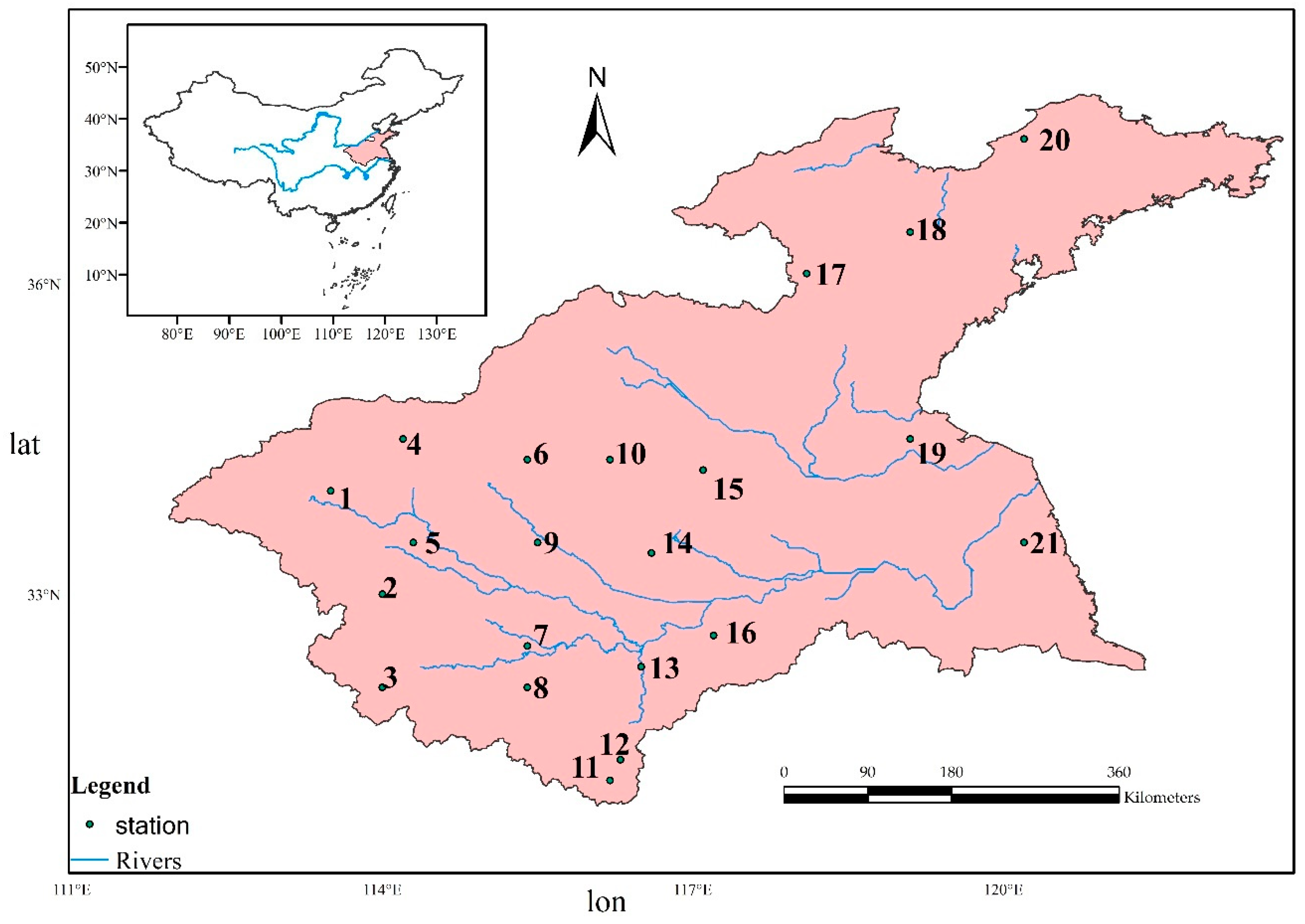
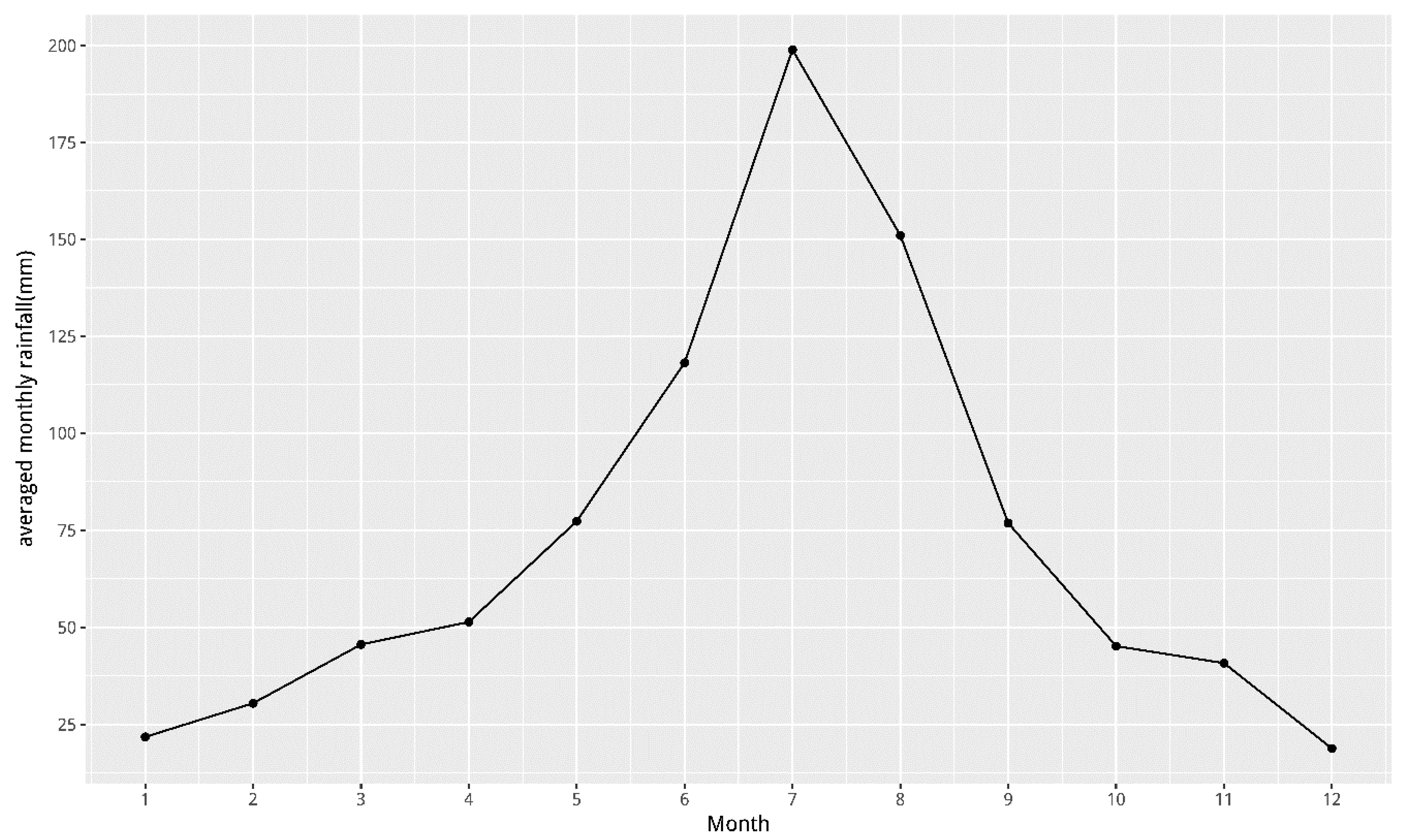
The Huaihe River Basin (HRB) ( and ) shown in Figure 1, with an area of 270,000 km2, is one of the most densely inhabited areas in China. The HRB is a significant crop area in China due to its special climate, which is characterized by warm temperate climate in the northern part and subtropical climate in the southern part. Wheat and grain production accounts for about 50% and 20% of the country’s total, respectively. The rainy season plays an important role in crop planting in the HRB. It can be pointed out from Figure 2 that rainy-season precipitation (generally from May–September in the HRB) accounts for the largest part of the annual total precipitation [25]. Consequently, investigation and prediction of rainy-season precipitation are of central importance for this area.
2.2. Data Description
Daily rainfall data from 1987–2016 at 21 rainfall stations were chosen to explore rainy-season precipitation in this study. Detailed location information (longitude, latitude, and elevation) for these stations and average rainy season features (onset, retreat of rainy season, and rainy-season precipitation) for the period of 1987–2016 are listed in Table 1. The average onset (retreat) of rainy season for the 21 rainfall stations in 1987–2016 is Julian Day 134 (258), which is selected as the rainy-season period for predicting precipitation in this study.
The precipitation data were provided by the China Meteorological Data Sharing Service System [26], which is also responsible for quality control. Vector wind data were obtained from the National Center for Environmental Prediction/National Center for Atmospheric Research (NCEP/NCAR) in order to explore the underlying causes of the determined hidden states in the model [27]. The atmospheric circulation and monsoon could change sea surface temperature anomalies (SSTA) patterns, which could affect precipitation in the HRB [20]. There are many SSTA-related indices, such as Indian Ocean Dipole (IOD), Summer North Atlantic Oscillation (SNAO), and Niño 1–2, which are used to represent SSTA in different ocean regions. They all have large influences on rainfall in the HRB. SSTA-related indices data were provided by the Koningklijk Nederlands Meterologisch Instituut (KNMI) climate explorer database to identify candidate atmospheric predictors in the Bayesian-NHMM [28].
3. Methods
3.1. Determination of Rainy Season
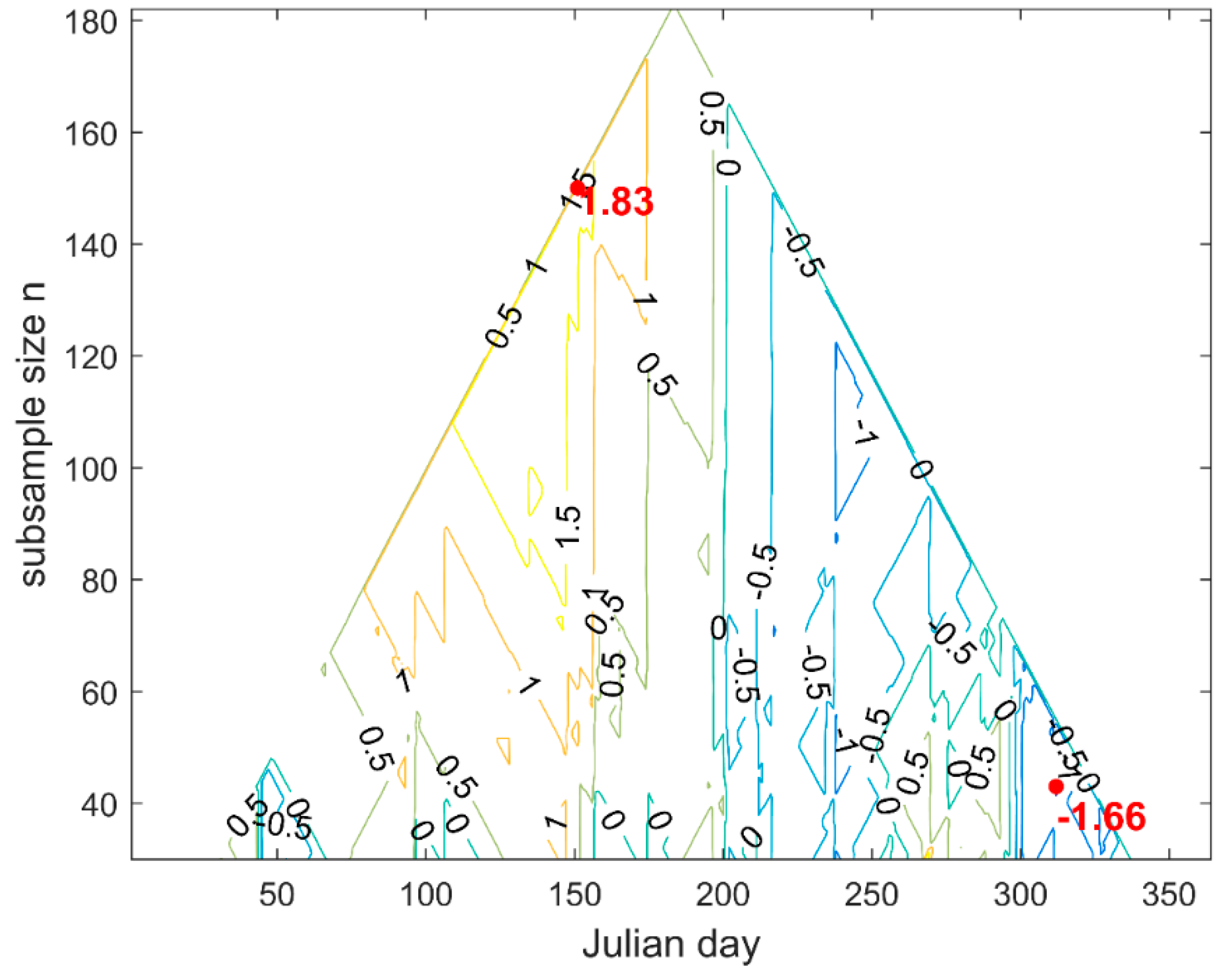
There is, in general, no straightforward and unique method for determination of the length of rainy season. Most methods are somewhat subjective because they are based on threshold values of given indices to identify the rainy season, such as rainfall, monsoon, or temperature [29,30]. However, the moving t-test method applied in this study, which has been used by many researchers (e.g., Cao et al. [31]), does not need an ad hoc threshold. The method is characterized by identifying a breaking point between two samples. The two samples have equal size before and after the breaking point according to [32,33]:
where , defined as:
where xi is daily precipitation data for Julian day i in one year at one station in the HRB. and are averaged values of two subsamples before and after Julian day i, respectively. n is the length of each subsample.
The t-value was normalized by the 0.01 significance test shown in Equation (4), which is equal to the Mann-Kendall test at the 0.05 significance level:
where is the threshold to detect onset and retreat of rainy season. Onset is the Julian day i corresponding to the maximum , with rainfall changing from a small to a large value. Similarly, retreat was evaluated by the minimum
The Xuchang Station (station 1) in the HRB is used as an example to show the determination of rainy season (Figure 3). The yellow-greenish lines present positive values and blue lines show negative values. The maximum is 1.83 when the Julian day is 151 and the timescale is 150. It means the most prominent abruption point is Julian day 151, which is also the onset of the rainy season, in the timescale of 150 days. Similarly, retreat of the rainy season in 2016 at station 1 is 312 in a timescale of 182 days.
3.2. The Bayesian Homogeneous Markov Model
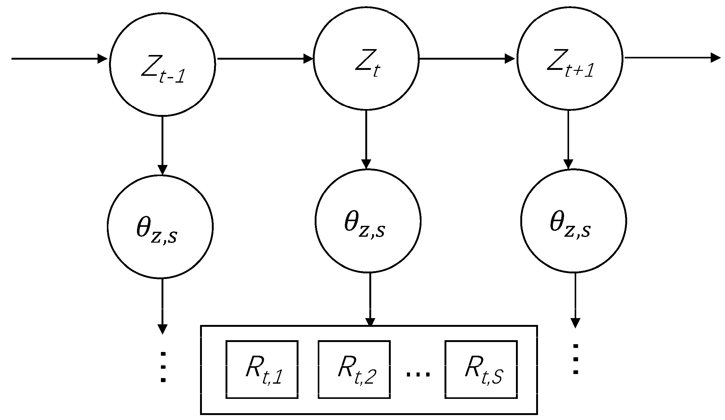
A Bayesian-HMM is a stochastic model where data are generated conditionally on several discrete hidden states by a certain probability distribution. These underlying hidden states undergo Markovian transition. In terms of hydrological application, a hidden state could be considered as an unobserved weather variable, which affects precipitation occurrence and amount at many stations in a region at the same time. In this study, the Bayesian-HMM could present a probabilistic framework of the joint distribution of rainy-season precipitation at a daily time scale at the 21 rainfall stations in the HRB. Figure 4 demonstrates the model network where dependencies are denoted by arrows and time flow from left to right at an increment. refers to daily rainy-season precipitation at s(s = 1,2, … , S) station at time t. is a hidden Markov state variable in time t, with Z ranging from 1 to K. K is the total number of hidden states. is the set for all parameters in a spatial rainfall distribution, specific to hidden state z and station s.
Two assumptions are made for a Bayesian-HMM. The first is that hidden states are first-order Markov processes and the K × K state-to-state probability matrix Q in Equation (5) does not change in time:
The second assumption is that the observations at time t are conditionally independent of observations and states of other days up to time t, as shown in Equation (6):
where is observed precipitation during rainy season during time t for S rainfall stations (S = 21 in this study). Based on both assumptions, the conditional likelihood of the Bayesian-HMM can be written as:
where represents the initial state distribution.
3.3. Bayesian Nonhomogeneous Markov Model
The Bayesian-NHMM is extended by introducing additional observed values into the transition matrix of the Bayesian-HMM to allow each transition to have specific logistic coefficients. As a consequence, precipitation is dependent on observed input variables. The matrix in the Bayesian-NHMM is a nonhomogeneous transition matrix with components , which can be calculated as:
where represents a sequence of p exogenous atmospheric variables at time t, which are related to rainy-season precipitation. is a p-dimensional vector of coefficients related to . Let for convenience.
The other main component in a Bayesian-NHMM is state-dependent emission distributions , where is the set of all parameters of emission distributions, specific to hidden state z and station s. Generally, these distributions are also nonhomogeneous over time because is dependent on station-level variables . represents exogenous variables at time t related to rainfall stations, such as longitude, latitude, and Julian days. A delta function and a mixture of two gamma distributions are applied to fit dry days and rainfall amounts on wet days [34,35].
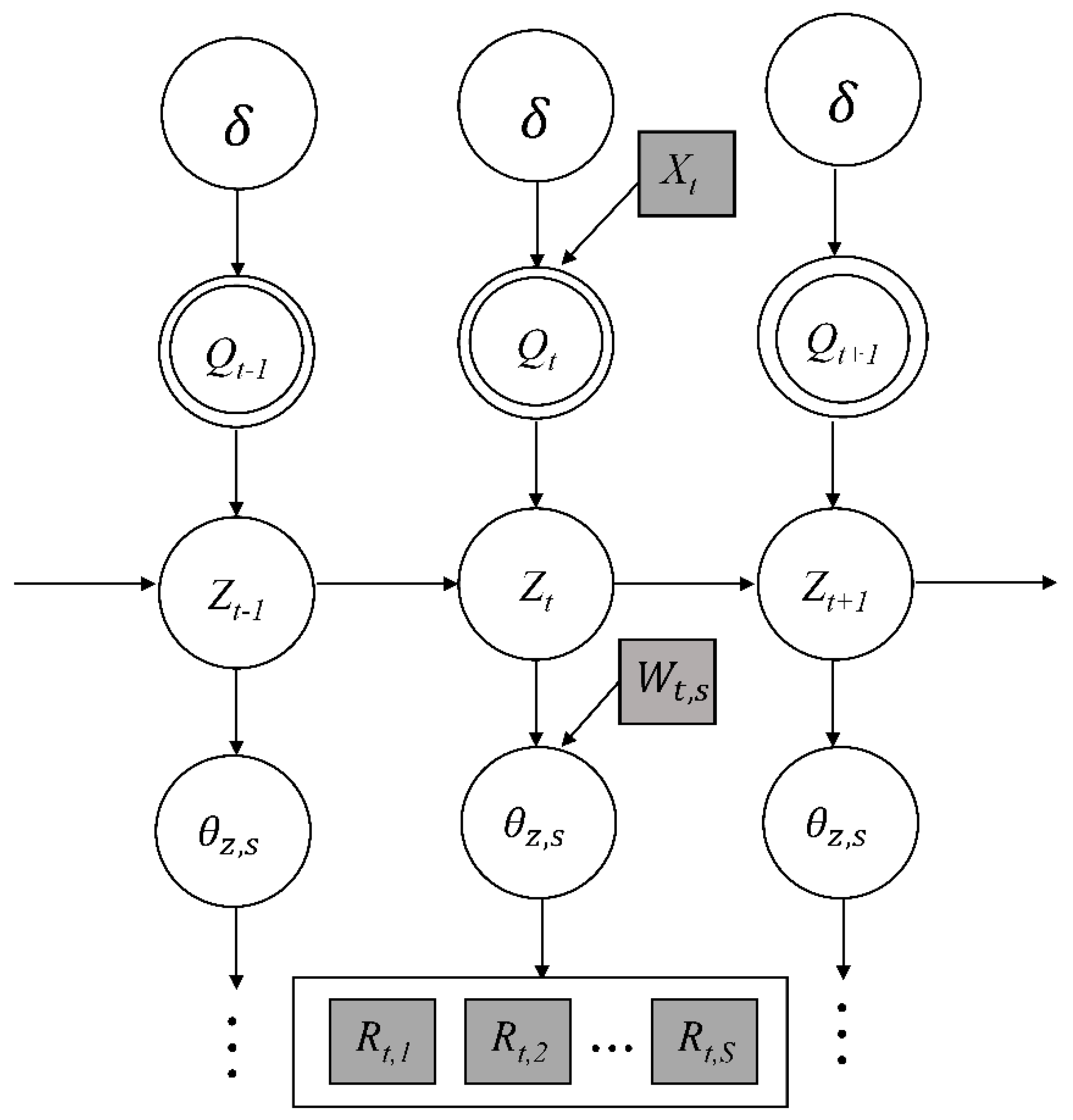
Figure 5 presents the Bayesian-NHMM network and how the two types of exogenous variables () affect the model. The conditional likelihood of data in the Bayesian-NHMM can be written as:
Estimation begins with Bayes’ conditional probability theory:
where refers to all parameters in the model and R is the rainfall sequence. is an unconditional distribution, representing our knowledge of prior to R. is the likelihood function, and represents the posterior density.
For simple problems Equation (10) can have analytical solutions, but closed-form solutions do not exist for complex models. As a consequence, Markov Chain Monte Carlo (MCMC) methods are used to provide samples from the posterior densities of interest. The detailed process on how to use MCMC in the Bayesian-NHMM is presented by Holsclaw et al. [19].
4. Results and Discussion
Below, steps to construct the models are briefly described. First, the Bayesian-HMM is run to identify spatial dependence between different rainfall stations in the HRB and different number of hidden states. The optimal Bayesian-HMM is chosen by comparing log-likelihood among models with different number of hidden states. In this phase, daily rainfall amount and rainfall occurrence probability for different states are calculated. The temporal sequence of hidden states of Bayesian-HMM is then calculated by the Viterbi algorithm. The Viterbi algorithm could find the state sequence where is maximum and identify the most probable sequence of rainfall states [36,37]. The detailed dynamic programming algorithm is provided by Kirshner [38].
Then, the relationship between meteorological elements and rainy-season precipitation corresponding to different hidden states is explored to explain the underlying causes of different rainfall patterns in the different hidden states.
Finally, analysis of potential predictors is performed in the Bayesian-NHMM. The Bayesian-NHMM is fitted to different combinations of candidate predictors (SSTA-related indices, such as IDO, SNAO). Evaluation of all models is carried out by five-fold cross-validation, where five different consecutive six-year blocks of data are used in turn and models are fitted to the other 24 years of data. For each model, 1000 predictive runs for each of the six-year blocks are generated. The ability to simulate seasonality and interannual variability of rainfall is evaluated among different models.
4.1. Identification of Hidden States and Spatial Precipitation Dependence
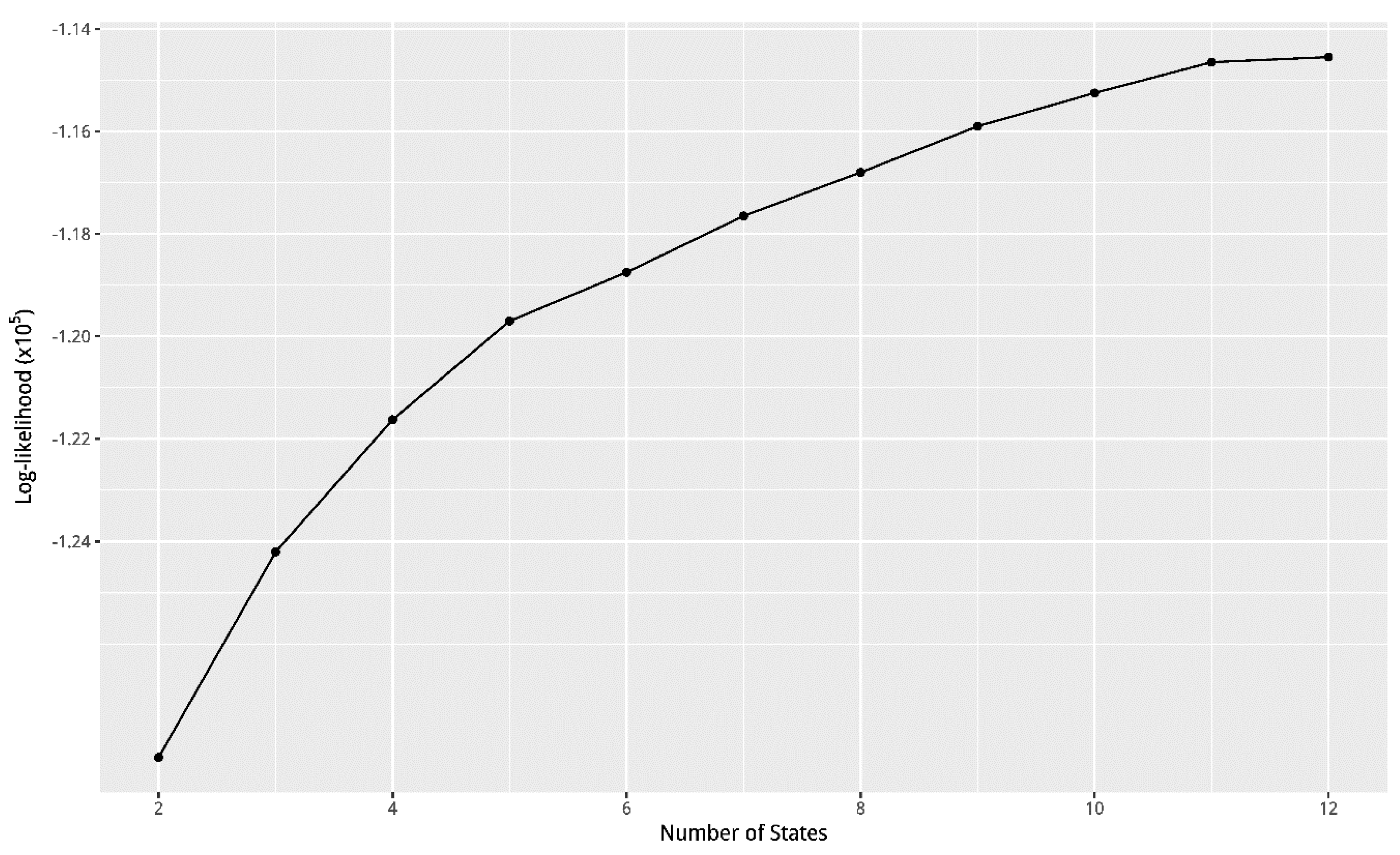
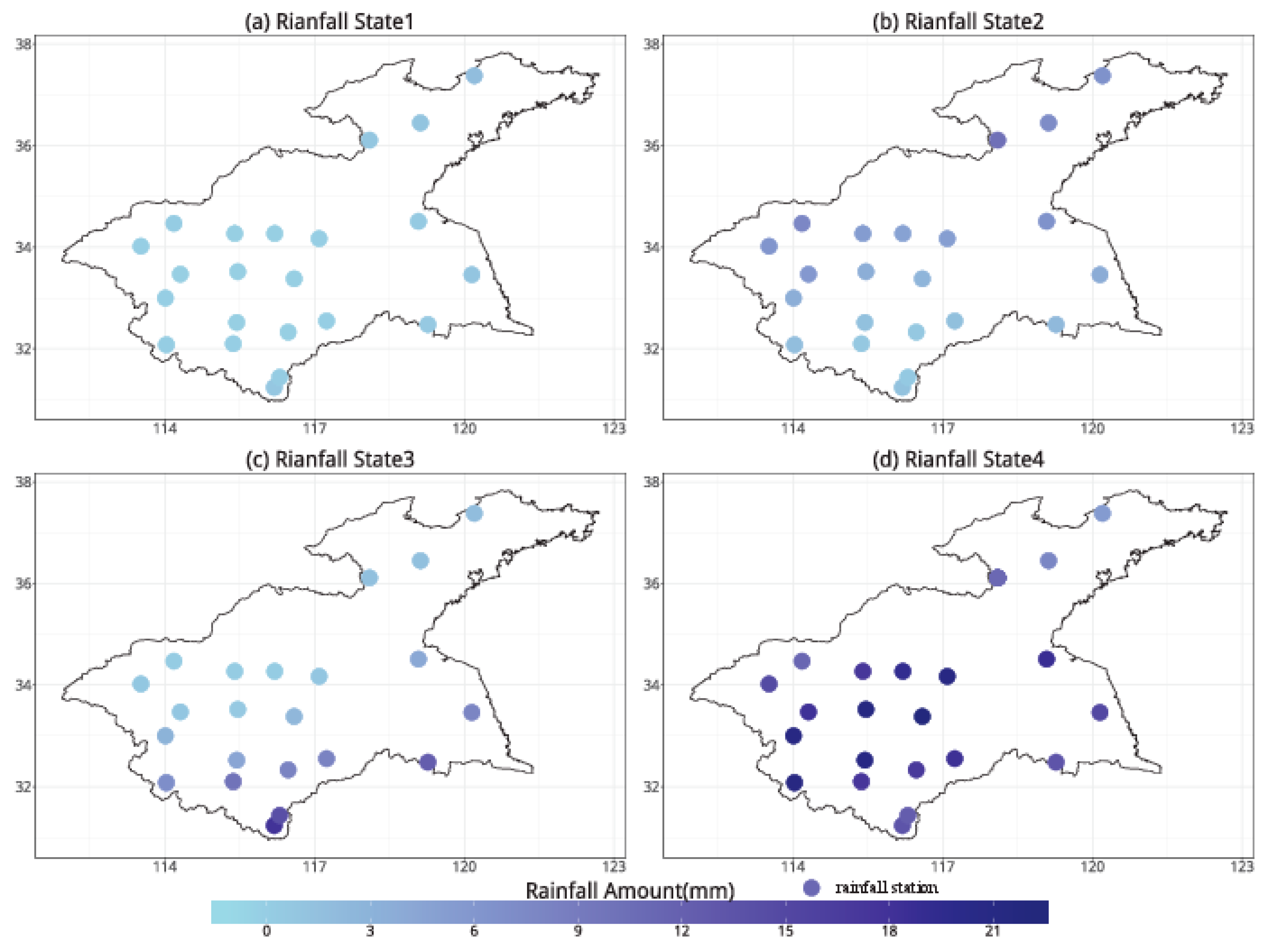
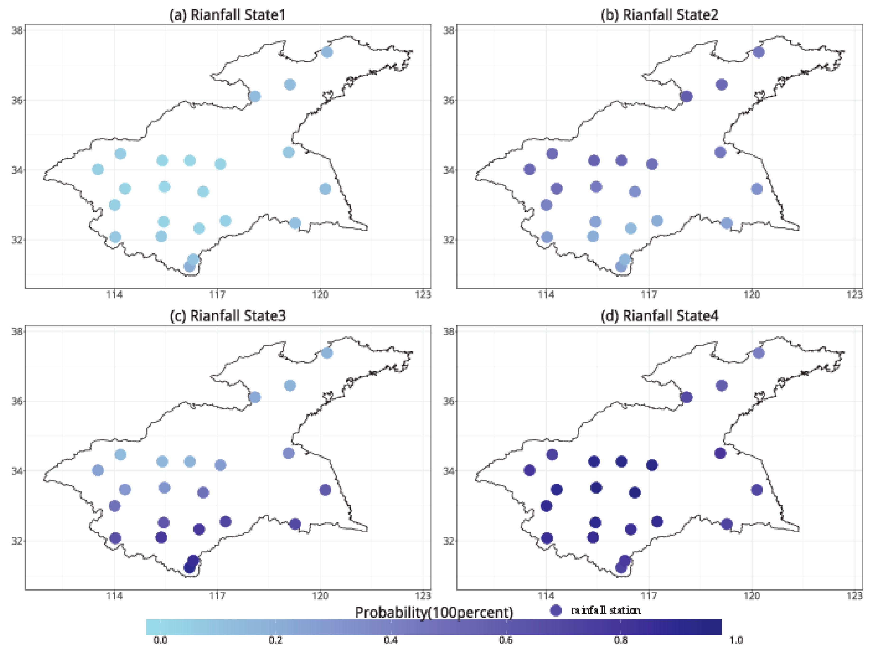
The number of hidden states has a considerable effect on model performance. The selection of appropriate number of hidden states k in the Bayesian-HMM was guided by calculating log-likelihood of models with different choices of k under fivefold cross validation (shown in Figure 6). Log-likelihood is often applied to determine the number of hidden states (e.g., Robertson et al. [35]). As shown in Figure 6, the log-likelihood increases sharply initially before k = 4/5 and then levels off. As a consequence, the daily rainfall amount and rainfall occurrence probability for the four-state model (shown in Figure 6 and Figure 7) and the five-state model (shown in Figures S1 and S2) are compared. In Figure 6 and Figure 7, the dots in the four-panel figures demonstrate not only the location of rainfall stations but also the magnitude of daily precipitation amount vs. rainfall occurrence probability. The darker dots indicate larger rainfall amount during rainy season/rainfall occurrence probability. It can be seen from Figure 7 that State 1 represents dry days during rainy season. State 2 demonstrates days with small rainfall amount in the southern part of the HRB, with the northern HRB showing a wetter signal. In contrast, State 3 represents large (small) rainy-season precipitation in the southern (northern) region of the HRB. State 4 demonstrates days with a large amount of rainy-season rainfall for all stations. The occurrence probability for the four states is shown in Figure 8, which corresponds to Figure 7. States 1 and 4 show the smallest, and largest precipitation occurrence probability, respectively. State 2 demonstrates more probable rainfall in the northern HRB and less in the southern HRB, while State 3 shows the opposite situation. In Figure S1, patterns of daily rainfall amount for five states are presented. States 1–3 show similar patterns and all represent dry days during rainy season. State 4 shows wet signals in the southern part of the HRB, with the northern HRB presenting dry signals. State 5 demonstrates wet signals for all stations. In Figure S2, States 2 and State 4 also show similar patterns for rainfall occurrence probabilities. It can be pointed out that the difference among states in the five-state model is not that clear as compared to the four-state model. Consequently, the four-state model was chosen in this study.
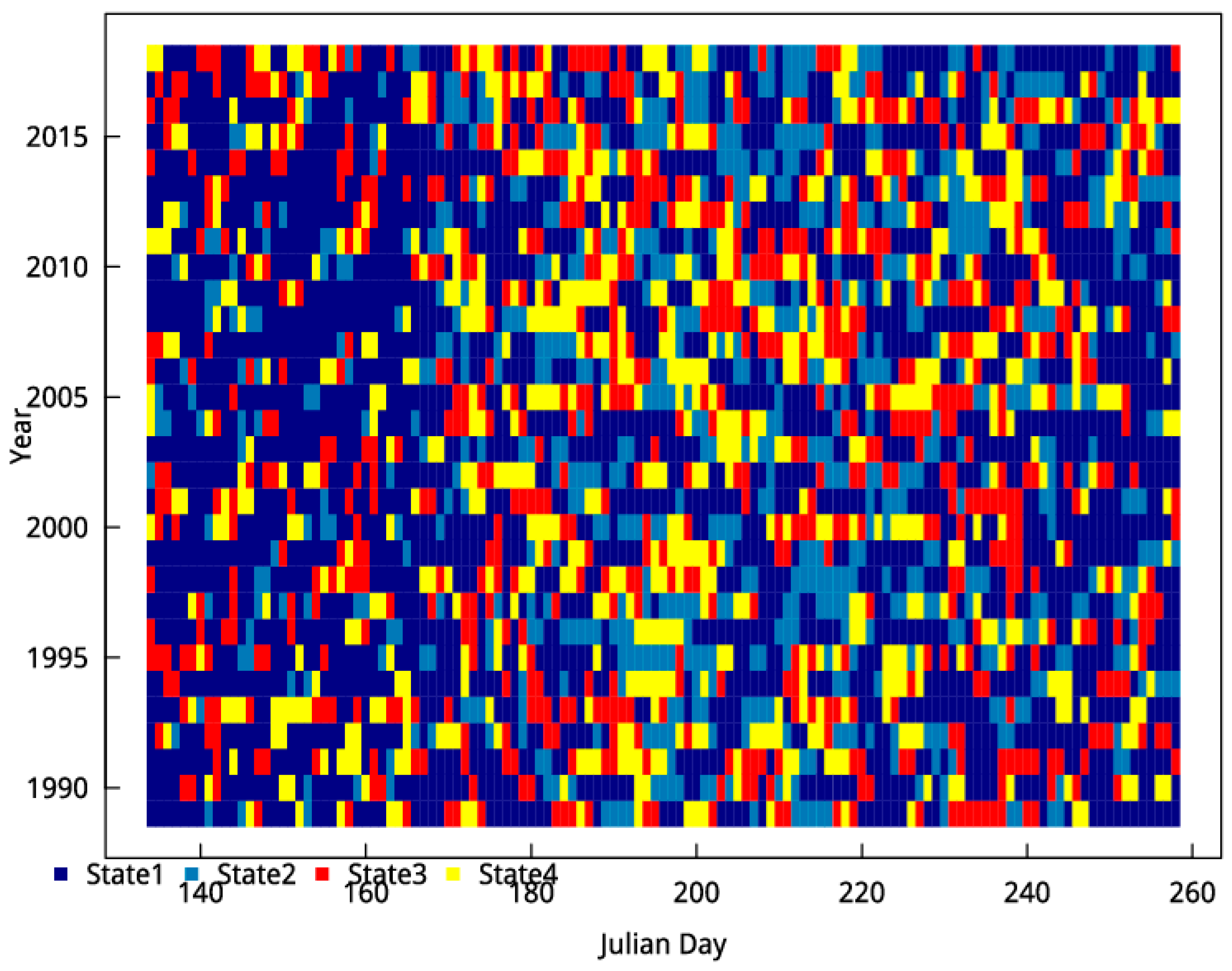
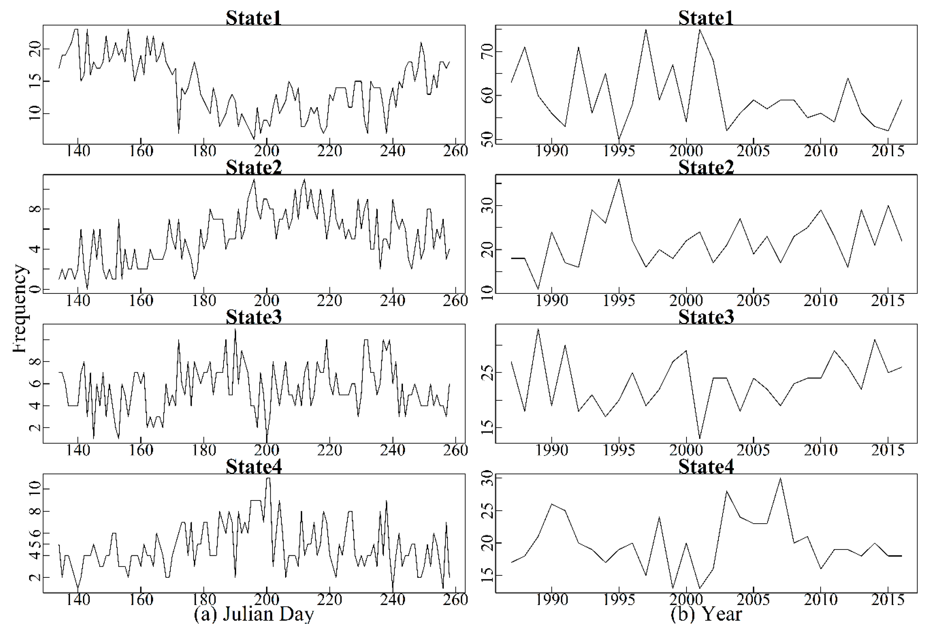
The most likely daily series of the four states described above are plotted in Figure 9. In general, Figure 9 suggests that precipitation sequences present considerable variability in terms of rainfall amount and occurrence probability for both seasonal (horizontally in Figure 9) and interannual time scale (vertically in Figure 9), which is demonstrated in detail in Figure 10. As shown in Figure 10, the frequency of State 1 decreased from onset of rainy season to the middle phase and then increased. The frequency of States 2 and 4 was highest in the middle phase of the rainy season, with State 3 showing no obvious trend. At the interannual scale, the frequency of State 1 fluctuated before year 2003, followed by an obvious downward trend. States 2 and 3 reached generally stable levels. State 4 showed a downward tendency before year 2003, with an upward trend from 2003 to 2007. The frequency reached a peak at 2007 and then stabilized.
State 4 (the wettest state) showed high frequency in 2003 and 2007, with State 1 presenting obvious small frequency, which could contribute to floods. According to previous research, heavy floods occurred in July 2003 in the HRB, with the largest flood during 91 years [39,40,41,42]. Similarly, heavy floods occurred over the entire HRB in 2007 [39,43,44].
Summarized from Figure 6, Figure 7, Figure 8 and Figure 9, State 1 represents a dry homogeneous signal for all stations, which is dominant near the onset and retreat of rainy season. State 2 is a wet, but nonhomogeneous, condition mainly in the middle phase of rainy season. In this case, there is larger precipitation in the northern part of the HRB. State 3 is also a nonhomogeneous wet condition, but larger rainfall is shown in the southern HRB. State 4 could be defined as a very wet homogenous condition for all stations, which is dominant in the middle phase of rainy season.
4.2. Meteorological Patterns Associated with the Hidden States
Each particular day can be classified into one of the hidden weather states in the Bayesian-HMM. Averaged atmospheric circulation over common-state days can present a physical linkage between weather states and atmospheric forcing factors. To gain insight into precipitation patterns related to weather states, we averaged wind vectors and moisture flux over days classified into one state.
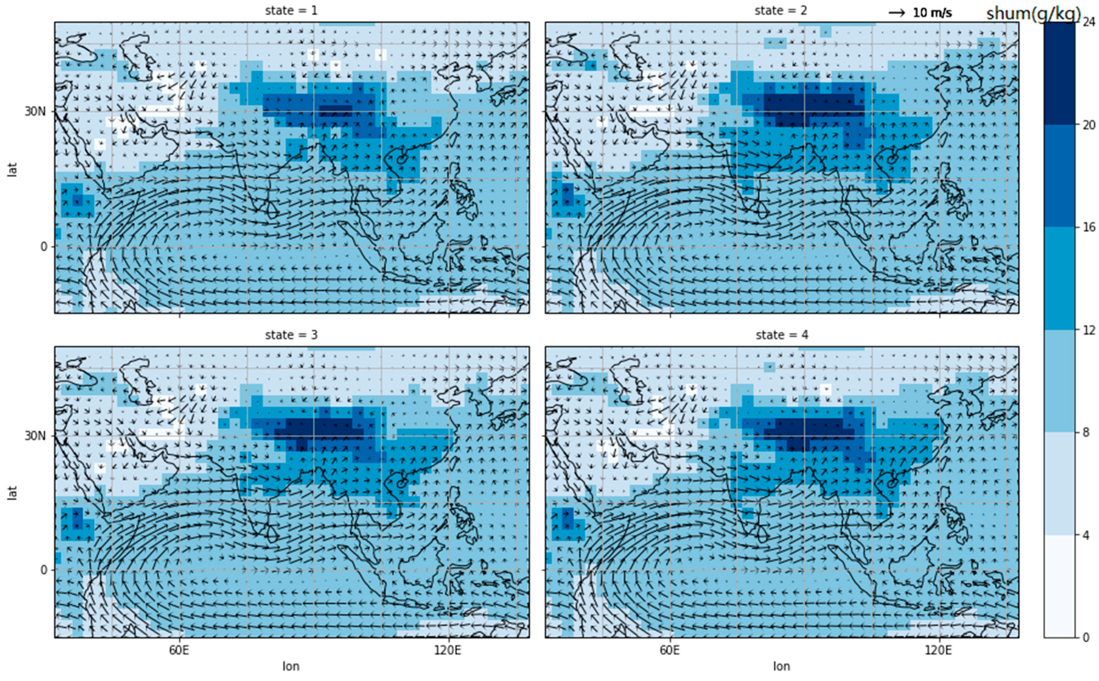
Figure 11 shows composite atmospheric anomalies for four hidden states at 850 hPa geopotential height. Li et al. [21] performed a comparison among circulation patterns at 200, 500, and 850 hPa in the HRB and pointed out that heavy rainfall is mainly associated with wind anomalies at the 850 hPa level. As shown in Figure 11, State 1 presented weakest moisture flux and monsoon near the HRB, which is consistent with results showing that State 1 has the smallest rainfall. State 2 shows a similar circulation pattern to State 3, both with stronger monsoon and increased moisture flux as compared to State 1. State 4 is most frequent in the middle phase of rainy season (Figure 10) and is representative of the strongest monsoon. Zhang et al. [39] analyzed the effects of ENSO on seasonal precipitation in the HRB and used the water vapor flux maps to explore the underlying causes of ENSO-related precipitation. They pointed out that water vapor corresponds to the amount of rainfall in the HRB. Active water vapor could bring enough precipitation to the HRB. Cao et al. [45] analyzed the influence of monsoon on rainy-season precipitation in the HRB. Stronger monsoons from the Indian Ocean are related to more rainfall in the HRB. The underlying causes of different rainfall states shown in this study are associated with monsoon and water vapor flux. Stronger monsoons and active water vapor correspond to wetter states in the HRB, which are consistent with their research.
4.3. Bayesian-NHMM Calibration and Validation
4.3.1. Selection of Potential Predictors for Bayesian-NHMM
The first step to build the Bayesian-NHMM is to select potential predictors. Much research has analyzed the influence of El Niño-Southern Oscillation (ENSO) on precipitation over the HRB [20,39,46,47,48,49]. Wang et al. [20] studied spatial and temporal patterns of rainfall over the HRB. They established a possible link between rainfall and different ENSO events, such as in the Eastern Pacific [21], found that heavy precipitation is affected by SSTA over the equatorial Western Pacific and the Northern Indian Ocean. As a consequence, Niño indices (i.e., Niño 1–2, Niño 3, Niño 3.4, Niño 4), which are used to define different types of ENSO, were chosen as candidate predictors in the Bayesian-NHMM. In addition, Liu et al. [47] pointed out that the influence of ENSO on rainfall over the HRB is offsetting the relationship between the IOD and summer rainfall. Other researchers argued that Pacific Decadal Oscillation (PDO), North Atlantic Oscillation (NAO), SNAO also have important effects on precipitation in the HRB [50,51,52,53,54]. IOD, PDO, NAO, and SNAO, therefore, were also selected as candidate predictors. In Table 2, correlation between candidate predictors and rainy-season precipitation is listed. Considering that large-scale climate indices have lagged influence on region-scale rainfall, relationships between rainy-season rainfall and candidate predictors with a lag ranging between 1 and 12 months were calculated. Lag combinations with the strongest correlation for each predictor are listed in Table 2. Three predictors (IOD, SNAO, and Niño 1–2) were chosen, with the absolute value of rs larger than 0.3 and p-value smaller than 0.1, in order to guarantee that correlation between rainfall and climate indices is strong and that results are significant at the 0.1 significance level.
In Table 3, models together with their corresponding combinations of predictors are listed. The result of Bayesian-HMM to predict rainfall was calculated to compare with the Bayesian-NHMM.
4.3.2. Seasonality
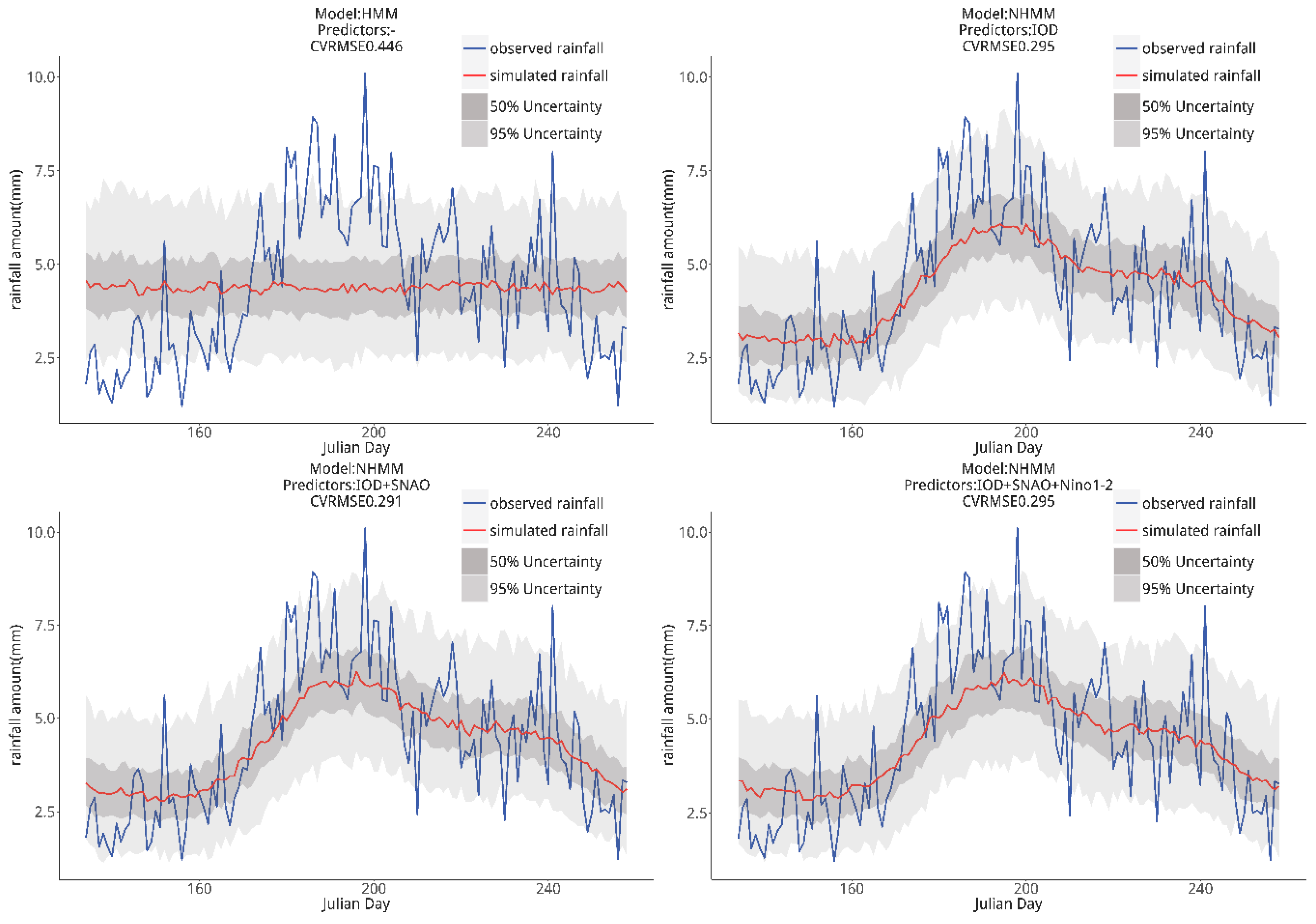
The quality of selected models to reproduce the seasonal cycle of rainfall is illustrated in Figure 12. The blue line shows the seasonality of observed rainy-season precipitation, obtained by averaging precipitation for all stations and each day during the rainy season for 30 years. The red line presents simulated mean rainy-season precipitation. The range of variation from 1000 simulations in each model is presented by the shaded area, which interprets the inter-quartile range. The coefficient of variation of root mean squared error (CVRMSE) of each model is calculated in order to provide an estimate of the difference in the performance of the models. CVRMSE is defined as:
where is mean rainy-season rainfall from simulations, is mean rainy-season rainfall from observations, and is the number of years.
From Figure 12, it is clear that the Bayesian-HMM cannot reproduce the seasonal cycle of rainy-season precipitation in the HRB, but the seasonality is well captured by the different Bayesian-NHMMs based on the set of predictors. This means the Bayesian-NHMM can be efficient in predicting future change of rainfall seasonality. The Bayesian-NHMM model with predictors DMI and SNAO is better in reproducing the typical seasonal precipitation during rainy season than the other two Bayesian-NHMMs, considering its smaller CVRMSE value.
4.3.3. Interannual Variability
In this section, the ability of different Bayesian-HMM and Bayesian-NHMMs to capture interannual variability of rainfall amount and wet days during rainy season is evaluated. Figure 13 demonstrates a comparison between interannual variability of observed and simulated rainfall amount. The blue line shows observed rainy-season precipitation at the interannual scale, obtained by averaging rainy-season precipitation for all stations and each year. The red line presents mean simulated rainy-season precipitation for each year. The range of variation from 1000 simulations for each model is presented by the shaded area, which interprets the inter-quartile range.
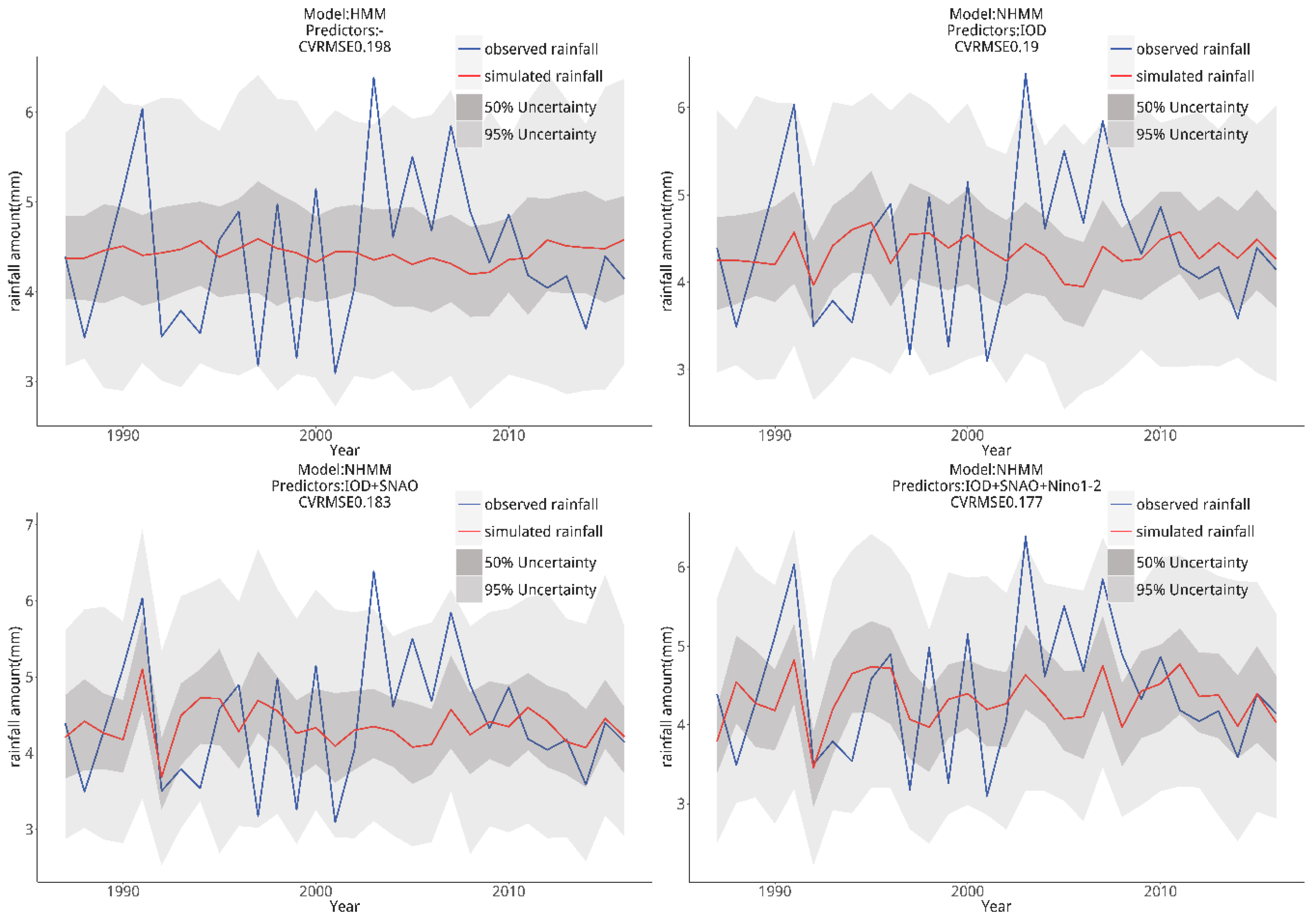
As seen from Figure 13, the Bayesian-HMM cannot capture the interannual variation of rainy-season precipitation. The Bayesian-NHMM with three predictors (DMI, SNAO, and Niño 1–2) fits the observations better as compared to models with one or two predictors. The CVRMSE is presented in the figure to make a more complete analysis. It can be pointed out that the three-predictor Bayesian-NHMM has the smallest CVRMSE value (0.177), showing its better performance in simulating interannual rainfall amount during the rainy season.
Figure 14 demonstrates a comparison between interannual variability of observed and simulated wet days during rainy season. Similarly, the performance of the Bayesian-HMM is worst and the Bayesian-NHMM with three predictors presents the best ability to capture wet days during rainy season at the interannual scale.
5. Conclusions
A new approach (Bayesian-NHMM) to simulate multisite rainfall in the HRB was presented in this study. As compared to the traditional NHMM, the model allows for exogenous variables to affect both transition probabilities of hidden states and emission distribution. In addition, sampling was done in the Bayesian-NHMM by a data augmentation method that removed the need to tune parameters.
The Bayesian-HMM was first used to analyze rainfall pattern during rainy season in the HRB for 21 precipitation stations during 1987–2016. A four-state model was chosen from analysis of log-likelihood of precipitation in the model. The Viterbi algorithm was applied to show temporal evolution of hidden states driving the observed rainfall. Heavy precipitation state is related to strong monsoon from the Indian Ocean that brings large amounts of moisture to the HRB.
The Bayesian-NHMM was then used to successfully downscale and simulate precipitation based on atmospheric predictors. The performance of models with different combination of predictors (IOD; IOD + SNAO; IOD+SNAO + Niño 1–2) were evaluated in terms of their ability to capture seasonality and interannual variability of rainfall.
The results show that the Bayesian-NHMM is better to capture such variations as compared to the Bayesian-HMM, because precipitation was conditioned on atmospheric information. In general, the Bayesian-NHMMs with different predictors are better to capture most local precipitation patterns. The distributional properties of rainfall, such as seasonal cycle of rainfall amount and interannual variability of rainfall amount and wet days during the rainy season, were well presented by the Bayesian-NHMM.
Supplementary Materials
The following are available online at https://www.mdpi.com/2073-4441/11/5/916/s1, Figure S1: Daily rainfall amount for five states, the dots in the figure demonstrate not only the location of rainfall stations but also the magnitude of daily precipitation amount, Figure S2: Occurrence probability for five states, the dots in the figure demonstrate not only the location of rainfall stations but also the magnitude of rainfall occurrence probability.
Author Contributions
Conceptualization, Q.C.; methodology, Z.H.; software, S.X.; validation, R.B., F.Y.; formal analysis, H.G.; investigation, Q.C.; resources, J.H.; data curation, S.X.; writing—original draft preparation, Q.C.; writing—review and editing, Q.C.; visualization, Q.C.; supervision, F.Y.; project administration, Z.H.; funding acquisition, Z.H.
Funding
This work was supported by the Supported by the National Key Research Projects (grant no. 2018YFC1508001), National Key R&D Program of China (grant no. 2016YFC0402704) and the Fundamental Research Funds for the Central Universities (grant ID 2018B41214).
Acknowledgments
The author Qing Cao also acknowledges support from the China Scholarship Council. The authors would also thank the anonymous reviewers for their constructive comments, which greatly helped improve this paper.
Conflicts of Interest
The authors declare no conflict of interest.
References
- Khalil, A.F.; Kwon, H.-H.; Lall, U.; Kaheil, Y.H. Predictive downscaling based on non-homogeneous hidden markov models. Hydrolog. Sci. J. 2010, 55, 333–350. [Google Scholar] [CrossRef]
- Hewitson, B.; Crane, R. Climate downscaling: Techniques and application. Clim. Res. 1996, 7, 85–95. [Google Scholar] [CrossRef]
- Zorita, E.; Von Storch, H. The analog method as a simple statistical downscaling technique: Comparison with more complicated methods. J. Clim. 1999, 12, 2474–2489. [Google Scholar] [CrossRef]
- Maraun, D.; Wetterhall, F.; Ireson, A.; Chandler, R.; Kendon, E.; Widmann, M.; Brienen, S.; Rust, H.; Sauter, T.; Themeßl, M. Precipitation downscaling under climate change: Recent developments to bridge the gap between dynamical models and the end user. Rev. Geophys. 2010, 48. [Google Scholar] [CrossRef]
- Giorgi, F.; Mearns, L.O. Calculation of average, uncertainty range, and reliability of regional climate changes from aogcm simulations via the “reliability ensemble averaging”(rea) method. J. Clim. 2002, 15, 1141–1158. [Google Scholar] [CrossRef]
- Von Storch, H. Regional climate development under global warming. General technical report no. 4. In Review of Empirical Downscaling Techniques; GKSS Research Center: Hamburg, Germany, 2000. [Google Scholar]
- Fowler, H.J.; Blenkinsop, S.; Tebaldi, C. Linking climate change modelling to impacts studies: Recent advances in downscaling techniques for hydrological modelling. Int. J. Climatol. 2007, 27, 1547–1578. [Google Scholar] [CrossRef]
- Hashmi, M.; Shamseldin, A.; Melville, B. Statistical downscaling of precipitation: State-of-the-art and application of bayesian multi-model approach for uncertainty assessment. Hydrol. Earth Syst. Sci. Discuss. 2009, 6, 6535–6579. [Google Scholar] [CrossRef]
- Wilby, R.L.; Charles, S.; Zorita, E.; Timbal, B.; Whetton, P.; Mearns, L. Guidelines for use of climate scenarios developed from statistical downscaling methods. Available online: http://www.ipcc-data.org/guidelines/dgm_no2_v1_09_2004.pdf (accessed on 30 April 2019).
- Robertson, A.W.; Kirshner, S.; Smyth, P.; Charles, S.P.; Bates, B.C. Subseasonal-to-interdecadal variability of the Australian monsoon over north queensland. Q. J. R. Meteor. Soc. 2006, 132, 519–542. [Google Scholar] [CrossRef]
- Robertson, A.W.; Kirshner, S.; Smyth, P. Downscaling of daily rainfall occurrence over northeast Brazil using a hidden markov model. J. Clim. 2004, 17, 4407–4424. [Google Scholar] [CrossRef]
- Robertson, A.W.; Kirshner, S.; Smyth, P. Hidden Markov Models for Modeling Daily Rainfall Occurrence over Brazil; University of California: San Francisco, CA, USA, 2003. [Google Scholar]
- Lianyi, G.; JIANG, Z.; Weilin, C. Using a hidden markov model to analyze the flood-season rainfall pattern and its temporal variation over east China. J. Meteor. Res. 2018, 32, 410–420. [Google Scholar]
- Cioffi, F.; Conticello, F.; Lall, U.; Marotta, L.; Telesca, V. Large scale climate and rainfall seasonality in a mediterranean area: Insights from a non-homogeneous markov model applied to the agro-pontino plain. Hydrol. Process. 2017, 31, 668–686. [Google Scholar] [CrossRef]
- Pal, I.; Robertson, A.W.; Lall, U.; Cane, M.A. Modeling winter rainfall in northwest india using a hidden markov model: Understanding occurrence of different states and their dynamical connections. Clim. Dyn. 2015, 44, 1003–1015. [Google Scholar] [CrossRef]
- Städler, N.; Mukherjee, S. Penalized estimation in high-dimensional hidden markov models with state–specific graphical models. Ann. Appl. Stat. 2013, 2157–2179. [Google Scholar] [CrossRef]
- Greene, A.M.; Holsclaw, T.; Robertson, A.W.; Smyth, P. A bayesian multivariate nonhomogeneous markov model. In Machine Learning and Data Mining Approaches to Climate Science; Springer: New York, NY, USA, 2015; pp. 61–69. [Google Scholar]
- Holsclaw, T.; Greene, A.M.; Robertson, A.W.; Smyth, P. A bayesian hidden markov model of daily precipitation over South and East Asia. J. Hydrometeorol. 2016, 17, 3–25. [Google Scholar] [CrossRef]
- Holsclaw, T.; Greene, A.M.; Robertson, A.W.; Smyth, P. Bayesian nonhomogeneous markov models via pólya-gamma data augmentation with applications to rainfall modeling. Ann. Appl. Stat. 2017, 11, 393–426. [Google Scholar] [CrossRef]
- Wang, Y.; Zhang, Q.; Singh, V.P. Spatiotemporal patterns of precipitation regimes in the Huai River Basin, China, and possible relations with Enso events. Nat. Hazards 2016, 82, 2167–2185. [Google Scholar] [CrossRef]
- Li, L.; Li, W.; Tang, Q.; Zhang, P.; Liu, Y. Warm season heavy rainfall events over the Huaihe River valley and their linkage with wintertime thermal condition of the tropical oceans. Clim. Dyn. 2016, 46, 71–82. [Google Scholar]
- Xiao, M.; Zhang, Q.; Singh, V.P.; Chen, X. Probabilistic forecasting of seasonal drought behaviors in the Huai River Basin, China. Theor. Appl. Climatol. 2017, 128, 667–677. [Google Scholar] [CrossRef]
- Yan, D.; Wu, D.; Huang, R.; Wang, L.; Yang, G. Drought evolution characteristics and precipitation intensity changes during alternating dry–wet changes in the Huang–Huai–Hai River Basin. Hydrol. Earth Syst. Sci. 2013, 17, 2859–2871. [Google Scholar] [CrossRef]
- Chen, X.; Hao, Z.; Devineni, N.; Lall, U. Climate information based streamflow and rainfall forecasts for Huai River Basin using hierarchical bayesian modeling. Hydrol. Earth Syst. Sci. 2014, 18, 1539–1548. [Google Scholar] [CrossRef]
- Yang, M.; Chen, X.; Cheng, C.S. Hydrological impacts of precipitation extremes in the Huaihe River Basin, China. SpringerPlus 2016, 5, 1731. [Google Scholar]
- The China meteorological data sharing service system. Available online: http://data.cma.cn/data/detail/dataCode/SURF_CLI_CHN_MUL_DAY_V3.0.html (accessed on 30 April 2019).
- Kalnay, E.; Kanamitsu, M.; Kistler, R.; Collins, W.; Deaven, D.; Gandin, L.; Iredell, M.; Saha, S.; White, G.; Woollen, J.; et al. The ncep/ncar 40-year reanalysis project. Bull. Am. Meteor. Soc. 1996, 77, 437–471. [Google Scholar] [CrossRef]
- The koningklijk nederlands meterologisch instituut (knmi) climate explorer database. Available online: http://climexp.knmi.nl/ (accessed on 30 April 2019).
- Goswami, B.; Xavier, P.K. Enso control on the south asian monsoon through the length of the rainy season. Geophys. Res. Lett. 2005, 32. [Google Scholar] [CrossRef]
- Reason, C.J.C.; Hachigonta, S.; Phaladi, R.F. Interannual variability in rainy season characteristics over the Limpopo region of Southern Africa. Int. J. Climatol. 2005, 25, 1835–1853. [Google Scholar] [CrossRef]
- Cao, Q.; Hao, Z.; Yuan, F.; Su, Z.; Berndtsson, R.; Hao, J.; Tsring, N. Impact of Enso regimes on developing- and decaying-phase precipitation during rainy season in China. Hydrol. Earth Syst. Sci. 2017, 21, 1–12. [Google Scholar] [CrossRef]
- Fraedrich, K.; Jiang, J.; Gerstengarbe, F.W.; Werner, P.C. Multiscale detection of abrupt climate changes: Application to river nile flood levels. Int. J. Climatol. 1997, 17, 1301–1315. [Google Scholar] [CrossRef]
- Olaguera, L.M.; Matsumoto, J.; Kubota, H.; Inoue, T.; Cayanan, E.O.; Hilario, F.D. Interdecadal shifts in the winter monsoon rainfall of the Philippines. Atmos. 2018, 9, 464. [Google Scholar] [CrossRef]
- Kwon, H.-H.; Lall, U.; Obeysekera, J. Simulation of daily rainfall scenarios with interannual and multidecadal climate cycles for south florida. Stoch. Environ. Res. Risk A 2009, 23, 879–896. [Google Scholar] [CrossRef]
- Robertson, A.W.; Moron, V.; Swarinoto, Y. Seasonal predictability of daily rainfall statistics over indramayu district, Indonesia. Int. J. Climatol. 2009, 29, 1449–1462. [Google Scholar] [CrossRef]
- Rabiner, L.R.; Juang, B.-H. An introduction to hidden markov models. Ieee Assp Mag. 1986, 3, 4–16. [Google Scholar] [CrossRef]
- Forney, G.D. The viterbi algorithm. Proc. IEEE 1973, 61, 268–278. [Google Scholar] [CrossRef]
- Kirshner, S. Modeling of Multivariate Time Series Using Hidden Markov Models; University of California Press: Berkeley, CA, USA, 2005. [Google Scholar]
- Zhang, Q.; Wang, Y.; Singh, V.P.; Gu, X.; Kong, D.; Xiao, M. Impacts of Enso and Enso modoki+a regimes on seasonal precipitation variations and possible underlying causes in the Huai River Basin, China. J. Hydrol. 2016, 533, 308–319. [Google Scholar] [CrossRef]
- Lu, G.; Wu, Z.; Wen, L.; Lin, C.A.; Zhang, J.; Yang, Y. Real-time flood forecast and flood alert map over the Huaihe River Basin in China using a coupled hydro-meteorological modeling system. Sci. China Ser. E 2008, 51, 1049–1063. [Google Scholar] [CrossRef]
- Sun, R.; Yuan, H.; Liu, X.; Jiang, X. Evaluation of the latest satellite–gauge precipitation products and their hydrologic applications over the Huaihe River Basin. J. Hydrol. 2016, 536, 302–319. [Google Scholar] [CrossRef]
- Zhang, Y.-L.; You, W.-J. Social vulnerability to floods: A case study of Huaihe River Basin. Nat. Hazards 2014, 71, 2113–2125. [Google Scholar] [CrossRef]
- Lin, C.A.; Wen, L.; Lu, G.; Wu, Z.; Zhang, J.; Yang, Y.; Zhu, Y.; Tong, L. Real-time forecast of the 2005 and 2007 summer severe floods in the Huaihe River Basin of China. J. Hydrol. 2010, 381, 33–41. [Google Scholar] [CrossRef]
- Zhao, S.; Zhang, L.; Sun, J. Study of heavy rainfall and related mesoscale systems causing severe flood in Huaihe River Basin during the summer of 2007. Clim. Environ. Res. 2007, 12, 713–727. [Google Scholar]
- Cao, Q.; Hao, Z.; Zhou, J.; Wang, W.; Yuan, F.; Zhu, W.; Yu, C. Impacts of various types of el niño–southern oscillation (Enso) and Enso modoki on the rainy season over the Huaihe River Basin. Int. J. Climatol. 2019, 39, 2811–2824. [Google Scholar] [CrossRef]
- Huang, Y.; Tian, Q.; Du, L.; Sun, S. Analysis of spatial-temporal variation of agricultural drought and its response to Enso over the past 30 years in the Huang-Huai-Hai region, China. Terr. Atmos. Ocean. Sci. 2013, 24, 745. [Google Scholar] [CrossRef]
- Liu, X.; Yuan, H.; Guan, Z. Effects of Enso on the relationship between iod and summer rainfall in China. J. Trop. Meteorol. 2009, 15, 59–62. [Google Scholar]
- Ping, F.; Tang, X.; Gao, S.; Luo, Z. A comparative study of the atmospheric circulations associated with rainy-season floods between the Yangtze and Huaihe River Basins. Sci. China Earth Sci. 2014, 57, 1464–1479. [Google Scholar]
- Yang, L.; Zhao, J.; Feng, G. Classification of typical summer rainfall patterns in the east China monsoon region and their association with the east Asian summer monsoon. Theor. Appl. Climatol. 2017, 129, 1201–1209. [Google Scholar] [CrossRef]
- Wei, F.; Zhang, T. Oscillation characteristics of summer precipitation in the Huaihe River valley and relevant climate background. Sci. China Earth Sci. 2010, 53, 301–316. [Google Scholar]
- Zhang, J.; Zhu, W.; Li, Z. Relationship between winter north pacific oscillations and summer precipitation anomalies in the Huaihe River Basin. J. Nanjing Inst. Meteor. 2007, 30, 546–550. [Google Scholar]
- Linderholm, H.W.; Ou, T.; Jeong, J.H.; Folland, C.K.; Gong, D.; Liu, H.; Liu, Y.; Chen, D. Interannual teleconnections between the summer north atlantic oscillation and the East Asian summer monsoon. J. Geophys. Res. Atmos. 2011, 116. [Google Scholar] [CrossRef]
- Xin, X.; Li, Z.; Yu, R.; Zhou, T. Impacts of upper tropospheric cooling upon the late spring drought in East Asia simulated by a regional climate model. Adv. Atmos. Sci. 2008, 25, 555–562. [Google Scholar] [CrossRef]
- Ying, K.; Zheng, X.; Quan, X.W.; Frederiksen, C.S. Predictable signals of seasonal precipitation in the Yangtze–Huaihe River valley. Int. J. Climatol. 2013, 33, 3002–3015. [Google Scholar] [CrossRef]
Figure 1.
The Huaihe River Basin in China with the location of rainfall stations.

Figure 2.
The rainfall regime for the HRB for all stations in the period of 1987–2016.

Figure 3.
Determination of rainy season by multi-scale moving t-test in 2016 for the Xuchang Station in the HRB. The red value on the left represents the largest tr value. The red value on the right represents the smallest tr value.
Figure 3.
Determination of rainy season by multi-scale moving t-test in 2016 for the Xuchang Station in the HRB. The red value on the left represents the largest tr value. The red value on the right represents the smallest tr value.

Figure 4.
The Bayesian-hidden Markov model network. Dependencies are denoted by arrows, with time t, here in days, going from left to right. t = 1,2, …, T.
Figure 4.
The Bayesian-hidden Markov model network. Dependencies are denoted by arrows, with time t, here in days, going from left to right. t = 1,2, …, T.

Figure 5.
The Bayesian-NHMM network. Dependencies are denoted by arrows, with time t, here in days, going from left to right. t = 1,2, …, T. The observed values (R_(t,S), X_t, W_(t,S)) are shown in grey boxes. The unknown parameters (δ for the transition probabilities and θ for the emission distribution), and the hidden states (Z_t) are denoted as circles. Q_t in double circles is a set of matrices including the transition probabilities from the Markov property of hidden states and the exogenous variables X_t. 3.4. Bayesian estimation.

Figure 6.
Log-likelihood scores with different number of states in the Bayesian-HMM.

Figure 7.
Daily rainfall amount for four selected states. The dots in the figure demonstrate not only the location of rainfall stations but also the magnitude of daily precipitation amount.
Figure 7.
Daily rainfall amount for four selected states. The dots in the figure demonstrate not only the location of rainfall stations but also the magnitude of daily precipitation amount.

Figure 8.
Rainfall occurrence probability for four selected states. The dots in the figure demonstrate not only the location of rainfall stations but also the magnitude of rainfall occurrence probability.
Figure 8.
Rainfall occurrence probability for four selected states. The dots in the figure demonstrate not only the location of rainfall stations but also the magnitude of rainfall occurrence probability.

Figure 9.
The Viterbi sequence of most likely states from 1987–2016.

Figure 10.
Seasonality of states averaged over 30 years and interannual variability of states for all stations.
Figure 10.
Seasonality of states averaged over 30 years and interannual variability of states for all stations.

Figure 11.
Composite atmospheric anomalies for four hidden states at 850 hPa geopotential height.

Figure 12.
Comparison between seasonal cycle of observed (blue) and simulated (red) rainfall amount averaged for all stations in the period of 1987–2016.
Figure 12.
Comparison between seasonal cycle of observed (blue) and simulated (red) rainfall amount averaged for all stations in the period of 1987–2016.

Figure 13.
Comparison between interannual variability of observed (blue) and simulated (red) rainfall amount averaged for all stations during the period of 1987–2016.
Figure 13.
Comparison between interannual variability of observed (blue) and simulated (red) rainfall amount averaged for all stations during the period of 1987–2016.

Figure 14.
Comparison between interannual variability of observed (blue) and simulated (red) wet days averaged for all stations during the period of 1987–2016.
Figure 14.
Comparison between interannual variability of observed (blue) and simulated (red) wet days averaged for all stations during the period of 1987–2016.


Table 1.
Information of rainfall stations over the Huaihe River Basin in China.
| No. | Name | Longitude (E) | Latitude (N) | Elevation (m) | Onset (Julian Day) | Retreat (Julian Day) | Rainy-Season Precipitation (mm) | Annual Precipitation (mm) |
|---|---|---|---|---|---|---|---|---|
| 1 | XuChang | 113.5 | 34.0 | 66.8 | 131 | 271 | 534.0 | 712.2 |
| 2 | ZhuMaDian | 114.0 | 33.0 | 82.7 | 123 | 273 | 791.6 | 925.3 |
| 3 | XinYang | 114.0 | 32.1 | 114.5 | 114 | 262 | 853.8 | 1081.9 |
| 4 | KaiFeng | 114.2 | 34.5 | 73.7 | 126 | 277 | 656.4 | 620.7 |
| 5 | XiHua | 114.3 | 33.5 | 52.6 | 128 | 273 | 816.6 | 786.1 |
| 6 | ShangQiu | 115.4 | 34.3 | 50.1 | 130 | 264 | 579.7 | 721.4 |
| 7 | BuYang | 115.4 | 32.5 | 32.7 | 126 | 259 | 721.7 | 906.2 |
| 8 | GuShi | 115.4 | 32.1 | 42.9 | 122 | 250 | 696.5 | 1055.3 |
| 9 | HaoZhou | 115.5 | 33.5 | 37.7 | 131 | 258 | 617.1 | 794.5 |
| 10 | DangShan | 116.2 | 34.3 | 44.2 | 132 | 261 | 590.9 | 738.9 |
| 11 | HuoShan | 116.2 | 31.2 | 86.4 | 104 | 255 | 882.8 | 1382.3 |
| 12 | LiuAn | 116.3 | 31.4 | 74.1 | 107 | 259 | 888.1 | 1117.8 |
| 13 | ShouXian | 116.5 | 32.3 | 22.7 | 124 | 256 | 660.5 | 915.4 |
| 14 | SuZhou | 116.6 | 33.4 | 25.9 | 133 | 258 | 679.1 | 868.3 |
| 15 | XuZhou | 117.1 | 34.2 | 41.2 | 141 | 261 | 639.2 | 822.6 |
| 16 | BengBu | 117.2 | 32.6 | 21.9 | 116 | 249 | 732.7 | 967.8 |
| 17 | XinYuan | 118.1 | 36.1 | 305.1 | 132 | 261 | 585.0 | 709.0 |
| 18 | WeiFang | 119.1 | 36.5 | 22.2 | 139 | 257 | 517.1 | 1071.1 |
| 19 | GanYu | 119.1 | 34.5 | 5.3 | 134 | 263 | 740.5 | 925.8 |
| 20 | LongKou | 120.2 | 37.4 | 4.8 | 135 | 259 | 496.5 | 591.5 |
| 21 | SheYang | 120.2 | 33.5 | 2 | 131 | 261 | 695.1 | 985.8 |
Table 2.
Correlation between area rainfall and climate predictors.
| Predictors | Lag | rs | p-Value |
|---|---|---|---|
| IOD | 4 | 0.342 | 0.064 |
| SNAO | 5 | 0.332 | 0.079 |
| Niño 1–2 | 2 | −0.314 | 0.091 |
| Niño 4 | 12 | 0.297 | 0.117 |
| Niño 3.4 | 9 | 0.206 | 0.283 |
| NAO | 10 | −0.191 | 0.322 |
| Niño 3 | 8 | 0.149 | 0.440 |
| PDO | 7 | −0.054 | 0.780 |
Table 3.
Different combinations of model and predictors.
| ID | Model | Predictors |
|---|---|---|
| 1 | Bayesian-HMM | - |
| 2 | Bayesian-NHMM | IOD |
| 3 | Bayesian-NHMM | IOD + SNAO |
| 4 | Bayesian-NHMM | IOD + SNAO + Niño 1–2 |
© 2019 by the authors. Licensee MDPI, Basel, Switzerland. This article is an open access article distributed under the terms and conditions of the Creative Commons Attribution (CC BY) license (http://creativecommons.org/licenses/by/4.0/).
Share and Cite
MDPI and ACS Style
Cao, Q.; Hao, Z.; Yuan, F.; Berndtsson, R.; Xu, S.; Gao, H.; Hao, J. On the Predictability of Daily Rainfall during Rainy Season over the Huaihe River Basin. Water 2019, 11, 916. https://doi.org/10.3390/w11050916
AMA Style
Cao Q, Hao Z, Yuan F, Berndtsson R, Xu S, Gao H, Hao J. On the Predictability of Daily Rainfall during Rainy Season over the Huaihe River Basin. Water. 2019; 11(5):916. https://doi.org/10.3390/w11050916
Chicago/Turabian StyleCao, Qing, Zhenchun Hao, Feifei Yuan, Ronny Berndtsson, Shijie Xu, Huibin Gao, and Jie Hao. 2019. "On the Predictability of Daily Rainfall during Rainy Season over the Huaihe River Basin" Water 11, no. 5: 916. https://doi.org/10.3390/w11050916
Note that from the first issue of 2016, this journal uses article numbers instead of page numbers. See further details here.