Effect of Pulsating Pressure on Water Distribution and Application Uniformity for Sprinkler Irrigation on Sloping Land

1
Institute of Soil and Water Conservation, Northwest A&F University, Yangling 712100, China
2
College of Water Resource and Architectural Engineering, Northwest A&F University, Yangling 712100, China
*
Author to whom correspondence should be addressed.
Water 2019, 11(5), 913; https://doi.org/10.3390/w11050913
Submission received: 22 December 2018
/
Revised: 24 March 2019
/
Accepted: 23 April 2019
/
Published: 1 May 2019
(This article belongs to the Section Hydraulics and Hydrodynamics)
Abstract
:Crops are highly susceptible to drought in sloping land. Due to its good adaptability to complex terrain, sprinkler irrigation is one of the commonly used methods for sloping land. To improve water application uniformity for sprinkler irrigation on sloping land, an experiment was conducted on an artificial slope to determine the effects of pulsating versus constant pressure on sprinkler flow rate, radius of throw, water distribution pattern, and water application uniformity. Compared with sprinkler flow rate and water distribution uniformity at constant pressure, sprinkler flow rate was not reduced, but water distribution uniformity for a single sprinkler was improved due to the decreased uphill throw, downhill throw and the ratio of downhill throw to uphill throw at pulsating pressure. The Christiansen Uniformity Coefficient (CU) value of water distribution for a single sprinkler at pulsating pressure was about 10% higher than that of constant pressure. When water distribution of single sprinkler overlapped with rectangular arrangement, CU values for pulsating pressure were on average 4.06% higher than those for constant pressure with different sprinkler spacings. Thus, pulsating pressure is recommended for use in sprinkler irrigation on sloping land to improve water application uniformity.
1. Introduction
At present, slope farmland totals about 33.33 million ha, covering 1/4 of the total cultivated area in China, and it is prevalent in many other areas of the world [1]. Slope farmland becomes more and more important for food production for two reasons: (1) the rapid global population growth; and (2) with the development of the global economy, much flat land for agriculture has been occupied by houses, factories, roads, etc. However, crops are highly susceptible to drought in sloping farmland, because the ability of soil water retention is poor and the traditional surface irrigation method is inappropriate for sloping farmland due to terrain slope [2].
Drip irrigation and sprinkler irrigation are commonly used methods for sloping land because of their good adaptability to complex terrain. At present, many studies focus on drip irrigation in a field with variable surface topography [3,4]. However, there is lack of studies regarding sprinkler irrigation on sloping land. Water distribution pattern for a single sprinkler on slope is different from that on flat ground. Water distribution curves are approximated to be a group of concentric circles, whose center is the sprinkler on flat ground, and water application rates at the same distance from the sprinkler are almost the same. However, the water distribution curve is similar to a “heart” on slope, and water application rate for uphill is greater than that for downhill at the same distance from the sprinkler, resulting in poor water application uniformity [5,6]. The effect of bed slope on uniformity of water and soil moisture distribution in solid-set sprinkler systems was investigated by Montazar and Moridnejad [7]. They revealed that the uniformity coefficient of soil moisture is more sensitive to the uniformity coefficient of water application than to bed slope, and the fields with milder bed slopes are more suitable for improving uniformity of soil moisture distribution. Cisneros Espinosa et al. [8] conducted field experiments to determine the maximum application rates that cause zero runoff for slopes above 16% for low-cost sprinkler systems. It was found that for all soils the maximum allowable application rate decreases as the field slope increases. In addition, Keller and Bliesner [9] expanded their table with maximum application rates with indicative application rates for field slopes larger than 16%. Since it is difficult to obtain water distribution pattern, a model for simulating water distribution pattern of a single sprinkler on sloping land was established by Chen et al. [10], based on the theory of dynamics, equations of airborne water droplets and principle of water balance.
The above research is very useful for system design and technology development of sprinkler irrigation on sloping land. However, these studies mainly focus on water distribution characteristic and soil water infiltration. There is a lack of effective approach for improving water application uniformity of sprinkler irrigation on sloping farmland. Uniform water distribution is critical for effective slope irrigation. In past decades, the adjustment of sprinkler head installation was usually used to increase water distribution uniformity. Li [11] analyzed the effect of angle into the slope for sprinkler head installation on the rotating uniformity and radius of throw, and pointed out that suitable riser angles were 10° and 25° for surface slopes of 15–20° and 25–40°, respectively. Influence of slope and sprinkler head installed angle on water distribution uniformity was studied by Soares [12]. The result shows that the best water application uniformity can be obtained when the sprinkler head is installed perpendicular to the slope. Furthermore, part-circle sprinklers are often used to match the desired area of coverage on slope, but it can increase the cost of sprinkler system due to decreased lateral spacing. The above two methods are useful for improving uniformity, but limited.
Water supply technology with pulsating pressure has been applied in irrigation in recent years. A study of labyrinth emitter clogging was conducted to determine the effects of pulsating versus constant pressure on average emitter flow rate, the Christiansen uniformity coefficient and the location of clogged emitters by Zhang et al. [13], who recommended pulsating pressure for use in drip irrigation to prevent emitter clogging. Ge et al. [14] measured the water application rate and kinetic energy distribution in radial direction for Nelson D3000 nozzle at pulsating pressure and constant pressure. The results show that the water application rate and kinetic energy distribution of Nelson D3000 nozzle could be effectively improved by pulsating pressure.
In this study, an experiment on water distribution pattern at pulsating pressure and constant pressure was conducted on the artificial slope, and the effects of pulsating pressure and constant pressure on sprinkler flow rate, radius of throw, water distribution for single sprinkler and water application uniformity were analyzed. Based on this, a new approach to improve water application uniformity for sprinkler irrigation on sloping land was proposed.
2. Materials and Methods
2.1. Experimental Setup
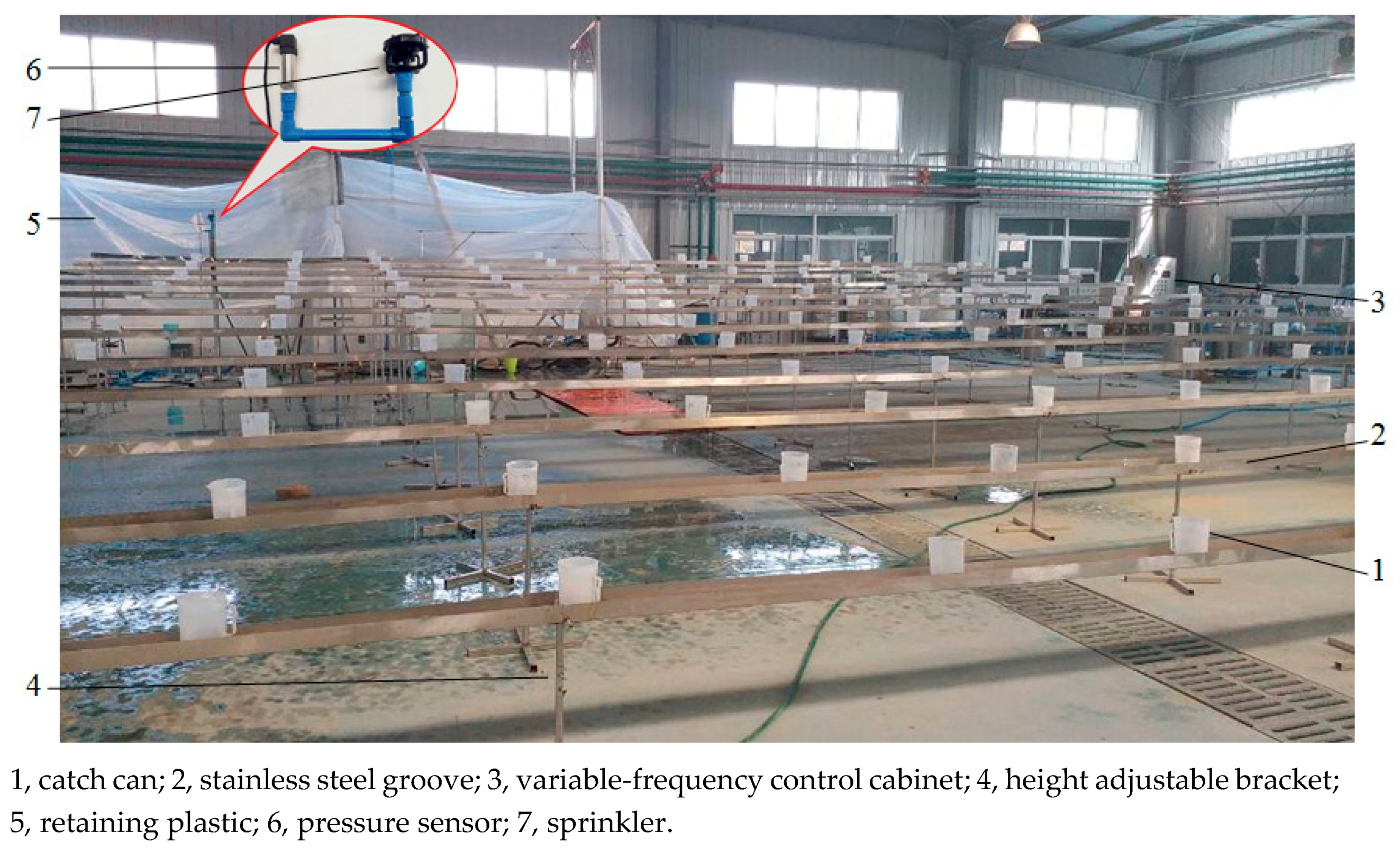
The experiment was conducted at Irrigation Hydraulics Laboratory, Northwest A&F University, Yangling, China. The experimental apparatus consisted of the automatic pressure control system, sprinkler, height adjustable bracket and the steel tank, catch-can, sprinkler screen, pressure transducer, magnetic flow rate meter, other necessary test equipment, etc., as shown in Figure 1.
The pulsating pressure was produced by an automatic pressure control system that consisted of a programmable logic controller (PLC), variable-frequency drive (VFD), and a centrifugal pump with an electric motor. The program for implementing the desired pulsating pressure was uploaded to the PLC to control the VFD, which modified the pump motor speed. The model of pulsating pressure (such as trigonometric function, sinusoidal function, trapezoidal function, etc.), the maximum pressure, the minimum pressure and the period of a function for pulsating pressure can be set in the program. Moreover, the electric motor speed of the centrifugal pump was controlled by the VFD to produce the expected pulsating pressure.
The Rainbird LF1200 sprinkler, which is very commonly used in agricultural irrigation, was selected for the study. The nozzle is 2.76 mm, elevation angle is 12°, and the recommended operating pressure range is from 210 kPa to 410 kPa for the sprinkler.
The experimental slope surface was artificially constructed by 60 height adjustable brackets and 48 steel channels with the length of 3.0 m and width of 0.15 m. There were totally 12 rows of brackets, and the length of each row was 12 m with 5 brackets in a row and 3 m bracket spacing. The horizontal distance between two rows was 1 m. The height of brackets in each row was calculated according to the experimental slope, and the actual height was adjusted according to the calculation. Four steel channels were put on each of the 5 brackets in each row to make an experimental slope surface with a length of 12 m and width of about 11 m.
Catch-cans were white plastic containers with the opening diameter of 10.6 cm and height of 14.0 cm, and they were placed in the steel tanks and arranged by grid. The grid size on the ground projection was 1 m × 1 m. There were 12 lines and 11 catch-cans on each line, and there were totally 121 catch-cans.
A sprinkler screen was constructed to prevent water from splashing on the electronic instruments. The pressure transducer was a Xi’an Xinmin model CYB, with a range from 0 to 500 kPa at ±0.1% accuracy. The pressure transducer wrapped in plastic bag was installed at the inlet of the sprinkler. The magnetic flow meter was a 25-mm Beijing Top Meter. The pressure transducer and the flow meter were connected to a data logger. The pressure and flow rate were recorded at 5-s intervals by the data logger during each 1-h sprinkler test, and then the average pressure and flow rate were calculated for each test.
For convenience of the test, the sprinkler was installed vertically at the bottom and top of the slope, respectively. The riser height was 30 cm according to the manufacturer recommendation. For the given operating pressure, the sprinkler was installed at the top of the slope firstly, and water distribution on the downhill was recorded. After the 1-h test, the sprinkler was installed at the bottom of the slope, and water distribution on the uphill was recorded under exactly the same experimental conditions. The combination of water distribution on the downhill and uphill was the water distribution on the whole slope surface.
2.2. Experimental Method
The sprinkler was tested with two different pressure models including the constant pressure and the pulsating pressure, using the same slope. The slope was 15%, which is expressed as a ratio: rise to run (increase in elevation over a horizontal distance). The constant pressure was determined as 300 kPa. The model of pulsating pressure was set as a sine wave function, and the average value of pulsating pressure was also set at 300 kPa, which was the same as the value of constant pressure. To ensure the sprinkler operated within the recommended pressure range, the maximum value of pulsating pressure was 400 kPa, and the minimum value of pulsating pressure was 200 kPa, and the period for pulsating pressure was 0.51 T0, 0.80 T0, 0.97 T0, 1.03 T0, 1.20 T0 and 1.49 T0 (“T0” means the time for sprinkler running per circle at the constant pressure of 300 kPa, and the value of “T0” here Was 17.5 s.), respectively. Hence, there were totally seven experimental trials. To obtain reliable experimental data, three replications for each trial were conducted. Each trial included two 1-h tests, that is, water distribution measured for uphill and downhill. According to International Standard (ISO15886) [15], radius of throw is the distance measured from the centerline of a continuously-operating sprinkler to the most remote point at which the sprinkler deposits water at the minimum effective water application rate (application rate equaling to or exceeding 0.26 mm/h for sprinklers with flow rates exceeding 75 L/h).The constant pressure and pulsating pressure (taking the period of 1.20 T0 as an example) measured by the pressure transducer in the experiment are shown in Figure 2.
Before water distribution measurements, relationships between pressure and flow rate were obtained for two different pressure models. To obtain these relations, the sprinkler was tested at five different constant pressures (200, 250, 300, 350 and 400 kPa) and five different pulsating pressures (average values of pulsating pressures were set at 200, 250, 300, 350 and 400 kPa, respectively; amplitudes of pulsating pressures were all 100 kPa; and periods for pulsating pressures were all 1.03 T0), and corresponding flow rates were measured. Each test duration was 1 h, during which pressure and flow rate measurements were automatically recorded every 5 s, and the average was taken.
The Christiansen Uniformity Coefficient (CU) is the most usually used indicator to assess sprinkler irrigation water application uniformity in agriculture [16,17,18]. CU can be calculated by Equation (1):
where is the measured volume from an individual catch-can; and is the average measured volume of all catch-cans. In addition, volumes can be replaced by depths in Equation (1).
Catch3D is a mathematical model that can be used to analyze the measured performance data for sprinklers in agriculture, emphasizing water application uniformity calculation [19]. It was used for some calculations of the results presented herein.
3. Results and Discussion
3.1. Sprinkler Flow Rate
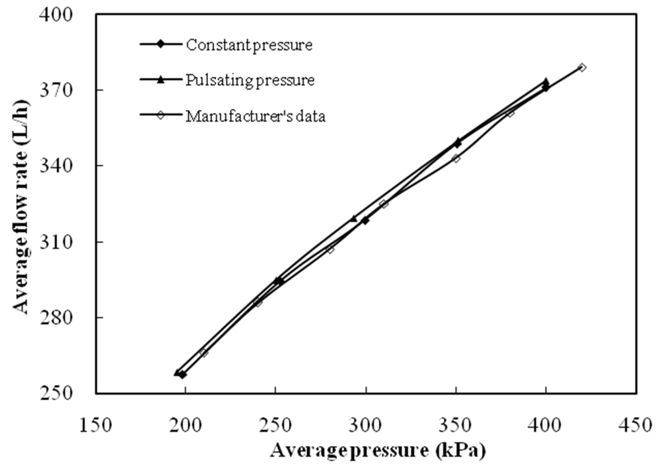
Flow rate is an important index for assessing the performance of sprinkler [20,21]. The relationship between average pressure and flow rate at the constant pressure and the pulsating pressure is shown in Figure 3. As shown in Figure 3, the pressure–discharge relation curve for the constant pressure almost coincided with that of the manufacturer’s published data, confirming that the measured flow rates are representative of a given sprinkler’s performance. In addition, the pressure–discharge relation curve for the pulsating pressure was close to that for the constant pressure. The relative difference of flow rate between the pulsating pressure and the constant pressure was within 1% at the same average pressure, indicating there was no reduction in water supply capacity for sprinkler irrigation using the pulsating pressure. Although the pulsating pressure changed as a sine wave function periodically with time, the average of pulsating pressure was the same as the constant pressure.
3.2. Sprinkler Radius of Throw
3.2.1. Measured Radius of Throw at Pulsating Pressure on Sloping Land
Radius of throw is another important index for assessing the performance of sprinkler [22,23]. The design of sprinkler spacing and lateral spacing was primarily based on radius of throw. Radii of throw are given in Table 1, where the slope is 15% and the constant pressure and the average of pulsating pressure are both 300 kPa. As shown in Table 1, the effects of period for pulsating pressure on uphill throw and downhill throw were both non-significant, because no matter on uphill or downhill, values of throw radius for different periods for pulsating pressure were very similar. Standard deviations of uphill throw and downhill throw were 0.03 m and 0.05 m, respectively. However, the pressure model had obvious influence on radius of throw. Compared with those for constant pressure, uphill and downhill throw for pulsating pressure decreased, and the magnitude of the decrease for downhill throw was larger than that for uphill throw. Uphill and downhill throw for pulsating pressure were about 0.15 m and 0.64 m shorter than those for constant pressure, respectively.
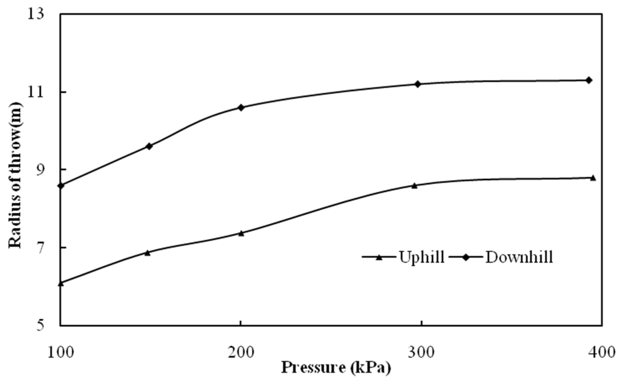
To find the reason radius of throw for pulsating pressure was shorter than that for constant pressure, the uphill throw and downhill throw on the slope of 15% at various constant pressures were measured, as shown in Figure 4. As shown in Figure 4, the uphill throw decreased from 8.75 m to 7.48 m and the magnitude of the decrease was 1.27 m when the pressure decreased from 300 kPa to 200 kPa. The uphill throw increased from 8.75 m to 9.00 m and the magnitude of the increase was only 0.25 m when the pressure increased from 300 kPa to 400 kPa. Thus, the magnitude of the uphill throw increase with increased pressure from 300 kPa to 400 kPa could not compensate the magnitude of the uphill throw decrease with decreased pressure from 300 kPa to 200 kPa. Therefore, the uphill throw for pulsating pressure was shorter than that for constant pressure of 300 kPa. The same conclusion could be reached for the downhill throw.
Additionally, it shown in Table 1, the average difference between uphill throw and downhill throw for pulsating pressure was about 0.50 m smaller than that for constant pressure. Compared with the ratio of downhill throw to uphill throw for constant pressure, the ratio for pulsating pressure decreased and the average magnitude of the decrease was about 0.056, suggesting the ratio of the wetted area on downhill to that on uphill also decreased. Theoretically, the water volume from the sprinkler to downhill was almost the same as that to uphill both for constant and pulsating pressures, not taking into account the uniformity for the sprinkler rotating speed. Thus, compared with constant pressure, the ratio of the average application rate on uphill to that on downhill reduced, which is helpful to improve the single sprinkler irrigation water application uniformity.
3.2.2. Calculated Radius of Throw at Pulsating Pressure on Sloping Land
The model of pulsating pressure used in the experiment was set as a sine wave function, which can be expressed by Equation (2):
where ti is the sprinkler running time in second; Hi is the sprinkler instantaneous operating pressure at the time ti in kPa; A is the amplitude of pulsating pressure in kPa; T is the period for pulsating pressure in second; and Ha is the average value of pulsating pressure in kPa.
According to Reference [1], uphill throw and downhill throw of rotating sprinklers at constant pressure can be estimated by Equations(3) and (4), respectively.
where Ruphill slope is the uphill throw at constant pressure in m; Rdownhill slope is the downhill throw at constant pressure in m; μ is the flow rate coefficient (the ratio of actual flow rate to ideal flow rate from nozzle), and μ = 0.86 − 0.90; H is the sprinkler operating pressure in kPa; γ is the nozzle elevation angle in degrees; β is the projected angle (the angle between the projection of water jet trajectory on slope and that on level surface) in degrees; d is the nozzle diameter in mm; and θ is the droplet landing angle on flat ground in degrees.
It is noted that Equations (3) and (4) are valid for the ground slope less than or equal to 0.20, because these equations were derived based on the hypothesis that the part of the water jet trajectory close to the horizontal plane can be approximated by a straight line when the ground slope is small.
Substituting Equation (2) into Equation (3), the instantaneous travel distance on uphill slope for water from a rotating sprinkler at the time ti can be evaluated by Equation (5):
where is the instantaneous travel distance on uphill slope for water from a rotating sprinkler at the time ti in m.
Similarly, substituting Equation (2) into Equation (4), the instantaneous travel distance on downhill slope for water from a rotating sprinkler at the time ti can be evaluated by Equation (6):
where is the instantaneous travel distance on downhill slope for water from a rotating sprinkler at the time ti in m.
Because the sprinkler operates at pulsating pressure, the sprinkler instantaneous working pressure is different when the sprinkler rotates to the same radial leg at different time. Consequently, the instantaneous travel distance for water from the sprinkler is different on the same radial leg at different time. Therefore, the effective radius of throw on the radial leg can be simply considered as an average of these instantaneous travel distances, and it can be evaluated by Equations (7) and (8).
For uphill slope:
where R’uphill slope is the uphill throw of rotating sprinklers at pulsating pressure in m; and n is times for the sprinkler rotating to the same radial leg.
For downhill slope:
where R’downhill slope is the downhill throw of rotating sprinklers at pulsating pressure in m.
When the sprinkler is selected, μ, γ and d can be known. If the model of pulsating pressure is given, A, T and Ha can be determined. β can be calculated for different sprinkler rotating angles if the slope is given [1]. θ needs to be measured on flat ground from the minimum value to maximum value of pulsating pressure before calculations of R’uphill slope and R’downhill slope. To verify the validity of Equations (7) and (8), values of θ for the Rainbird LF1200 sprinkler were measured at pressures of 200, 250, 300, 350, 400 kPa by two-dimensional video disdrometer firstly. Each measurement was repeated three times, and the average value of θ for each pressure was taken. Then, the relationship between θ and H (see Figure 5) was obtained by mathematical statistics, which can be expressed by Equation (9):
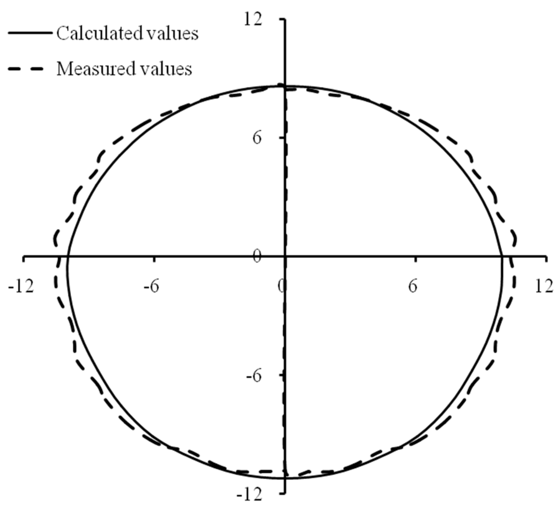
Substituting Equation (9) into Equations (7) and (8), R’uphill slope and R’downhill slope can be evaluated for the Rainbird LF1200 sprinkler at pulsating pressure on the slope of 15%. Here, the pulsating pressure was set as a sine wave function, and , and were100 kPa, 300 kPa and 18 s, respectively. The comparison of calculated and measured throw radius at pulsating pressure on sloping land is shown in Figure 6. As shown in Figure 6, most calculated values were underestimated, and the difference between calculated and measured values was within 9.33%, indicating calculated values were in good agreement with measured ones. There were three reasons for the difference between calculated and measured values. Firstly, the equation for calculating the throw radius at pulsating pressure was derived based on the hypothesis that the throw radius at pulsating pressure could be approximated by an average of water instantaneous travel distances at many constant pressures. Secondly, for convenience in the calculation of throw radius at pulsating pressure on sloping land, it was assumed that the rotation speed of sprinkler was uniform at pulsating pressure, but actually it was not. Third, the relationship between and was determined by the experimental data and methods of mathematical statistics, thus the relation was a little different from the true one. Equations (7) and (8) are helpful to determine the appropriate sprinkler spacing in the design of sprinkler irrigation used pulsating pressure on sloping land.
3.3. Water Distribution for a Single Sprinkler
Water distribution patterns for a single sprinkler at constant and pulsating pressures are shown in Figure 7, where the slope is 15%, and both the constant pressure and the average of pulsating pressure are 300 kPa, and the period for pulsating pressure is 21 s (1.20 T0). The coordinate (0, 0) in Figure 7 is the location of the sprinkler. From the aspect of water distribution shape, it is similar to an “apple-shape” for the constant pressure, and it is a little close to circular for the pulsating pressure because downhill throw decreases more obviously compared with that of constant pressure. From the aspect of water application rate, both for pulsating and constant pressures, most water fell within an area around the sprinkler. At the same distance from the sprinkler, water application rate for the pulsating pressure was generally greater than that for constant pressure, especially for downhill and positions close to the edge of wetted area. Overall, water distribution for the pulsating pressure appeared more uniform than that for the constant pressure. CU value of water distribution for a single sprinkler at pulsating pressure was 52.3%, whereas it was 42.1% at the constant pressure, about 10% lower than that of pulsating pressure. The reason was that the downhill throw for pulsating pressure was shorter than that for constant pressure, and the wetted area on downhill for pulsating pressure was smaller than that for constant pressure. According to the section of “sprinkler flow rate” depicted above, we can know that water volume from the sprinkler to downhill for pulsating pressure was almost the same as that for constant pressure, thus the average water application rate on downhill for pulsating pressure was larger than that for constant pressure, resulting in the smaller difference of average water application rate between downhill and uphill for pulsating pressure than that for constant pressure. The average water application rates on uphill and downhill for pulsating pressure were 0.89 and 0.86 mm/h, respectively, whereas they were 0.86 and 0.69 mm/h for constant pressure, respectively. Additionally, both for constant pressure and pulsating pressure, there were dark blue parts in water distributions due to the structure of the sprinkler (Figure 7). The sprinkler had four brackets connecting the inlet and cap. In the process of sprinkler rotating, water flow from the nozzle to air was affected by the four brackets, resulting in dark blue parts for water distribution.
Water distribution for pulsating pressure was more uniform than that for constant pressure, which could also be explained further by the results in Figure 8 showing the distribution frequency of water application rates (the ratio of data number for a certain range of water application rates to total number for water application rates measured by catch-can) from measured catch-can data for a single sprinkler at constant pressure and pulsating pressure. As can be seen, most water application rates were less than 1.5 mm/h for both constant pressure and pulsating pressure, covering about 85%. The average water application rates for constant pressure and pulsating pressure were 0.875 and 0.775 mm/h, respectively. However, the frequency of water application rate between 0.5 mm/h and 1.0 mm/h covered by 47.8% for the pulsating pressure, whereas 36.5% for the constant pressure, and it was 11.3% higher than that for the constant pressure. That is why the water distribution for pulsating pressure looked more uniform than that for constant pressure.
3.4. Water Distribution Overlapped and Water Application Uniformity
Rectangular arrangement is useful for overlapping water distribution and improving water application uniformity for sprinklers running on sloping land, because there is a large difference between uphill throw and downhill throw for a single sprinkler on sloping land. The overlapped water distribution for four sprinklers combination at constant pressure and pulsating pressure are shown in Figure 9, where the slope is 15%, the constant pressure and the average of pulsating pressure are both 300 kPa, the period for pulsating pressure is 21 s, and sprinkler spacing is 8 m × 10 m. Locations of the four sprinklers in Figure 9 are coordinates (0, 0), (0, 8), (10, 0) and (10, 8). As shown in Figure 9, there was a circular area with a radius of about 2 m in the middle and lower part of the overlapped rectangular area, where water application rates for pulsating pressure (3.0–4.2 mm/h) were larger than those for constant pressure (1.8–2.4 mm/h). It was mainly because, for a single sprinkler, water application rates on downhill and at the positions closed to the edge of wetted area for pulsating pressure were generally greater than those for constant pressure. Broadly, the overlapped water distribution at pulsating pressure appeared more uniform than that at constant pressure. CU values of overlapped water distribution for multiple sprinklers at pulsating pressure and constant pressure were 83.8% and 77.1%, respectively.
CU values for constant pressure and pulsating pressure with various sprinkler spacings are given in Table 2. As shown in Table 2, CU values for the pulsating pressure were on average 4.06% higher than those for the constant pressure under different spacings with sprinklers rectangular arrangement. Thus, a pulsating pressure regime could be applied in sprinkler irrigation on sloping land to improve water application uniformity. Taking irrigation quality and economy into account, a sprinkler spacing of 8–12 m is recommended for the Rainbird LF1200 sprinkler operating at pulsating pressure on slope below 15% in practice.
4. Conclusions
In this study, an experiment on water distribution under pulsating pressure and constant pressure was conducted, and the effects of pulsating pressure and constant pressure on sprinkler flow rate, radius of throw, water distribution pattern, and water application uniformity were analyzed.
The relative difference of flow rate between pulsating pressure and constant pressure was within 1% at the same average pressure, indicating there was no reduction in water supply capacity for sprinkler irrigation using pulsating pressure. Compared with constant pressure, uphill throw, downhill throw, and the ratio of downhill throw to uphill throw for pulsating pressure all decreased. From the aspect of water distribution shape, it was similar to an “apple-shape” for constant pressure, and it was a little closer to circular for pulsating pressure. From the aspect of water application rate, CU value of water distribution for a single sprinkler at pulsating pressure was 52.3%, whereas it was 42.1% at constant pressure, which was about 10% lower than that of pulsating pressure. CU data show that water distribution uniformity was improved by the pulsating pressure.
After the water distribution of single sprinkler overlapped with rectangular arrangement, CU values for pulsating pressure were on average 4.06% higher than that for constant pressure with different sprinkler spacings. Thus, a pulsating pressure regime could be applied to improve water application uniformity in sprinkler irrigation on sloping land. Taking irrigation quality and economy into account, sprinkler spacing of 8–12 m is recommended for the Rainbird LF1200 sprinkler operating at pulsating pressure on slope below 15% in practice.
Author Contributions
Investigation, N.R. and Y.H.; resources, L.Z.; data curation, B.F.; writing—original draft preparation, L.Z.; writing—review and editing, B.F.; and funding acquisition, L.Z.
Funding
This research was funded by National Natural Science Foundation of China (51779246), Key Research and Development Program of Shaanxi Province (2017NY-118), Science and Technology Program of Yangling Demonstration Zone (2017NY-28), and National Science and Technology Support Program (2015BAD22B01-02).
Conflicts of Interest
The authors declare no conflict of interest.
References
- Zhang, L.; Fu, B.Y.; Hui, X.; Ren, N.W. Simplified method for estimating throw radius of rotating sprinklers on sloping land. Irrig. Sci. 2018, 36, 329–337. [Google Scholar] [CrossRef]
- Huang, J.; Wang, J.; Zhao, X.; Wu, P.; Qi, Z.; Li, H. Effects of permanent ground cover on soil moisture in jujube orchards under sloping ground: A simulation study. Agric. Water Manag. 2014, 138, 68–77. [Google Scholar] [CrossRef]
- Wu, P.T.; Zhu, D.L.; Wang, J. Gravity-fed drip irrigation design procedure for a single-manifold subunit. Irrig. Sci. 2010, 28, 359–369. [Google Scholar] [CrossRef]
- Yu, L.; Li, N.; Liu, X.; Yang, Q.; Long, J. Influence of flushing pressure, flushing frequency and flushing time on the service life of a labyrinth-channel emitter. Biosyst. Eng. 2018, 172, 154–164. [Google Scholar] [CrossRef]
- Zhang, L.; Hui, X.; Chen, J. Effect of terrain slope on water distribution and application uniformity for sprinkler irrigation. Int. J. Agric. Biol. Eng. 2018, 11, 120–125. [Google Scholar] [CrossRef]
- Zhang, L.; Merkley, G.P.; Wu, P.; Zhu, D. Effect of catch-can spacing on calculation of sprinkler irrigation application uniformity. CLEAN Soil Air Water 2018, 46, 1800130. [Google Scholar] [CrossRef]
- Montazar, A.; Moridnejad, M. Influence of wind and bed slope on water and soil moisture distribution in solid-set sprinkler systems. Irrig. Drain. 2008, 57, 175–185. [Google Scholar] [CrossRef]
- Cisneros Espinosa, F.E.; Torres, P.; Feyen, J. Experimental Assessment of the Sprinkler Application Rate for Steep Sloping Fields. J. Irrig. Drain. Eng. 2007, 133, 276–278. [Google Scholar] [CrossRef] [Green Version]
- Keller, J.; Bliesner, R.D. Sprinkler and Trickle Irrigation; The Blackburn Press: Caldwell, NJ, USA, 2000. [Google Scholar]
- Chen, X.; Chen, D.; Yuan, D. A model for simulating application pattern of the sprinkler on sloping land. J. Hydraul. Eng. 1989, 20, 12–20. [Google Scholar]
- Li, J. Choose of suitable riser angle in sprinkler irrigation system on sloping land. J. Hydraul. Eng. 1988, 19, 45–48. [Google Scholar]
- Soares, A.A.; Willardson, L.S.; Keller, J. Surface-slope effects on sprinkler uniformity. J. Irrig. Drain. Eng. 1992, 117, 870–880. [Google Scholar] [CrossRef]
- Zhang, L.; Wu, P.; Zhu, D.; Zheng, C. Effect of pulsating pressure on labyrinth emitter clogging. Irrig. Sci. 2017, 35, 267–274. [Google Scholar] [CrossRef]
- Ge, M.; Wu, P.; Zhu, D.; Zhang, L.; Gong, X. Hydraulic performance of fixed spray plate sprinkler under dynamic water pressure. Trans. CSAM 2015, 46, 27–33. [Google Scholar]
- Agricultural Irrigation Equipment—Sprinklers—Part 3: Characterization of Distribution and Test Methods; ISO 15886-3; International Standard: Geneva, Switzerland, 2012.
- Darko, R.O.; Yuan, S.; Liu, J.; Yan, H.; Zhu, X. Overview of advances in improving uniformity and water use efficiency of sprinkler irrigation. Int. J. Agric. Biol. Eng. 2017, 10, 1–15. [Google Scholar]
- Yuan, S.; Darko, R.O.; Zhu, X.; Liu, J.; Tian, K. Optimization of movable irrigation system and performance assessment of distribution uniformity under varying conditions. Int. J. Agric. Biol. Eng. 2017, 10, 72–79. [Google Scholar]
- Zapata, N.; El Malki, E.H.; Latorre, B.; Gallinat, J.; Citoler, F.J.; Castillo, R.; Playán, E. A simulation tool for advanced design and management of collective sprinkler-irrigated areas: A study case. Irrig. Sci. 2017, 35, 327–345. [Google Scholar] [CrossRef]
- Merkley, G.P. Catch3D Users’ Guide; Civil and Environmental Engineering Department, Utah State University: Logan, UT, USA, 2004. [Google Scholar]
- O’Shaughnessy, S.A.; Andrade, M.A.; Evett, S.R. Using an integrated crop water stress index for irrigation scheduling of two corn hybrids in a semi-arid region. Irrig. Sci. 2017, 35, 451–467. [Google Scholar] [CrossRef]
- Félix-Félix, J.R.; Salinas-Tapia, H.; Bautista-Capetillo, C.; García-Aragón, J.; Burguete, J.; Playán, E. A modified particle tracking velocimetry technique to characterize sprinkler irrigation drops. Irrig. Sci. 2017, 35, 515–531. [Google Scholar] [CrossRef]
- Jiang, Y.; Li, H.; Chen, C.; Xiang, Q. Calculation and verification of formula for the range of sprinklers based on jet breakup length. Int. J. Agric. Biol. Eng. 2018, 11, 49–57. [Google Scholar] [CrossRef]
- Zhu, X.; Chikangaise, P.; Shi, W.; Chen, W.-H.; Yuan, S. Review of intelligent sprinkler irrigation technologies for remote autonomous system. Int. J. Agric. Biol. Eng. 2018, 11, 23–30. [Google Scholar] [CrossRef]
Figure 1.
Experimental setup for sprinkler water distribution on sloping ground.

Figure 2.
The measured constant pressure and pulsating pressure versus time.

Figure 3.
The relationship between flow rate and average pressure under different pressure models.

Figure 4.
Radius of throw on slope of 15% at the constant pressure.

Figure 5.
The relationship between droplet landing angle and sprinkler operating pressure.

Figure 6.
Comparison of measured and calculated values of throw radius at pulsating pressure on sloping ground. Notes: the positive and negative vertical axis represent the uphill and downhill slope direction, respectively. The horizontal and vertical axes are both in meters.
Figure 6.
Comparison of measured and calculated values of throw radius at pulsating pressure on sloping ground. Notes: the positive and negative vertical axis represent the uphill and downhill slope direction, respectively. The horizontal and vertical axes are both in meters.

Figure 7.
Water distribution for the single sprinkler.

Figure 8.
Distribution frequency of water application rates at different pressure models.

Figure 9.
Overlapped water distribution for multiple sprinklers.


Table 1.
Radius of throw at the constant pressure and the pulsating pressure.
| Pressure Model | Uphill Throw (m) | Downhill Throw (m) | Difference between Downhill Throw and Uphill Throw (m) | Ratio of Downhill Throw to Uphill Throw | |
|---|---|---|---|---|---|
| Constant Pressure | 8.75 | 11.54 | 2.79 | 1.32 | |
| Period for pulsating pressure | 0.51 T0 | 8.62 | 10.97 | 2.35 | 1.27 |
| 0.80 T0 | 8.58 | 10.83 | 2.25 | 1.26 | |
| 0.97 T0 | 8.59 | 10.93 | 2.34 | 1.27 | |
| 1.03 T0 | 8.59 | 10.91 | 2.32 | 1.27 | |
| 1.20 T0 | 8.64 | 10.89 | 2.25 | 1.26 | |
| 1.49 T0 | 8.57 | 10.89 | 2.32 | 1.27 | |
Notes: “T0” means the time for sprinkler running per circle at the constant pressure of 300 kPa. The value of “T0” here is 17.5 s.
Table 2.
Values of CU for constant and pulsating pressures with various sprinkler spacings, unit: %.
Table 2.
Values of CU for constant and pulsating pressures with various sprinkler spacings, unit: %.
| Pressure Model | Sprinkler Spacing | ||||
|---|---|---|---|---|---|
| 6 m × 8 m | 6 m × 10 m | 6 m × 12 m | 8 m × 10 m | 8 m × 12 m | |
| Constant pressure | 77.3 | 81.1 | 76.2 | 77.1 | 79.4 |
| Pulsating pressure | 78.8 | 84.1 | 82.6 | 83.8 | 82.1 |
© 2019 by the authors. Licensee MDPI, Basel, Switzerland. This article is an open access article distributed under the terms and conditions of the Creative Commons Attribution (CC BY) license (http://creativecommons.org/licenses/by/4.0/).
Share and Cite
MDPI and ACS Style
Zhang, L.; Fu, B.; Ren, N.; Huang, Y. Effect of Pulsating Pressure on Water Distribution and Application Uniformity for Sprinkler Irrigation on Sloping Land. Water 2019, 11, 913. https://doi.org/10.3390/w11050913
AMA Style
Zhang L, Fu B, Ren N, Huang Y. Effect of Pulsating Pressure on Water Distribution and Application Uniformity for Sprinkler Irrigation on Sloping Land. Water. 2019; 11(5):913. https://doi.org/10.3390/w11050913
Chicago/Turabian StyleZhang, Lin, Boyang Fu, Naiwang Ren, and Yu Huang. 2019. "Effect of Pulsating Pressure on Water Distribution and Application Uniformity for Sprinkler Irrigation on Sloping Land" Water 11, no. 5: 913. https://doi.org/10.3390/w11050913
Note that from the first issue of 2016, this journal uses article numbers instead of page numbers. See further details here.