Influences of Catchment and River Channel Characteristics on the Magnitude and Dynamics of Storage and Re-Suspension of Fine Sediments in River Beds

Abstract

Fine particles or sediments are one of the important variables that should be considered for the proper management of water quality and aquatic ecosystems. In the present study, the effect of catchment characteristics on the performance of an already developed model for the estimation of fine sediments dynamics between the water column and sediment bed was tested, using 13 catchments distributed worldwide. The model was calibrated to determine two optimal model parameters. The first is the filtration parameter, which represents the filtration of fine sediments through pores of the stream bed during the recession period of a flood event. The second parameter is the bed erosion parameter that represents the active layer, directly related to the re-suspension of fine sediments during a flood event. A dependency of the filtration parameter with the catchment area was observed in catchments smaller than ~100 km², whereas no particular relationship was observed for larger catchments (>100 km²). In contrast, the bed erosion parameter does not show a noticeable dependency with the area or other environmental characteristics. The model estimated the mass of fine sediments released from the sediment bed to the water column during flood events in the 13 catchments within ~23% bias.

1. Introduction

Fine particles or sediments are considered one of the most important factors affecting the quality and functioning of fluvial environments. For instance, fine sediments are long-lasting sources of toxic substances in catchments; that is, contaminants, such as pathogens, heavy metals as well as nutrients, are transported attached to fine sediments [1,2,3,4,5]. Fine sediment dynamics also have various effects on the health of benthic communities and the overall aquatic ecosystems [6,7,8,9].

The suspended sediment yield is affected by various catchment characteristics such as climate, geology, soils, catchment area, and land cover [10,11,12]. Because of the spatial variability of these catchment characteristics, developing a universally applicable fine sediment transport model remains an important research challenge. Rainfall intensity, erodibility and runoff processes mainly govern the fine sediment dynamics at the basin outlet. Not only these factors but also the catchment sizes cause variations in the sediment supply and transport processes. For example,

Gao et al. [13] suggested that the suspended sediment load (Q_s) is dominated by short-time-interval processes in smaller catchments with less-developed drainage density and small capacity to store fine sediment (i.e., drainage area <0.1 km²). As the drainage area increases, the homogeneity of the catchment decreases and drainage density gradually increases, leading to a greater contribution of remobilization of fine riverbed sediments and bank erosion to the overall sediment budget [13].

Suspended sediment concentration (hereafter C) is closely related to flow discharge (Q), but this relationship varies over time, from the flood scale to the annual scale. The C–Q relationship often shows orders of magnitude of scatter [14]. Such variability is explained by the fact that the rising limb of the flood generally shows a different C–Q relationship compared with the falling limb, leading to a hysteresis pattern in the relationship [13,15,16,17,18,19]. The supply of sediment from the channel system is often considered to be a significant source of sediment [18,20,21,22]. For instance, Klein [17] observed clockwise hysteresis, being mainly driven by the supply of sediments from the channel bed or from highly eroded hillslopes close to the outlet. In contrast, anticlockwise hysteresis can be observed when sediment is supplied from distant upstream sources. Recently, Yang et al. [23] derived a flow and sediment travel time model, verifying that clockwise hysteresis is observed when flow travel time is more extended than the sediment travel time, whereas anticlockwise hysteresis is observed in the opposite. More recently, Juez et al. [24], based in a series of laboratory tests, observed clockwise hysteresis driven by the supply of sediment from the channel bed, whereas anticlockwise hysteresis is observed when upstream supply of sediment has more contribution. These hysteresis patterns are one of the main reasons why single power-law models are generally insufficient to explain the scatter in the relationship between C and Q [14,25]. Seasonality of precipitation and land cover also causes scatter in C for a given Q [15,26,27,28]. For example, Alexandrov et al. [15] carried out a study in a semi-arid region and observed that autumn–spring convective storms with higher-intensity rainfall often produce higher C than winter frontal storms with lower intensity; much earlier,

Negev [26] and more recently Cantalice et al. [21] have suggested that the first flood in a given water year could have a higher C than subsequent floods of similar magnitude. The reason of these differences was attributed to the re-suspension of deposited sediment from bed during the first flood of the year. Seasonal variations of the flow due to snowmelt may also induce additional sediment supply from the channel bed and cause variations in the functional relationship between C and Q. Stubblefield et al. [29] observed an increase of the sediment supply from the channel bed when the flow rate was increased by snowmelt in a field study of Lake Tahoe. Interannual variations of the suspended sediment load with water discharge are also caused by larger-scale variations of the environment, such as climatic changes and related variability of discharge [30], or extreme events such as large floods [14].

A conceptual model coupling fine sediment dynamics with bedload transport was presented by Park and Hunt [31] based on systematic analysis of fine sediment and stream bed movement. This study led to the development of a model for the estimation of fine sediment accumulation and re-suspension from the bed [32]. It is worth mentioning that fine sediments are defined as “particles that are transported in suspension in surface waters and can also be accumulated in the sediment beds” [32]. Within this context, the objective of this study is (i) to analyze the applicability and robustness of the model developed by Park et al. [32] and (ii) to study the effect of catchment characteristics (e.g., catchment area, climate) on the performance of the model. The study was carried out based on data of 13 catchments with different drainage area and located in various hydro-climatic environments.

2. Materials and Methods

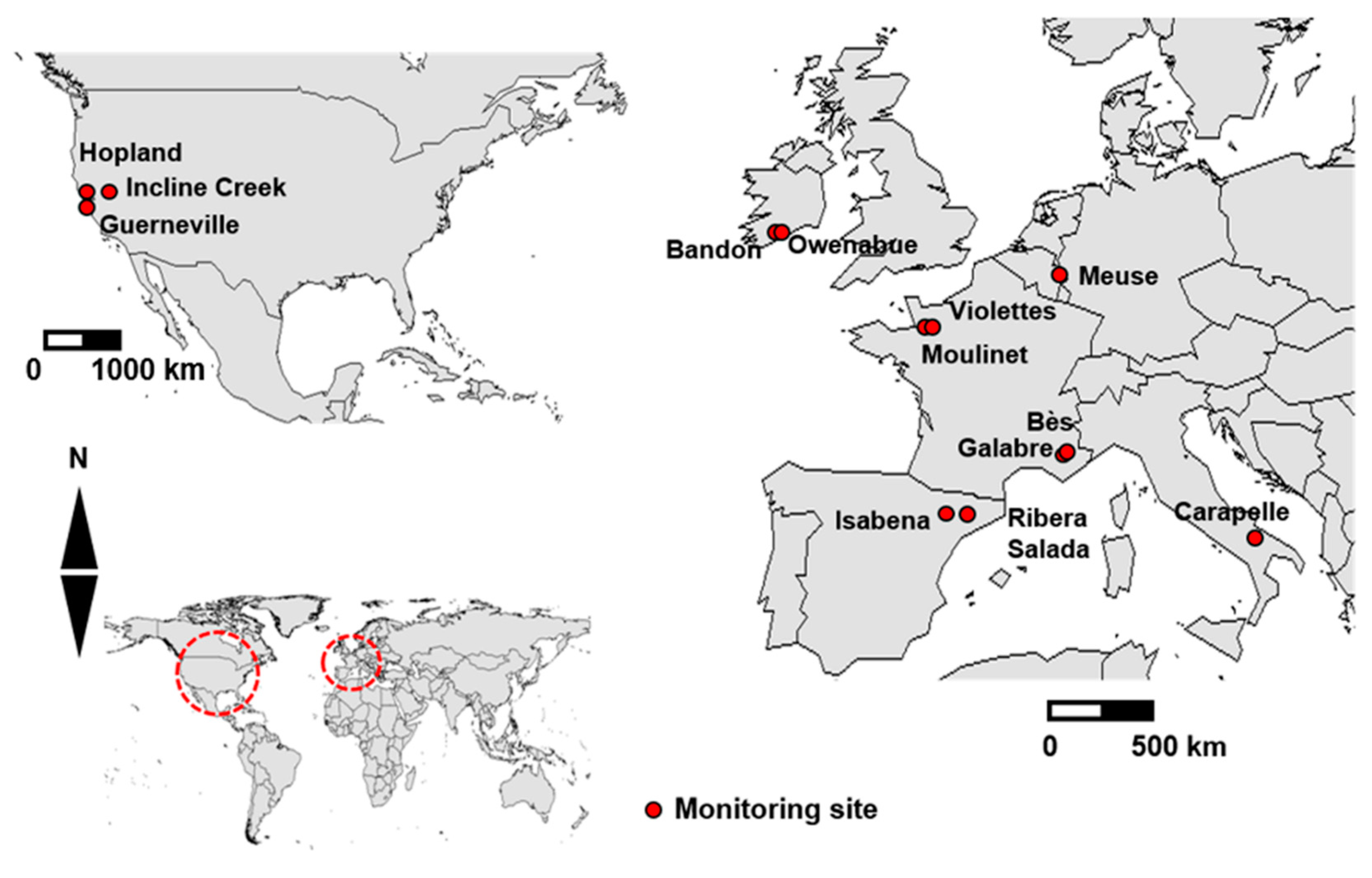
2.1. Research Sites and Data Sources

C and Q data from 13 catchments (ranging from 2.2 to 21,000 km²) were used to test the robustness of the model under different environmental characteristics (Figure 1;

Table 1. Characteristics of the studied catchments and model parameters.

No	Sites		Catchment Area (km2)	Climate	Mean Annual Precipitation (mm)	Dominant Bed Surface Materials	Observation		Qc (m3/s)	Qmax (m3/s)	Background C (Cb)	Mmax (Mg)	References
							Period	Frequency (min)
1	Violettes	France	2.2	Temperate oceanic	900	Silty loess	1 June 2002–31 May 2003	10	0.05	0.15	4000Q	6.7	[33]
2	Moulinet	France	4.5	Temperate oceanic			1 June 2002–31 May 2003	10	0.1	0.41	300Q	9.8
3	Incline Creek	Nevada, USA	7.4	Snow melt	890–1270	Sandy decomposed granite	4 April–24 May 2000	15	0.2	0.34	100(Q-0.2)	0.5	[34]
4	Galabre	France	20	Mediterranean mountainous	600–1200	Limestone and marls	3 October 2007–23December 2009	10	1	22	300Q	2200	[35]
5	Owenabue	Ireland	103	Temperate oceanic	~1200	Mudstone and sandstone	15 September 2009–15 September 2010	15	5	17	1.5Q	170	[16]
6	Bandon	Ireland	424	Temperate oceanic			10 February 2010–9 February 2011	15	10	110	0.1Q	480
7	Bès	France	165	Mediterranean mountainous	600–1200	Limestone and marls	1 April 2008–31 December 2009	10	10	143	100Q	26,600	[35]
8	Ribera Salada	Spain	114	Mediterranean mountainous	760	Limestone and conglomerates	1 November 2005–30 October 2008	5	1	5.85	10Q0.5 + 0.1Q4	53.4	[36]
9	Isabena	Spain	445	Mediterranean mountainous	770	Limestone, marls and clay-rocks	1 November 2007–30 September 2012	15	10	68	0.02Q3 + 100	100,100	[37]
10	Carapelle	Southern Italy	506	Mediterranean	450–800	clayey-loamy-sandy	1 January 2007–31 December 2011	30	8	37	5Q2	23,000	[38]
11	Hopland †	California, USA	938	Mediterranean	1000–1200	Sand-gravel and silty materials	1 October 2010–31 December 2014	15	10	425	2Q	26,560	[31,32,39]
12	Guerneville †	California, USA	3465	Mediterranean	1000–1200	Sand-gravel and silty materials	1 October 2009–31 September 2010/ 1 October 2012–31 December 2014	15	20	890	0.5Q	83,960
13	Meuse	Belgian-Dutch border	21,000	European-continental	800– 1000	Limestone, shales and sandstone	1 October 1995–30 November 2010	1440	280	1700	0.03Q	187,800	[40]

^† Data were obtained from a previous study [32].

; Table S1 in Supplementary Materials). Note that we consider environmental characteristics, as mainly, the catchment area and climatic condition of catchments.

These catchments are classified into 5 categories according to their climatic characteristics or geographical regions: (i) temperate oceanic, (ii) snowmelt, (iii) Mediterranean mountainous, (iv) Mediterranean, and (v) European-continental (Table 1).

The temperate oceanic climate is represented by two catchments located in Northwestern France, Violettes and Moulinet, where the mean longitudinal channel slope is about 1.8% in both sites [33,41]. The land in this region is used extensively for dairy cattle farming, including pastures. Cattle disturbance has been associated with bank erosion and increased suspended sediment concentration in the stream [42]. Turbidity sensors were installed at the outlet of each catchment and C was estimated from the relationship between turbidity and C [41]. The Q and C parameters were measured every 30 s, and 10-min average values were reported. Similar climatic and land use conditions are found in the Owenabue and Bandon catchments in Southern Ireland, where 90% of the land is used for pasture and tillage [16]. The Q and C values of these two catchments were provided by Ireland’s National Office of Public Works for Q and the Cork Institute of Technology for C.

Snowmelt- and glacial melt-dominated streams have periodic flow rates and corresponding fine sediment concentration fluctuations [29]. One of such streams was the Incline Creek in Nevada, which drains into Lake Tahoe, CA, USA. For this stream, Q and C were measured at 15-min intervals between 4 April and 24 May 2000. This snowmelt-dominated catchment provides an extreme test of the model, given that there are only 24 h between flood events. The gauge elevation is 2100 m a.s.l., therefore, winter precipitation falls mainly in the form of snow. The flow regime of the United States Geological Survey (USGS) station (site number 103366993) shows daily cycles reflecting snowmelt conditions in spring. The C was continuously estimated from turbidity measurements, based on the turbidity-C relationship developed by Langlois et al. [34]. The earlier arrival of suspended sediment concentration peaks compared with peak water discharge shows clockwise hysteresis loops for almost all flood events.

The Mediterranean mountainous climate was assessed in four different catchments located in two different regions. Firstly, the two tributaries of the Bléone catchment, the Galabre and Bes rivers, located in the subalpine region of southeastern France, were evaluated. The climate of the catchment is characterized by a pronounced seasonality with the occurrence of frost in winter and high-intensity rainfall in summer. The peak water discharge during the spring season is affected by snowmelt in the Bès catchment where the median grain size of bed surface materials is 70 mm [35,43]. The main types of land cover found are forests, scrubland, sparse vegetation, and grassland. Continuous Q and C values were monitored at two gauging stations located at the outlet. Depending on its magnitude, the Q was regularly gauged with the salt (NaCl) dilution method and a current flow meter. The concentration C was estimated from turbidity data based on the method developed by Navratil et al. [44].

The Ribera Salada stream, located in the southern Pyrenees, and the river Isábena (which presents frequent flooding that causes relatively high sediment transport rates) located in the southern central Pyrenees, are others representative of the Mediterranean mountainous climate. Mean annual precipitation at both catchments is around 800 mm, being the monitoring period selected for the present study representative of the long-term hydrological regime. Predominant land uses are forest in headwaters and forest mixed with agriculture at the lowlands. Q and C (estimated from turbidity sensors by establishing rating curves between turbidity and C) were continuously measured at 15-min intervals, at the Inglabaga monitoring station (channel slope at around 1%) in the case of the former [36,45], and at the Capella gauging station (channel slope at around 0.4%) for the latter, and the median grain sizes of bed surface materials are 49.0 mm and 69.5 mm in the Ribera Salada and Isábena catchments, respectively [37,46].

Another different Mediterranean environment is that of the Carapelle catchment, located in the Puglia region of Southern Italy. It presents yearly precipitation that ranges from 450 to 800 mm, and land use is mostly agricultural where the mean slope of main channel is 1.8% [38,47]. Continuous Q and C values have been measured from 1 January 2007 to 31 December 2011 in this catchment, which is characterized by long periods with low flows and a prevalence of counter-clockwise hysteresis [48]. For this reason, a shorter period, between 3 March and 31 April 2009, was utilized for calibration in this study where 2009 was quite humid year (annual rainfall 786 mm) [38,47].

The Hopland and Guerneville catchments, both located in the Russian River, California, CA, USA, analyzed in a previous study [32] were included in the catchment list; the climate in this region is also Mediterranean-type, with warmer, drier summers and cooler, wetter winters, where the median grain sizes of bed surface materials are 7.9 mm and 7.1 mm in the Hopland and Guerneville catchments, respectively.

Finally, the wet European-continental climate was considered with the inclusion of the Meuse River catchment, located at the Belgian–Dutch border, with a length of 935 km and a catchment area of 36,000 km², where wet season is between October and April, and dry season is between May and September [40]. The main channel has steep slopes and land is dominantly used for both agriculture and forest [40]. Daily Q and C data reported over 15 years by the Dutch Institute for Inland Water Management and Waste Water Treatment (RIZA) are available from the upstream of the Eijsden gauging station, where the river length is approximately 700 km and the catchment area is ~21,000 km². Because the identification of model parameters requires sufficient resolution to discern the hysteresis of C to Q in rising and falling limbs during a flood event, daily data were applicable for model simulation in this relatively large catchment.

2.2. Model Description

The model applied in this study was developed by Park et al. [32]. The model estimates in-channel storage and re-suspension of fine sediment through three phases (Phase 1–3). In the model, it is considered that the effect of other catchment characteristics, such as channel morphology, on sediment dynamics is included through two parameters. This simplicity is one of the benefits for the application of this model. The model development process will not be described in detail in this study, but the main concepts are summarized.

2.2.1. Fine Sediment Accumulation

In Phase 1, when Q is less than the critical flow rate (Q_c) to initiate sediment bed material mobilization, the fine sediments in the water column are accumulated in the sediment bed through hyporheic flow. The change of accumulated fine sediments mass during the time period from t to t + Δt is represented by Equation (1), which was derived by considering that the mass of fine sediments accumulated in the sediment bed is proportional to the fine sediment concentration in surface water, C(t).

$$\Delta \mathrm{M}\left(\mathrm{t}\right)=\mathsf{\alpha }\mathrm{C}\left(\mathrm{t}\right)\left[1-\frac{\mathrm{M}\left(\mathrm{t}\right)}{{\mathrm{M}}_{\max }}\right]\Delta \mathrm{t}\mathrm{for}\mathrm{Q}<{\mathrm{Q}}_{\mathrm{c}},$$

(1)

where $\mathrm{M}$ is the mass of fine sediments accumulated within the pore space of the sediment bed. The maximum value of M, ${\mathrm{M}}_{\max }$, represents the sediment particle accumulation capacity of the sediment bed. The sediment particle removal parameter, α (L³/T), represents the filtration and settling of fine sediment particles within the sediment bed.

2.2.2. Fine Sediment Re-Suspension

In Phase 2, during the rising flood with dQ/dt > 0 and Q > Q_c, fine sediments are released from the sediment bed into the water column, because the bed materials become fluidized when Q exceeds Q_c, initiating mobilization of the bed material.

An analysis of the data from Haschenburger [49] leads to the assumption that the erosion depth of the sediment bed during a flood event is an exponential function of the peak flow rate (Q_peak). From this approach, it is assumed that the maximum bed erosion occurs at the maximum flow rate (Q_max) during the observation period, when the release of all fine sediment particles within the sediment bed is expected. Thus M_max is observed at Q_max (Appendix A1).

In the model, the ratio of fine sediments mass released from the sediment bed, M_f,model, to the maximum possible mass of fine sediments in storage, M_max, is expressed as an exponential function of the ratio of Q_peak to Q_max. Thus, the mass of fine sediments released from the sediment bed by flood event i is

$${\mathrm{M}}_{\mathrm{fi},\mathrm{model}}={\mathrm{M}}_{\max }\exp \left[-\mathsf{\beta }\left(1-\frac{\mathrm{Q}({\mathrm{t}}_{\mathrm{p},\mathrm{i}})}{{\mathrm{Q}}_{\max }}\right)\right],$$

(2)

where ${\mathrm{t}}_{\mathrm{p},\mathrm{i}}$ is time at Q_peak of flood event i and $\mathsf{\beta }$ a dimensionless sediment bed erosion parameter.

The mass of fine sediments remaining in the pore space of the sediment bed immediately after flood event i is estimated from the difference between the accumulated fine sediment mass in the sediment bed before flood event i and the mass of fine sediments released from the sediment bed by flood event i, as

$$\mathrm{M}\left({\mathrm{t}}_{\mathrm{p},\mathrm{i}}\right)=\mathrm{M}\left({\mathrm{t}}_{\mathrm{s},\mathrm{i}}\right)-{\mathrm{M}}_{\max }\exp \left[-\mathsf{\beta }\left(1-\frac{\mathrm{Q}({\mathrm{t}}_{\mathrm{p},\mathrm{i}})}{{\mathrm{Q}}_{\max }}\right)\right],$$

(3)

where M(t) is the fine sediment mass accumulated in the sediment bed at time t, and ${\mathrm{t}}_{\mathrm{s},\mathrm{i}}$ is the time at the beginning of flood event i. In the model simulation, M(t_p,i) is restricted to be non- negative.

2.2.3. Fine Sediment Accumulation during Flood Recession

Finally, in Phase 3, in the falling limb with dQ/dt < 0 and Q > Q_c, fine sediments can be removed by filtration through hyporheic flow and stored within the pore space of the sediment bed. During flood recession, the available capacity for sediment storage is limited by partial fluidization of the sediment bed, which reduces the volume of porous media available for sediment accumulation (Appendix A2). In the model, the available capacity for sediment storage in the sediment bed during the flood recession of a flood event, M_cap, is represented as

$${\mathrm{M}}_{\mathrm{cap}}\left[\mathrm{Q}\left(\mathrm{t}\right)\right]={\mathrm{M}}_{\max }\left\{1-\exp \left[-\mathsf{\beta }\left(1-\frac{\mathrm{Q}\left(\mathrm{t}\right)}{{\mathrm{Q}}_{\max }}\right)\right]\right\},$$

(4)

The change of accumulated fine sediments mass during the flood recession period is estimated by substituting ${\mathrm{M}}_{\mathrm{cap}}\left[\mathrm{Q}\left(\mathrm{t}\right)\right]$ for ${\mathrm{M}}_{\max }$ in Equation (1) as

$$\Delta \mathrm{M}\left(\mathrm{t}\right)=\mathsf{\alpha }\mathrm{C}\left(\mathrm{t}\right)\left\{1-\frac{\mathrm{M}\left(\mathrm{t}\right)}{{\mathrm{M}}_{\mathrm{cap}}\left[\mathrm{Q}\left(\mathrm{t}\right)\right]}\right\}\Delta \mathrm{t}\mathrm{for}\mathrm{Q}>{\mathrm{Q}}_{\mathrm{c}}\mathrm{and}\mathrm{dQ}/\mathrm{dt}<0,$$

(5)

2.2.4. Model Simulation

In the model, it is assumed that M is set to M_max as an initial condition of model simulation, and remains fixed at M_max before the start of the first flood event. Then, flood event i with a flow rate exceeding Q_c erodes the mass M_f i,model, which is estimated by Equation (2), into the water column. During the flow recession, M_cap is limited below M_max, and as the flow rate recedes, M_cap increases. In the case of another flood event occurring before the flow rate recedes below Q_c, additional sediment re-suspension occurs, which also can be estimated by Equation (2). In the case that the flow rate recedes below Q_c, sediment particles can accumulate in the pore space of the sediment bed up to the maximum capacity M_max, where the accumulation rate is limited by the available mass of fine sediments in the water column. The model estimates the mass of fine sediment storage and re-suspension during the repeated cycles of flood events.

2.3. Determination of the Model Parameters

The input parameters for the model simulation are Q_c, M_max, Q_max, and background suspended sediment concentration (C_b). These parameters were determined for the 13 catchments using Equations (6)–(8) following Park et al. [32] as described below.

Park et al. [31] observed the transition in the relationship between suspended sediment load (Q_s) and Q, which occurs when the flow initiates mobilization of bed materials. The value of Q at the transition corresponds to the Q that initiates bed mobilization, defined as Q_c. The suspended sediments in the water column above the sediment bed are separated according to the source of the sediments as “background suspended sediments from the catchment (C_b)” and “fine sediments released from the sediment bed during the rising limb of a flood event”, where C_b is site-specific and represented by Equation (6):

$${\mathrm{C}}_{\mathrm{b}}\left(\mathrm{t}\right)=\mathsf{\gamma }\mathrm{Q}\left(\mathrm{t}\right),$$

(6)

in which C_b is expressed in (mg/L), Q is expressed in (m³/s), and γ is expressed in (mg·s/L/m³).

The observed mass released from the sediment bed into the water column by a flood event (M_{f, obs}) is calculated from observed data using Equation (7), whereas M_{f, model}, the modeled mass of fine sediments released from the sediment bed into the water column by a flood event, is estimated by Equation (2):

$${\mathrm{M}}_{\mathrm{fi},\mathrm{obs}}=\underset{{\mathrm{t}}_{\mathrm{s},\mathrm{i}}}{\overset{{\mathrm{t}}_{\mathrm{e},\mathrm{i}}}{{\displaystyle \int }}}\mathrm{Q}\left(\mathrm{t}\right)\left[\mathrm{C}\left(\mathrm{t}\right)-{\mathrm{C}}_{\mathrm{b}}\left(\mathrm{t}\right)\right]\mathrm{dt},$$

(7)

The lower limit of integration t_s,i is the beginning of flood event i, which is either the first occurrence when Q(t_s) > Q_c or when dQ(t)/dt transitions from negative to positive, while Q > Q_c during multiple high-flow events. The upper limit of integration t_e,i represents the time of the end of flood i, either when Q(t_e,i) < Q_c or when dQ/dt transitions from negative to positive. The maximum value of M_{f, obs} during the model calibration period is defined as M_max in the sediment bed, assuming that all fine sediments stored in the sediment bed are re-suspended during the maximum flood event when the highest peak flow rate (Q_max) is observed.

2.4. Model Evaluation

Two parameters, α and β, were utilized for model calibration. The fine sediment filtration parameter, α, represents the removal of fine sediments from the water column by filtration and settling of fine sediments within the pore space of the sediment bed of the catchment and the bed erosion parameter, β, represents the erosion of the sediment bed during a flood event. The optimal values of model parameters (α and β) were determined by a reiterative trial and error process to minimize the root-mean-square error to data standard deviation ratio (RSR), using Equations (8)–(10).

The model performance was also evaluated based on values of the term R, which is defined as the ratio of the modeled sediment mass released to the observed sediment mass released. The model performance is considered satisfactory when RSR < 0.70 [50] and when R approaches 1 when there is a total agreement between observed and predicted values.

$$\mathrm{R}=\frac{{{\displaystyle \sum }}_{\mathrm{j}=1}^{\mathrm{n}}{\mathrm{M}}_{\mathrm{fj},\mathrm{model}}}{{{\displaystyle \sum }}_{\mathrm{j}=1}^{\mathrm{n}}{\mathrm{M}}_{\mathrm{fj},\mathrm{obs}}},$$

(8)

where n is the number of flood events in the entire simulation period.

$$\mathrm{RSR}=\frac{\sqrt{{{\displaystyle \sum }}_{\mathrm{i}=1}^{\mathrm{n}}{\left({\mathrm{M}}_{\mathrm{fi},\mathrm{obs}}-{\mathrm{M}}_{\mathrm{fi},\mathrm{model}}\right)}^2}}{\sqrt{{{\displaystyle \sum }}_{\mathrm{i}=1}^{\mathrm{n}}{\left({\mathrm{M}}_{\mathrm{fi},\mathrm{obs}}-\overline{{\mathrm{M}}_{\mathrm{f},\mathrm{obs}}}\right)}^2}},$$

(9)

where n is the number of flood events and the mean observed mass released for all flood events is

$$\overline{{\mathrm{M}}_{\mathrm{f},\mathrm{obs}}}=\frac{1}{\mathrm{n}}{\displaystyle \sum }_{\mathrm{i}=1}^{\mathrm{n}}{\mathrm{M}}_{\mathrm{fi},\mathrm{obs}},$$

(10)

The period of data available for model simulation varies for each catchment. For catchments with more than three years of observations, about two-thirds of the data were used for model calibration and the remaining data were used for validation, except for the Meuse River where 15 years of data were available. Due to the longer period of observations in the Meuse River, five years were used for model calibration, whereas data from the remaining 10 years were used for model validation, in order to test the applicability of the model in a longer period.

3. Results

3.1. Model Parameters

The model parameters (i.e., Q_c, C_b, M_max, and Q_max) were determined from analysis of observed data in each of the 13 catchments (Figures S1 and S2 in Supplementary Materials) and are summarized in Table 1; a complete set of figures for all catchments is presented in Supplementary Materials, and in the next we present some observations on the data.

Slope breaks in the relationship between Q_s to Q were observed at flow rates of 5 m³/s for Owenabue and 10 m³/s for Bandon (Figure S1). The falling limb flow recessions asymptotically approached a linear relationship between C and Q, which defined the assumed background suspended sediment concentration dependence on Q as C_b(Q) = 1.5Q for Owenabue and C_b(Q) = 0.1Q for Bandon (Figure 2).

Unlike in the other catchments, the range in Q was rather small for Incline Creek; that is, 0.15 to 0.45 m³/s. In addition, the flow rates above 0.28 m³/s are reported only within a resolution of 1 cfs (cubic feet per second), thus 0.028 m³/s, which was the minimum resolution of the flow rate measurement for this USGS gauging site, leading to limited resolution of the recession curve and vertically aligned data beyond flow rates of 0.28 m³/s (Figure S1).

The relationship of Q_s to Q for water discharge above 1 m³/s for the Ribera Salada showed noticeable expansion of vertical scatter. Thus, Q_c was determined to be 1 m³/s, which corresponds to previous observations [51]. In three catchments, Ribera Salada, Isabena, and Carapelle, considerable scatter was observed in the relationship between Q_s and Q, and power laws show a reasonably good fit with the falling limb recession of flood events (Figure S2). Thus, power laws were utilized for the estimation of the background fine sediment concentrations (Table 1). The Q_c values in two subalpine regions, Galabre and Bès, were determined to be 1 m³/s and 10 m³/s, respectively (Figure S1).

The hysteresis analysis of sequential flood events provides better insight into model parameter determination. For example, much less hysteresis is observed during the second flood event of the two sequential events with similar peak flow rates between 9 and 10 August 2002, in Moulinet, France (Figure 3). This represents the depletion of stored suspended sediments by the preceding flood event and suggests that the suspended sediments were mostly supplied from the catchment during the second flood event. The observed mass of the fine sediments released from the sediment bed was 2.0 Mg for the first flood and 0.6 Mg for the second flood. The background suspended sediment concentration relationship C_b = 300 Q for Moulinet shows consistency with the suspended sediment concentration during the recession of the two flood events (Figure 3). A similar pattern of fine sediment dynamics in sequential flood events was also observed in the examples of hysteresis analysis between Q and C in other catchments. For example, much less hysteresis was observed during the second flood event of the two sequential flood events at Owenabue between 5 and 10 December 2009, at Incline Creek between 4 and 6 May 2000 and at the largest catchment Meuse between 1 December 1999 and 26 January 2000 (Figure S3). The background suspended sediment concentration relationship also shows consistency with the suspended sediment concentration during the recession of the two flood events at each site.

3.2. Model Calibration

Model calibration results are summarized in

Table 2. Model calibration results.

No	Sites	Optimal Model Parameter		Calibration			Number of Flood Events	Fine Sediment Mass
		α (m3/s)	β	RSR	R	Period		Released from Sediment Bed (Mg)	Total Mass Transported during Observation Period (Mg)	Released from Sediment Bed as Percent of Total (%)
1	Violettes	0.022	5.3	0.68	1.23	1 June 2002–31 May 2003	50	33	144	23
2	Moulinet	0.160	4.5	0.72	1.08	1 July 2002–30 June 2003	61	61	116	52
3	Incline Creek	0.25	5	0.73	0.94	4 April–24 May 2000	36	3.8	11.9	32
4	Galabre	20	2.4	0.64	1.05	3 October 2007–23 December 2009	39	14,000	26,000	54
5	Owenabue	300	4.7	0.49	0.97	15 September 2009–15 September 2010	32	1400	2500	56
6	Bandon	800	4.0	0.36	0.97	10 February 2010–9 February 2011	34	2580	3990	65
7	Bès	10	4.2	0.33	1.07	1 April 2008–31 December 2009	39	46,600	258,000	18
8	Ribera Salada	10	4.4	0.48	1.10	1 November 2005–30 October 2007	47	150	510	29
9	Isabena	10	3.9	0.97	0.93	1 November 2007–30 September 2010	79	623,000	1,063,000	58
10	Carapelle	20	3.6	0.48	0.92	3 March–23 April 2009	22	109,400	360,300	30
11	Hopland †	1000	4.4	0.36	1.02	1 October 2010–30 September 2013	69	137,000	330,000	42
12	Guerneville †	1050	4.3	0.35	0.83	1 October 2009–31 September 2010/ 1 October 2012–30 September 2013	25 (18 in 2010 water year, 8 in 2013 water year)	422,000	908,000	46
13	Meuse	1650	4.3	0.47	1.06	1 October 1995–30 September 2000	52	1,053,900	1,675,600	63

^† Data were obtained from a previous study [32].

. The model was calibrated for each catchment to determine optimal model parameters (α and β) that minimize RSR (Figure S4 in Supplementary Materials). Figure 4 shows examples of model calibrations for two catchments, Owenabue and Bandon in Ireland, where the RSR was 0.49 and 0.36, respectively. The number of flood events in each catchment ranged from 22 to 79 during the calibration period. The filtration parameter, α, ranged from 0.022 to 1650 m³/s, whereas relative consistency was observed for the bed erosion parameter, β, ranging from 2.4 to 5.3 (Figure S4 in Supplementary Materials). The model parameter sensitivity analysis shows that the model calibration stably converges to optimal values, and is more sensitive to change in α rather than β, in the two small catchments in France (Violettes and Moulinet), the snowmelt-dominated Incline Creek, and Carapelle (Figure S4). In the relatively larger catchments of Isabena, Guerneville, and Meuse, the model calibration also converges to optimal values, although it is more sensitive to change in β rather than α (Figure S4 and Park et al. [32]). In the other six catchments, Galabre, Owenabue, Bandon, Bès, Ribera Salada, and Hopland, the model calibrations are less sensitive to the change of α than to that of β when α is larger than the optimal value (Figure S4 and Park et al. [32]).

The model-estimated cumulative mass of fine sediments released from the sediment bed shows a good fit to the observations for the 13 catchments (Table 2 and Figure S5). The average RSR value in these 13 catchments is 0.54, ranging from 0.33 to 0.97, where the largest RSR of 0.97 is observed in the Isabena catchment. The model also estimated an observation bias of less than 20% in 12 catchments, except for Violettes, where R was 1.23 (Table 2).

The mass of fine sediments released from channel beds, that is, the cumulative sum of M_{f, obs}, ranged from 18% to 65% of the total suspended sediment load in the 13 catchments during the model calibration periods (Table 2), which is consistent with previous studies [52,53,54].

3.3. Model Validation

The model was applied to five catchments (Ribera Salada, Isabena, Hopland, Guerneville, and Meuse) where data for validation were available. For model validation, it was assumed that there were no observed suspended sediment data during the validation period. Thus, C_b(t) was substituted for C(t) as model input for phases 1 and 3. The number of flood events in the five catchments ranged from 10 to 101 during the validation period. The proportion of the cumulative mass of fine sediments released from the sediment bed during a flood event to total suspended load ranged from 44% to 66%. The mass was not compared in Hopland, where C data were not continuous during the validation period [32]. The validation results for each catchment are summarized in

Table 3. Model validation results.

Sites	Validation			Number of Flood Events	Fine Sediment Mass
	RSR	R	Period		Released from Sediment Bed (Mg)	Total Mass Transported during the Observation Period (Mg)	Released from Sediment Bed as Percent of Total (%)
Ribera Salada	0.71	0.98	1 November 2007–30 October 2008	52	410	930	44
Isabena	1.04	1.61	1 October 2010–30 September 2012	42	188,500	285,000	66
Hopland †	0.35	1.22	Ten flood events between 1 October 2013, and 31 December 2014	10	-	-	-
Guerneville †	0.54	0.56	1 October 2013–31 December 2014	14	224,000	366,000	61
Meuse	0.62	1.20	1 October 2000–30 November 2010	101	1,668,000	2,884,000	58

^† Data were obtained from the previous study [32].

. The average RSR and R of the five catchments were 0.65 and 1.11, respectively. The model estimated the cumulative released mass of fine sediments well, with only 2% bias, for the Ribera Salada catchment (Figure 5a). The largest RSR of 1.04 was observed in the Isabena catchment, where R was 1.61 (Figure 5b). For the Meuse River, the model showed a good fit with the observations for the 10-year validation period with 20% bias (Figure 5c). Overall, the model bias in the five catchments ranged from 2% to 61% (Table 3).

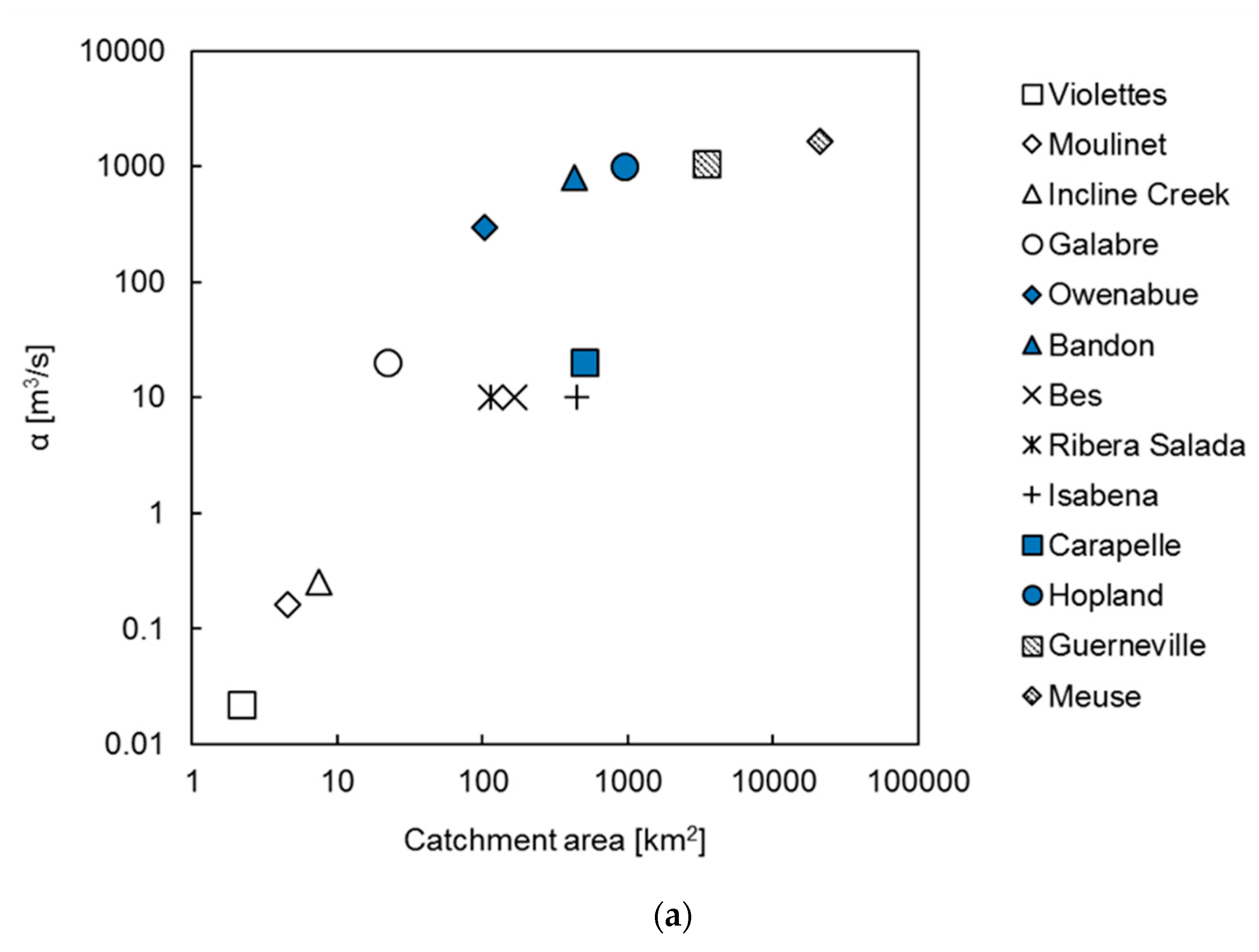
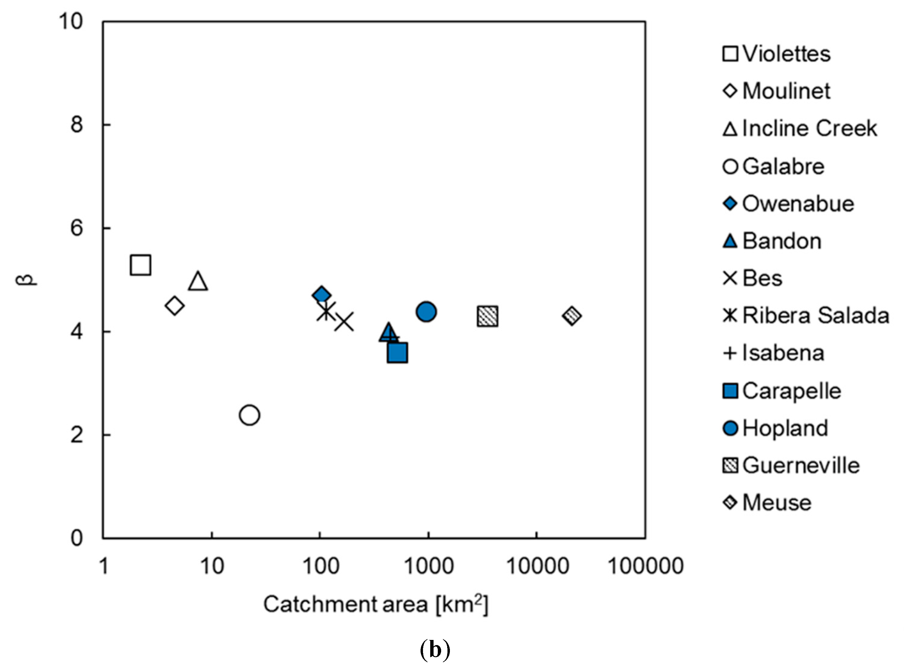
3.4. Model Parameter Dependence on Catchment Characteristics

Figure 6a plots log α against the log of the catchment area, showing that there is an increase in α with area for smaller catchments. For catchments with areas of approximately 100 km² and larger, a limited dependence on the area is observed. Although no clear dependency of α on climatic condition was observed, it is notable that similar values of α, from 10 to 20, were observed in five catchments, four (Galabre, Bès, Ribera Salada, Isabena) in Mediterranean mountainous and one (Carapelle) in Mediterranean climate, regardless of catchment area. These five catchments are located around the Mediterranean Sea with Mediterranean-type climate, where climate and bedrock show similarities (for instance, limestone is present in many areas), except for Carapelle (a clayey-loamy dominated watershed). Relatively larger values of α (>100) were observed for the five largest catchments (i.e., Owenabue, Bandon, Hopland, Guerneville, and Meuse). The catchment data that could be analyzed thus far are limited, but it is encouraging that the filtration parameter is reasonably consistent, with area dependency and with similarity between sites of similar catchment area, among a wide range of catchments. Unlike the filtration parameter (α), the bed erosion parameter (β) values varied within a narrow range of 2.4 to 5.3 in the 13 catchments without notable dependency on catchment area or other environmental characteristics (Figure 6b).

4. Discussion

The storage and re-suspension model developed by Park et al. [32] was applied to multiple catchments in contrasted climatic conditions with different catchment areas and other catchment characteristics (e.g., soil properties, and land use). Area dependency of the filtration parameter was observed, and it is notable that five catchments with Mediterranean-type climates show consistency in α, with ranges from 10 to 20 regardless of catchment scale. Relatively larger values of α (>100) were observed in larger catchments (i.e., Owenabue, Bandon, Hopland, Guerneville, and Meuse) where climatic conditions and bed material compositions were more variable (Table 1). In the case of the bed erosion parameter, the values were within a narrow range. It is clear that both α and β were affected by various environmental characteristics in each catchment. Understanding the effects of these various environmental characteristics on the model parameters, including the reason for the possible area dependency of α and relative consistency of α in the five catchments of Mediterranean-type climate, is suggested as a subject for future study.

The purpose of this study was to verify the general applicability of the storage and re-suspension model for catchments with various environmental characteristics and to understand the effect of environmental characteristics on the model performance. Therefore, providing specific values of model parameters for each catchment was out of the scope of this paper. Model calibration in 13 catchments shows a good fit with the real observations and thus verifies the possible applicability of the model, whereas there are certain areas where the applicability of the model can be improved in future studies, as described below.

(i) The first is to minimize uncertainties in determining the model input parameters Q_c, Q_max, C_b, and M_max for each catchment. Uncertainties in the determination of these model parameters can have various causes, such as limited periods of observation in the catchment and variability of sediment dynamics in the natural river system, which induce noticeable scatter of Q_s, even at the same water discharge. For example, as shown in the previous study [32], a larger peak flow rate (1050 m³/s) than Q_max (890 m³/s) was observed in Guerneville on 12 December 2014, during the validation period, which was not observed during the calibration period. The model-estimated mass of fine sediments released from the sediment bed was 72,600 Mg, which is only ~50% of the amount during the flood event [32].

In Carapelle, a Q_max of 37 m³/s and M_max of 23,000 Mg were observed on 5 March 2009, where the maximum flow rate during the model calibration period was 120 m³/s, registered on 6 March 2009. It is interesting that the flood with the largest mass of fine sediment release in Carapelle had a flow rate of only one third of the highest flow rates on record. As in Cantalice et al. [21], this could be explained by the fact that C in the first flood is related to the re-suspension of deposited sediments, whereas it decreases in the subsequent events as considerable amount of sediment was re-suspended in the previous flood event. This suggests that high rates of fine sediment erosion are possible also at moderate flow rates.

An example of model parameter uncertainty can also be drawn from the model simulation result for the Isabena. There is relatively greater disagreement between the model estimation and observations of the fine sediment mass released from the sediment bed in the Isabena, where the RSR of the model calibration is 0.97. This disagreement may be attributed to the wide range in observed suspended sediment concentrations during flood recession periods and baseflows, leading to considerable uncertainty in the assumed dependence of the background suspended sediment concentration on Q. In the Isabena, C_b was hardly discernable in the linear scale plot; thus, C_b was determined from the log–log scale (Figure S2). The wide ranges of scatter in the relationship between C and Q in the two subalpine regions, Galabre and Bès, also cause uncertainty in the determination of Q_c and C_b in the two catchments. Unlike the Isabena, even with these constraints with respect to the application of the model, the calibrated model provides good representations of the fine sediment release during flood events, with 5% and 7% bias of the observation in the two catchments, Galabre and Bès, respectively.

Overall, model calibration and validation results in this study provide a good estimation of the observed sediment dynamics. However, consistent and longer-term observations will reduce possible uncertainties, including model parameter determination, and further improve model performance.

(ii) Secondly, there are possible issues that can cause considerable model bias, such as episodic events that may produce bank erosion. For example, the model reasonably estimated the observed mass of fine sediments released from the sediment bed in Violettes (Table 2). The observed mass of fine sediments released from the sediment bed (M_{f, obs}) was less than 1 Mg when Q was less than 0.1 m³/s, except for the two flood events on 16 and 27 October 2002. The model-estimated mass of fine sediments released from the sediment bed (M_{f, model}) was less than 1 Mg for all flood events including the two events specified above, while M_{f, obs} was 3.5 Mg and 2.1 Mg, where the Q of the two flood events on 16 and 27 October was 0.09 m³/s and 0.06 m³/s, respectively. Thus, a considerable underestimation of M_{f, obs} was observed for these two flood events. This underestimation by the model may be related to the additional supply of sediment by episodic events, such as bank erosion, associated with cattle trampling in riparian pastures from March to October [33,42].

The two model parameters in this study, α and β, successfully accounted for all variability despite contrasting environmental conditions, whereas episodic events may be considered little and may increase the uncertainty of the numerical model as it was assumed that the mass of fine sediment re-suspended from the sediment bed is proportional to the bed erosion depth which is considered as an exponential function of bed shear stress. Thus, better insights into the characteristics and episodic events of each catchment would provide a better understanding of the possible reasons for the model bias and thus clues for improving the model in future studies.

Various natural characteristics can affect fine sediment dynamics, and thus should be considered for the development of sediment dynamics models for rivers. For example, in catchments with low geomorphic activity, it is possible to obtain statistically significant multivariate models to predict suspended sediment concentrations [36]. However, in catchments with greater sedimentary activity, the results of these models fail to be significant through all the time, which indicates that sediment supply and the role of the riverbed acting as a sediment source or sink play fundamental roles [55]. Riverbed sediment clogging by cohesive sediment (<63 μm) is also one of factors that have possible effect on sediment transport processes and it can be considered that in sites with sandy or sand-gravel such as the Incline Creek, the Hopland and the Guerneville, the bed material is not dominantly cohesive while the sediment is cohesive in sites with clay or silty bed material dominated such as the Violettes, the Moulinet, and the Isábena. The limitation of available information for the detailed characteristics and conditions of field sites limits the practical applicability of sediment model in many cases. Including more parameters would improve model performance but would also increase model complexity, and would require more effort for data observation and thus reduce the practical applicability of the model [32,56]. The model developed in this study includes only two model parameters, α and β, but shows good ability for estimating fine sediment storage mass in 13 catchments with various environmental characteristics, which is an obvious benefit of this model.

5. Conclusions

The general applicability of a storage and re-suspension model was tested in this study. The model was applied to 13 catchments with different climatic conditions (e.g., precipitation and hydrological conditions) and catchment area. The initial model parameters, Q_c, Q_max, C_b, and M_max, were determined from the observed data. The observed cumulative mass of fine sediments released from the bed in relation to the total suspended load during the model calibration period ranges from 18 to 65%.

The model performance was evaluated using the statistical parameters RSR and R. The optimal model simulation parameters, α and β, were determined to be values that minimize the RSR based on trial and error. The RSR of the model calibration ranges from 0.33 to 0.97, with an average value of 0.54, and the R value ranges from 0.83 to 1.23, with an average of 1.01. The value of the filtration parameter, α, ranges from 0.022 to 1650 m³/s; a clear area dependency was observed up to an approximate catchment area of less than 100 km². The bed erosion parameter, β, was set within a narrower range than α, between 2.4 and 5.3.

It is also noticeable that relatively small values of α from 10 to 20 were observed in five catchments located around the Mediterranean Sea with similar climate, while larger values of α (>100) were observed in five catchments with largest area.

Overall, the model estimated the mass of fine sediments released from the sediment bed in the 13 catchments within ~23% bias.

References

1. Droppo, I.G.; Liss, S.N.; Williams, D.; Nelson, T.; Jaskot, C.; Trapp, B. Dynamic existence of waterborne pathogens within river sediment compartments. Implications for water quality regulatory affairs. Environ. Sci. Technol. 2009, 43, 1737–1743. [Google Scholar] [CrossRef] [PubMed]
2. Søndergaard, M.; Jensen, J.P.; Jeppesen, E. Role of sediment and internal loading of phosphorus in shallow lakes. Hydrobiologia 2003, 506, 135–145. [Google Scholar] [CrossRef]
3. Singer, M.B.; Aalto, R.; James, L.A.; Kilham, N.E.; Higson, J.L.; Ghoshal, S. Enduring legacy of a toxic fan via episodic redistribution of California gold mining debris. Proc. Natl. Acad. Sci. USA 2013, 110, 18436–18441. [Google Scholar] [CrossRef]
4. Herrero, A.; Vila, J.; Eljarrat, E.; Ginebreda, A.; Sabater, S.; Batalla, R.J.; Barceló, D. Transport of sediment borne contaminants in a Mediterranean river during a high flow event. Sci. Total Environ. 2018, 633, 1392–1402. [Google Scholar] [CrossRef] [PubMed]
5. Quesada, S.; Tena, A.; Guillén, D.; Ginebreda, A.; Vericat, D.; Martínez, E.; Navarro-Ortega, A.; Batalla, R.J.; Barceló, D. Dynamics of suspended sediment borne persistent organic pollutants in a large regulated Mediterranean river (Ebro, NE Spain). Sci. Total Environ. 2014, 473, 381–390. [Google Scholar] [CrossRef] [PubMed]
6. Suttle, K.B.; Power, M.E.; Levine, J.M.; McNeely, C. How fine sediment in riverbeds impairs growth and survival of juvenile salmonids. Ecol. Appl. 2004, 14, 969–974. [Google Scholar] [CrossRef]
7. Béjar, M.; Gibbins, C.; Vericat, D.; Batalla, R.J. Effects of suspended sediment transport on invertebrate drift. River Res. Appl. 2017, 33, 1655–1666. [Google Scholar] [CrossRef]
8. Buendia, C.; Gibbins, C.N.; Vericat, D.; Batalla, R.J.; Douglas, A. Detecting the structural and functional impacts of fine sediment on stream invertebrates. Ecol. Indic. 2013, 25, 184–196. [Google Scholar] [CrossRef]
9. Buendia, C.; Gibbins, C.N.; Vericat, D.; Batalla, R.J. Effects of flow and fine sediment dynamics on the turnover of stream invertebrate assemblages. Ecohydrology 2014, 7, 1105–1123. [Google Scholar] [CrossRef]
10. Pelletier, J.D. A spatially distributed model for the long-term suspended sediment discharge and delivery ratio of drainage basins. J. Geophys. Res. 2012, 117, F2. [Google Scholar] [CrossRef]
11. Warrick, J.A.; Mertes, L.A.K. Sediment yield from the tectonically active semiarid Western Transverse Ranges of California. Geol. Soc. Am. Bull. 2009, 121, 1054–1070. [Google Scholar] [CrossRef]
12. Syvitski, J.P.; Morehead, M.D.; Bahr, D.B.; Mulder, T. Estimating fluvial sediment transport: The rating parameters. Water Resour. Res. 2000, 36, 2747–2760. [Google Scholar] [CrossRef]
13. Gao, P.; Nearing, M.A.; Commons, M. Suspended sediment transport at the instantaneous and event time scales in semiarid watersheds of southeastern Arizona, USA. Water Resour. Res. 2013, 49, 6857–6870. [Google Scholar] [CrossRef]
14. Warrick, J.A.; Madej, M.A.; Goni, M.A.; Wheatcroft, R.A. Trends in the suspended-sediment yields of coastal rivers of northern California, 1955-2010. J. Hydrol. 2013, 489, 108–123. [Google Scholar] [CrossRef]
15. Alexandrov, Y.; Laronne, J.B.; Reid, I. Intra-event and inter-seasonal behaviour of suspended sediment in flash floods of the semi-arid northern Negev, Israel. Geomorphology 2007, 85, 85–97. [Google Scholar] [CrossRef]
16. Harrington, S.T.; Harrington, J.R. An assessment of the suspended sediment rating curve approach for load estimation on the Rivers Bandon and Owenabue, Ireland. Geomorphology 2013, 185, 27–38. [Google Scholar] [CrossRef]
17. Klein, M. Anti clockwise hysteresis in suspended sediment concentration during individual storms: Holbeck catchment, Yorkshire England. Catena 1984, 11, 251–257. [Google Scholar] [CrossRef]
18. Carson, M.A.; Taylor, C.H.; Grey, B.J. Sediment production in a small Appalachian watershed during spring runoff: the Eaton Basin, 1970-1972. Can. J. Earth Sci. 1973, 10, 1707–1734. [Google Scholar] [CrossRef]
19. Williams, G.P. Sediment concentration versus water discharge during single hydrologic events in rivers. J. Hydrol. 1989, 111, 89–106. [Google Scholar] [CrossRef]
20. Harvey, J.W.; Drummond, J.D.; Martin, R.L.; McPhillips, L.E.; Packman, A.I.; Jerolmack, D.J.; Stonedahl, S.H.; Aubeneau, A.F.; Sawyer, A.H.; Larsen, L.G.; et al. Hydrogeomorphology of the hyporheic zone: Stream solute and fine particle interactions with a dynamic streambed. J. Geophys. Res. 2012, 117, G00N11. [Google Scholar] [CrossRef]
21. Cantalice, J.R.B.; Cunha, M.; Stosic, B.D.; Piscoya, V.C.; Guerra, S.M.S.; Singh, V.P. Relationship between bedload and suspended sediment in the sand-bed Exu River, in the semi-arid region of Brazil. Hydrol. Sci. J. 2013, 58, 1789–1802. [Google Scholar] [CrossRef]
22. Piqué, G.; López-Tarazón, J.A.; Batalla, R.J. Variability of in-channel sediment storage in a river draining highly erodible areas (the Isábena, Ebro Basin). J. Soil. Sediment. 2014, 14, 2031–2044. [Google Scholar] [CrossRef]
23. Yang, C.C.; Lee, K.T. Analysis of flow-sediment rating curve hysteresis based on flow and sediment travel time estimations. Int. J. Sediment Res. 2018, 33, 171–182. [Google Scholar] [CrossRef]
24. Juez, C.; Hassan, M.A.; Franca, M.J. The origin of fine sediment determines the observations of suspended sediment fluxes under unsteady flow conditions. Water Resour. Res. 2018, 54, 5654–5669. [Google Scholar] [CrossRef]
25. Walling, D.E. The sediment delivery problem. J. Hydrol. 1983, 65, 209–237. [Google Scholar] [CrossRef]
26. Negev, M. Analysis of Data on Suspended Sediment Discharge in Several Streams in Israel; Hydrological Paper No. 12; Israel Hydrological Service: Jerusalem, Israel, 1969; pp. 8–17. [Google Scholar]
27. Alexandrov, Y.; Cohen, H.; Laronne, J.B.; Reid, I. Suspended sediment load, bed load, and dissolved load yields from a semiarid drainage basin: A 15-year study. Water Resour. Res. 2009, 45, W08408. [Google Scholar] [CrossRef]
28. Brasington, J.; Richards, K. Turbidity and suspended sediment dynamics in small catchments in the Nepal Middle Hills. Hydrol. Process. 2000, 14, 2559–2574. [Google Scholar] [CrossRef]
29. Stubblefield, A.P.; Reuter, J.E.; Goldman, C.R. Sediment budget for subalpine watersheds, Lake Tahoe, California, USA. Catena 2009, 76, 163–172. [Google Scholar] [CrossRef]
30. Achite, M.; Ouillon, S. Suspended sediment transport in a semiarid watershed, Wadi Abd, Algeria (1973–1995). J. Hydrol. 2007, 343, 187–202. [Google Scholar] [CrossRef]
31. Hunt, J.R. Coupling fine particle and bedload transport in gravel-bedded streams. J. Hydrol. 2017, 552, 532–543. [Google Scholar]
32. Park, J.; Hunt, J.R. Modeling fine particle dynamics in gravel-bedded streams: Storage and re-suspension of fine particles. Sci. Total Environ. 2018, 634, 1042–1053. [Google Scholar] [CrossRef]
33. Lefrançois, J.; Grimaldi, C.; Gascuel-Odoux, C.; Gilliet, N. Suspended sediment and discharge relationships to identify bank degradation as a main sediment source on small agricultural catchments. Hydrol. Process. 2007, 21, 2923–2933. [Google Scholar] [CrossRef]
34. Langlois, J.L.; Johnson, D.W.; Mehuys, G.R. Suspended sediment dynamics associated with snowmelt runoff in a small mountain stream of Lake Tahoe (Nevada). Hydrol. Process. 2005, 19, 3569–3580. [Google Scholar] [CrossRef]
35. Navratil, O.; Evrard, O.; Esteves, M.; Legout, C.; Ayrault, S.; Némery, J.; Mate-Marin, A.; Ahmadi, M.; Lefévre, I.; Poirel, A.; Bonté, P. Temporal variability of suspended sediment sources in an alpine catchment combining river/rainfall monitoring and sediment fingerprinting. Earth Surf. Proc. Land. 2012, 37, 828–846. [Google Scholar] [CrossRef]
36. Tuset, J.; Vericat, D.; Batalla, R. Rainfall, runoff and sediment transport in a Mediterranean mountainous catchment. Sci. Total Environ. 2016, 540, 114–132. [Google Scholar] [CrossRef] [PubMed]
37. López-Tarazón, J.A.; Batalla, R.J. Dominant discharges for suspended sediment transport in a highly active Pyrenean river. J. Soil. Sediment. 2014, 14, 2019–2030. [Google Scholar] [CrossRef]
38. Gentile, F.; Bisantino, T.; Corbino, R.; Milillo, F.; Romano, G.; Trisorio Liuzzi, G. Monitoring and analysis of suspended sediment transport dynamics in the Carapelle torrent (southern Italy). Catena 2010, 80, 1–8. [Google Scholar] [CrossRef]
39. Ritter, J.R.; Brown, W.M., III. Turbidity and Suspended-Sediment Transport in the Russian River Basin; Open-File Report 72-316; United States Geological Survey: Menlo Park, CA, USA, 1971; pp. 15–29.
40. Doomen, A.; Wijma, E.; Zwolsman, J.J.; Middelkoop, H. Predicting suspended sediment concentrations in the Meuse River using a supply-based rating curve. Hydrol. Process. 2008, 22, 1846–1856. [Google Scholar] [CrossRef]
41. Birgand, F.; Lefrancois, T.; Grimaldi, C.; Novince, E.; Gilliet, N.; Odoux, C.G. Mesure des flux et échantillonnage des matières en suspension sur de petits cours déau. Ingénieries 2004, 40, 21–35. [Google Scholar]
42. Vongvixay, A.; Grimaldi, C.; Dupas, R.; Fovet, O.; Birgand, F.; Gilliet, N.; Gascuel-Odoux, C. Contrasting suspended sediment export in two small agricultural catchments: Cross-influence of hydrological behaviour and landscape degradation or stream bank management. Land Degrad. Dev. 2018, 29, 1385–1396. [Google Scholar] [CrossRef]
43. Evrard, O.; Navratil, O.; Ayrault, S.; Ahmadi, M.; Némery, J.; Legout, C.; Lefévre, I.; Poirel, A.; Bonté, P.; Esteves, M. Combining suspended sediment monitoring and fingerprinting to determine the spatial origin of fine sediment in a mountainous river catchment. Earth Surf. Proc. Land. 2011, 36, 1072–1089. [Google Scholar] [CrossRef]
44. Navratil, O.; Esteves, M.; Legout, C.; Gratiot, N.; Nemery, J.; Willmore, S.; Grangeon, T. Global uncertainty analysis of suspended sediment monitoring using turbidimeter in a small mountainous river catchment. J. Hydrol. 2011, 398, 246–259. [Google Scholar] [CrossRef]
45. Vericat, D.; Batalla, R.J.; Gibbins, C.N. Sediment entrainment and depletion from patches of fine material in a gravel-bed river. Water Resour. Res. 2008, 44, W11415. [Google Scholar] [CrossRef]
46. López-Tarazón, J.A.; Batalla, R.; Vericat, D.; Francke, T. Suspended sediment transport in a highly erodible catchment: the River Isábena (Southern Pyrenees). Geomorphology 2009, 109, 210–221. [Google Scholar] [CrossRef]
47. Bisantino, T.; Bingner, R.; Chouaib, W.; Gentile, F.; Trisorio Liuzzi, G. Estimation of runoff, peak discharge and sediment load at the event scale in a medium-size Mediterranean watershed using the AnnAGNPS model. Land Degrad. Dev. 2015, 26, 340–355. [Google Scholar] [CrossRef]
48. García-Rama, A.; Pagano, S.G.; Gentile, F.; Lenzi, M.A. Suspended sediment transport analysis in two Italian instrumented catchments. J. Mt. Sci. 2016, 13, 957–970. [Google Scholar] [CrossRef]
49. Haschenburger, J.K. A probability model of scour and fill depths in gravel-bed channels. Water Resour. Res. 1999, 35, 2857–2869. [Google Scholar] [CrossRef]
50. Moriasi, D.N.; Arnold, J.G.; Van Liew, M.W.; Bingner, R.L.; Harmel, R.D.; Veith, T.L. Model evaluation guidelines for systematic quantification of accuracy in watershed simulations. Trans. ASABE 2007, 50, 885–900. [Google Scholar] [CrossRef]
51. Vericat, D.; Batalla, R.J. Sediment transport from continuous monitoring in a perennial Mediterranean stream. Catena 2010, 82, 77–86. [Google Scholar] [CrossRef]
52. Collins, A.L.; Walling, D.E. Fine-grained bed sediment storage within the main channel systems of the Frome and Piddle catchments, Dorset, UK. Hydrol. Process. 2007, 21, 1448–1459. [Google Scholar] [CrossRef]
53. Walling, D.E.; Owens, P.N.; Leeks, G.J. The role of channel and floodplain storage in the suspended sediment budget of the River Ouse, Yorkshire, UK. Geomorphology 1998, 22, 225–242. [Google Scholar] [CrossRef]
54. Walling, D.E.; Collins, A.L.; Jones, P.A.; Leeks, G.J.L.; Old, G. Establishing fine-grained sediment budgets for the Pang and Lambourn LOCAR catchments, UK. J. Hydrol. 2006, 330, 126–141. [Google Scholar] [CrossRef]
55. López-Tarazón, J.A.; Batalla, R.J.; Vericat, D.; Balasch, J. Rainfall, runoff and sediment transport relations in a mesoscale mountainous catchment: The River Isábena (Ebro basin). Catena 2010, 82, 23–34. [Google Scholar] [CrossRef]
56. Bhosekar, A.; Ierapetritou, M. Advances in surrogate based modeling, feasibility analysis and optimization: A review. Comput. Chem. Eng. 2017, 108, 250–267. [Google Scholar] [CrossRef]
Figure 1. Location of the monitoring sites (see Table 1 and Table S1 for details of the catchments).
Water 11 00878 g001
Figure 2. Fine sediment concentration data during falling limb recession of each flood event for Owenabue from 15 September 2009, to 15 September 2010 (a), and Bandon from 10 February 2010, to 9 February 2011 (b). The symbols with different colors and shapes represent different flood events.
Water 11 00878 g002
Figure 3. (a) Hydrograph (date format: month-day hour:min) and (b) hysteresis of sediment concentration (C) to suspended sediment load (Q) for sequential floods in Moulinet between 9 and 10 August 2002.
Water 11 00878 g003
Figure 4. Model calibration output for (a) Owenabue from 15 September 2009 to 15 September 2010 and (b) Bandon from 10 February 2010 to 9 February 2011. The dashed magenta line represents the storage capacity of the sediment bed for fine sediments, Mcap [Q(t)], and the dotted black line represents the mass of the fine sediments stored in the sediment bed, M(t). The black line with triangles represents the observed cumulative mass of fine sediments released from the sediment bed by the first i flood events (Ai,obs) and the red line with circles represents the modeled cumulative mass of sediments released for the first i flood events (Ai,model).
Water 11 00878 g004
Figure 5. Model validation output for (a) the Ribera Salada from 1 November 2007 to 30 October 2008, (b) the Isabena from 1 October 2010 to 30 September 2012, and (c) the Meuse River from 1 October 2000 to 30 November 2010. The dashed magenta line represents the storage capacity of the sediment bed for fine sediments, Mcap[Q(t)], and the dotted black line represents the mass of fine sediments stored in the sediment bed, M(t). The black line with triangles represents the observed cumulative mass of fine sediments released from the sediment bed by the first i flood events (Ai,obs) and the red line with circles represents the modeled cumulative mass of sediments released for the first i flood events (Ai,model).
Water 11 00878 g005
Figure 6. Model parameter dependency on the catchment area. (a) the relationship between α and the catchment area and (b) the relationship between β and the catchment area.
Water 11 00878 g006aWater 11 00878 g006b