Causal Reasoning: Towards Dynamic Predictive Models for Runoff Temporal Behavior of High Dependence Rivers

Abstract

Nowadays, a noteworthy temporal alteration of traditional hydrological patterns is being observed, producing a higher variability and more unpredictable extreme events worldwide. This is largely due to global warming, which is generating a growing uncertainty over water system behavior, especially river runoff. Understanding these modifications is a crucial and not trivial challenge that requires new analytical strategies like Causality, addressed by Causal Reasoning. Through Causality over runoff series, the hydrological memory and its logical time-dependency structure have been dynamically/stochastically discovered and characterized. This is done in terms of the runoff dependence strength over time. This has allowed determining and quantifying two opposite temporal-fractions within runoff: Temporally Conditioned/Non-conditioned Runoff (TCR/TNCR). Finally, a successful predictive model is proposed and applied to an unregulated stretch, Mijares river catchment (Jucar river basin, Spain), with a very high time-dependency behavior. This research may have important implications over the knowledge of historical rivers´ behavior and their adaptation. Furthermore, it lays the foundations for reaching an optimum reservoir dimensioning through the building of predictive models of runoff behavior. Regarding reservoir capacity, this research would imply substantial economic/environmental savings. Also, a more sustainable management of river basins through more reliable control reservoirs’ operation is expected to be achieved.

1. Introduction

In recent decades, the alteration of traditional hydrological patterns has been increasingly more evident both worldwide and over a particular territory [1,2,3]. This is essentially materialized by more frequent and therefore less anomalous extreme events such as floods and droughts [4,5,6,7]. This is mainly due to global warming phenomenon [8,9,10], which is highly intensified by anthropogenic actions [11,12,13]. Consequently, the stationarity in hydrological time series is not strictly kept [14,15,16,17], and therefore, non-stationarity has become a common feature to deal with [18].

Not all the reasons that explain this increasing variability are brand new. Because of that, there is a consequently strong need to have powerful and reliable analytical methods to build accurate models that reproduce and forecast the future hydrological behavior of a river system [19,20,21,22,23,24,25]. Also, there is a growing necessity to design analytical strategies that allow: (a) an increase of knowledge on temporal behavior of the hydrological series [26,27], and (b) the ability to extract the logical and non-trivial time-dependency structure that underlies them [18,28,29,30].

This dual challenge, between powerful-reliable methods and new analytical strategies, is jointly addressed through the scientific approaches shown in Molina et al. [28], Zazo [30], Molina and Zazo [18,29] and Molina, et al [31], among others. This novel and active research line, focused on Causality, is characterized by increasing the knowledge of temporal behavior of water resources. This is done through the coupling among stochastic hydrological parametric models, such as Autoregressive Moving Average (ARMA) models, and innovative methodologies based on Artificial Intelligence (AI), such as Causal Reasoning (CR) supported by Bayesian modelling. In this sense, recent research suggests that this union amongst “traditional-novel approaches” provides more accurate results in the modelling of complex natural processes like hydrological behavior [22,32,33,34]. In addition, this opens new perspectives for building stochastic hydrological predictive models, able to incorporate the inherent uncertainty of the hydrological processes [29,35].

This work aims to develop a new methodological framework that will enable us to advance on the knowledge over historical adaptive behavior of river runoffs. This was addressed through Causality (Causal Reasoning, temporal dependence/independence), a powerful stochastic approach to extract the hidden logical time-dependency structure that inherently underlies into hydrological series. This approach ultimately comprises a new predictive method for the runoff temporal behavior.

In relation to previous works that integrate this research line, this paper represents a breakthrough in the characterization of the temporally runoff fractions in a high dependence rivers context. These fractions were first highlighted in Molina and Zazo [18] and referred to as Temporally Conditioned Runoff (TCR, or fraction due to time) and Non-Conditioned Runoff (TNCR, or uninfluenced by time). Now, both fractions have been determined and quantified based on dependence strength over time. Furthermore, different dynamic management scenarios (time-step by time-step) were generated according to the temporal dependence (time-lags) propagation, from which time series were obtained for each fraction. In addition, a preliminary implementation of a dynamic predictive runoff model was addressed based on the observed temporal behavior trends of both fractions in the different generated scenarios. Finally, the reliability of the predictive model was assessed from a probabilistic perspective, proposing two alternatives; the first one general and the second one detailed where the TNCR fraction adds uncertainty to the prediction because it does not depend on time.

Given that this work implies a step forward over previous ones, it is not considered appropriate to re-emphasize aspects such as the State of Art and theoretical and mathematical frameworks. To read a comprehensive and in-depth review of them, the reader is referred to the aforementioned cited works (please see [28,29,31]).

Furthermore, the application of this new analytical strategy over annual runoff series applied to reservoirs, dams, and their control operation seems quite straightforward. In this sense, the better knowledge and prediction on temporal behavior of TCR and TNCR fractions will lead to a reconsidering of the capacity of the storage reservoirs, especially convenient in the current context of global warming and for high temporal dependent river basins. This might also help for reaching an optimal dimensioning of dams, what would imply significant economic and environmental savings.

After this initial section, this work is organized as follows: a description of case study, hydrological data, and applied methodology are shown in Section 2. Section 3 provides the main experimental results from the research. In Section 4, the results are discussed in detail. Finally, Section 5 addresses the general conclusions drawn from the study.

2. Materials and Methods

2.1. Case Study

Variability and randomness are the main characteristics of water resources in Spain [29,36], which is essentially attributable to an uneven spatial and temporal distribution of the precipitations [18,37]. Indeed, the annual average rainfall in Spain presents a latitudinal decrease pattern, from wet north-west (around 2000 mm), to dry south-east with less than 200 mm [28,38]. This is aggravated by low capacity of retention of Spanish soils; on average a 9% & 34% in the rest of Europe [39].

The selected case study was Mijares river (belonging to Jucar river basin, the second largest basin on the Mediterranean side of the Iberian Peninsula). This river is situated in Eastern Spain, traditionally known as “dry Spain”. This zone regularly suffers noteworthy drought conditions [40]. In particular, an unregulated stretch, characterized by a very high time-dependency behavior and by the existence of important water springs at its headwater was selected [41] (Figure 1a). This case study was defined by gauging station “El Terde”, code number 8030 (Figure 1b).

Morphometrically, the sub-basin covers a medium-sized extension of 665 km² [42], with a main stream of 47.462 km in length, an average slope of 0.018 meter/meter. Therefore, it has a time of concentration of 12.13 h, according to Spanish regulations [43].

In lithological terms, there are important formations of loams and clays with alternation of gypsum and conglomerates or limestones and gypsums, being that these areas are generally of low permeability. However, these areas may contain deeper aquifers with greater permeability and productivity. In addition, there are small areas of limestones and dolomites where very permeable aquifers are located, generally large and productive [44].

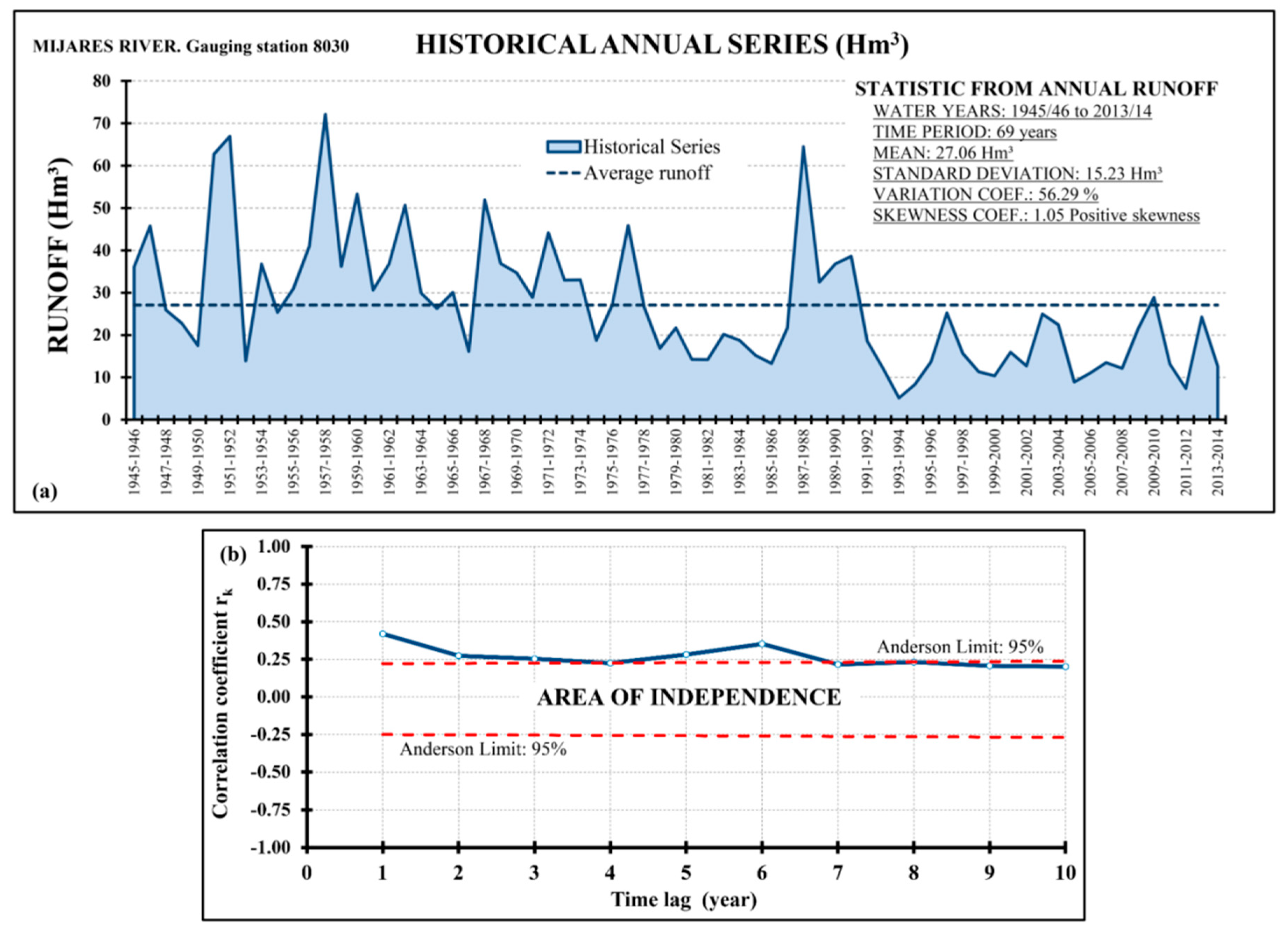
Annual runoff time series (Figure 1c) were supplied through the network of gauging stations belonging to the Jucar River Basin Authority [45]. Regarding the historical runoff, it is well known in Hydrology, at least in Spain (South Europe), that the “80 effect” which comprises a drastic reduction in Rainfall and Runoff from the year 80. In this particular basin, this effect is clearly shown in that Figure, where there is also an isolated rise for the period 1988–1991. Most of the authors and experts impute this consequence to Climate Change.

2.2. Methodololy

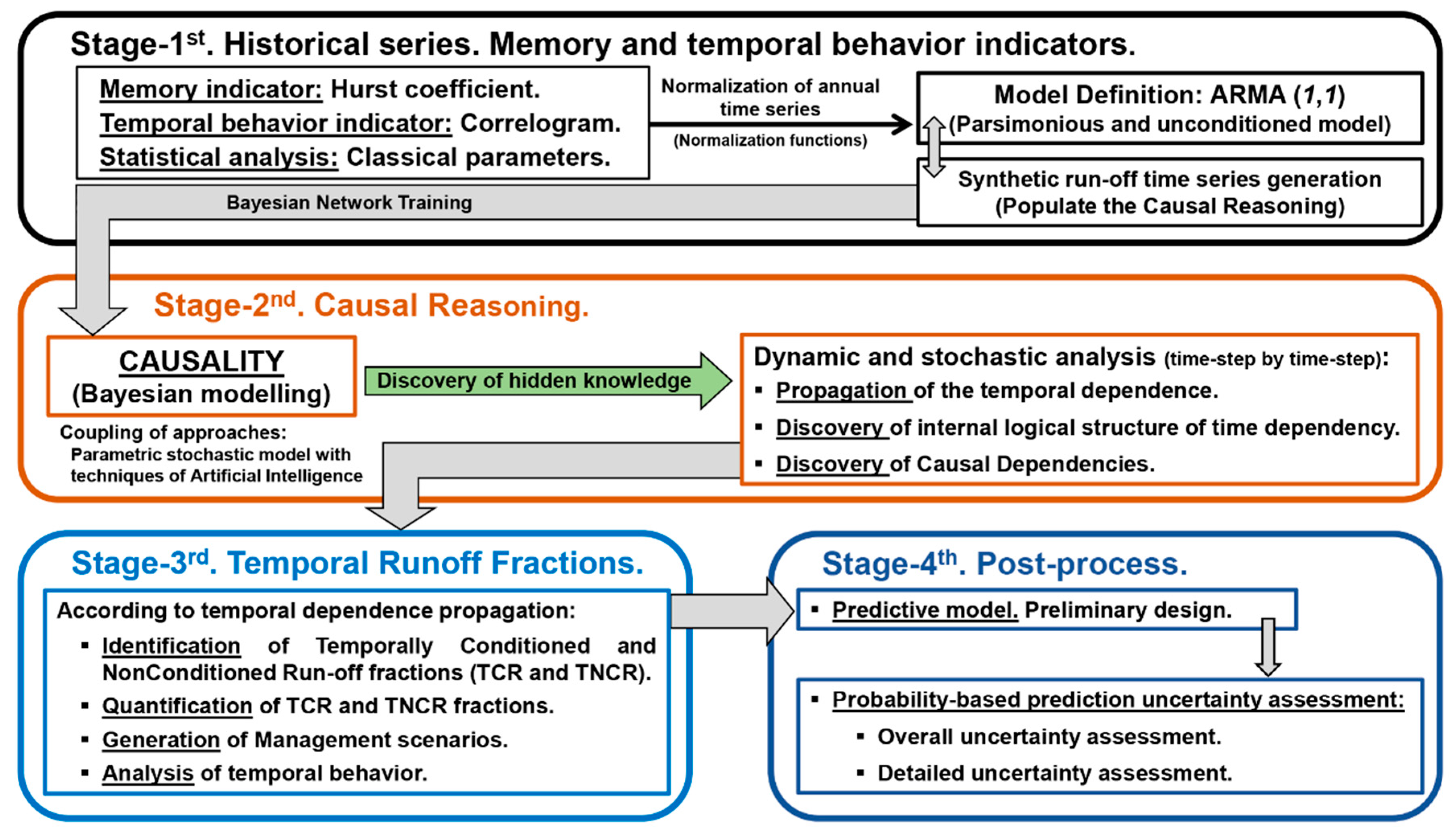
This research was articulated in four sequential stages. Firstly, in order to characterize the basin behavior, the memory and temporal behavior indicators of the historical time series were obtained, as well as its main statistical parameters. After that, equiprobable synthetic runoff series were generated through a parsimonious and unconditioned ARMA (1,1) model (Stage-1). Next, synthetic series were applied to populate the Causal Reasoning, supported by Bayesian modelling. This stage was crucial because it comprises the discovery and characterization of the logical and non-trivial time-dependency structure that inherently underlies the hydrological series (Stage-2). Then in Stage-3, based on dependence strength over the time, different dynamic management scenarios (time-step by time-step) were generated. Each temporal dependence scenario contains the dynamic and stochastic identification and quantification of the runoff temporal-fractions, TCR and TNCR. Afterward, an in-depth analysis of each of them was done. Finally, in Stage-4, a preliminary implementation of a dynamic predictive runoff model was performed and its reliability was assessed from a probabilistic perspective (Figure 2).

2.2.1. Stage-1. Historical Series. Memory and Temporal Behavior Indicators

In order to preliminarily assess the temporal nature of the basin, the memory and temporal behavior indicators of the historical time series were calculated. This was done through Hurst coefficient (H) and correlogram, respectively, based on the general framework exposed in Salas et al. [46] (pp. 41–44 and p. 49 respectively), and which are well established in the scientific community. Given that the determination of H is not a matter of this research, the reader is referred to Tyralis and Koutsoyiannis [47] where a full discussion about its accuracy is done through three different approaches. After that, main statistical parameters of the historical time series were determined. This essentially comprises getting the basic statistics parameters of the ARMA model, such as mean, standard deviation, and variation and skewness coefficients.

Secondly, a set of equiprobable synthetic runoffs were generated through a parsimonious and unconditioned ARMA (1,1) according to Molina et al. [28] and Molina and Zazo [18,29], based on the classical framework to generate ARMA models as shown by Salas et al. [46] (Chapter 5). A 20 years warm-up period was defined for achieving a “non-conditioned” synthetic series generation process without “boundary effects”.

In the context of this work, it is worth mentioning that an ARMA (p, q) model is formed by adding a moving average (MA) component to the Autoregressive (AR) component to model the temporal correlation in time series [46]. AR component (“p” part) represents the temporal dependence delay within a series; the MA component uses delays of the forecast errors to improve the process [28]. In this sense, a generic ARMA model is expressed as [48]:

$$X_t=a_t+ {\displaystyle \sum }_{j=1}^p\left({\varnothing }_{j }·X_{t-j}\right)-{\displaystyle \sum }_{j=1}^q\left({\theta }_j·a_{t-j}\right)$$

(1)

where Xt is the value of the variable at a certain time-step t, p is the number of autoregressive parameters, q is the number of moving average parameters, ${\varnothing }_j$ and ${\theta }_j$ are the coefficient of autoregressive and moving average model respectively and a_t is a random variable that represents the historical residuals (error term).

2.2.2. Stage-2. Causal Reasoning

Causality was addressed from the perspective of Causal Reasoning, which is characterized by searching reasoning patterns focused on the cause, and where the objective comprises the prediction of the effect [49]. As an analytical strategy, Bayesian modelling was selected, supported by software HUGIN Expert version 7.3 [50]. It should be noted that Bayesian modelling is a powerful AI technique based on a Probabilistic Graphical Model (PGM; [51,52,53,54]) that has significant advantages such as no need for priori information of the process and use of raw data [55,56], its usefulness for analyzing non-linear physical systems [57], or the ease of defining relationships in complex systems and offering a compact representation of the joint probability distribution over sets of random variables [21].

Causal Reasoning is carried out over a set of random decision variables called “nodes” (water years in this case), which are consecutively interconnected through “links” and a set of conditional probability tables between decision variables [21,53,54]. Furthermore, the quantification of the variables’ relationship strength is performed by Bayes’ theorem, which is propagated over time by the conditional probability; in this way the probability distributions are calculated for each decision variable as [58]:

$$P\left(A|B\right)=\frac{P\left(A,B\right)}{P\left(B\right)}=\frac{P\left(A\cap B\right)}{P\left(B\right)}$$

(2)

where P(A|B) is a probability on event A, assuming that event B is true; P(A,B) is the joint probability of events A and B; and P(B) is the probability of B.

The propagation of the Bayes’ Theorem allows, on one hand, dynamically analyze (time-step by time-step) the mitigation (evolution) of temporal dependence over time, through the relative percentage of runoff change that a time-step dynamically produces on the following ones. On the other hand, it allows for generating the yearly interactions among one target year and the previous ones through graphing of marginal dependencies in which each detected connection represents a time-dependency relationship [29].

Hydrological memory of the basin was characterized in terms of the runoff dependence strength over time. This was dynamically performed through interactions over the target year according to the time-horizon defined by the propagation of temporal dependence. The strength of each yearly interaction was evaluated by Dependence Rate (DR; from 0 to 1), expressed as [29]:

DR = 1 − (p-value)

(3)

where p-value is the measure of the strength of evidence against the independence relationship [28,30]. Therefore, a DR value equal to 1 expresses a lot of evidence of a total dependence, while in contrast 0 represents little evidence against the independence. DR values were arranged in matrix form and classified in two classes and grouped in 5 intervals (

Table 1. Dependence Rate (DR). Definition of classes and intervals.

Intervals			Classes
Range	Color Code	Description
[1.00, 0.95]		Totally dependent	DR ≥ 0.50. A lot of evidence of relevant dependencies
(0.95, 0.90]		Highly dependent
(0.90, 0.75]		Dependent
(0.75, 0.50]		Slightly dependent
(0.50, 0.00]			DR < 0.50. Little or null evidence of significant dependencies

).

This approach, based on a parsimonious and unconditioned ARMA (1,1) combined with the analytical power of Bayesian modeling, confers a high degree of freedom to the Causal Reasoning that overcoming the temporal imposition of the ARMA model [30]. This makes it possible to discover non-trivial relationships (time lag > 1) among decision variables, initially consecutively connected. In addition it allows us to discover the hidden logical time-dependency structure, which inherently underlies hydrological series [18,28,29].

For a complete definition of these processes, the reader is invited to refer to Molina et al. [28] and Molina and Zazo [29].

2.2.3. Stage-3. Temporal Runoff Fractions

Once the dependence relationships among variables and propagation of the temporal dependence were discovered through Causality, different management scenarios were dynamically/stochastically generated based on methodological framework shown in Molina and Zazo [18], and a detailed analysis of the temporal behavior was done.

In each time-step (time-lag) of the dependence propagation, both temporal-fractions, TCR (fraction due to time) and TNCR (uninfluenced by time) were determined and quantified. In this sense, the sum of both of them represents the total runoff for each water year. Both fractions are expressed as:

$$TC{R}_i=\frac{{{\displaystyle \sum }}_{j=0}^{i-1}{w}_j·Y_j}{{{\displaystyle \sum }}_{j=0}^{i-1}{w}_j},\hspace{1em}\hspace{1em}i=1, \dots , TD$$

(4)

$$TNC{R}_i=\left(R_i-TC{R}_i\right),\hspace{1em}\hspace{1em}i=1, \dots , TD$$

(5)

where $TC{R}_i$ is the weighted average conditioned runoff of the Target Year (i); $w_j$ expresses in weight form the dependence of year j on Target Year (i; please see Figure 7b); $Y_j$ is the conditioned runoff for the year j; TD is the temporal interval, expressed in years, of the propagation of dependence from lag = 0 ([0,1] when the relative percentage change is maximum) to maximum lag (when the relative percentage change is minimum and equal to zero; please see Figure 5); $R_i$ is the runoff of the time series in the target year; and $TNC{R}_i$ is the uninfluenced by time fraction for the target year.

Furthermore, in order to highlight the analytical capacity and discovery potential that this methodological framework offers for the basin water resources management, for each time-lag, two different time series were obtained, one for each temporal fraction. Next, the main statistical parameters and the coefficients of different ARMA models for each time series were determined. Consequently, the differences in the parameters and the coefficients will be exclusively due to “discovered nuances” into the temporal behavior. This was done supported by software TRASERO version 2.3.0 [48]. Akaike Information Criterion (AIC; [59]) was applied as criterion of models’ selection. This was done by maximizing the expected log-likelihood of a particular model through the maximum likelihood method. The optimal model will be the one with the lowest AIC value [60].

2.2.4. Stage-4. Post-Process.

This represents the last stage of the research. It comprises, on one side, a preliminary design of the predictive model from a probabilistic perspective, and, on the other, the assessment of the prediction reliability. The predictive model was based on the hidden temporal conditionality that inherently underlies of the historical series and that has been discovered through Causality (Stage-3).

Additionally, some studies have demonstrated the validity of stationary assumptions and stochastic parametric models applied to the generation of hydrological predictive models, such as references [61,62]. Recently, Papacharalampous et al. [61] presented an exhaustive study in which large-scale results versus traditional approaches focused on cases studies are provided. Its main conclusion is that stochastic and machine learning methods provide similar forecasts. Earlier, Tyralis and Koutsoyiannis [62] justified the validity of the stationarity hypothesis applied to stochastic methods in a context of prediction of hydroclimatic variables.

In agreement with the above conclusions, the predictive model was performed through stochastic hydrological parametric ARMA models. This was generated by parsimonious ARMA models, one for each temporal fraction (TCR and TNCR). They were developed from a time series obtained in Stage-3, according to temporal horizons of dependence mitigation.

Given that the availability of water resources in Spain is characterized by a high seasonal and annual variability [63,64,65], the predictive model was generated by a time-horizon of one (1) year (Dep-1). For that reason, the training dataset was 69 years (time period: 1945/46 to 2013/14) and the prediction was done over water year 2014/15. The obtained value of this final year was used to assess the predictive reliability based on the resulting probability.

Finally, the reliability of the predictive model was assessed from a probabilistic perspective, by suggesting two alternatives. The first one general and the second one detailed. The second approach is based on the fact that the TNCR fraction does not depend on time, and, consequently, adds uncertainty to the prediction. For that, two Monte Carlo simulations from ARMA models with 5000 data were done. The probabilistic approach was based on Gringorten probability expressed as [66]:

$$F_{\left(y_i\right)}=\frac{i-0.44}{n+0.12}$$

(6)

where $F_{\left(yi\right)}$ is the value is the value of the data distribution function $y_i$, i the occupied position by the data in the series ordered from lowest to highest, and n the total number of data in the series.

3. Results

3.1. Statistical Analysis

Figure 3 shows both the main results drawn from the traditional statistical analysis performed (Figure 3a) and the temporal correlation through correlogram (Figure 3b). Please note that the Anderson limits of a correlogram define the temporal non-dependent region; in this way, if the correlation coefficient for a certain time-lag is located inside this region, this time-step is temporally non-dependent. In addition, regarding Hurst coefficient, the resulting value was 0.84, which indicates that analyzed runoff series has a high long-term memory. This is in agreement with the observed temporal behavior shown by the correlogram. In Figure 3b it can be clearly observed that the zone of the highest dependency is mainly located in the time-lag interval [0,7].

An in-depth analysis of the correlogram reveals isolated points that may provide uncertainty on time dependence (see time-lags 4, 7 and 8). In these points, the correlation coefficient (rk) is very close to the Anderson limits, rk₄ = 0.225 [−0.257, 0.226], rk₇ = 0.216 [−0.263, 0.231] and rk₈ = 0.231 versus [−0.265, 0.232]. In addition, from rk₈ to rk₁₀ a slight trend toward an independent area of the correlogram is also observed. This is due to the average and static behavior that a correlogram offers. However, these doubts on the dependent nature of runoff series and its time-horizon will be solved by means of the dynamic analysis through the Causality.

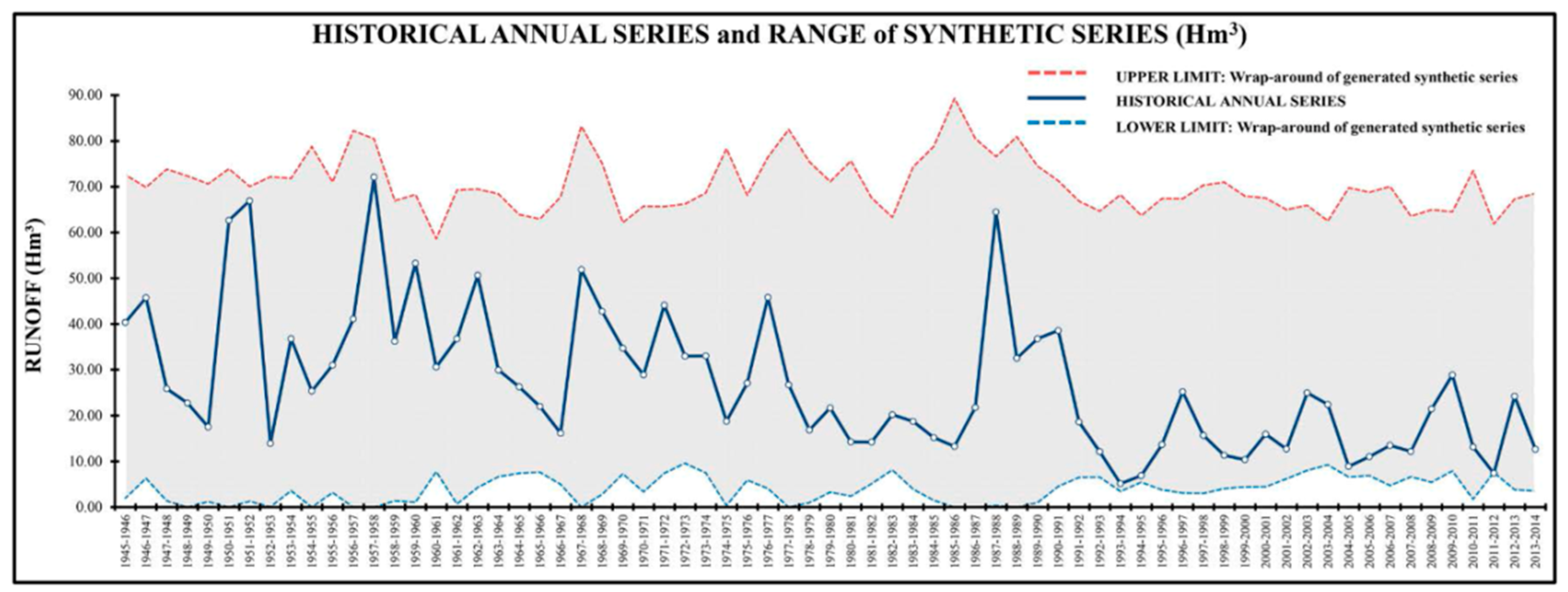
Synthetic series, obtained through a parsimonious and unconditioned ARMA (1,1) model, maintain the main statistical parameters of the runoff series (

Table 2. Main statistical parameters. Historical series versus set of synthetic series from Autoregressive Moving Average (ARMA) (1,1).

Parameters	Historical Runoff Series	Average of All Annual Synthetic Series
Mean:	27.06 Hm³	26.75 Hm³
Standard deviation:	15.23 Hm³	16.12 Hm³
Skewness coefficient 1:	1.05	1.58
Variation coefficient:	56%	59%

¹ Classic skewness coefficient.

). In this sense, Figure 4 shows the spectrum of generated synthetic series to populate and train the Causal Reasoning through Bayesian modelling.

3.2. Analysis of the Temporal Conditionality through Causal Reasoning

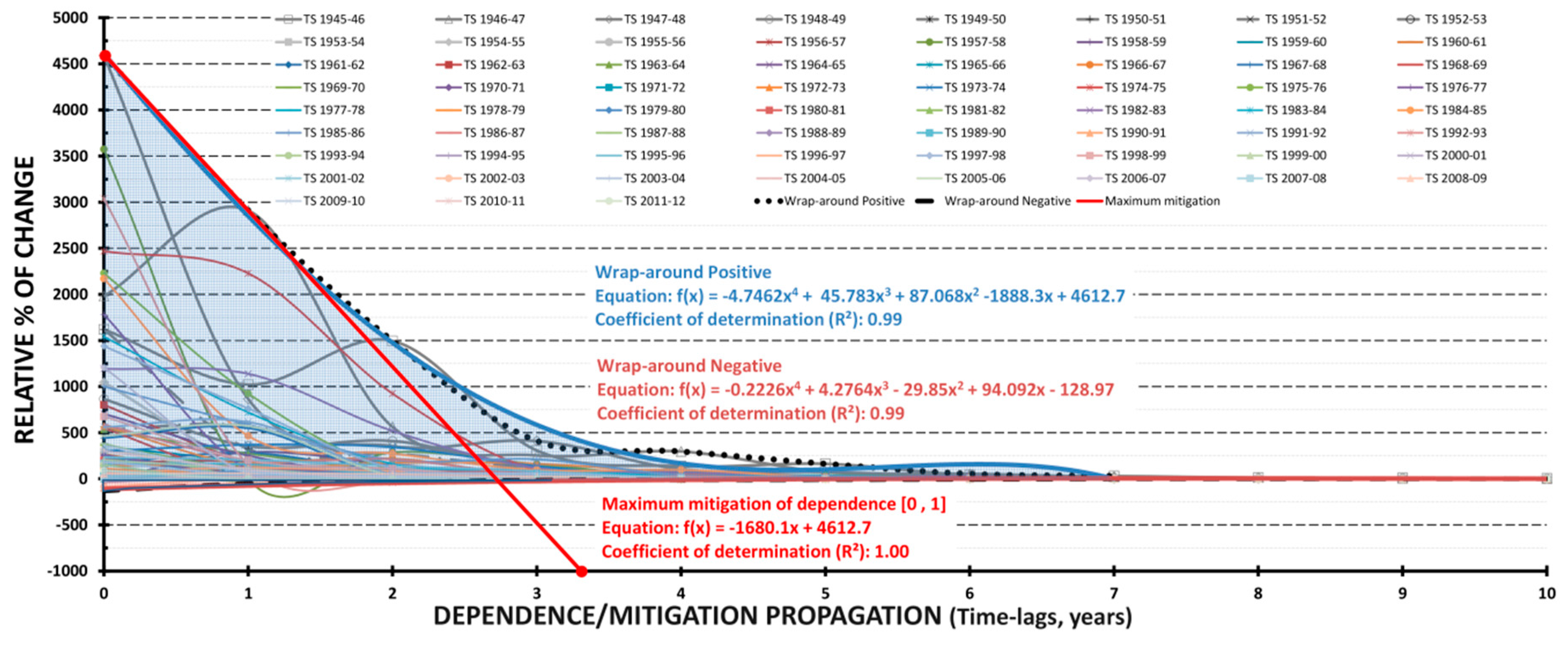
The temporal dependence propagation (mitigation) for the period 1945/46 to 2013/14 was evaluated by means of a dynamic analysis of the relative percentage of change evolution over the whole time period. Figure 5 shows the discovered dependence through the maximum (MAX or positive) and minimum (MIN or negative) wrap-around shapes and fourth-order functions, which describe the temporal behavior, these last ones with high determination coefficients (R² = 0.99 in both cases).

It is also worthy highlighting the lack of symmetry in the Figure 5, with a positive (MAX) wrap-around evidently dominant over the negative one (practically null). This reveals a clear dependence behavior which coincides with that observed in the correlogram (see Figure 3b). However, the dynamic propagation of dependence by Causal Reasoning encompasses a time-horizon of exclusively 7 years (from maximum value of relative percentage change (time-lag = 0 [0,1]) to minimum value (y-axis equal zero; time-lag = 7 [6,7]), versus 10 years shown by the average and static behavior that the correlogram offers (Figure 3b). Furthermore, uncertain points on time dependence shown in the correlogram (rk₄ and rk₇) have been eliminated by Causal Reasoning. This is shown by the dominant positive wrap-around that reveals that dependence exists but with less force. In this sense, both indeterminacies (rk₄ and rk₇) might be due to the same aforementioned reasons for the observed difference in the time horizon.

A detailed analysis of the graph of dependence propagation highlights a double dependence behavior. The first one, between interval [0,4], of greater dependence, presents a rapid mitigation of dependence from a relative percentage of change of 4,612.7 (time-lag = 0) to 167.7 (time-lag = 4), and where the maximum dependence is observed in the interval [0,1]. In contrast, the second one, in the interval [4,7] and with a reduced relevance, shows a smooth mitigation and a non-significant increase in the final interval [6,7]. These discovered, different and continuous behaviors might indicate a temporal behavior both in the short ([0,4]) and medium ([4,7]) term that is not detected by the correlogram.

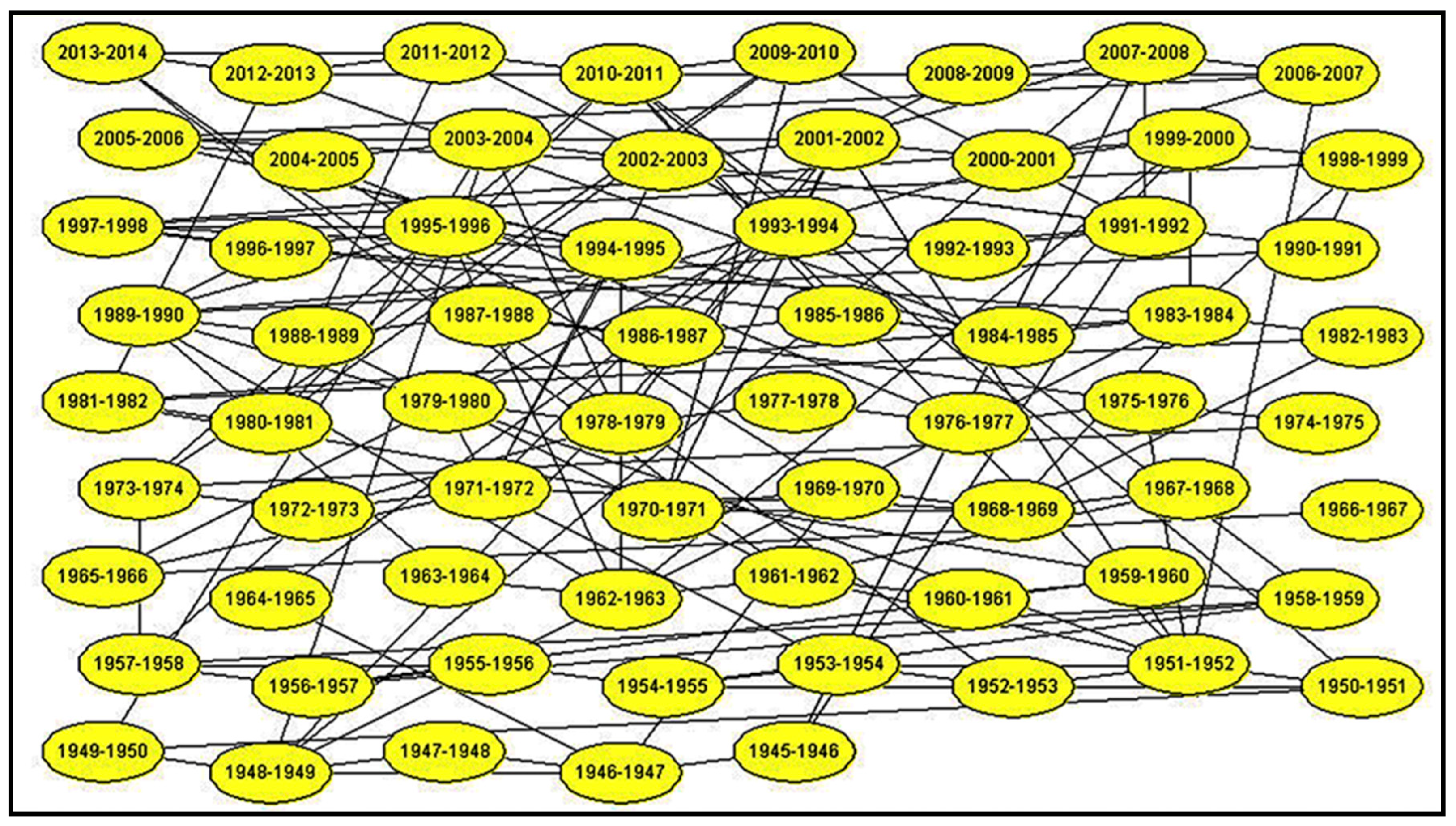
Additionally, the analytical power and suitability of Causal Reasoning applied to complex natural systems are clearly revealed in Figure 6, in which a large number of non-trivial dependency relationships (time-lag >1) amongst water years (decision variables) are revealed. Every detected connection shows an independent relationship that is measured by its p-value.

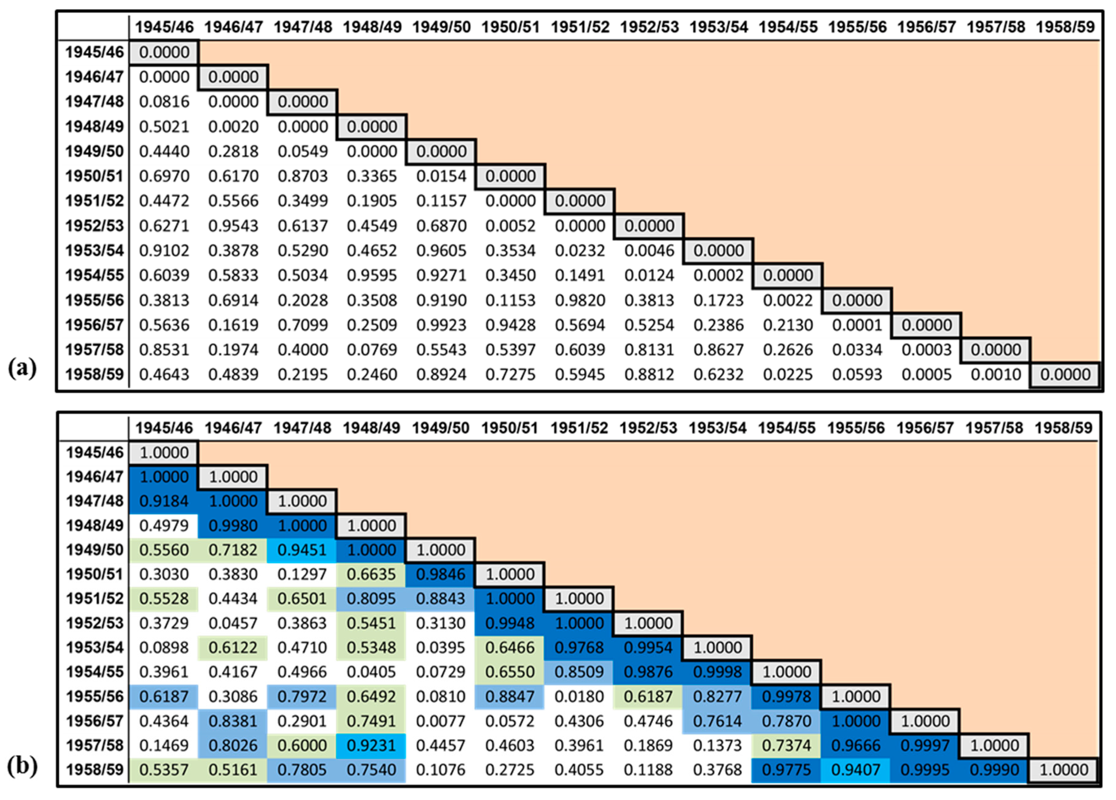
Finally, from the graph of marginal dependencies and for a 100% independence level threshold and Equation (3), Figure 7 presents, in matrix form, the hydrological memory of the basin in terms of the runoff independence/dependence strength, over time.

3.3. Management Scenarios

Applying Equations (4) and (5) over runoff series, the two temporal fractions (TCR and TNCR) were determined and quantified in agreement with the graph of mitigation/propagation of temporal dependence (see Figure 5).

Figure 8 shows the different generated dynamic management scenarios. In addition,

Table 3. Temporally Conditioned Runoff (TCR) and Temporally Non-conditioned Runoff (TNCR) Fractions. Analysis of temporal behavior for a reference threshold ².

Dependence Propagation (time-lags)	Analysis of Peaks		Analysis of Valleys		Average Behavior
	% TCR	% TNCR	% TCR	% TNCR	% TCR	% TNCR
Dependence 1 year	84.8	15.2	87.4	12.6	86.1	13.9
Dependence 2 year	78.1	21.9	76.7	23.3	77.4	22.6
Dependence 3 year	73.5	26.5	72.4	27.6	73.0	27.0
Dependence 4 year	70.1	29.9	67.2	32.8	68.7	31.3
Dependence 5 year	66.9	33.1	68.8	31.2	67.9	32.1
Dependence 6 year	65.4	34.6	67.9	32.1	66.7	33.3

² Reference threshold: Mean value of the runoff.

summarizes the evolution of both temporal fractions with respect to the mean value of runoff. In each time-lag, it can be clearly seen, as the percentages of TCR exhibit high values (always above 65% and up to mean value of 86.1%), what agrees with the Hurst coefficient (0.84). Furthermore, the dual pattern of revealed behavior by Figure 5 in two intervals [0,4] and [4,7] is also observed.

The discovery potential that this methodological framework offers for the management of the water resources of a basin is shown in the

Table 4. TCR Fraction. Evolution of the main statistical parameters according to time dependence.

Parameters	TCR Fraction
	Dependence Propagation (time-lags)
	1	2	3	4	5	6
Mean (Hm³)	23.50	21.24	20.18	19.26	18.04	17.26
Standard deviation (Hm³)	14.86	13.76	13.62	13.05	11.39	10.64
Maximum (Hm³)	72.05	70.67	70.63	69.08	66.27	62.96
Minimum (Hm³)	4.11	3.75	3.73	0.65	3.46	2.96
Range (Hm³)	67.94	66.92	66.90	68.43	62.81	60.00
Skewness coefficient 1	1.47	1.42	1.50	1.48	1.70	1.78
Variation coefficient (%)	63	65	68	68	63	62
Kurtosis	2.05	2.08	2.43	2.75	4.30	4.83

¹ Classic skewness coefficient.

and

Table 5. ARMA model selection. parameters and the coefficients.

ARMA Model (p, q)		AIC	${\varnothing }_1/{\varnothing }_2$	${\theta }_1/{\theta }_2$
Historical records	(1, 0)	−5.8705
	(1, 1)	−5.8704	0.9985	0.0007
	(1, 2)	−5.8703		0.0007/0.0007
	(2, 0)	−5.8704
	(2, 1)	−5.8703	0.9992/−0.0007	0.0001
	(2, 2)	−5.8702		0.0001/0.0007
		TCR Fraction			TNCR Fraction
		AIC	${\varnothing }_1/{\varnothing }_2$	${\theta }_1/{\theta }_2$	AIC	${\varnothing }_1/{\varnothing }_2$	${\theta }_1/{\theta }_2$
Dep-1	(1, 0)	−5.8267			−5.8469
	(1, 1)	−5.8266	0.9984	0.0007	−5.8468	0.9986	0.0007
	(1, 2)	−5.8266		0.0007/0.0007	−5.8467		0.0007/0.0007
	(2, 0)	−5.8266			−5.8468
	(2, 1)	−5.8266	0.9992/−0.0008	0.0001	−5.8467	0.9993/−0.0007	0.0001
	(2, 2)	−5.8265		0.0001/0.0007	−5.8466		0.0001/0.0007
Dep-2	(1, 0)	−5.9146			−5.4748
	(1, 1)	−5.9145	0.9985	0.0007	−5.4747	0.9979	0.0010
	(1, 2)	−5.9144		0.0007/0.0007	−5.4746		0.0010/0.0010
	(2, 0)	−5.9145			−5.4748
	(2, 1)	−5.9144	0.9993/−0.0008	−0.0001	−5.4747	0.9990/−0.0010	0.0001
	(2, 2)	−5.9143		−0.0001/0.0007	−5.4746		0.0001/0.0010
Dep-3	(1, 0)	−5.8417			−5.5094
	(1, 1)	−5.8416	0.9984	0.0007	−5.5093	0.9980	0.0010
	(1, 2)	−5.8415		0.0007/0.0007	−5.5093		0.0010/0.0010
	(2, 0)	−5.8416			−5.5093
	(2, 1)	−5.8415	0.9992/−0.0008	−0.0001	−5.5093	0.9990/−0.0010	0.0001
	(2, 2)	−5.8414		−0.0001/0.0007	−5.5092		0.0001/0.0010
Dep-4	(1, 0)	−5.8236			−5.5015
	(1, 1)	−5.8235	0.9984	0.0007	−5.5014	0.9980	0.0010
	(1, 2)	−5.8234		0.0007/0.0007	−5.5013		0.0010/0.0010
	(2, 0)	−5.8235			−5.5014
	(2, 1)	−5.8234	0.9992/−0.0008	−0.0001	−5.5013	0.9990/−0.0010	0.0001
	(2, 2)	−5.8233		−0.0001/0.0007	−5.5012		0.0001/0.0010
Dep-5	(1, 0)	−5.8776			−5.5647
	(1, 1)	−5.8776	0.9984	0.0007	−5.5646	0.9981	0.0010
	(1, 2)	−5.8776		0.0007/0.0007	−5.5645		0.0010/0.0010
	(2, 0)	−5.8776			−5.5646
	(2, 1)	−5.8776	0.9992/−0.0008	−0.0001	−5.5645	0.9990/−0.0010	0.0001
	(2, 2)	−5.8776		−0.0001/0.0007	−5.5644		0.0001/0.0010
Dep-6	(1, 0)	−5.9128			−5.5902
	(1, 1)	−5.9127	0.9985	0.0007	−5.5901	0.9981	0.0009
	(1, 2)	−5.9126		0.0007/0.0007	−5.5900		0.0009/0.0009
	(2, 0)	−5.9127			−5.5901
	(2, 1)	−5.9126	0.9992/−0.0008	−0.0001	−5.5900	0.9991/−0.0009	0.0001
	(2, 2)	−5.9125		−0.0001/0.0007	−5.5899		0.0001/0.0009

.

Regarding the ARMA models coefficients of the TCR fraction, their range does not show a significant variability. However, slight nuances are evident in their behavior because of the propagation of time dependence. Classical analysis does not detect this because the coefficients are unique and fixed in each model. In contrast, the TNCR fraction variability is greater, especially in the ${\varnothing }_1$ coefficient (from 0.9979 to 0.9993) versus the fixed coefficients of the historical series (0.9985 and 0.9992). This would allow for a better characterization of this uninfluenced by time fraction, and therefore, the uncertainty of temporal behavior would be reduced.

3.4. Predictive Model. Probability-Based Assessment

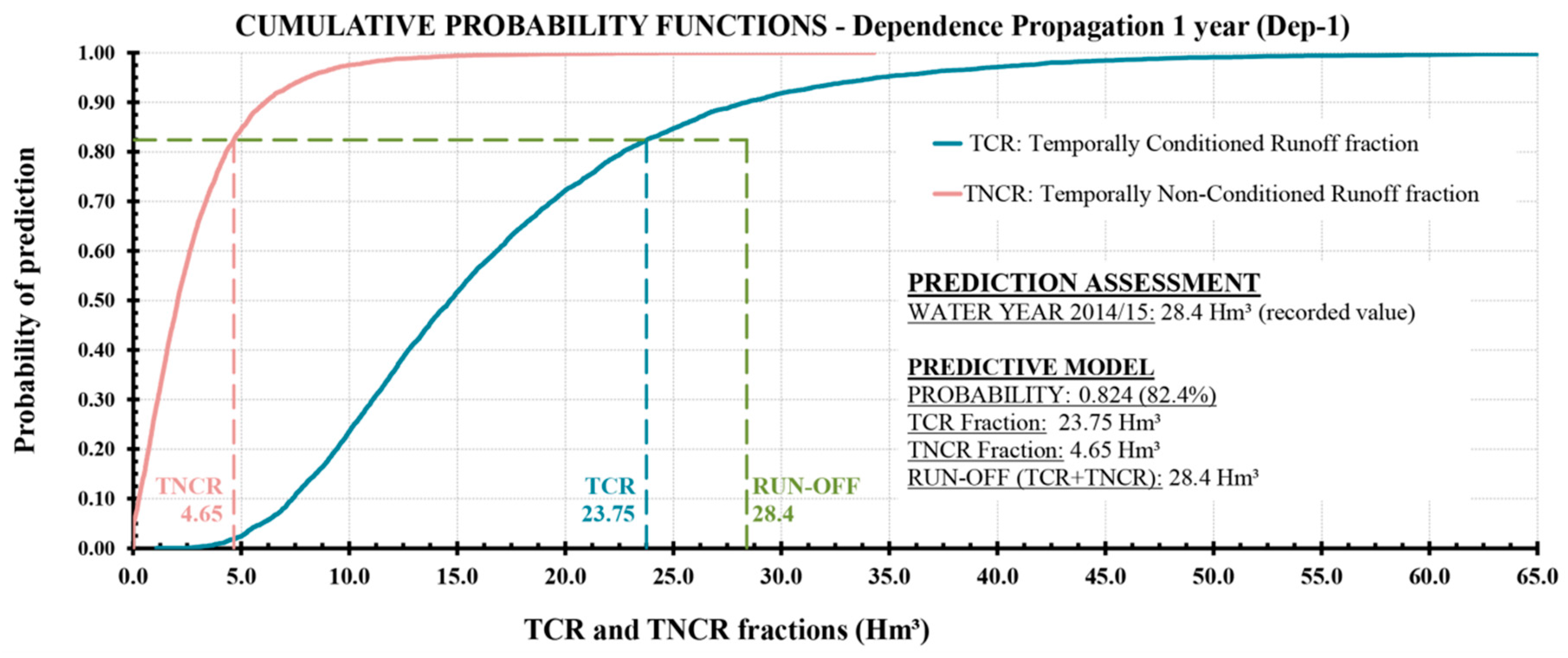
Figure 9 shows the design of the dynamic predictive model over the time-horizon of one (1) year (target water year 2014/15). This was performed by means of the conditioned data (Table 3), TCR and TNCR fractions time series for a one-year time dependency (Dep-1; Figure 8) and two parsimonious ARMA (1,0) models, defined each of them over those runoff temporal-fractions. It should be noted that model selection was carried out by Akaike Information Criterion, due to AIC of the ARMA models from (1.0) to (2.2) reported a slight difference in each one of the fractions (TCR: [−5.8267, −5.8265]; TNCR [−5.8469, −5.8466]; see Table 5).

On the other hand, the reliability of the predictive model is shown in

Table 6. Prediction Analysis for a Dependence Propagation one year (Dep-1).

Probability	TCR	TNCR 3	Runoff Prediction
			Overall	Detailed
0.50	14.68	2.06	16.74	14.68 ± 2.06	[12.62, 16.74]
0.60	16.82	2.62	19.44	16.82 ± 2.62	[14.20, 19.44]
0.70	19.38	3.37	22.75	19.38 ± 3.37	[16.01, 22.75]
0.80	22.67	4.30	26.97	22.67 ± 4.30	[18.37, 26.97]
0.85	25.17	5.06	30.23	25.17 ± 5.06	[20.11, 30.23]
0.90	28.38	6.12	34.50	28.38 ± 6.12	[22.26, 34.50]
0.95	34.46	8.03	26.43	34.46 ± 8.03	[26.43, 42.49]

³ TNCR: Fraction uninfluenced by time.

, both a general approach and a detailed one developed through a definition of TNCR intervals which is an uninfluenced fraction of the time. From this approach, this adds an uncertainty component to the prediction because this fraction does not depend on time. The recorded value of target water year to assess the predictive reliability, 28.4 Hm³ was supplied by the Jucar River Basin Authority (please, see Reference [41]).

4. Discussion

This methodology allows knowing, in detail and jointly, the behavior of water resources in the short and medium term (Figure 5; [0.4] and [4.7]), as well as their time-horizon (7 years versus 10 of the correlogram; Figure 3b and Figure 5). In this sense, it is worth highlighting the coherence between the Hurst coefficient (0.84) and the results obtained (asymmetry in Figure 5). It is also remarkable the existing agreement between the dual pattern of behavior presented in Figure 5 (intervals [0,4] and [4,7]) and the analysis of the TCR and TNCR fractions´ temporal behavior evolution shown in Table 3 (time-lags 1 to 4; 84.8% to 70.1%).

Furthermore, the potential of this methodological framework for the basin water resources management largely became clear when the temporal behavior nuances of each fraction series (Table 4 and Table 5) were discovered. It is important to mention that these nuances cannot be detected by the classical approaches. This was revealed by the variability of the ARMA model coefficients, especially noteworthy in the case of TNCR Fraction (Table 5).

Regarding the predictive model, it shows a high level of reliability, 82.4% in general perspective, and within 85% to 90% through a detailed approach ([20.11, 30.23] and [22.26, 34.50] for a time-dependency of one-year; see Table 6).

Moreover, detailed analysis over the temporal fractions presents crucial and convenient implications over dimensioning, and control operations of reservoirs and dams. This is clearly shown on the uncertainty that TNCR fraction adds to the predictive model. In a sense, for a runoff of 28.4 Hm³ in the target water year, there is an uncertainty among 5.06 and 6.12 Hm² due to the fraction not influenced by time, approximately 17.8 or 21.5% of the total runoff, respectively. Therefore, in a management context, that volume should be jointly provided by the reservoir-dam and its control operations in the previous year. In this way, the failure capacity of the infrastructure is reduced or minimized.

Although reservoir dimensioning involves knowing multiple key aspects such as capacity-area-elevation curves, downstream impacts and sediments inflow, among others, this methodological framework might effectively contribute to achieving a better dimensioning of reservoirs and dams. This will necessarily improve service guarantees through detailed knowledge of the runoff temporal-fractions (TCR and TNCR), especially TNCR fraction, which it is not temporally dependent.

Furthermore, this methodology opens new perspectives for building dynamic and stochastic hydrological predictive models. Also, more river basins sustainable management approaches are expected to be designed. This may be produced through more reliable control operation of reservoirs within the current context of global warming, and for high temporal dependent river basins.

Future research will incorporate the analysis of spatial dimension behavior in the design of causal models.

5. Conclusions

This research supposes a breakthrough in the temporal characterization of runoff series. Here, Causality has discovered a hidden and logical structure of temporal interdependence that inherently underlie the hydrological series. This represents a latent behavior pattern that was waiting to be discovered and that the classical approaches had not been able to reveal. This was performed by means of the coupling of a stochastic hydrological parametric, parsimonious and unconditioned ARMA model, and Causal Reasoning. The latest was supported by Bayesian modelling, which is a powerful AI technique based on probabilistic graphical model.

The methodological framework makes possible to generate dynamic management scenarios according to the propagation (mitigation/evolution) of the dependence (time-lags), taking into account the runoff dependence strength over time. In that sense, two opposite temporal-fractions, the Temporally Conditioned Runoff (TCR) fraction, and Temporally Non-Conditioned Runoff (TNCR) fraction were determined and quantified within the runoff series. Furthermore, the observed behavior trends of TCR/TNCR fractions made it possible to build a predictive runoff model with a high level of reliability.

The application of this new analytical strategy over annual runoff series applied to dimensioning of reservoirs, dams, and control operation of reservoirs seems quite straightforward. In this sense, a design more adjusted to the real needs of reservoirs-dams through a better knowledge and prediction on temporal behavior of TCR and TNCR fractions is expected to be achieved. This will lead to a reconsideration of the capacity of the storage reservoirs, especially their convenience in the current context of global warming and for high temporal dependent river basins. This would imply substantial economic and environmental savings in the future.

This research has demonstrated that past information provides prior knowledge of the future with a high degree of reliability. Furthermore, this research reinforces the suitability of Causality (Causal Reasoning) in modelling the temporal behavior of the water resources of a highly dependent basin from a dynamic and stochastic perspective.

References

- Allan, R.P.; Soden, B.J. Atmospheric Warming and the Amplification of Precipitation Extremes. Science 2008, 321, 1481–1484. [Google Scholar] [CrossRef]
- Berg, P.; Moseley, C.; Haerter, J.O. Strong Increase in Convective Precipitation in Response to Higher Temperatures. Nat. Geosci. 2013, 6, 181–185. [Google Scholar] [CrossRef]
- Trenberth, K.E. Changes in Precipitation with Climate Change. Clim. Res. 2011, 47, 123–138. [Google Scholar] [CrossRef]
- Lepori, F.; Pozzoni, M.; Pera, S. What Drives Warming Trends in Streams? A Case Study from the Alpine Foothills. River Res. Appl. 2015, 31, 663–675. [Google Scholar] [CrossRef]
- Reihan, A.; Kriauciuniene, J.; Meilutyte-Barauskiene, D.; Kolcova, T. Temporal Variation of Spring Flood in Rivers of the Baltic States. Hydrol. Res. 2012, 43, 301–314. [Google Scholar] [CrossRef]
- Praskievicz, S. Impacts of Projected Climate Changes on Streamflow and Sediment Transport for Three Snowmelt-Dominated Rivers in the Interior Pacific Northwest. River Res. Appl. 2016, 32, 4–17. [Google Scholar] [CrossRef]
- Botai, J.O.; Botai, C.M.; de Wit, J.P.; Muthoni, M.; Adeola, A.M. Analysis of Drought Progression Physiognomies in South Africa. Water 2019, 11, 299. [Google Scholar] [CrossRef]
- IPCC. Intergovernmental Panel on Climate Change. Fifth Assessment Report (AR5). Available online: http://www.ipcc.ch (accessed on 3 January 2016).
- O’Gorman, P.A. Precipitation Extremes Under Climate Change. Curr. Clim. Chang. Rep. 2015, 1, 49–59. [Google Scholar] [CrossRef] [PubMed] [Green Version]
- Pfahl, S.; O’Gorman, P.A.; Fischer, E.M. Understanding the Regional Pattern of Projected Future Changes in Extreme Precipitation. Nat. Clim. Chang. 2017, 7, 423–427. [Google Scholar] [CrossRef]
- Marotzke, J.; Jakob, C.; Bony, S.; Dirmeyer, P.A.; O’Gorman, P.A.; Hawkins, E.; Perkins-Kirkpatrick, S.; Le Quere, C.; Nowicki, S.; Paulavets, K.; et al. Climate Research Must Sharpen its View. Nat. Clim. Chang. 2017, 7, 89–91. [Google Scholar] [CrossRef] [PubMed]
- Zhang, X.; Wan, H.; Zwiers, F.W.; Hegerl, G.C.; Min, S. Attributing Intensification of Precipitation Extremes to Human Influence. Geophys. Res. Lett. 2013, 40, 5252–5257. [Google Scholar] [CrossRef]
- Min, S.; Zhang, X.; Zwiers, F.W.; Hegerl, G.C. Human Contribution to More-Intense Precipitation Extremes. Nature 2011, 470, 378–381. [Google Scholar] [CrossRef]
- Donat, M.G.; Lowry, A.L.; Alexander, L.V.; O’Gorman, P.A.; Maher, N. More Extreme Precipitation in the World’s Dry and Wet Regions. Nat. Clim. Chang. 2016, 6, 508. [Google Scholar] [CrossRef]
- Drobinski, P.; Alonzo, B.; Bastin, S.; Da Silva, N.; Muller, C. Scaling of Precipitation Extremes with Temperature in the French Mediterranean Region: What Explains the Hook Shape? J. Geophys. Res. Atmos. 2016, 121, 3100–3119. [Google Scholar] [CrossRef]
- Wasko, C.; Sharma, A. Steeper Temporal Distribution of Rain Intensity at Higher Temperatures within Australian Storms. Nat. Geosci. 2015, 8, 527. [Google Scholar] [CrossRef]
- Guinard, K.; Mailhot, A.; Caya, D. Projected Changes in Characteristics of Precipitation Spatial Structures Over North America. Int. J. Climatol. 2015, 35, 596–612. [Google Scholar] [CrossRef]
- Molina, J.L.; Zazo, S. Assessment of Temporally Conditioned Runoff Fractions in Unregulated Rivers. J. Hydrol. Eng. 2018, 23, 04018015. [Google Scholar] [CrossRef]
- Hao, Z.; Singh, V.P. Review of Dependence Modeling in Hydrology and Water Resources. Prog. Phys. Geogr. 2016, 40, 549–578. [Google Scholar] [CrossRef]
- Van den Berg, M.J.; Vandenberghe, S.; De Baets, B.; Verhoest, N.E.C. Copula-Based Downscaling of Spatial Rainfall: A Proof of Concept. Hydrol. Earth Syst. Sci. 2011, 15, 1445–1457. [Google Scholar] [CrossRef]
- Molina, J.L.; Pulido-Velazquez, D.; Luis Garcia-Arostegui, J.; Pulido-Velazquez, M. Dynamic Bayesian Networks as a Decision Support Tool for Assessing Climate Change Impacts on Highly Stressed Groundwater Systems. J. Hydrol. 2013, 479, 113–129. [Google Scholar] [CrossRef]
- Nourani, V.; Kisi, O.; Komasi, M. Two Hybrid Artificial Intelligence Approaches for Modeling Rainfall-Runoff Process. J. Hydrol. 2011, 402, 41–59. [Google Scholar] [CrossRef]
- Bianucci, P.; Sordo-Ward, A.; Moralo, J.; Garrote, L. Probabilistic-Multiobjective Comparison of User-Defined Operating Rules. Case Study: Hydropower Dam in Spain. Water 2015, 7, 956–974. [Google Scholar] [CrossRef] [Green Version]
- Uysal, G.; Alvarado-Montero, R.; Schwanenberg, D.; Sensoy, A. Real-Time Flood Control by Tree-Based Model Predictive Control Including Forecast Uncertainty: A Case Study Reservoir in Turkey. Water 2018, 10, 340. [Google Scholar] [CrossRef]
- Recio Villa, I.; Martinez Rodriguez, J.B.; Molina, J.L.; Pino Tarrago, J.C. Multiobjective Optimization Modeling Approach for Multipurpose Single Reservoir Operation. Water 2018, 10, 427. [Google Scholar] [CrossRef]
- Romano, E.; Del Bon, A.; Petrangeli, A.B.; Preziosi, E. Generating Synthetic Time Series of Springs Discharge in Relation to Standardized Precipitation Indices. Case Study in Central Italy. J. Hydrol. 2013, 507, 86–99. [Google Scholar] [CrossRef]
- Wang, W.; Chau, K.; Cheng, C.; Qiu, L. A Comparison of Performance of several Artificial Intelligence Methods for Forecasting Monthly Discharge Time Series. J. Hydrol. 2009, 374, 294–306. [Google Scholar] [CrossRef]
- Molina, J.L.; Zazo, S.; Rodriguez-Gonzalvez, P.; Gonzalez-Aguilera, D. Innovative Analysis of Runoff Temporal Behavior through Bayesian Networks. Water 2016, 8, 484. [Google Scholar] [CrossRef]
- Molina, J.L.; Zazo, S. Causal Reasoning for the Analysis of Rivers Runoff Temporal Behavior. Water Resour. Manag. 2017, 31, 4669–4681. [Google Scholar] [CrossRef]
- Zazo, S. Analysis of the Hydrodynamic Fluvial Behaviour through Causal Reasoning and Artificial Vision. Ph.D. Thesis, University of Salamanca, Ávila, Spain, 12 May 2017. [Google Scholar]
- Molina, J.L.; Zazo, S.; Martín, A. Causal Reasoning: An Adaptive/Predictive Approach for Runoff Temporal Behaviour of High Dependences Rivers. In Proceedings of the 3rd International Electronic Conference on Water Sciences (ECWS-3), 15–30 November 2018; https://ecws-3.sciforum.net/.
- Sang, Y.; Shang, L.; Wang, Z.; Liu, C.; Yang, M. Bayesian-Combined Wavelet Regressive Modeling for Hydrologic Time Series Forecasting. Chin. Sci. Bull. 2013, 58, 3796–3805. [Google Scholar] [CrossRef]
- Mohammadi, K.; Eslami, H.R.; Kahawita, R. Parameter Estimation of an ARMA Model for River Flow Forecasting using Goal Programming. J. Hydrol. 2006, 331, 293–299. [Google Scholar] [CrossRef]
- Valipour, M.; Banihabib, M.E.; Behbahani, S.M.R. Parameters Estimate of Autoregressive Moving Average and Autoregressive Integrated Moving Average Models and Compare their Ability for Inflow Forecasting. J. Math. Stat. 2012, 8, 330–338. [Google Scholar]
- Kong, X.; Huang, G.; Fan, Y.; Li, Y.; Zeng, X.; Zhu, Y. Risk Analysis for Water Resources Management Under Dual Uncertainties through Factorial Analysis and Fuzzy Random Value-at-Risk. Stoch. Environ. Res. Risk Assess. 2017, 31, 2265–2280. [Google Scholar] [CrossRef]
- MITECO. Ministerio Para la Transición Ecológica. Gobierno de España. Available online: https://www.miteco.gob.es/es/agua/temas/seguridad-de-presas-y-embalses/desarrollo/ (accessed on 30 October 2018).
- De Castro, M.; Martín-Vide, J.; Alonso, S. El Clima de España: Pasado, Presente y Escenarios de Clima Para el Siglo XXI. Evaluación Preliminar de los Impactos en España por Efecto del Cambio Climático; Ministerio de Medio Ambiente y Universidad de Castilla-La Mancha: Madrid, Spain, 2005; pp. 1–64. ISBN 84-8320-303-0. [Google Scholar]
- Cortesi, N. Variabilidad de la Precipitación en la Península Ibérica. Ph.D. Thesis, University of Zaragoza, Zaragoza, Spain, 12 January 2013. [Google Scholar]
- Vallarino, E.; Bravo Guillén, G.; Girón Caro, F.; Salate Díaz, E. Tratado Básico de Presas. Tomo I: Generalidades—Presas de Hormigón y de Materiales Sueltos; Colegio de Ingenieros de Caminos, Canales y Puertos: Madrid, Spain, 2001. [Google Scholar]
- CHJ. Confederación Hidrográfica del Júcar. Ministerio Para la Transición Ecológica. Gobierno de España. Available online: https://www.chj.es/es-es/medioambiente/cuencahidrografica/ (accessed on 8 January 2019).
- Macian-Sorribes, H.; Pulido-Velazquez, M.; Tilmant, A. Definition of Efficient Scarcity-Based Water Pricing Policies through Stochastic Programming. Hydrol. Earth Syst. Sci. 2015, 19, 3925–3935. [Google Scholar] [CrossRef]
- EU Directive. EU Directive of the European Parliament and of the Council Establishing a Framework for Community Action in the Field of Water Policy (2000/60/EC) 2000. Off. J. Eur. Union 2000, 22, 2000. [Google Scholar]
- MFOM. Ministerio de Fomento. Gobierno de España. Confederación Hidrográfica del Júcar. Norma 5.2—IC Drenaje Superficial de la Instrucción de Carreteras. Available online: https://www.fomento.gob.es/recursos_mfom/ordenfom_298_2016.pdf (accessed on 10 January 2019).
- IGME. Instituto Geológico y Minero de España. Available online: http://igme.maps.arcgis.com/home/webmap/viewer.html?webmap=036292dc5b8946bd979a7dc47d2f8561 (accessed on 23 January 2019).
- MITECO. Ministerio para la Transición Ecológica. Gobierno de España. Available online: https://sig.mapama.gob.es/redes-seguimiento/ (accessed on 30 October 2018).
- Salas, J.; Delleur, J.; Yevjevich, V.; Lane, W.L. Applied Modeling of Hydrologic Time Series, 1st ed.; Water Resources Publications: Littleton, CO, USA, 1980; p. 484. [Google Scholar]
- Tyralis, H.; Koutsoyiannis, D. Simultaneous Estimation of the Parameters of the Hurst-Kolmogorov Stochastic Process. Stoch. Environ. Res. Risk Assess. 2011, 25, 21–33. [Google Scholar] [CrossRef]
- TRASERO. Tratamiento y Gestión de Series Temporales Hidrológicas; Diputación Provincial de Alicante—Departamento de Ciclo Hídrico: Alicante, Spain, 2015; pp. 28–30. ISBN 978-84-15327-28-8. [Google Scholar]
- Pearl, J. Causality: Models, Reasoning and Inference, 2nd ed.; Cambridge University Press: New York, NY, USA, 2009; p. 484. ISBN 978-0-521-89560-6. [Google Scholar]
- HUGIN. Hugin Expert A/S. 2010. 7.3. Available online: http://www.hugin.com (accessed on 17 December 2018).
- Cain, J. Planning Improvements in Natural Resources Management; Centre for Ecology and Hydrology: Wallingford, UK, 2001. [Google Scholar]
- Sperotto, A.; Molina, J.L.; Torresan, S.; Critto, A.; Marcomini, A. Reviewing Bayesian Networks Potentials for Climate Change Impacts Assessment and Management: A Multi-Risk Perspective. J. Environ. Manag. 2017, 202, 320–331. [Google Scholar] [CrossRef]
- Jensen, F.V. An Introduction to Bayesian Networks; UCL Press: London, UK, 1996. [Google Scholar]
- Pearl, J. Probabilistic Reasoning in Intelligent Systems: Networks of Plausible Inference; Morgan Kaufmann: San Francisco, CA, USA, 1988; p. 552. [Google Scholar]
- Adarnowski, J.F. Development of a Short-Term River Flood Forecasting Method for Snowmelt Driven Floods Based on Wavelet and Cross-Wavelet Analysis. J. Hydrol. 2008, 353, 247–266. [Google Scholar] [CrossRef]
- Zounemat-Kermani, M.; Teshnehlab, M. Using Adaptive Neuro-Fuzzy Inference System for Hydrological Time Series Prediction. Appl. Soft Comput. 2008, 8, 928–936. [Google Scholar] [CrossRef]
- Aqil, M.; Kita, I.; Yano, A.; Nishiyama, S. A Comparative Study of Artificial Neural Networks and Neuro-Fuzzy in Continuous Modeling of the Daily and Hourly Behaviour of Runoff. J. Hydrol. 2007, 337, 22–34. [Google Scholar] [CrossRef]
- Castelletti, A.; Soncini-Sessa, R. Bayesian Networks and Participatory Modelling in Water Resource Management. Environ. Model. Softw. 2007, 22, 1075–1088. [Google Scholar] [CrossRef]
- Akaike, H. A New Look at the Statistical Model Identification. IEEE Trans. Autom. Control 1974, 19, 716–723. [Google Scholar] [CrossRef]
- Díaz Caballero, F.F. Selección de Modelos Mediante Criterios de Información en Análisis Factorial: Aspectos Teóricos y Computacionales. Ph.D. Thesis, University of Granada, Granada, Spain, 27 January 2011. [Google Scholar]
- Papacharalampous, G.; Tyralis, H.; Koutsoyiannis, D. Comparison of Stochastic and Machine Learning Methods for Multi-Step Ahead Forecasting of Hydrological Processes. Stoch. Environ. Res. Risk Assess. 2019, 33, 481–514. [Google Scholar]
- Tyralis, H.; Koutsoyiannis, D. A Bayesian Statistical Model for Deriving the Predictive Distribution of Hydroclimatic Variables. Clim. Dyn. 2014, 42, 2867–2883. [Google Scholar] [CrossRef]
- Iglesias, A.; Estrela, T.; Gallart, F. Impactos Sobre Los Recursos Hídricos. In Evaluación Preliminar de los Impactos en España por Efecto del Cambio Climático; Ministerio de Agricultura, Pesca y Alimentación: Madrid, Spain, 2005; pp. 303–353. https://www.miteco.gob.es/es/cambio-climatico/temas/impactos-vulnerabilidad-y-adaptacion/plan-nacional-adaptacion-cambio-climatico/evaluacion-preliminar-de-los-impactos-en-espana-del-cambio-climatico/eval_impactos.aspx.
- CEDEX. Informe Técnico: Evaluación del Impacto del Cambio Climático en los Recursos Hídricos y Sequías en España; Centro de Estudios y Experimentación de Obras Públicas, Ministerio de Fomento. Ministerio de Agricultura y Pesca, Alimentación y Medio Ambiente; Gobierno de España: Madrid, Spain, 2017; pp. 15–19. [Google Scholar]
- Garrote, L.; de Lama, B.; Martín-Carrasco, F. Previsiones para España según los últimos estudios de Cambio Climático. In El Cambio Climático en España y sus Consecuencias en el Sector Agua; Universidad Rey Juan Carlos: Madrid, Spain, 2007; pp. 3–15. [Google Scholar]
- Jiménez Álvarez, A. Desarrollo de Metodologías para mejorar la estimación de los Hidrogramas de Diseño para el cálculo de los órganos de desagüe de las presas. Ph.D. Thesis, Polytechnical University of Madrid, Madrid, Spain, 22 January 2016. [Google Scholar]
Figure 1.
(a) Situation map; (b) Jucar River Basin map and case study situation; (c) Historical annual series of runoff (time period: 1945/46 to 2013/14). Note: Time series are referred according to water year in Spain where the first month is October and the last is September of following year.
Figure 2.
General methodology.
Figure 3.
(a) Main statistical parameters of runoff series. (b) Correlogram and Anderson probability limits for an independent series (95 percent probability level).
Figure 4.
Spectrum of synthetic series to populate the Causal Reasoning versus historical runoff.
Figure 5.
Causal modelling of the mitigation/propagation of temporal dependence by an analysis of the evolution of the relative percentage of change over the time period 1945/46 to 2013/14.
Figure 6.
Graph of Marginal Dependencies. Note: The displayed threshold of level of independence is 0.05 (up to 95% of dependency relationships are shown amongst water years or decision variables).
Figure 7.
(a) Matrix of independence. The cell value is p-value. (b) Matrix of dependence. The cells show dependence rate (DR) value of each relationship. Row values indicate year interactions with respect to target year (main diagonal cell). Note: In order to achieve a better knowledge about the results obtained a part of the matrixes is only shown (1945/46 to 1958/59), nevertheless the results encompass the whole time period of the runoff series. For the color code please see Table 1.
Figure 8.
Dynamic management scenarios. Please note Dependence Propagation (3 year) is referred time-lag equal to 3.
Figure 9.
Preliminary implementation of the predictive model for a Dependence Propagation one year (Dep-1).