Analysis of Floodplain Dynamics in the Atrato River Colombia Using SAR Interferometry
by
 , ,
, ,
Sebastián Palomino-Ángel
1,2,* ,
,
Jesús A. Anaya-Acevedo
1,
Marc Simard
3,
Tien-Hao Liao
4 and
Fernando Jaramillo
2,5,6
1
Facultad de Ingeniería, Universidad de Medellín, Carrera 87 N° 30–65, Medellín 050026, Colombia
2
Department of Physical Geography and Bolin Centre for Climate Research, Stockholm University, SE-106 91 Stockholm, Sweden
3
Jet Propulsion Laboratory, California Institute of Technology, Pasadena, CA 91109, USA
4
Division of Geological and Planetary Sciences, California Institute of Technology, Pasadena, CA 91125, USA
5
Baltic Sea Centre, Stockholm University, SE-106 91 Stockholm, Sweden
6
Stockholm Resilience Centre, Stockholm University, SE-106 91 Stockholm, Sweden
*
Author to whom correspondence should be addressed.
Water 2019, 11(5), 875; https://doi.org/10.3390/w11050875
Submission received: 1 March 2019
/
Revised: 4 April 2019
/
Accepted: 6 April 2019
/
Published: 26 April 2019
(This article belongs to the Special Issue Wetlands and Their Roles in the Ecohydrological Cycle under Global Climate Change)
Abstract
:Floodplain water flows have large volumetric flowrates and high complexity in space and time that are difficult to understand using water level gauges. We here analyze the spatial and temporal fluctuations of surface water flows in the floodplain of the Atrato River, Colombia, in order to evaluate their hydrological connectivity. The basin is one of the rainiest areas of the world with wetland ecosystems threatened by the expansion of agriculture and mining activities. We used 16 Differential Interferometric Synthetic Aperture Radars (DInSAR) phase observations from the ALOS-PALSAR L-band instrument acquired between 2008–2010 to characterize the flow of surface water. We were able to observe water level change in vegetated wetland areas and identify flooding patterns. In the lower basin, flow patterns are conditioned by fluctuations in the levels of the main river channel, whereas in the middle basin, topography and superficial channels strongly influence the flow and connectivity. We found that the variations in water level in a station on the main channel 87 km upstream explained more than 56% of the variations in water level in the floodplain. This result shows that, despite current expansion of agriculture and mining activities, there remain significant hydrological connectivity between wetlands and the Atrato River. This study demonstrates the use of DInSAR for a spatially comprehensive monitoring of the Atrato River basin hydrology. For the first time, we identified the spatiotemporal patterns of surface water flow of the region. We recommend these observations serve as a baseline to monitor the potential impact of ongoing human activities on surface water flows across the Atrato River basin.
1. Introduction
The surface water flow in the river floodplains conditions different natural and anthropogenic processes [1,2,3]. Factors such as the distribution and regulation of species, the transportation of nutrients and sediments and biochemical cycling, among others, are influenced by surface water flow and hydrologic connectivity [4,5,6]. Surface water flow in floodplains and wetlands is affected by dams and embankments for water use, agriculture expansion, in-stream mining, the development of infrastructure and climate change, hampering ecohydrological processes [7,8,9]. Hence, the characteristics of these flows should be taken into consideration for the planning and development of human activities related with water management, agricultural and urban development, and to avoid the alteration of hydrological connectivity and water flow in important riverine ecosystems and wetlands [2,10,11].
The hydrological and hydraulic complexity of floodplains is difficult to study and model using in situ point-wise water level data. Moreover, it is impractical to install a distributed network of water level stations to monitor the spatial and temporal fluctuations of the surface water flows in remote areas [7,12,13]. Satellite data offers a viable alternative for the analysis of these flows in large areas [12,14], providing tools for the calibration and validation of hydrodynamic models at the scale of the river basin [13]. For instance, Differential Interferometric Synthetic Aperture Radar (DInSAR) has been already used to estimate relative changes in water level of surface water resources in time and space and improve our understanding of hydrodynamic processes in wetlands and floodplains [15]. Some studies have mapped water level changes in various regions, such as the Yellow [16], Amazon [13,17], Danube [18], Congo, and Brahmaputra Rivers [19]. In addition, DInSAR has been also combined with altimetric techniques to understand the hydraulic dynamics of surface water resources (e.g., Reference [20]). Additional applications of DInSAR include the understanding of tidal inundation extent [21], and hydrological connectivity [8].
The double-bounce backscattering of the microwaves provide a strong interferometric signal [22] in flooded vegetation, where the specular reflection effect of the waves over the water is combined with the corner reflection of the elements on the vegetation [23,24,25]. DInSAR compares two radar signals acquired from the same location but different times, or the same time and location but using a different incident angle. If the water level changes between two observations, the distance between the radar instrument and the water surface changes accordingly, effectively changing the total distance traveled by the radar microwave. This is measured as a DInSAR phase between the two observations [26] and can be used to estimate relative changes in water level.
The vegetation plays a fundamental role for the use of DInSAR in wetlands, since the interaction with the vegetation structure is required to have a coherent return of the signal. For the case of flooded areas with dense vegetation (e.g., mangrove forests or swamps), the short wavelengths such as X-band (wavelengths between 2.40–3.75 cm) and C-band (3.75–7.50 cm) interact mostly with elements of the canopy [27,28]. However, long wavelengths such as L-band (15.00–30.00 cm) and P-band (30.00–100.00 cm) penetrate deeper into the vegetation [26], reaching the lowest layers of the forest and the water surface and making it possible to estimate changes in water level. It is important to highlight that the DInSAR phase derived from interferometric techniques is a relative value, and is thus related to a reference point, i.e., the water level change derived from the DInSAR phase is a relative change and the absolute water level is unknown. To estimate an absolute water level, it is necessary to combine the DInSAR data with complementary information [29,30].
In tropical regions, floodplains of large rivers are known for their large volumetric flow rates [13,19] and their limited in-situ instrumentation resulting from low accessibility [31,32]. In many cases, the processing of satellite data such as DInSAR is the only way to monitor the spatial and temporal fluctuations of surface water flows. This study focuses on the floodplain of the Atrato River Basin, Colombia, a large tropical river located in one of the most biodiverse places in the world, exhibiting high levels of endemism [33] and important wetland ecosystems [34]. The floodplain is currently affected by the uncontrolled expansion of agriculture and in-stream mining activities of grabble and gold, which may affect the natural flow of water and the dependent ecosystems and services [35,36]. Since local communities rely on the ecosystem services offered by this river and its floodplains [37], we must understand the dynamics of the water flows to plan and sustainably manage land use activities [37,38,39,40] and preserve the livelihood of local communities.
This study aimed to determine the hydrologic connectivity between the floodplain and the main river channel upstream, through observations of the spatial and temporal distribution of surface water flow patterns in this ungauged floodplain. For the analysis, we used data from the Advanced Land Observing Satellite Phased Array type L-band Synthetic Aperture Radar (ALOS-PALSAR) available during the period 2008 to 2010. Previous studies have provided valuable information for the delimitation of wetlands in the study area [41], which have focused on the use of soil type information, geomorphology, flood frequency, and land cover, rather than observations of surface water flows. Other studies performed hydrological modeling in the upper part of the basin, excluding the wetlands in the downstream floodplain [42,43]. The present study describes, for the first time, the general spatial and temporal patterns of the surface water flows in the lower Atrato River basin, and the hydrological connectivity between the River and the floodplain.
2. Materials and Methods
2.1. Study Area
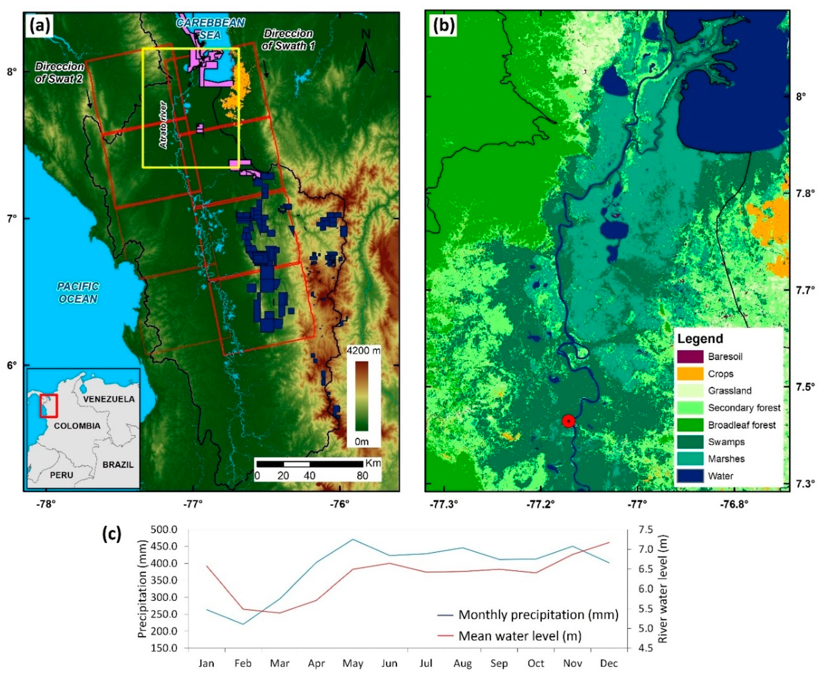
The Atrato River Basin is located in the biogeographical region of Chocó, Colombia (Figure 1), with headstream on the Western Andes mountain range and outlet into the Caribbean Sea. The basin occupies an area of 35,700 km2 and has an average annual precipitation of 5000 mm/year that reaches up to 12,000 mm/year in the upper basin [44]. It is considered to be one of the rainiest areas of the world [45,46]. The Atrato River basin presents a bimodal seasonal precipitation pattern with peak precipitation and runoff during May and November and a dry period that goes from January to April (Figure 1c). The basin is mostly flat, with an average slope of 0.04% and is mainly covered by forest and wetland marshes (88%), followed by disturbed lands (10%) used for agriculture, pastures, urban settlement, especially in its northeastern part, and water bodies (2%). Some fractions of the basin have been opened for mining, with large impacts on the main river channel (Figure 1a and Figure S1, Supplementary Materials). The front of colonization is extending rapidly from the east towards the Atrato floodplains, placing a threat to the natural dynamics of the ecosystems of the wetlands of the floodplain [34,35,37].
2.2. Data and Pre-processing
We here used DInSAR to obtain changes of water level in space and time that could shed some light regarding the state of hydrologic connectivity within the flood plain and that between the floodplain and the main channel upstream. In the general DInSAR approach [47], the interferometric phase includes the influence of the displacement, topography, atmosphere, and baseline (i.e., orbit location). The influence components of topography and baseline can be simulated and removed during the interferometric process using a digital elevation model and the orbit information [48]. In the atmosphere, the radiation ionizes neutral atoms forming a layer of free electrons around the earth, causing a delay in the SAR signal and in some cases affecting significantly the interferometric phase (especially in the case of L-band) [49,50,51]. It is important to mention that ionization highly depends on the sun’s activity and shows temporal and latitudinal variations [52]. Several techniques can be applied to estimate and correct the ionospheric phase delay such as the techniques using the Faraday rotation [53], estimating azimuth offsets [54], or using the range split-spectrum technique [50,55].
The ALOS-PALSAR 1 system was launched on June 2006 and operated until May 2011. This sensor operates at L-band (Center frequency 1.270 GHz) with a wavelength of 23.62 cm, with different polarizations (HH, HV, VV, VH), and a revisiting time of 46 days. In the present study, we used Single Look Complex (SLC) data in strip map mode, with single polarization HH available for the study area between 2008 and 2010. The SLC images retain both the amplitude and phase of the radar signal. The interferometric process requires at least two images of the same area collected at different times (repeat-pass observation), or at the same time but with different orbit, with one referred to as the master image, and the other is the slave image. These images are known as the interferometric pair.
We obtained ALOS data from the Alaska Satellite Facility online portal (https://vertex.daac.asf.alaska.edu/). Seven images were used for each scene of the first swath, and 8 images for each scene of the second swath. Both swaths were needed since the Atrato River and its floodplain are located precisely between these swaths. In total, we processed 60 acquisitions for the entire study area; all were acquired between May and September of each year (2008–2010). Since the interferometric image pairs were selected with a time lapse of less than 365, eight interferograms were obtained for each scene. Table 1 displays a summary of the interferograms, indicating the time lapse and the base line for each interferometric pair. All the scenes in both swaths were geo-coded to a spatial resolution of 25 m; have incident angles ranging between 36° and 41° and a HH polarization.
For the present study we used a repeat-pass observation, and we referred to the oldest image of the interferometric pair as the master image, and water level in the main channel of the Atrato River upstream during this acquisition as WL1, and to the most recent image as the slave image, and water level in the main channel of the Atrato River upstream during this acquisition as WL2. As such, we analyze and refer to the chronological changes in water level and resulting interferometric phase in chronological order.
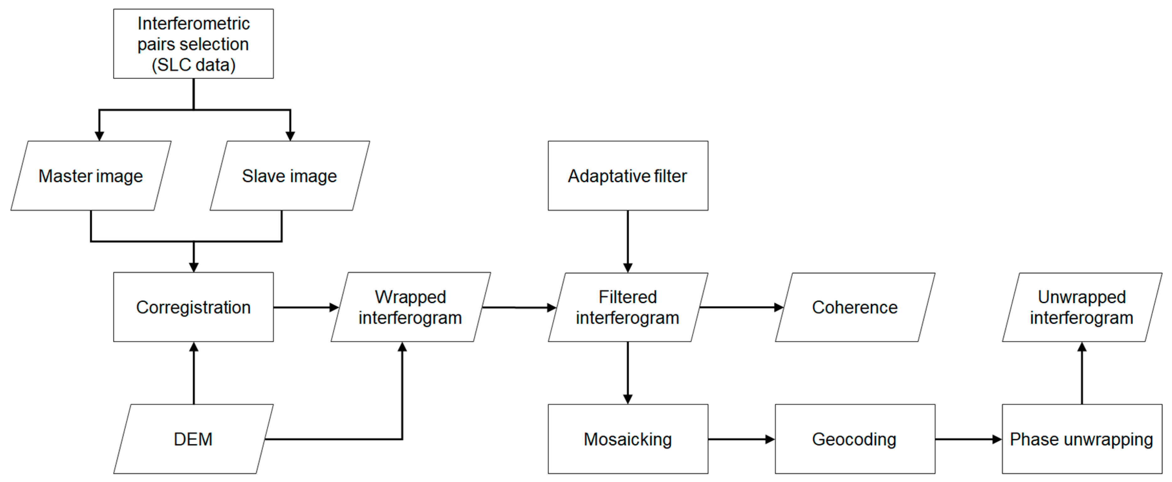
All interferometric pairs were processed using SARscape/ENVI version 5.5 (Harris Geospatial Solutions, Inc., Broomfield, CO, USA). The SLC master and slave data were co-registered with the 30 m Shuttle Radar Topography Mission (SRTM) digital elevation model (http://srtm.csi.cgiar.org/srtmdata/). This co-registration ensured that each object on the ground coincided with the same pixel in both images, i.e., master and slave. After co-registration, the interferograms (i.e., DInSAR phase maps between master and slave image) were generated by multiplying the master Single Look Complex data by the complex conjugate of the slave. Figure 2 shows the steps required to obtain the interferograms.
The 30 m SRTM digital elevation model was used to simulate the interferogram expected from topography, and remove it from the observed interferogram. The geodynamic processes could also affect the DInSAR phase, especially in regions with high rate of vertical displacements due to surface deformation and subsidence. In the present study, we compared the magnitude of the differences in water level between acquisitions obtained from the interferogram analysis, with surface displacement data, in order to determine the possible contribution of the latter to the fringe patterns observed. The displacement data was acquired from the GNSS station APTO from the SIRGAS-CON network available for the study area (http://www.sirgas.org/es/sirgas-con-network/stations/station-list/#).
The impact of ionosphere on the signal was not significant, most likely dues to the night imaging (local time 23:00). To verify this, we compared two example interferograms with and without ionospheric correction, using the range-split spectrum method [55] available in the ISCE software developed by the California Institute of Technology and Stanford University (UNAVCO, Boulder, Colorado, United States of America) [56] and found no distinct spatial patterns (see Figure S2 in Supplementary Materials). It is important to mention that ionospheric phase generally shows a smooth latitudinal variation across several kilometers with patterns unrelated to local geophysical features such as rivers and land cover [57].
To remove other effects related to temporal and geometric effect, we applied a Goldstein 5 × 5 phase filter to the interferogram [58]. This filter is commonly used and has been proved as an effective InSAR interferogram filter [59]. The observed interferometric fringe pattern (i.e., spatial gradient in DInSAR phase) is used to estimate the relative water level change in the wetland between the two radar acquisitions. The vertical water level change (Δh) can be obtained from the phase change between the two acquisitions as follows [60]:
where is the wavelength (23.62 cm), is the DInSAR phase and is the incident angle (for the images used, the incident angles range between 36° and 41°).
Interferometric coherence (γ) is a measurement of similarity between the two images of the interferometric pair and varies from 0 to 1, and hence describes the quality of the signal. It is defined as follows [61]:
where and are the signals in the first and second image, and * denotes the complex conjugate of S.
The greater the coherence, the more accurate is the estimation of the water level change. The coherence was calculated based on the filtered interferogram. Mosaics were generated with the interferograms corresponding to the scenes of each swath (Figure 1a) and the data was geo-coded to a spatial resolution of 25 m.
The DInSAR phase initially obtained by the software is “wrapped”, ranging in a 2π-cycle. We performed the unwrapping of the phase to obtain an absolute phase change by multiplying the interferogram with the correct number of π-cycles maintaining spatial consistency. The method used in the unwrapping process was the Minimum Cost Flow algorithm, available in the SARscape/ENVI version 5.5 (Harris Geospatial Solutions, Inc., Broomfield, CO, USA). The method is based on the algorithm proposed in [62]. The unwrapped phase changes could then finally be used to calculate water level changes between the two acquisitions in all coherent areas of the interferogram.
2.3. Surface Water Flow Analysis in the Atrato River Floodplains
The resulting interferograms represent the DInSAR phase of the signal received by the sensor, between the interferometric pair images and in each 25-m pixel. When the water levels in the floodplains increases or decreases, the interferogram has a non-zero phase. Our analysis focused on two main tasks: (1) to identify source and direction of flow through the floodplain through interpretation of the spatial and temporal fluctuations of the fringe patterns in each interferogram, and (2) to determine the relationship between the observed interferogram phase in the floodplain and the water level changes upstream in the main channel of the Atrato River.
For the tasks, we selected two regions of analysis taking into consideration topographic factors such as land cover and the occurrence of fringe patterns. While the first site is located downstream, in a flat topographic zone covered by flooded marshlands (i.e., herbaceous wetlands), the second is located in the mid-basin, where topography is irregular and land cover is predominantly swamps (i.e., wetlands with trees) (Figure 3 top and bottom, respectively).
In order to analyze the temporal fluctuations of the fringe patterns in the interferograms, we used two horizontal transects. The first transect is 8-km long and traced perpendicular to the axis of the main river (CT1; Figure 3), while the second is 40-km long, following the course of the main river, consisting of three straight sections (CT2; Figure 3). The water level (WL) in the main channel of the Atrato River upstream was obtained from the water level station in operation by the Colombian Institute of Hydrology, Meteorology and Environmental Studies IDEAM in the area (Figure 1b). We analyzed the DInSAR phase along each transect under three conditions of water level change in the main channel of the Atrato River: i) Water level increase (WL1 < WL2); no change (i.e., WL1 ≈ WL2); and water level decrease (WL1 > WL2).
Finally, we calculated the relationship between the DInSAR phase and the water level changes measured in the water level station. For this purpose, we traced five additional transects along different locations of the floodplains (T1 to T5 in Figure 3). We selected their locations taking into consideration the different land cover types, regions with a coherence value above 0.3, and the persistence of fringe patterns in the different interferograms. Finally, we estimated the relationship between the DInSAR phase along the transect and WL changes.
3. Results and Discussion
3.1. Spatial Distribution of DInSAR Phase Patterns
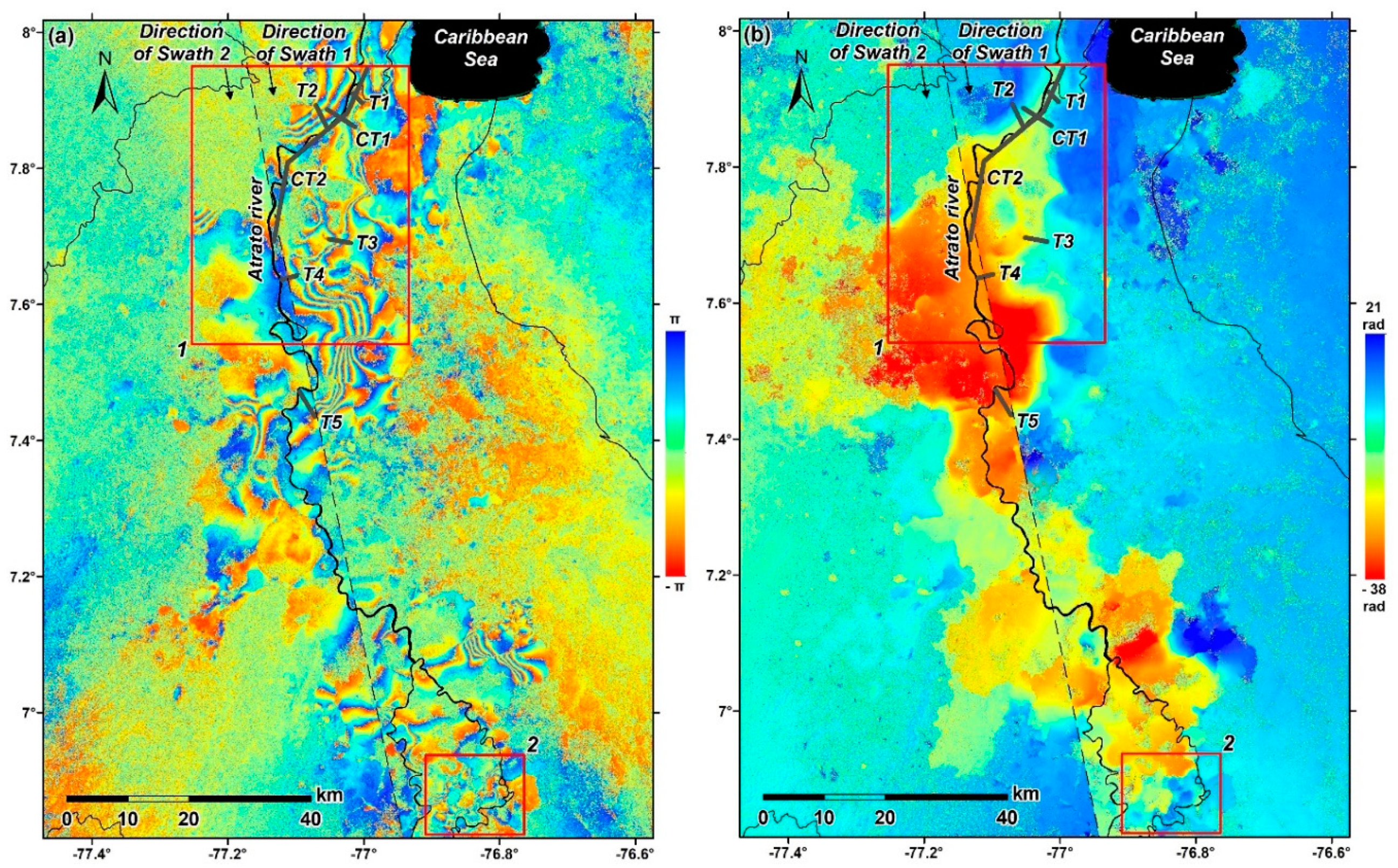
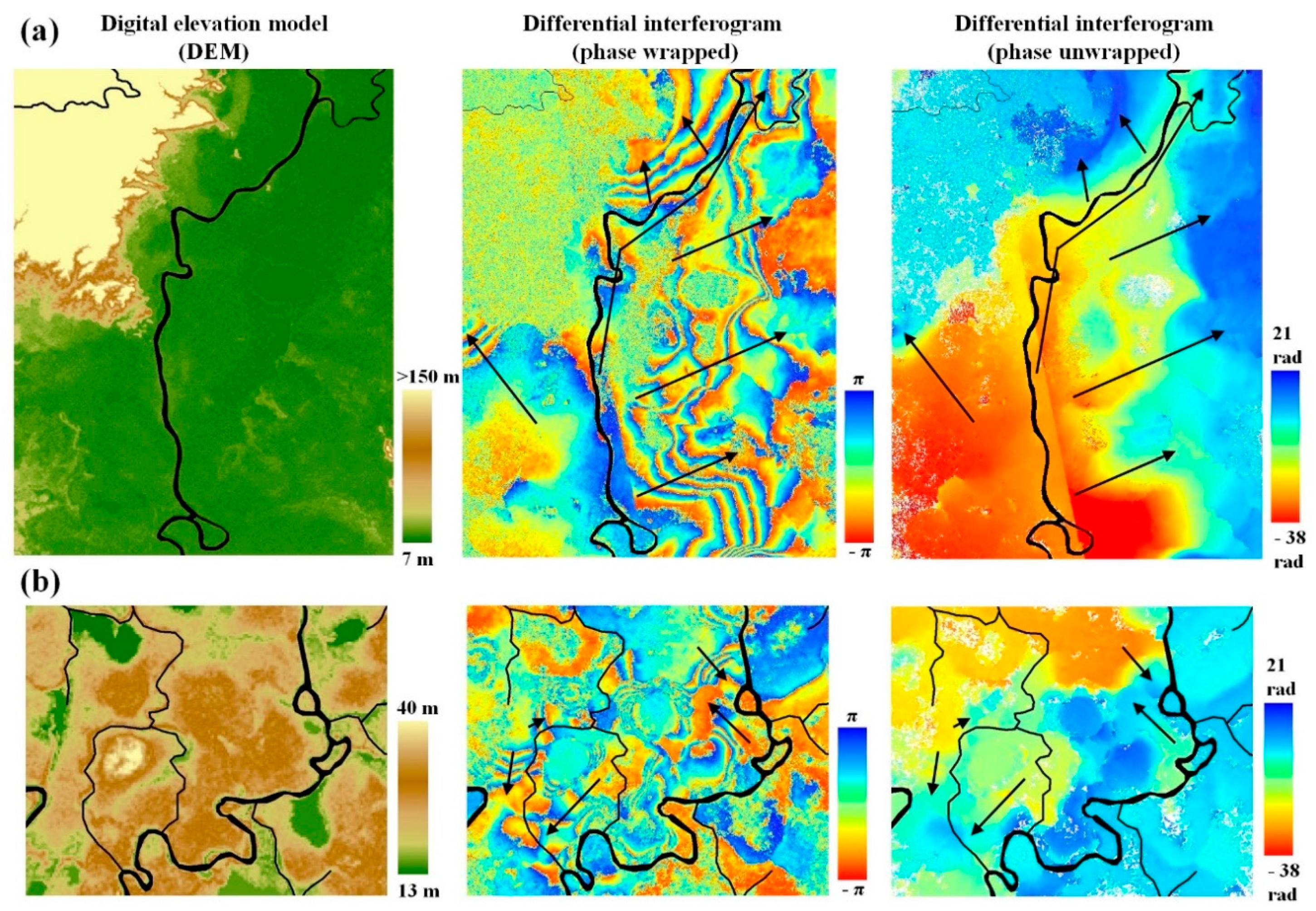
The interferogram with the highest coherence values, the shortest baseline and the greatest difference in water level is shown in Figure 3. This interferogram results from the pair of acquisitions taken in June 6 and September 6, 2010 in image swath one and June 23 to September 23 in image swath two. From Equation (1), each complete color cycle in the wrapped interferogram (Figure 3a) corresponds to a vertical change in water level of approximately 15.1 cm for an incidence angle of 38.7° (at the center of the scenes). This is a relative change in relation to a reference point assumed static. The geographical location of the fringe patterns (color ramps in Figure 3) adjacent to the Atrato River agree with those of recurrent flooding events and under flood hazard risk [43]. These areas are covered by both marshes and swamps. The red region in Figure 3b (latitude 7.5°, longitude −77.1°) shows the most pronounced phase change and water level change pattern occurring between the two acquisitions, indicating approximately 85 cm changes in water level (−38 radians in Figure 3b) and is located between a topographic depression in the terrain and the confluence of an important tributary of the Atrato River, the Riosucio River.
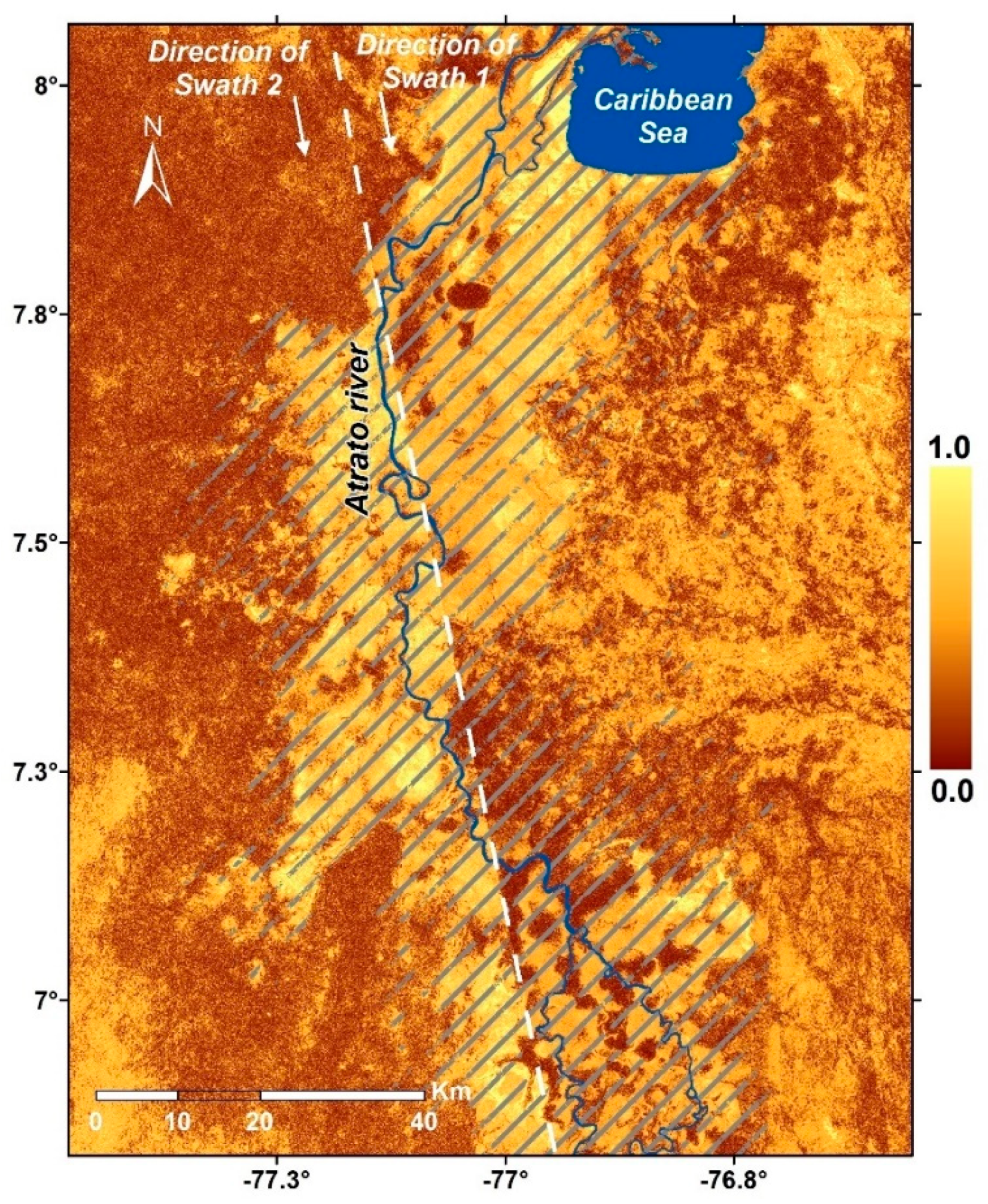
A coherence map is calculated by Equation (2) and presented in Figure 4. This map corresponds to the interferometric pairs of Figure 3. For the study area, the highest observed coherence regions (>0.5) are associated with swamps and marshes and the lowest to forests and agricultural areas and pastures.
A zoom to the downstream and middle sections of the Atrato River (Rectangles one and two in Figure 3, respectively) shows marked differences of surface water flow (Figure 5). Further downstream (Figure 5a), we found continuous and wide flow patterns with a predominantly parallel orientation to the axis of the main channel of the river. The magnitude of the DInSAR phase between acquisitions increases from the axis of the main channel of the river towards the floodplains. In the midsection of the basin (Figure 5b), the patterns are less continuous, patchy, and describe surface water flow in various directions, probably due to the irregular topography and high complexity of the wetland network. Water storage and direction of flows can be identified from these observations, providing crucial information to model flow processes, nutrient transport and biogeochemical cycles in the Atrato River. Similar discontinuous patterns have been found in previous studies on surface water flows in the floodplains of the Amazon, Congo, and Brahmaputra rivers, using JERS-1 data [19,63].
3.2. Temporal Fluctuations in the DInSAR Phase Patterns
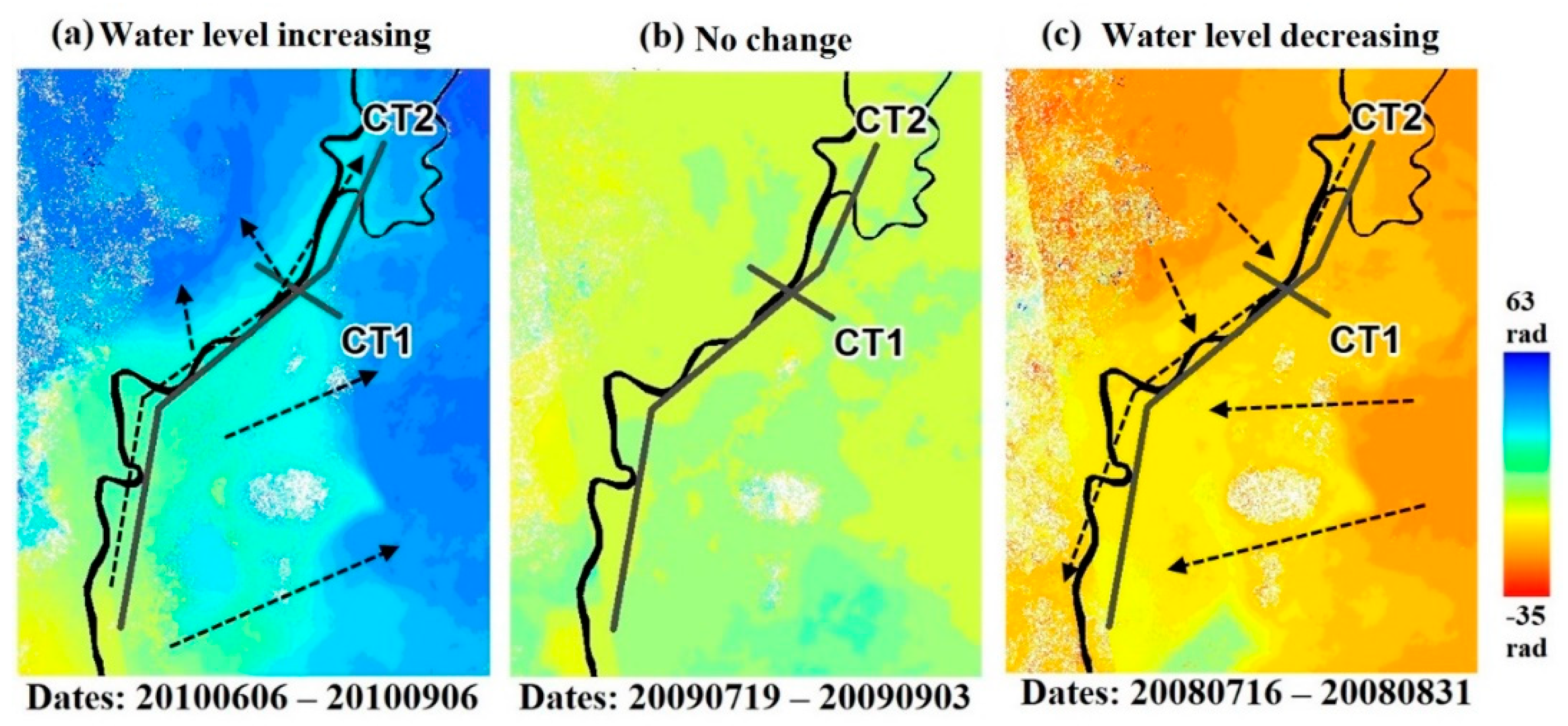
In order to study DInSAR phase patterns under different hydrologic scenarios (i.e., 1. water level increase, 2. no change in water level, and 3. water level decrease), we selected three interferograms representative of each of these three conditions (Figure 6). The first unwrapped interferogram represents water level changes in the floodplain that correspond to a water level increase in the station upstream of 1.1 m and the third to a decrease of −0.87 m. Dashed arrows in Figure 6 show the direction of increasing DInSAR phase. Positive DInSAR phase was found in the downstream direction in interferogram Figure 6a along the transect CT2 (from light green color and 18 radians to dark blue and 50 radians). Along CT1 direction, positive DInSAR phase was found as it moves away from the river axis. Conversely, in Figure 6c we found a negative DInSAR phase in the downstream direction along the transect CT2 (i.e., from yellow and −2 rad to orange color and −15 rad). Along CT1 direction, negative DInSAR phase was found as it moves away from the river axis. In the no change condition, Figure 6b, the DInSAR phase was negligible. Figure 6 represents how the floodplain “fills-up” and “empties” with water flow from and to the river.
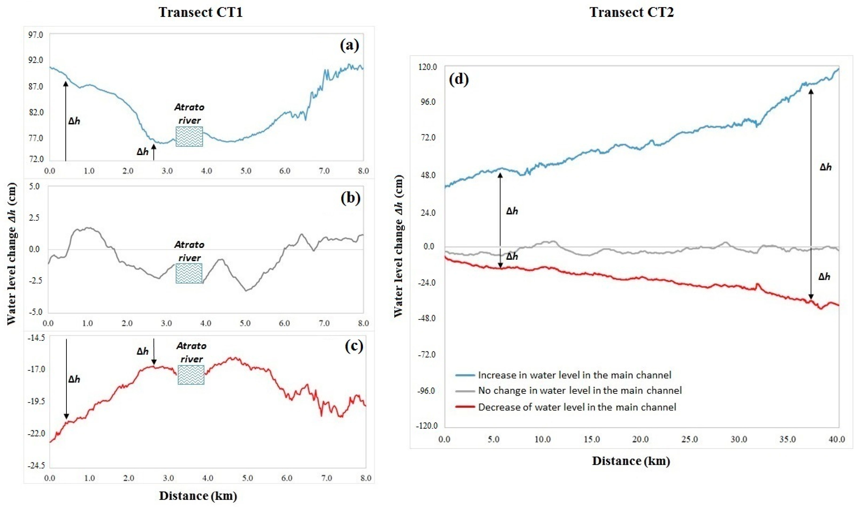
The Figure 7 shows the variation profiles of the water level change along transects CT1 and CT2. Water level change was calculated from DInSAR phase using equation 1. For C1, a convex behavior of the variation of the water level along the transect can be seen when the change in water level in the river is positive (Figure 7a), small wave-like variations of the water level along the transect when there is no change in water level in the river (Figure 7b), and a concave behavior of the variation of the water level along the transect when the change in water level in the river is negative (Figure 7c). As such, an increase in water level in the main channel had positive and larger Δh along the transects, whereas large but negative Δh was found with a decrease in water level in the main channel. In general terms, the magnitude of the Δh always increases when moving away from the main river channel. Figure 7d shows the variation in Δh for the CT2 transect, which has a longitude of 40.0 km. In a similar way, we also found increasing absolute Δh in the direction of the flow of the river downstream for increasing water level in the main channel. A similar pattern was found in the Amazon River [13] and Ciénaga Grande de Santa Marta, Colombia [8], whereas an observed increase in the discharge of the river corresponded with increasing Δh and water level in the downstream direction.
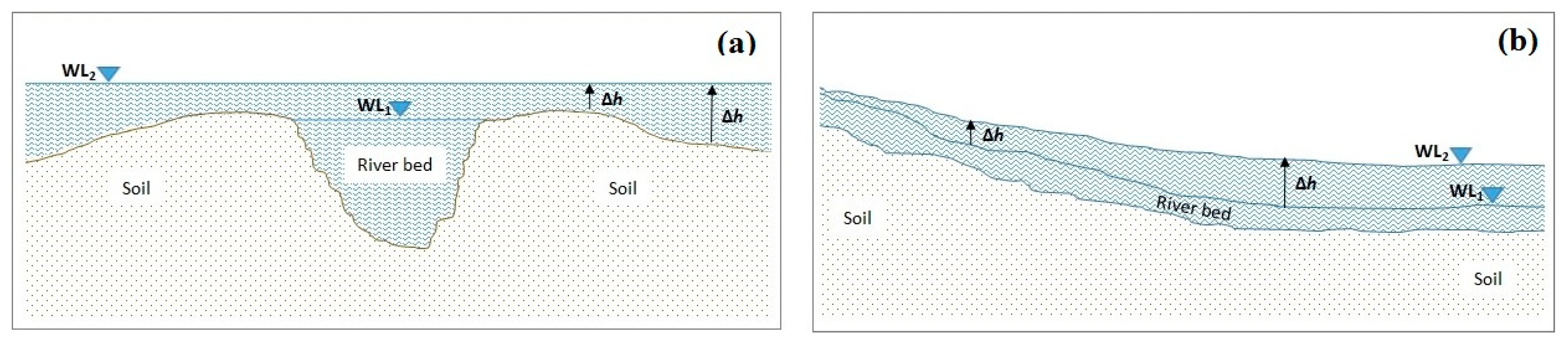
From the previous analysis, we derived the direction of surface water flow in the floodplains from the retrieved water level changes and river conditions across the transects CT1 and CT2. In CT1, an increase in water level in the main channel (Figure 7a) denotes a change from a water level profile WL1 to WL2 (Figure 8a). Under this condition, the water flows from the axis of the river outwards and it appears on the interferogram as a positive change of phase. On the other hand, a negative change in the water level (Figure 7c) denotes a change from WL2 to WL1 in Figure 8a, with corresponding negative water level change. The derived water level profiles along transect C2 for increasing and decreasing water levels in the main channel evidence a decreasing river channel slope and transition to floodplain with an already flooded plain in the first time period.
3.3. Relationship between Water Changes in the Main Channel Upstream and Floodplain
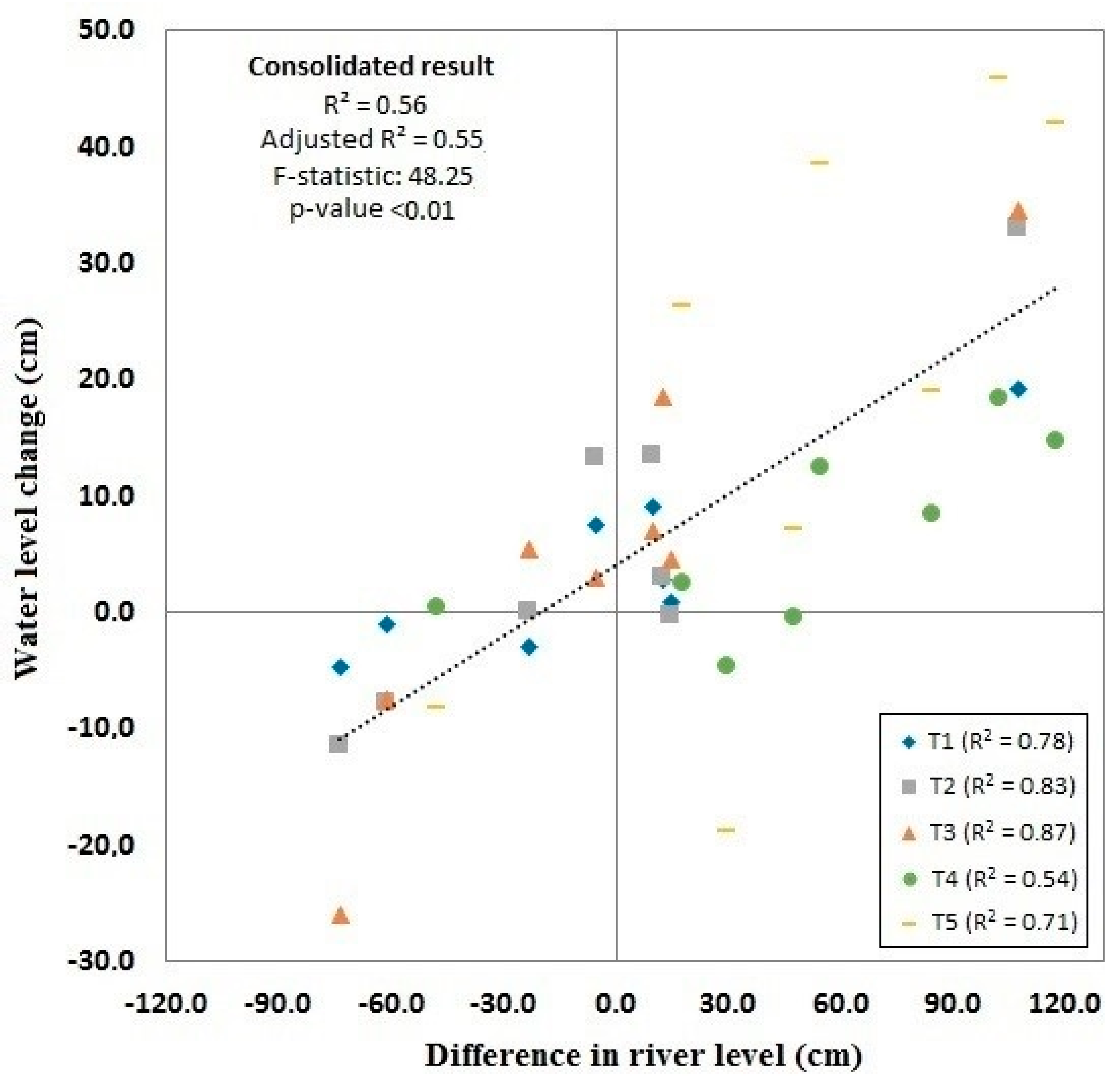
Figure 9 shows the linear relationships and coefficients of determination between the water level change Δh along the transects T1 to T5 obtained from DInSAR and the water level change in the measuring station on the main channel upstream, for the dates of the images in each interferogram. First of all, most changes in water level change calculated by DInSAR along the transects are considerably larger than the vertical surface displacement registered in the Global Navigation Satellite System (GNSS) station located in the study area (See Figure S3, Supplementary Materials). The station gives evidence to a negative vertical displacement rate occurring in the region of about 0.72 cm/year. As such, the maximum vertical surface displacement in the interferograms occurs in the interferogram with temporal baseline of 322 days (Table 1); and corresponding to approximately 0.63 cm of surface change. Most of the water level changes shown in the interferograms and across the transects are far larger than the 0.63 cm threshold, evidencing that the surface water level changes observed along the transects of our study are mainly due to hydrological processes and not due to the regions surface displacement as observed in the GNSS station.
The transects located in areas with swamps (T4 and T5) show relative smaller linear relationships with R2 values (around 0.5) in comparison to the transects located in areas with marshes (T1, T2 and T3), where R2 values reach 0.87. This is evidence of different hydrological processes occurring in the two ecosystems and determining the characteristics of surface water flow. Furthermore, the forests may not be as dependent on the sheet flow coming from the main channel as the marshes to due to topographical features or contributing tributaries in the vicinity that may lower the influence of local water flow on the changes along the main river channel.
When all the transects are analyzed together, we found a significant positive relation between water level change in the main river and the water level changes calculated from DInSAR phase in all transects T1 to T5 in the floodplain (R2 = 0.56; Adjusted R2 = 0.55; F-statistic: 48.25; p = 2.9 × 10⁻⁸ < 0.01). Hence, the changes in the water level upstream could explain more than 56% of the DInSAR phase along the transects of the floodplain and corresponding changes in water level. This is surprising since the transects are spread out across different locations in the floodplain, with no consistent alignment in relation to the direction of flow of the main channel (see Figure 5). The relatively high coefficients of determination indicate good hydrological connectivity between the river and its floodplain. These observations contrast with previous studies in the Ciénaga Grande of Santa Marta, Colombia [8] where the tidal influence, the development of infrastructure, and the artificial regulation of the flow of water towards the Ciénaga have affected dramatically the hydrological connectivity within the deltaic wetland system and the main river channel upstream. In this study, water discharge upstream on the main tributary of the wetland could explain at most 17% of the variance of the change in water level in the wetland as calculated by DInSAR.
4. Conclusions
The interferograms resulting from this study provide an important tool for understanding the complex dynamics of surface water flow in the floodplains of the Atrato River. We found that the spatial and temporal changes in the surface water flow of the floodplains is conditioned mainly by the fluctuations in the main channel of the river, while in the middle part of the basin, topography and the complex network of channels and tributaries also have an important influence. The DInSAR phase is positively related to the changes in the water level of the main channel of the Atrato River, and we assume that this signals natural and good hydrologic connectivity between river and floodplain. As such, it appears that mining and agricultural activities in the floodplain, as of 2010, have not significantly affected the hydrological connectivity in the lower basin. The information resulting from this study can be used as input for the calibration and validation of hydrological models in ungauged floodplains such as the Atrato River floodplain. Furthermore, this study describes, for the first time, the spatiotemporal surface water flow patterns of the region using InSAR techniques in the study area. This study demonstrates the potential of DInSAR for continuous monitoring of hydrological processes in the Atrato River, Colombia. The analysis and results presented here, also provides a foundation to improve our understanding of the complex hydrological dynamics of the Atrato river floodplain. Finally, we recommend our analysis of flow connectivity serve as a baseline against which to assess the consequences of agricultural and mining expansion on regional hydrology.
Supplementary Materials
The following are available online at https://www.mdpi.com/2073-4441/11/5/875/s1, Figure S1: Ecosystem degradation by mining activities in the Quito River, a tributary of the Atrato River, Figure S2: Ionospheric correction analysis for the study area, Figure S3: Time series of the APTO SIRGAS-CON network station.
Author Contributions
Conceptualization, S.P.-Á. and F.J.; Methodology, S.P.-Á. and F.J.; Software, S.P.-Á. and F.J.; Validation, S.P.-Á., T.-H.L.; Formal analysis, S.P.-Á., J.A.A.-A. and F.J.; Investigation, S.P.-Á. and F.J.; resources, S.P.-Á., J.A.A.-A., M.S. and F.J.; data curation, S.P.-Á. and F.J.; writing—original draft preparation, S.P.-Á.; writing—review and editing, S.P.-Á., J.A.-A., M.S., T.-H.L. and F.J.; visualization, S.P.-Á. and F.J.; supervision, J.A.A.-A., F.J. and M.S.; project administration, F.J. and M.S.; funding acquisition, F.J. and M.S.
Funding
This research was funded by the Colombian Department of Science, Technology and Innovation (COLCIENCIAS), under the High-level training program National Doctorates scholarship (Call code 647 for 2014). The Swedish Research Council (VR, project 2015-06503) and the Swedish Research Council for Environment, Agricultural Sciences and Spatial Planning FORMAS (942-2015-740) have also funded this study. The Swedish Foundation for International Cooperation in Research and Higher Education (STINT) project IB2018-7494 has also funded traveling and publishing of this study.
Acknowledgments
Part of this work was performed at the Jet Propulsion Laboratory, California Institute of Technology. PALSAR data was obtained from the Vertex data portal of the Alaska Satellite Facility. The onsite measuring station data was obtained from the Colombian Institute of Hydrology, Meteorology and Environmental Studies in Colombia (IDEM) online portal.
Conflicts of Interest
The authors declare no conflict of interest.
References
- Hamilton, S.K.; Sippel, S.J.; Melack, J.M. Comparison of inundation patterns among major South American floodplains. J. Geophys. Res. Atmos. 2002, 107, 8038. [Google Scholar] [CrossRef]
- Melack, J.M. Interactions between Biosphere, Atmosphere and Human Land Use in the Amazon Basin; Nagy, L., Forsberg, B., Artaxo, P., Eds.; Springer: Berlin, Germany, 2016; pp. 117–145. [Google Scholar]
- Thorslund, J.; Jarsjo, J.; Jaramillo, F.; Jawitz, J.W.; Manzoni, S.; Basu, N.B.; Chalov, S.R.; Cohen, M.J.; Creed, I.F.; Goldenberg, R.; et al. Wetlands as large-scale nature-based solutions: Status and challenges for research, engineering and management. Ecol. Eng. 2017, 108, 489–497. [Google Scholar] [CrossRef]
- Audesirk, T.; Audesirk, G.; Bruce, E. Biología: La vida en la Tierra; Prentice Hall Inc.: Upper Saddle River, NJ, USA, 2008. [Google Scholar]
- Melack, J.M.; Engle, D. An organic carbon budget for an Amazon floodplain lake. Int. Ver. Theor. Angew. Limnol. Verh. 2009, 30, 1179–1182. [Google Scholar] [CrossRef]
- Richey, J.E.; Melack, J.M.; Aufdenkampe, A.K.; Ballester, V.M.; Hess, L.L. Outgassing from Amazonian rivers and wetlands as a large tropical source of atmospheric CO2. Nature 2002, 416, 617. [Google Scholar] [CrossRef] [PubMed]
- Pontes, P.R.M.; Fan, F.M.; Fleischmann, A.S.; de Paiva, R.C.D.; Buarque, D.C.; Siqueira, V.A.; Jardim, P.F.; Sorribas, M.V.; Collischonn, W. MGB-IPH model for hydrological and hydraulic simulation of large floodplain river systems coupled with open source GIS. Environ. Model. Softw. 2017, 94, 1–20. [Google Scholar] [CrossRef]
- Jaramillo, F.; Brown, I.; Castellazzi, P.; Espinosa, L.; Guittard, A.; Hong, S.-H.; Rivera-Monroy, V.H.; Wdowinski, S. Assessment of hydrologic connectivity in an ungauged wetland with InSAR observations. Environ. Res. Lett. 2018, 13, 24003. [Google Scholar] [CrossRef] [Green Version]
- Wemple, B.C.; Browning, T.; Ziegler, A.D.; Celi, J.; Chun, K.P.; Jaramillo, F.; Leite, N.K.; Ramchunder, S.J.; Negishi, J.N.; Palomeque, X.; et al. Ecohydrological disturbances associated with roads: Current knowledge, research needs, and management concerns with reference to the tropics. Ecohydrology 2018, 11, e1881. [Google Scholar]
- Van Meter, K.J.; Basu, N.B. Signatures of human impact: Size distributions and spatial organization of wetlands in the Prairie Pothole landscape. Ecol. Appl. 2015, 25, 451–465. [Google Scholar] [CrossRef]
- Quin, A.; Jaramillo, F.; Destouni, G. Dissecting the ecosystem service of large-scale pollutant retention: The role of wetlands and other landscape features. Ambio 2015, 44, 127–137. [Google Scholar] [CrossRef] [Green Version]
- Alsdorf, D.E.; Lettenmaier, D.P. Tracking Fresh Water from Space. Science 2003, 301, 1491–1494. [Google Scholar] [CrossRef]
- Cao, N.; Lee, H.; Jung, C.H.; Yu, H. Estimation of Water Level Changes of Large-Scale Amazon Wetlands Using ALOS2 ScanSAR Differential Interferometry. Remote Sens. 2018, 10, 966. [Google Scholar] [CrossRef]
- Schulz, J.; Albert, P.; Behr, H.-D.; Caprion, D.; Deneke, H.; Dewitte, S.; Dürr, B.; Fuchs, P.; Gratzki, A.; Hechler, P.; et al. Operational climate monitoring from space: The EUMETSAT satellite application facility on climate monitoring (CM-SAF). Atmos. Chem. Phys. 2008, 8, 8517–8563. [Google Scholar] [CrossRef]
- Wdowinski, S.; Hong, S. Wetland InSAR: A review of the technique and applications. In Remote Sensing of Wetlands; CRC Press: Boca Raton, FL, USA, 2015; pp. 154–171. [Google Scholar]
- Xie, C.; Shao, Y.; Xu, J.; Wan, Z.; Fanga, L. Analysis of ALOS PALSAR InSAR data for mapping water level changes in International Journal of Remote Analysis of ALOS PALSAR InSAR data for mapping water level changes in Yellow River Delta wetlands. Int. J. Remote Sens. 2013, 34, 2047–2056. [Google Scholar] [CrossRef]
- Alsdorf, D.E.; Smith, L.C.; Melack, J.M. Amazon floodplain water level changes measured with interferometric SIR-C radar. IEEE Trans. Geosci. Remote Sens. 2001, 39, 423–431. [Google Scholar] [CrossRef]
- Poncos, V.; Teleaga, D.; Bondar, C.; Oaie, G. A new insight on the water level dynamics of the Danube Delta using a high spatial density of SAR measurements. J. Hydrol. 2013, 482, 79–91. [Google Scholar] [CrossRef]
- Jung, H.C.; Hamski, J.; Durand, M.; Alsdorf, D.; Hossain, F.; Lee, H.; Hossain, K.; Hasan, A.K.M.A.; Khan, A.S.; Hoque, A.K.M.Z. Characterization of complex fluvial systems using remote sensing of spatial and temporal water level variations in the Amazon, Congo, and Brahmaputra Rivers. Earth Surf. Process. Landf. 2010, 35, 294–304. [Google Scholar] [CrossRef]
- Yuan, T.; Lee, H.; Jung, H.C. Congo Floodplain Hydraulics using PALSAR InSAR and Envisat Altimetry Data. In Remote Sensing of Hydrological Extremes; Lakshmi, V., Ed.; Springer: Cham, Switzerland, 2017. [Google Scholar]
- Oliver-Cabrera, T.; Wdowinski, S. InSAR-Based Mapping of Tidal Inundation Extent and Amplitude in Louisiana Coastal Wetlands. Remote Sens. 2016, 8, 393. [Google Scholar] [CrossRef]
- Ferretti, A.; Prati, C.; Rocca, F. Permanent scatterers in SAR interferometry. IEEE Trans. Geosci. Remote Sens. 2001, 39, 8–20. [Google Scholar] [CrossRef] [Green Version]
- Arnesen, A.S.; Silva, T.; Hess, L.; Novo, E.; Rudorff, C.M.; Chapman, B.; McDonald, K.C. Monitoring flood extent in the lower Amazon River floodplain using ALOS/PALSAR ScanSAR images. Remote Sens. Environ. 2013, 130, 51–61. [Google Scholar] [CrossRef]
- Evans, T.; Costa, M.; Telmer, K.; Silva, T. Using ALOS/PALSAR and RADARSAT-2 to Map Land Cover and Seasonal Inundation in the Brazilian Pantanal. IEEE J. Sel. Top. Appl. Earth Obs. Remote Sens. 2010, 4, 560–575. [Google Scholar] [CrossRef]
- Hoekman, D.; Vissers, M.A.A.; Wielaard, N. PALSAR Wide-Area Mapping of Borneo: Methodology and Map Validation. IEEE J. Sel. Top. Appl. Earth Obs. Remote Sens. 2010, 3, 605–617. [Google Scholar] [CrossRef]
- Alsdorf, D.E.; Melack, J.M.; Dunne, T.; Mertes, L.A.K.; Hess, L.L.; Smith, L.C. Interferometric radar measurements of water level changes on the Amazon flood plain. Nature 2000, 404, 174. [Google Scholar] [CrossRef] [PubMed]
- Reiche, J.; Lucas, R.; Mitchell, A.L.; Verbesselt, J.; Hoekman, D.H.; Haarpaintner, J.; Kellndorfer, J.M.; Rosenqvist, A.; Lehmann, E.; Woodcock, C.E.; et al. Combining satellite data for better tropical forest monitoring. Nat. Clim. Chang. 2016, 6, 120–122. [Google Scholar] [CrossRef]
- Kovacs, J.M.; Lu, X.X.; Flores-Verdugo, F.; Zhang, C.; Flores de Santiago, F.; Jiao, X. Applications of ALOS PALSAR for monitoring biophysical parameters of a degraded black mangrove (Avicennia germinans) forest. ISPRS J. Photogramm. Remote Sens. 2013, 82, 102–111. [Google Scholar] [CrossRef]
- Gudmundsson, S.; Sigmundsson, F. Three-dimensional surface motion maps estimated from combined interferometric synthetic aperture radar and GPS data. J. Geophys. Res. 2002, 107, 1–14. [Google Scholar] [CrossRef]
- Farolfi, G.; Bianchini, S.; Casagli, N. Integration of GNSS and Satellite InSAR Data: Derivation of Fine-Scale Vertical Surface Motion Maps of Po Plain, Northern Apennines, and Southern Alps, Italy. IEEE Trans. Geosci. Remote Sens. 2019, 57, 319–328. [Google Scholar] [CrossRef]
- McGlynn, B.L.; Blöschl, G.; Borga, M.; Bormann, H.; Hurkmans, R.; Komma, J.; Nandagiri, L.; Uijlenhoet, R.; Wagener, T. A data acquisition framework for predictions of runoff in ungauged basins. In Run-Off Prediction in Ungauged Basins: Synthesis Across Processes, Places and Scales; Cambridge University Press: Cambridge, UK, 2013; pp. 29–51. [Google Scholar]
- Hidayat, H.; Teuling, A.J.; Vermeulen, B.; Taufik, M.; Kastner, K.; Geertsema, T.J.; Bol, D.C.C.; Hoekman, D.H.; Haryani, G.S.; Van Lanen, H.A.J.; et al. Hydrology of inland tropical lowlands: The Kapuas and Mahakam wetlands. Hydrol. Earth Syst. Sci. 2017, 21, 2579–2594. [Google Scholar] [CrossRef]
- Myers, N.; Mittermeier, R.A.; Mittermeier, C.G.; da Fonseca, G.A.B.; Kent, J. Biodiversity hotspots for conservation priorities. Nature 2000, 403, 853–858. [Google Scholar] [CrossRef] [PubMed]
- Anaya-Acevedo, J.A.; Escobar-Martínez, J.F.; Massone, H.; Booman, G.; Quiroz-Londoño, O.M.; Cañón-Barriga, C.C.; Montoya-Jaramillo, L.J.; Palomino-Ángel, S. Identification of wetland areas in the context of agricultural development using remote sensing and GIS. DYNA 2017, 84, 201. [Google Scholar]
- Patino, J.E.; Estupinan-Suarez, L. Hotspots of Wetland Area Loss in Colombia. Wetlands 2016, 36, 935–943. [Google Scholar] [CrossRef]
- Survey of Territories Affected by Illicit Crops-2016. Available online: https://www.unodc.org/documents/crop-monitoring/Colombia/Colombia_Coca_survey_2016_English_web.pdf (accessed on 9 April 2019).
- Gómez, L.F.; Suárez, C.F.; Trujillo, A.F.; Bravo, A.M.; Rojas, V.; Hernandez, N.; Vargas, M.C. Landscape Management in Chocó-Darién Priority Watersheds; WWF-Colombia: Bogotá, Colombia, 2014. [Google Scholar]
- Hurtado, A.; Santamaría, M.; Matallana-Tobón, C.L. Plan de Investigación y Monitoreo del Sistema Nacional de Áreas Protegidas (Sinap): Avances Construidos desde la Mesa de Investigación y Monitoreo Entre 2009 y 2012; Instituto de Investigación de Recursos Biológicos Alexander von Humboldt: Bogotá, Colombia, 2013. [Google Scholar]
- Klemas, V. Remote sensing of emergent and submerged wetlands: An overview. Int. J. Remote Sens. 2013, 34, 6286–6320. [Google Scholar] [CrossRef]
- King, B.; Yurco, K.; Young, K.R.; Crews, K.A.; Shinn, J.E.; Eisenhart, A.C. Livelihood Dynamics Across a Variable Flooding Regime. Hum. Ecol. 2018, 46, 865–874. [Google Scholar] [CrossRef]
- Estupinan-Suarez, L.M.; Florez-Ayala, C.; Quinones, M.J.; Pacheco, A.M.; Santos, A.C. Detection and characterization of Colombian wetlands: Integrating geospatial data with remote sensing derived data. Using ALOS PALSAR and MODIS imagery. Int. Arch. Photogramm. Remote Sens. Spat. Inf. Sci. ISPRS Arch. 2015, 40, 375–382. [Google Scholar] [CrossRef]
- Mosquera-Machado, S.; Ahmad, S. No TitleFlood hazard assessment of Atrato River in Colombia. Water Resour. Manag. 2007, 21, 591–609. [Google Scholar] [CrossRef]
- Martinez-Ortega, E.F.; Mena, D.; Bernal, F. Modelación Hidrológica de la Cuenca alta del rio Atrato Mediante HEC-HMS, para la Determinación de Caudales Máximos; IDEAM: Bogotá, Colombia, 2014.
- Palomino-Ángel, S.; Anaya-Acevedo, J.A.; Botero, B.A. Evaluation of 3B42V7 and IMERG daily-precipitation products for a very high-precipitation region in northwestern South America. Atmos. Res. 2019, 217, 37–48. [Google Scholar] [CrossRef]
- Chen, M.; Xie, P.; Janowiak, J.E.; Arkin, P.A. Global Land Precipitation: A 50-yr Monthly Analysis Based on Gauge Observations. J. Hydrometeorol. 2002, 3, 249–266. [Google Scholar] [CrossRef]
- Adler, R.F.; Huffman, G.J.; Chang, A.; Ferraro, R.; Xie, P.; Janowiak, J.; Rudolf, B.; Schneider, U.; Curtis, S.; Bolvin, D.; et al. The Version-2 Global Precipitation Climatology Project (GPCP) Monthly Precipitation Analysis (1979–Present). J. Hydrometeorol. 2003, 4, 1147–1167. [Google Scholar] [CrossRef] [Green Version]
- Bamler, R.; Hartl, P. Synthetic aperture radar interferometry. Inverse Probl. 1998, 14, 55. [Google Scholar] [CrossRef]
- Massonnet, D.; Feigl, K.L. Radar interferometry and its application to changes in the Earth’s surface. Rev. Geophys. 1998, 36, 441–500. [Google Scholar] [CrossRef]
- Gray, A.L.; Mattar, K.E.; Sofko, G. Influence of Ionospheric Electron Density Fluctuations on Satellite Radar Interferometry streaking’ and the ionosphere. Geophys. Res. Lett. 2000, 27, 1451–1454. [Google Scholar] [CrossRef]
- Rosen, P.A.; Hensley, S.; Chen, C. Measurement and mitigation of the ionosphere in L-band Interferometric SAR data. In Proceedings of the 2010 IEEE Radar Conference, Washington, DC, USA, 10–14 May 2010; pp. 1459–1463. [Google Scholar]
- Meyer, F.; Bamler, R.; Jakowski, N.; Fritz, T. The Potential of Low-Frequency SAR Systems for Mapping Ionospheric TEC Distributions. IEEE Geosci. Remote Sens. Lett. 2006, 3, 560–564. [Google Scholar] [CrossRef]
- Zolesi, B.; Cander, L.R. Ionospheric Prediction and Forecasting; Springer: Berlin/Heidelberg, Germany, 2014. [Google Scholar]
- Rignot, E.J.M. Effect of Faraday rotation on L-band interferometric and polarimetric synthetic-aperture radar data. IEEE Trans. Geosci. Remote Sens. 2000, 38, 383–390. [Google Scholar] [CrossRef] [Green Version]
- Chen, A.C.; Zebker, H.A. Reducing Ionospheric Effects in InSAR Data Using Accurate Coregistration. IEEE Trans. Geosci. Remote Sens. 2014, 52, 60–70. [Google Scholar] [CrossRef]
- Fattahi, H.; Simons, M.; Agram, P. InSAR Time-Series Estimation of the Ionospheric Phase Delay: An Extension of the Split Range-Spectrum Technique. IEEE Trans. Geosci. Remote Sens. 2017, 55, 5984–5996. [Google Scholar] [CrossRef]
- Rosen, P.A.; Gurrola, E.; Sacco, G.F.; Zebker, H. The InSAR scientific computing environment. In Proceedings of the EUSAR 2012 9th European Conference on Synthetic Aperture Radar, Nürnberg, Germany, 23–26 April 2012; pp. 730–733. [Google Scholar]
- Shim, J.S. Analysis of Total Electron Content (TEC) Variations in the Low- and Middle-Latitude Ionosphere; Utah State University: Logan, UT, USA, 2009. [Google Scholar]
- Goldstein, R.M.; Werner, C.L. Radar interferogram filtering for geophysical applications. Geophys. Res. Lett. 1997, 25, 4035–4038. [Google Scholar] [CrossRef]
- Song, R.; Guo, H.; Liu, G.; Perski, Z.; Fan, J. Improved Goldstein SAR interferogram filter based on empirical mode decomposition. IEEE Geosci. Remote Sens. Lett. 2014, 11, 399–403. [Google Scholar] [CrossRef]
- Lu, Z.; Kwoun, O. Radarsat-1 and ERS InSAR Analysis Over Southeastern Coastal Louisiana: Implications for Mapping Water-Level Changes Beneath Swamp Forests. IEEE Trans. Geosci. Remote Sens. 2008, 46, 2167–2184. [Google Scholar] [CrossRef]
- Woodhouse, I.H. Introduction to Microwave Remote Sensing; Taylor & Francis Group: Boca Raton, FL, USA, 2006. [Google Scholar]
- Costantini, M. A novel phase unwrapping method based on network programming. IEEE Trans. Geosci. Remote Sens. 1998, 36, 813–821. [Google Scholar] [CrossRef]
- Alsdorf, D.; Bates, P.; Melack, J.; Wilson, M.; Dunne, T. Spatial and temporal complexity of the Amazon flood measured from space. Geophys. Res. Lett. 2007, 34. [Google Scholar] [CrossRef] [Green Version]
Figure 1.
(a) Location of the study area and Atrato River basin (black) with the digital elevation model presented in the background. The red squares refer to the scenes of PALSAR data used in this study and belonging to two different swaths. Agricultural areas in the northeastern part of the basin are presented in orange. Mining concessions in the basin are presented in blue and projected mining concessions are presented in purple. (b) Zoom of the yellow square of (a) showing land cover in the study area derived from a classification of a Landsat 8 data time series, and the only water level station on the main river upstream of the floodplain (red dot). (c) Average monthly precipitation (for the period 2000–2018) in the Atrato River Basin and average water level (for the period 2000–2018) at the station on the main river channel located upstream.

Figure 2.
The interferometric processing chain of PALSAR data in this study.

Figure 3.
Interferograms showing the (a) wrapped and (b) unwrapped DInSAR phase in the floodplains. The dates (year-month-day) of the master-slave images used to generate the interferogram are 20100606–20100906 on swath one and 20100623–20100923 on swath two. The dashed line represents the limit between the two swaths. Transects CT1 (8 km) and CT2 (40 km) were used to analyze the temporal fluctuation of the water level and transects T1, T2, T3, T4 and T5 were used to analyze the relation between water level change in the floodplains and water level change in the water level station on the main river channel upstream. The red rectangles 1 and 2 are zoomed in Figure 5.

Figure 4.
Coherence map. The dates (year-month-day) of the master-slave images used are 20100606–20100906 on swath one and 20100623–20100923 on swath two. The white dashed line represents the limit between the two swaths. The area demarcated by gray diagonal lines correspond to marshes and swamps.
Figure 4.
Coherence map. The dates (year-month-day) of the master-slave images used are 20100606–20100906 on swath one and 20100623–20100923 on swath two. The white dashed line represents the limit between the two swaths. The area demarcated by gray diagonal lines correspond to marshes and swamps.

Figure 5.
Zooms of Red squares (a) Nr. 1 and (b) 2 in Figure 3 with the digital elevation model, the wrapped and the unwrapped phase interferograms. The black lines correspond to the main channel of the Atrato River and its tributaries. The arrows indicate the direction of water flow resulting from the DInSAR phase.

Figure 6.
Unwrapped interferograms for (a) increasing water level change in the main channel of the Atrato River, (b) no water level change and (c) decreasing water level. The dashed arrows indicate the direction of increasing DInSAR phase and hence water level change.
Figure 6.
Unwrapped interferograms for (a) increasing water level change in the main channel of the Atrato River, (b) no water level change and (c) decreasing water level. The dashed arrows indicate the direction of increasing DInSAR phase and hence water level change.

Figure 7.
Water level change Δh under three conditions in the main river in transect CT1 perpendicular to the river axis with (a) water level increase in the main river; (b) no change in the water level in the main river; (c) water level decrease in the main river. (d) Water level change Δh in transect CT2 parallel to the river axis. The blue line corresponds the DInSAR phase along the transect for the water level increase condition, the gray line corresponds to the condition of no change, and the red line corresponds to the condition of water level decrease in the main channel.

Figure 8.
Description of the surface water flow in the floodplains. (a) Cross-sectional profiles of water level across the perpendicular transect CT1 and (b) the longitudinal profile parallel to the direction of flow of the main channel of the Atrato River CT2.
Figure 8.
Description of the surface water flow in the floodplains. (a) Cross-sectional profiles of water level across the perpendicular transect CT1 and (b) the longitudinal profile parallel to the direction of flow of the main channel of the Atrato River CT2.

Figure 9.
Linear relationships and coefficients of determination between the water level change Δh along the transects T1 to T5 and the water level change in the measuring station on the main channel upstream.
Figure 9.
Linear relationships and coefficients of determination between the water level change Δh along the transects T1 to T5 and the water level change in the measuring station on the main channel upstream.


Table 1.
ALOS-PALSAR data used in the study.
| Swath 1 | Swath 2 | ||||
|---|---|---|---|---|---|
| Master-Slave Dates (year-month-day) | Time Difference (days) | Baseline (m) | Master-Slave Dates (year-month-day) | Time Difference (days) | Baseline (m) |
| 20080531–20080716 | 46 | 682 | 20080502–20080617 | 46 | 3547 |
| 20080531–20080831 | 92 | 1479 | 20090620–20090805 | 46 | 737 |
| 20080716–20080831 | 46 | 798 | 20100508–20100623 | 46 | 118 |
| 20080831–20090719 | 322 | 948 | 20100508–20100808 | 92 | 286 |
| 20090719–20090903 | 46 | 279 | 20100508–20100923 | 138 | 278 |
| 20090719–20100606 | 322 | 589 | 20100623–20100808 | 46 | 404 |
| 20090903–20100606 | 276 | 373 | 20100623–20100923 | 92 | 388 |
| 20100606–20100906 | 92 | 93 | 20100808–20100923 | 46 | 90 |
© 2019 by the authors. Licensee MDPI, Basel, Switzerland. This article is an open access article distributed under the terms and conditions of the Creative Commons Attribution (CC BY) license (http://creativecommons.org/licenses/by/4.0/).
Share and Cite
MDPI and ACS Style
Palomino-Ángel, S.; Anaya-Acevedo, J.A.; Simard, M.; Liao, T.-H.; Jaramillo, F. Analysis of Floodplain Dynamics in the Atrato River Colombia Using SAR Interferometry. Water 2019, 11, 875. https://doi.org/10.3390/w11050875
AMA Style
Palomino-Ángel S, Anaya-Acevedo JA, Simard M, Liao T-H, Jaramillo F. Analysis of Floodplain Dynamics in the Atrato River Colombia Using SAR Interferometry. Water. 2019; 11(5):875. https://doi.org/10.3390/w11050875
Chicago/Turabian StylePalomino-Ángel, Sebastián, Jesús A. Anaya-Acevedo, Marc Simard, Tien-Hao Liao, and Fernando Jaramillo. 2019. "Analysis of Floodplain Dynamics in the Atrato River Colombia Using SAR Interferometry" Water 11, no. 5: 875. https://doi.org/10.3390/w11050875
Note that from the first issue of 2016, this journal uses article numbers instead of page numbers. See further details here.