Comparative Study of Two State-of-the-Art Semi-Distributed Hydrological Models
by
 , ,
, ,
Pranesh Kumar Paul
1 ,
,
Yongqiang Zhang
2,*,
Ashok Mishra
3,
Niranjan Panigrahy
4 and
Rajendra Singh
3 1
IIT Khragpur, Kharagpur, West Bengal 721302, India
2
Key Lab of Water Cycle and Related Land Surface Processes, Institute of Geographic Sciences and Natural Resources Research, Chinese Academy of Sciences, Beijing 100101, China
3
AgFE Department, IIT Kharagpur, Kharagpur, West Bengal 721302, India
4
Odisha University of Agriculture & Technology, Bhubaneswar-751003, Odisha, India
*
Author to whom correspondence should be addressed.
Water 2019, 11(5), 871; https://doi.org/10.3390/w11050871
Submission received: 17 April 2019
/
Accepted: 21 April 2019
/
Published: 26 April 2019
(This article belongs to the Special Issue Climate Variability and Climate Change Impacts on Land Surface, Hydrological Processes and Water Management)
Abstract
:Performance of a newly developed semi-distributed (grid-based) hydrological model (satellite-based hydrological model (SHM)) has been compared with another semi-distributed soil and water assessment tool (SWAT)—a widely used hydrological response unit (HRU)-based hydrological model at a large scale (12,900 km2) river basin for monthly streamflow simulation. The grid-based model has a grid cell size of 25 km2, and the HRU-based model was set with an average HRU area of 25.2 km2 to keep a balance between the discretization of the two models. Both the model setups are calibrated against the observed streamflow over the period 1977 to 1990 (with 1976 as the warm-up period) and validated over the period 1991 to 2004 by comparing simulated and observed hydrographs as well as using coefficient of determination (R2), Nash–Sutcliffe efficiency (NSE), and percent bias (PBIAS) as statistical indices. Result of SHM simulation (NSE: 0.92 for calibration period; NSE: 0.92 for validation period) appears to be superior in comparison to SWAT simulation (NSE: 0.72 for calibration period; NSE: 0.50 for validation period) for both calibration and validation periods. The models’ performances are also analyzed for annual peak flow, monthly flow variability, and for different flow percentiles. SHM has performed better in simulating annual peak flows and has reproduced the annual variability of observed streamflow for every month of the year. In addition, SHM estimates normal, moderately high, and high flows better than SWAT. Furthermore, total uncertainties of models’ simulation have been analyzed using quantile regression technique and eventually quantified with scatter plots between P (measured data bracketed by the 95 percent predictive uncertainty (PPU) band) and R (the relative length of the 95PPU band with respect to the model simulated values)-values, for calibration and validation periods, for both the model simulations. The analysis confirms the superiority of SHM over its counterpart. Differences in data interpolation techniques and physical processes of the models are identified as the probable reasons behind the differences among the models’ outputs.
1. Introduction
Distributed hydrological models, with varying degree of complexity, are essential tools for modeling the spatial variability effects of basin characteristics and forcing variables (e.g., precipitation) on streamflow [1,2,3,4]. These models divide spatially heterogeneous space (basin or watersheds) into a number of near homogeneous units following various discretization schemes including: representative elementary area (REA) [5], grouped response unit (GRU) [6], representative elementary watersheds (REW) [7], hydro-landscape unit [8], triangular irregular network (TIN) [9], hydrological response unit (HRU) [10] and grid-based approaches [11]. Among these discretization schemes, HRU and square grid approaches are the most commonly used in hydrological modeling.
HRUs are formed by lumping individual areas of similar soil, topography, and land-use altogether within a sub-basin. However, there is no interaction between the HRUs, and these are routed individually to the sub-basin outlet [12,13]. Arnold et al. [13] studied the effect of HRU discretization on streamflow and concluded that many HRUs are too big to resolve into individual topographic positions since they occupy the landscape continuum from the divide up to valley bottom. They also identified that the impact of an upslope HRU management on a downslope HRU cannot be assessed. Furthermore, though the HRU-based approach is simple and computationally efficient, spatial information from high-resolution land-use or soil maps can be lost depending on the scale of the HRUs. On the other hand, grid-based discretization scheme uses aggregated spatial variations over each grid. The use of smaller HRUs, instead of grid cells, may yield similar results but incorporating raster data into the HRU based approach would require data transformation from simple grid geometry to a patchy geometry of irregular polygons. Therefore, a grid-based approach appears better to use to avoid the inconvenience.
To describe the basin topography accurately, the grid size is considered up to an acceptable range while keeping the trade-off between model simulation time and simulation accuracy to a minimum. Though, in theory, modeling with a finer grid cell resolution is expected to yield better results because of better-resolved model input data (e.g., rainfall, topography, land cover, etc.), it may not always happen [14]. Therefore, several studies have focused on examining the impact of grid cell size on model simulation results and model simulation time to find out the optimum resolution of grid cells for a particular modeling study. Finnerty et al. [15] illustrated the changes in water budget with continuous simulations at various spatial scales, ranging from 4 km × 4 km to 256 km × 256 km. Wood et al. [16] used a 1° × 1° gridded structure for modeling continental-scale basins. Kuo et al. [17] applied a variable-source-area hydrological model to grid sizes ranging from 10 to 600 m and observed increasing misrepresentation of the curvature of the landscape with increasing grid size. In modeling the 375,000 km2 Senegal River basin, Andersen et al. [18] used grid cell resolution of 4 km × 4 km. Booij [19] compared three versions of Hydrologiska Byråns Vattenbalansavdelning (HBV) model [20] with different spatial resolutions in the Meuse river basin in Europe and found that the version with finer resolution reproduced a slightly improved average and extreme discharge behavior at the basin outlet in both calibration and validation periods. Recently, Haghnegahdar et al. [21] carried out a modeling study in a 2700 km2 area with model grid cells of 15 km × 15 km resolution.
The effect of different spatial discretization schemes on streamflow simulation has been studied by researchers. For example, Abu El-Nasr et al. [22] assessed performances of fully distributed grid-based MIKE Systeme Hydrologique Europeen (SHE) and the semi-distributed HRU-based SWAT and showed that MIKE SHE can predict the overall variation of stream flow slightly better. There are more examples of studies investigated utility of different grid-based models and compared results with an HRU based SWAT model [23,24,25,26,27,28,29,30]. Arnold et al. [13] used a modified SWAT model, with landscape routing method, to compare modeling results, under four discretization methods: lumped, HRU, catena, and grid. The comparison showed that a high-resolution grid approach would include the impact of an upslope grid cell on a downslope grid cell and provide accurate spatial detailed output. Comparing SWAT model performances with HRU and grid-based structures, Pignotti et al. [31] concluded that the grid-based model under predicts streamflow from 5% to 50% with respect to the usual HRU-based model. Surfleet et al. [32] compared two HRU-based models namely the precipitation–runoff modeling system (PRMS) [33] and groundwater and surface-water flow (GSFLOW) with the grid-based variable infiltration capacity (VIC) model for future climate change analysis and concluded that the future changes can quantitatively be attributed not only to the scale of the models but also to the ability of models to represent hydrological processes. Findings of these various studies also pointed out that model simulation results also vary depending on several factors other than the spatial discretization scheme. These factors include the physiographic characteristics of the basin, seasonality of precipitation, season of the year, and dominating runoff producing mechanisms and, thus, emphasize the uncertainty of analysis of model simulation results for successful comparisons of different hydrological models in a particular study (e.g., [34,35]).
Keeping this in mind, this study aims at in-depth inter-comparison of simulation results of two state-of-the-art semi-distributed hydrological models, namely the satellite-based hydrological model (SHM) and soil and water assessment tool (SWAT), under similar discretization scale, and uncertainty related to the simulations [36,37] in a large scale (>1000 km2) [13,36] sub-tropical river basin, namely Baitarani. The idea behind the similar discretization scale is to reduce the effect of different discretization schemes of the two models and analyze the effect of other factors on the streamflow simulation.
The remainder of this paper is organized as follows. The following section presents the description of the study basin and data used in the study. A description of the models along with sensitive parameters employed in the study is provided in Section 3. The methodologies of model setup, calibration, and validation procedure, as well as the consequent data analysis (including uncertainty analysis), are outlined in Section 4. The results are presented and discussed in Section 5. The final section, Section 6 provides conclusions.
2. Study Area and Data
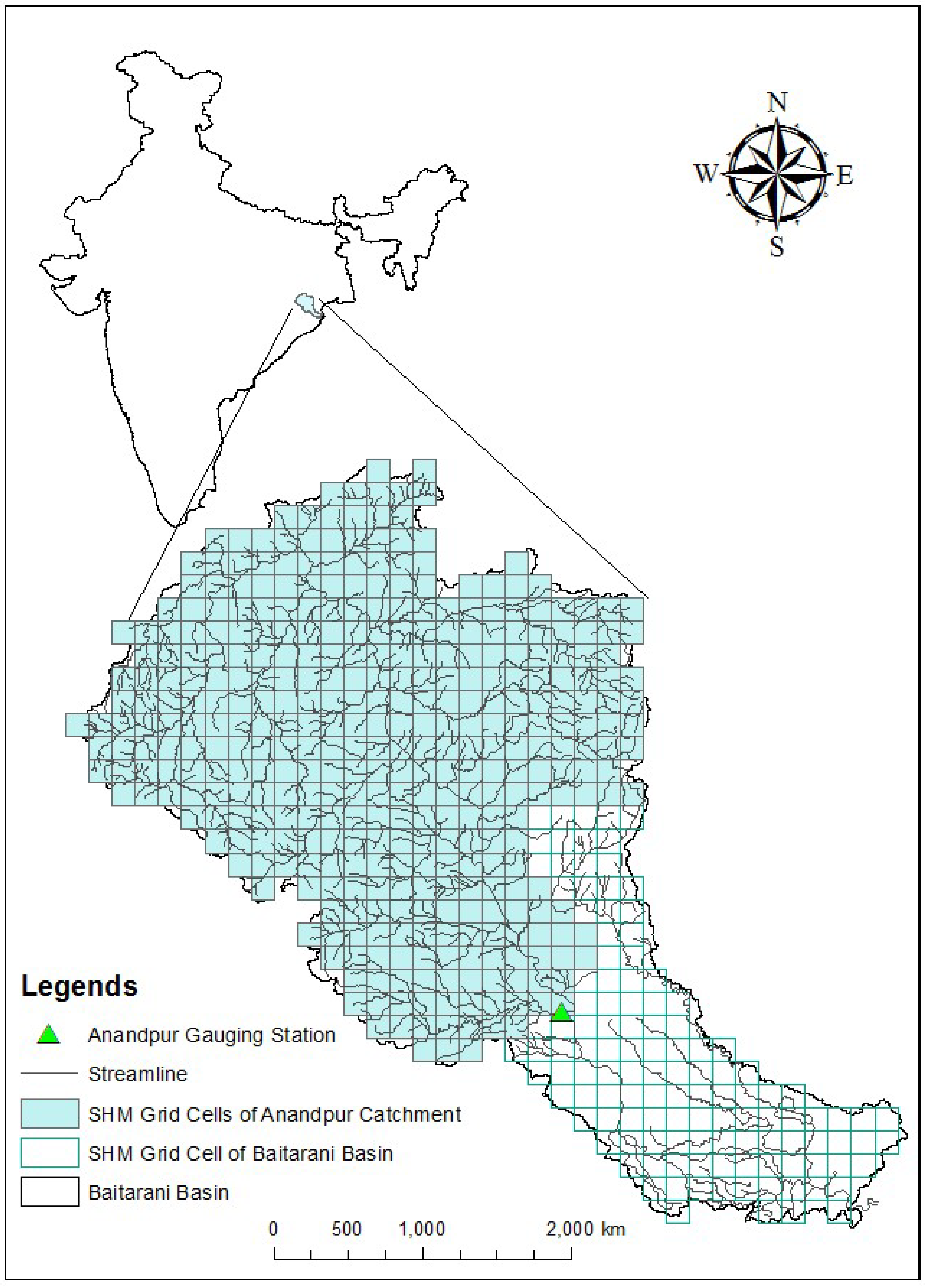
The study has been performed in Baitarani river basin (12,900 km2) in India which is bounded between 20°35′ N to 22°15′ N latitude and 85°10′ E to 87°03′ E longitude (Figure 1). It comes within the sub-tropical monsoon climate zone [38] and receives an annual rainfall of about 1450 mm (Annual Report, 2011-12, 2011). Almost 80% of the annual rainfall occurs during the four months of south-west monsoon season (June to September) that generates heavy flow and creates floods in lower reaches [39]. Daily temperature varies from 5 °C to 47.5 °C. The elevation of the basin ranges from 10 m to 750 m above mean sea level. Soils of this area vary from rich red loamy to gravely detritus.
For a consistent comparison of performances, the same datasets were used in SHM and SWAT models. Daily Rainfall and daily maximum and minimum temperature have been obtained from the India Meteorological Department (IMD), Pune at 1° × 1° resolution. Data have been interpolated to 5 km × 5 km resolution by using bi-linear interpolation technique to use as input into the SHM. Soil and land use land cover (LULC) maps were collected from the Food and Agriculture Organization (FAO) website (http://www.fao.org/soils-portal/soil-survey/soil-maps-and-databases/harmonized-world-soil-database-v12/en/) at 1 km × 1 km scale. The digital elevation model (DEM) of 30 m × 30 m resolution was taken from the Advanced Spaceborne Thermal Emission and Reflection Radiometer (ASTER) website (https://asterweb.jpl.nasa.gov/gdem.asp). All the static information (soil map, LULC map, and DEM) have been resampled into 5 km × 5 km resolution to use in the SHM. The weather database of SWAT is developed using the weather generator (WXGEN) model using the closest station scheme [40]. Observed streamflow data, at Anandpur gauging station (21.21° N, 86.12° E), were collected for the period of 1977 to 2004 from the Central Water Commission (CWC), Bhubaneswar, India.
3. Comparative Discussion on SHM and SWAT
In this section, short descriptions of the SHM and SWAT are provided (Section 3.1 and Section 3.2, respectively). Then the identified sensitive parameters of both the models, which have been used to calibrate the models, are discussed in Section 3.3.
3.1. Description of the SHM
The SHM works on 5 km × 5 km spatial grid resolution and properties at the center of a cell are assumed to be the properties of the cell. SHM has five modules: surface water (SW), forest (F), snowmelt (S), groundwater (GW), and routing (ROU). SHM grid cells corresponding to forest and snow land cover are modeled using the F and S modules, respectively; whereas other grid cells are modeled using the SW module.
In the SW module [41,42], the Soil Conservation Service (SCS) curve number (CN) method [43] is used to estimate the surface runoff along with the Hargreaves method [44] to estimate the potential evapotranspiration (PET). Soil moisture is estimated by using the water balance technique. The soil profile is considered as a single-layered zone of 300 mm, and moisture-holding and moisture-transmitting characteristics of the soil layer and underlying layer are considered to account for the soil moisture. Infiltrated water wets the soil layer, and excess water from the maximum capacity (saturation) contributes after percolation to GW module. The soil moisture is depleted by evapotranspiration, at a potential rate or actual rate, depending on soil moisture condition.
The F module serves, based on water balancing and the dynamics of the subsurface, to provide output in the form of runoff, soil moisture, evapotranspiration, and contribution to groundwater using the technique and parameters stated in [45]. Subsurface is reckoned on having soil matrix and macropores of main bypass and internal catchment types. The main bypass directly contributes to groundwater. Soil matrix is considered of having three layers, which are important with respect to water balance and change in soil moisture. After infiltration, the saturation of three layers gets started from the top in batch, and after complete saturation of the three layers, the excess water goes to groundwater. After a precipitation event, runoff generation occurs according to the antecedent moisture conditions in the subsurface.
The S module determines the snow density from snow albedo [46] for estimating snowmelt depth by using two different algorithms, viz., the temperature index algorithm and radiation-temperature index algorithm. Since the study area does not have any snow land cover; the S module is not considered in this study.
The GW module uses the contribution from SW, F, and S modules and generates baseflow following the water level variation process described in [47]. The resultant baseflow along with the surface runoff generated from other modules is routed up to the outlet as streamflow.
In SHM, a distributed routing technique [41], termed as time-variant spatially distributed direct hydrograph (SDDH) travel time method [48], was adopted. It requires the flow path, which is derived from DEM. The downstream cell, in the direction of the steepest descent, is defined from the DEM by the use of the flow direction geographic information system (GIS) function with a unique connection from each cell to the watershed outlet. This process produces a cell network to present the flow paths. The threshold number of upstream cells is set equal to two (based on trial and error) to delineate the channel network for the watershed. Any cell with a number of upstream draining cells equal to or greater than the threshold value is considered to be a channel cell, whereas others are considered as overland flow cells. The key point of this approach is the travel time estimation. SHM uses MySQL (open source software) as a relational database management system (RDBMS).
3.2. Description of SWAT
SWAT is used for simulation of the water cycle and its corresponding fluxes of energy and matter (e.g., sediment, nutrients, pesticides, and bacteria) as well as the impact of management practices on these fluxes at basin scale [49]. SWAT uses Microsoft Access as RDBMS. SWAT, however, first discretizes the watershed into a network of irregular sub-basins and then divides each sub-basin into HRUs. The model includes components for hydrology, sedimentation, crop growth, nutrients, and agricultural management [11]. A detailed description of all components of the model can be found in Arnold et al. [49] and Neitsch et al. [10].
In the present study, SWAT has been used with the Soil Conservation Service Curve Number (SCS-CN) method as a runoff generation technique along with the Hargreaves method to determine PET. SWAT calculates baseflow contribution to streamflow from groundwater depending on the water balance approach in a shallow aquifer [49]. In SWAT, runoff is first computed separately for each of the HRUs within the sub-basin and then routed through the stream network to obtain the total streamflow for the watershed. Since the study area does not have snow-covered land, the snow-melt runoff simulation procedure of SWAT is not discussed here.
3.3. Sensitive Parameters of Both the Models Used for Calibration
The total number of parameters of the two models varies in number for streamflow analysis. Three parameters of SHM and seven parameters of SWAT have been found sensitive for streamflow simulation (Table 1), in this study.
During calibration of SHM, parameters of SW and ROU modules have been changed manually (since an auto-calibration option is not available). For this purpose CN, Manning’s roughness coefficient for overland cell (no), and Manning’s roughness coefficient for channel cell (nc) have been used as sensitive parameters [50]. The parameters of the F and GW modules have been set at their default values as recommended by the developers. The theoretical ranges of sensitive parameters are given in Table 1. CN is responsible for runoff generation in the SW module, and no and nc affect the routing procedure of generated runoff and baseflow from a grid cell up to the outlet of a basin. Using calibrated values of the sensitive parameters, SHM simulates monthly streamflow at Anandpur gauging station of Baitarani basin.
For the SWAT model, seven sensitive parameters are identified (Table 1) for model calibration based on the analysis of parameter sensitivity using the Latin hypercube-one factor at a time (LH-OAT) method [51]. Curve number (Cn2) and baseflow recession constant (Alpha_bf) are responsible for runoff generation; delay time for aquifer recharge (Gw_delay) and threshold water level in a shallow aquifer for base flow (Gwqmn) are responsible for baseflow generation, and the soil evaporation compensation coefficient (Esco) is responsible for soil evaporation losses. Manning’s n for the main channel (Ch_N2) and Effective hydraulic conductivity of soil (Ch_K2) are responsible for controlling river flow routing. Table 1 summarizes the sensitive parameters of both the models with corresponding hydrological processes, estimation methodology and their theoretical ranges. The table also focuses on the spatial variability of the sensitive parameters.
4. Methodology
4.1. Model Setup, Calibration, Validation
At first, both the models were setup with the same input data. For SHM setup, the Baitarani basin is represented by 498 grid cells of 25 km2. The threshold values of LULC, soil, and slope were taken, respectively, 1%, 1%, and 2% for the development of HRUs in the SWAT model so that the average area of HRUs is around 25 km2 and two discretization schemes come in a balanced scale. This assumption led to having 312 sub-basins and 511 HRUs in the Baitarani basin. However, the smallest HRU has an area of 1.9 km2, and the largest HRU has an area of 52 km2 with an average area of 25.2 km2. Both the models were then calibrated (1977–1990) and validated (1991–2004) on a monthly basis. The performance evaluation of both the models has been done by comparing observed and simulated streamflows by using graphical interpretation and statistical indices, namely coefficient of determination (R2), Nash–Sutcliffe efficiency (NSE), and percent bias (PBIAS) for the calibration and validation periods, separately. The used statistical analyses are discussed below.
4.1.1. Nash Sutcliffe Efficiency (NSE)
It is defined as one minus the sum of the absolute squared differences between observed and simulated values normalized by the variance of observed values [53]. It varies from −∞ to 1, 1 being the perfect fit. It is chosen because of its extensive use in the field of hydrology, which facilitates comparison between different studies. However, it is highly sensitive to peak flows resulting in negligence of low flows.
4.1.2. Coefficient of Determination (R2)
The coefficient of determination (R2) describes the proportion of the total variance in the observed data that can be explained by a model. It ranges from 0 to 1, with higher values indicating better agreement, and is given by:
where, is the average simulated value of streamflow.
4.1.3. Percent Bias (PBIAS)
It measures the average tendency of the simulated data to be larger or smaller than their observed counterparts. Its ideal value is 0. A positive value indicates model underestimation bias and a negative value indicates model overestimation bias.
4.2. Analysis of Results
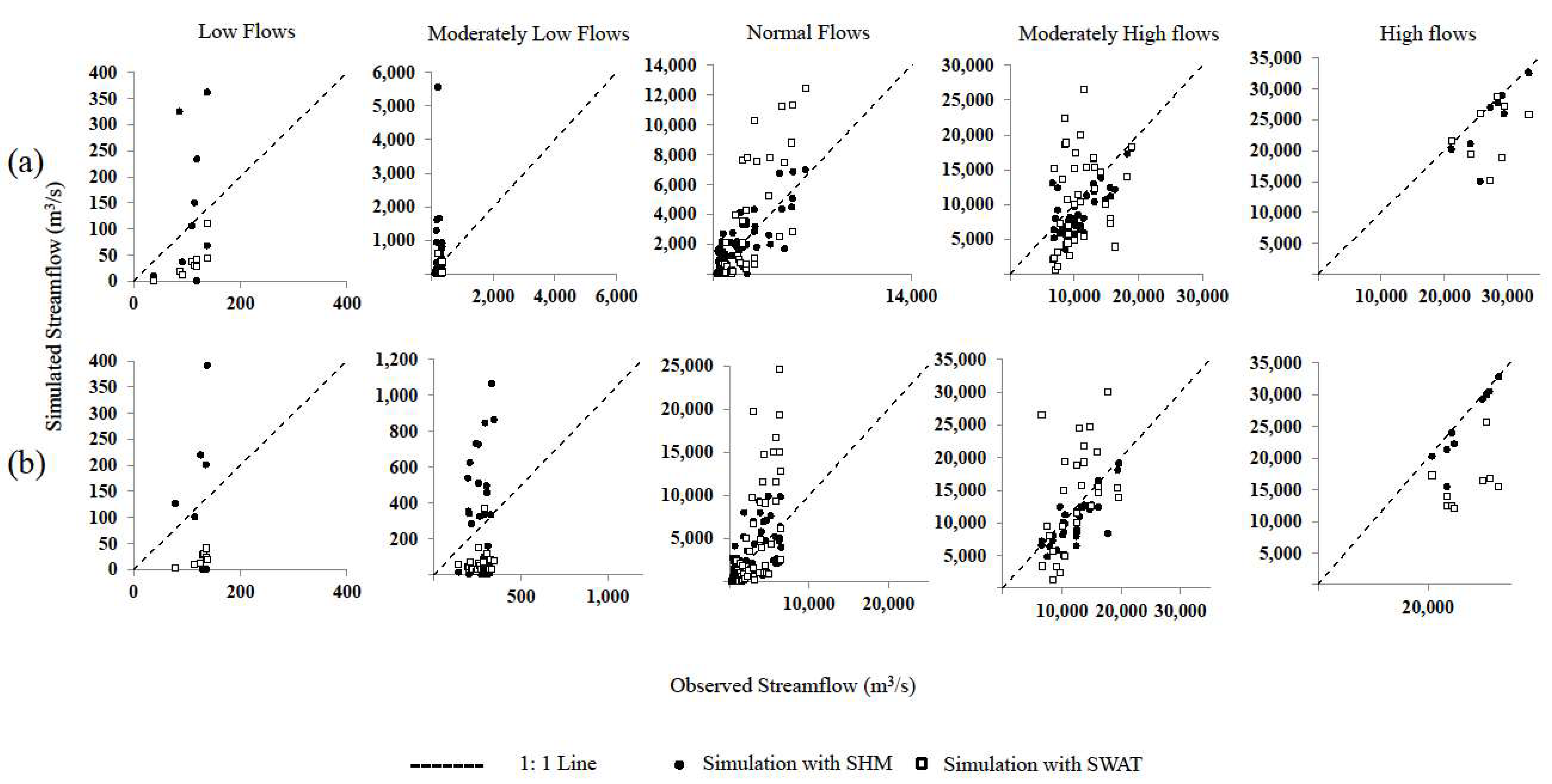
After calibration and validation, the model-simulated streamflows were analyzed to compare model performances for both the periods with respect to annual peaks. Then, inter-annual variability of simulations of both the models for each month of the year, for the total period of analysis, were analyzed. Eventually, the capability of both models was compared using the five percentile series derived from observed data. Therefore, to understand the difference in the capability of the models to simulate different streamflow ranges in an improved manner, four percentile points of observed monthly streamflow, S5 (5th percentile), S25 (25th percentile), S75 (75th percentile), and S95 (95th percentile), were used to divide the overall flow range into five percentile series: low flows (<S5: <139.95 m3/s), moderately low flows (S5–S25: 139.95 m3/s to <349.4 m3/s), normal flows (S25–S75: 349.4 m3/s to <6590 m3/s), moderately high flows (S75–S95: 6590 m3/s to <20,760 m3/s), and high flows (≥S95: ≥20,760 m3/s). Finally, uncertainty analysis has been performed of the models.
Uncertainty Analysis
Using quantile regression, a stochastic approach [54], uncertainty from all sources was analyzed, as a whole and for monthly simulation of both the models at Anandpur gauging station for both the calibration and validation periods. The observed, simulated, and residual values of streamflow are linked with the following equation:
where Q(t) is the observed daily streamflow, is the simulated streamflow, and e(t) is the residual.
The method assumes a functional relationship between residuals and estimates in the Gaussian domain, i.e., normalized quantile streamflow (NQS) and normalized quantile residual (NQR). A linear relation between NQS and NQR was also used in previous studies [55,56]. Hence, NQR may be expressed as:
NQR = a × NQS + b
Different quantile regression lines may be obtained by minimizing the absolute bias by assigning different weights to positive and negative residuals in the Gaussian domain. Absolute bias can be considered for this purpose as an objective function (OF) which is expressed mathematically as:
where is the slope, b is the intercept, and is the quantile regression function which pushes the regression line to the desired location.
To estimate the streamflow corresponding to a given confidence limit, the simulated streamflow is transformed to the Gaussian domain as NQS first, and then, the error in the Gaussian domain, NQR is estimated using the regression line (Equation (5)). The estimated error, NQR is transformed back to the original domain using the pre-estimated mean and standard deviation of the residual. Finally, the estimated residual is added to the daily simulated streamflow to obtain the streamflow which includes uncertainty. Regression lines were used to analyze uncertainty in the simulated streamflow for different confidence intervals. The slope and intercept of these lines are estimated by Equation (6) using the calibration period data. Furthermore, to verify the correctness of error models, the models were applied for both the calibration and validation periods.
Moreover, to have quantitative realization of uncertainty, P and R values have been calculated, and P vs. R plot has been generated for both the calibration and validation periods.
P-value represents the measured data bracketed by the 95 percent predictive uncertainty (PPU) band [57]. P-value has been determined by the following equation:
where, are the total number of observed data points bracketed by the 95PPU band, N is the total number of observed data points.
R-value expresses the relative length of the 95PPU band with respect to the model simulated values [57]. R-value has been determined by the following equation:
where is the standard deviation of the model simulation x. is the average distance between the upper and lower limit of the 95PPU band. has been calculated using the following equation:
where l is counter, k is the total number of simulated data points for streamflow q, and are the upper and lower limit of the 95PPU band.
Both the values vary between 0 and 1. P-value equal to 1 and R-value 0 represent the best model simulation with no uncertainty. In the P-Q plot, this point can be identified as the point of no uncertainty. Since to reach the point of no uncertainty is nearly impossible to achieve for any model simulation as a result of model uncertainties and measurement errors, the simulation nearest to the point may be considered as the simulation with the lowest uncertainty.
5. Results and Discussion
5.1. Calibration and Validation of the Models
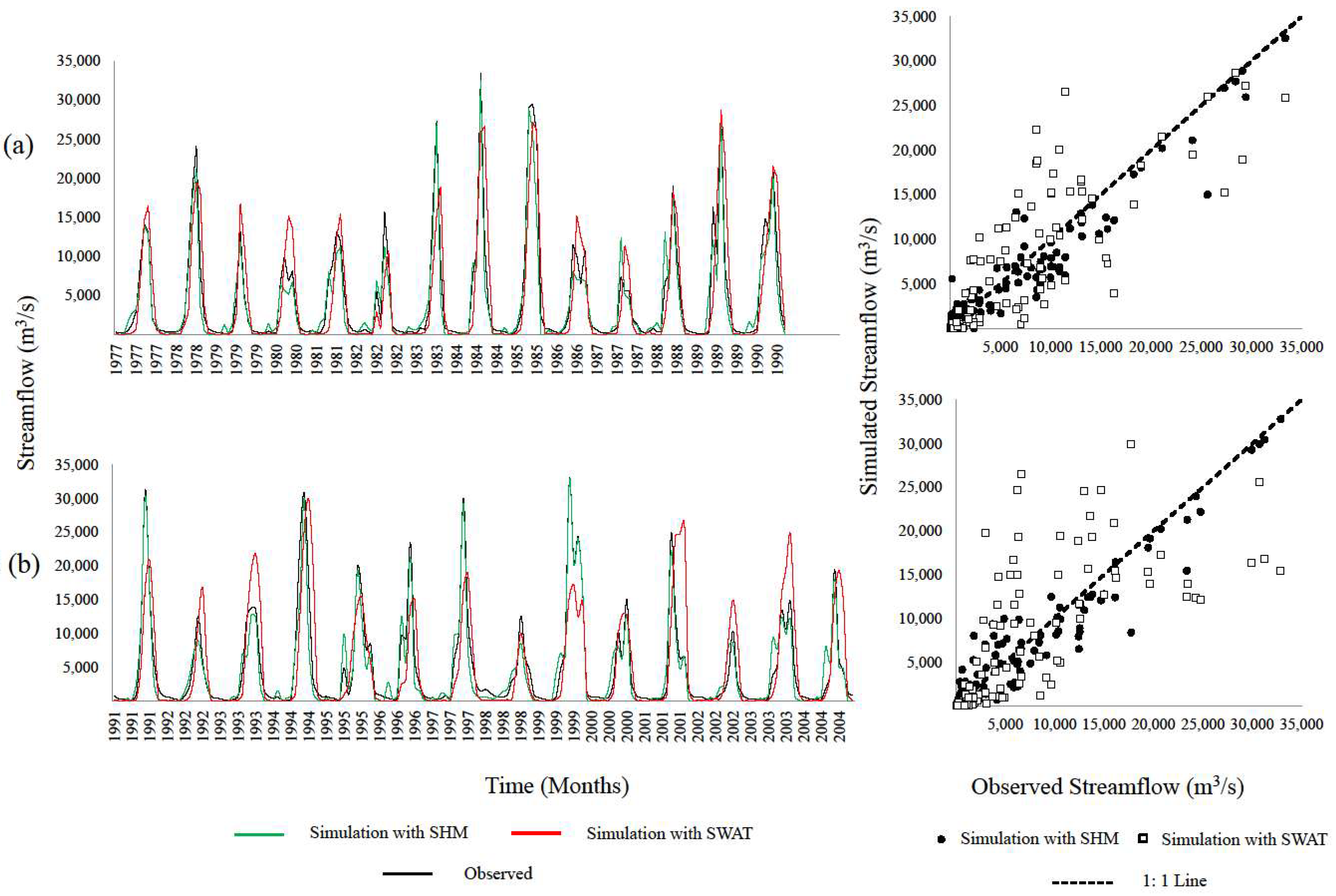
Comparison between observed and models’ simulated monthly streamflow are shown in Figure 2a for the calibration period and in Figure 2b for the validation period. Figures show good agreement among observed and simulated streamflow by both the models. However, SHM simulates the temporal pattern of observed streamflow relatively better in comparison to the SWAT model in both calibration and validation periods including the reproduction of peak flows. To strengthen this observation 1:1 scatter plots, between observed and models’ simulations for the calibration and validation periods, have also been used (shown in Figure 2a,b). From the scatter plots it is evident that SWAT simulated streamflow deviates considerably from the observed streamflow with respect to the SHM simulated counterpart during both the calibration and validation periods. Moreover, scatter plots also depict that SWAT underestimates high flow more in comparison to SHM.
The goodness-of-fit statistics of both the models on monthly calibration and validation are shown in Table 2. Generally, if R2 > 0.6, NSE > 0.5, and −25% ≤ PBIAS ≤ 25%, the model simulation results are judged as satisfactory [58,59]. Thus, both SHM and SWAT models have produced satisfactory model simulations for both the calibration and validation periods in the study area. However, the monthly streamflow simulated by SHM shows better fit with the observed monthly flow in comparison to the SWAT simulated streamflow during the calibration as well as validation periods. SHM shows similarity in results during both the calibration and validation periods with a slightly reduced PBIAS during validation than calibration period, thus, improvement in water balance dynamics. On the other hand, SWAT shows considerable deterioration in results during the validation period in comparison to the calibration period which is evident from the values of R2 and NSE (Table 2). The results, thus, show improved performances of both SHM and SWAT simulations in comparison to previous studies performed at the Anandpur sub-basin [60,61,62,63,64,65].
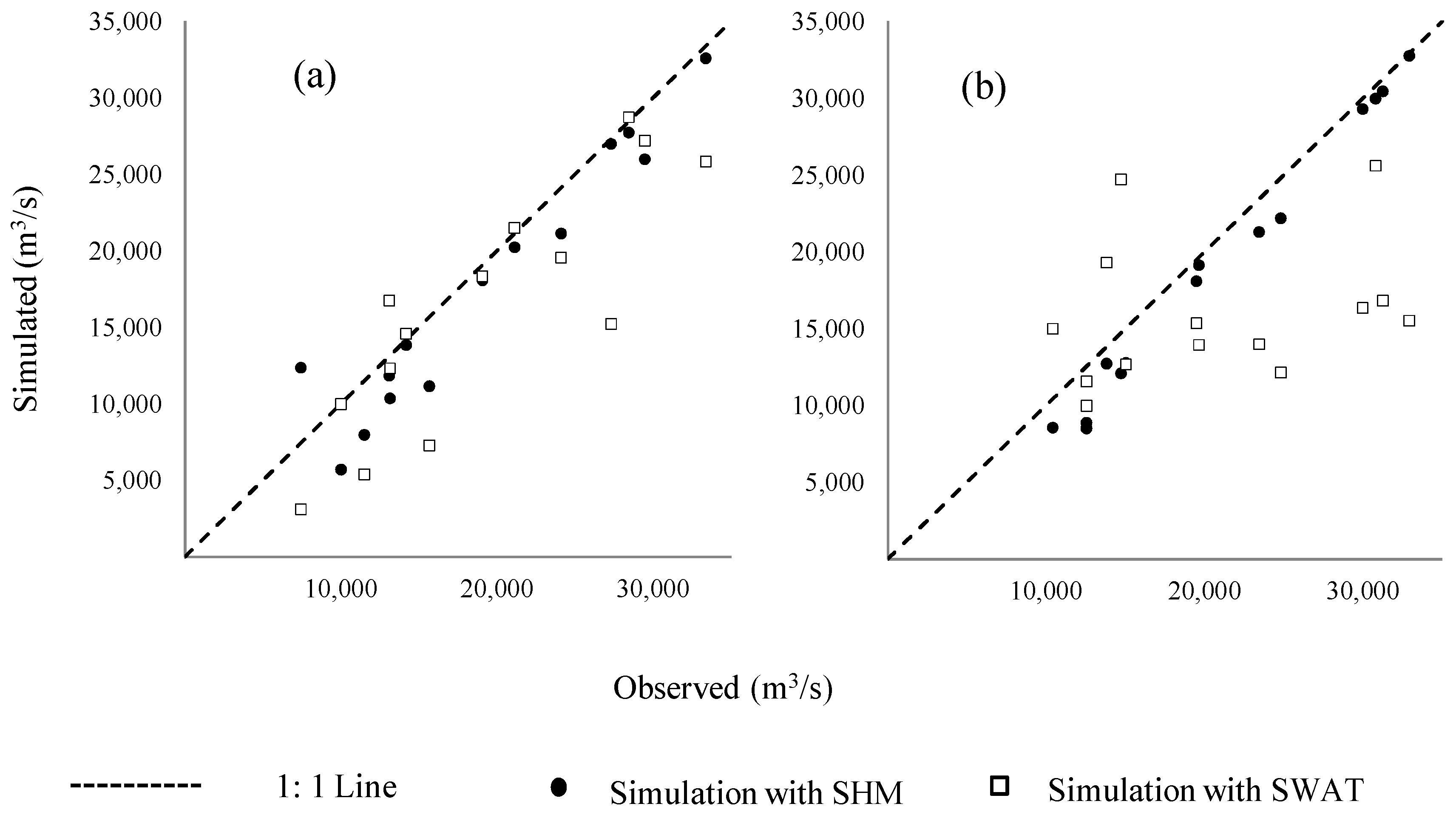
5.2. Analysis to Compare Annual Peaks
To perform comparison of the annual peak simulation capabilities of both the models, observed and simulated annual peaks (from both the models) for the calibration (Figure 3a) and validation (Figure 3b) periods have been plotted against the 1:1 line. Figure 3 depicts that SHM reproduces annual peaks better than SWAT. Therefore, SHM can be a good option for streamflow simulation for extreme rainfall events as well as analyzing flooding possibility in the region. Findings are well comparable with the study performed by Baratti et al. [66] in which they estimated annual flood frequency for the same region.
5.3. Inter-Annual Variability of Model Simulations
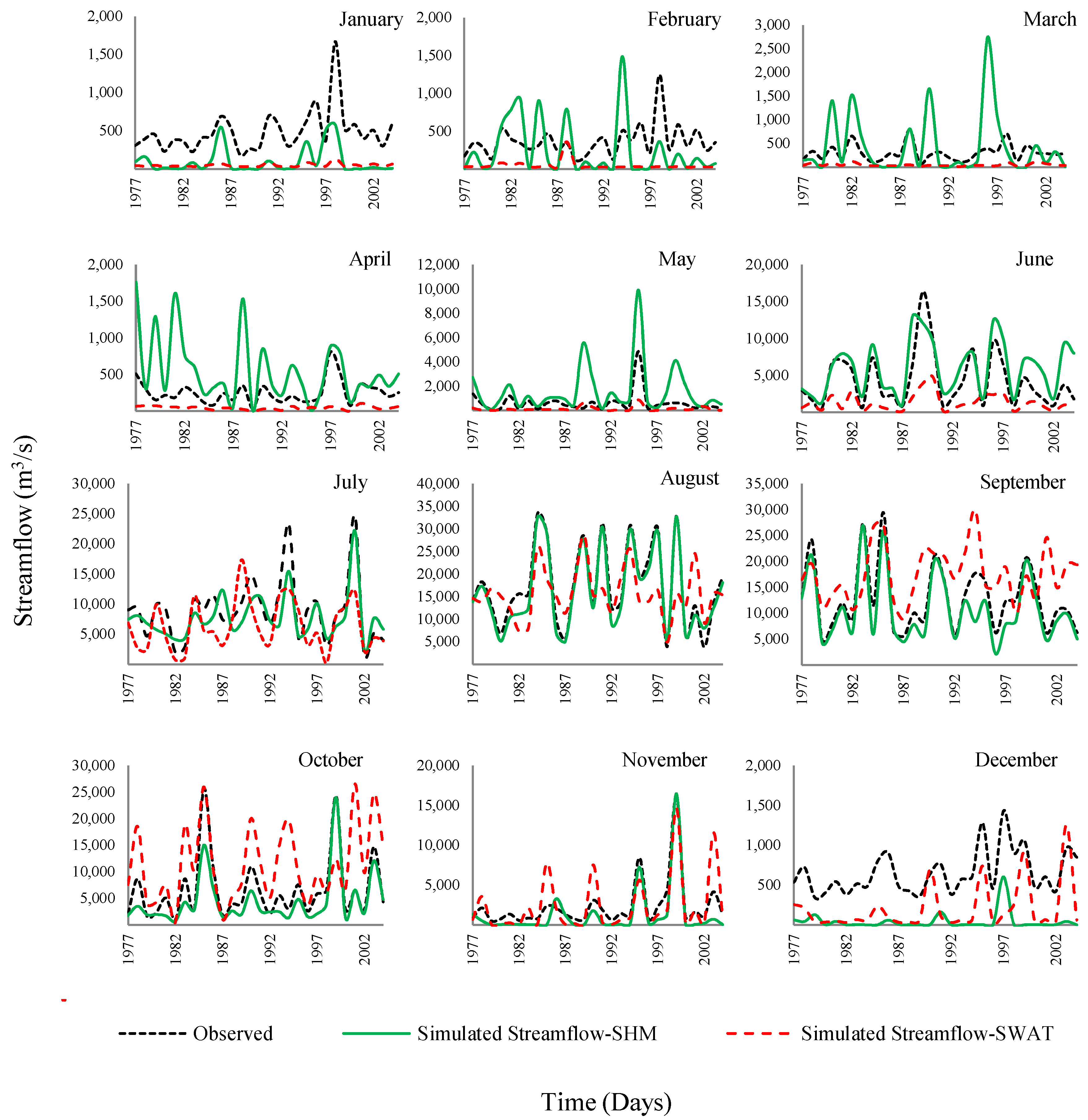
To understand the difference in models’ capabilities of producing inter-annual variability of monthly streamflow, comparison between observed and simulated monthly streamflow from both the models have been analyzed and are shown in Figure 4. From the figure, it is evident that SHM performs satisfactorily in simulating streamflow during the months of June to October (monsoon) season with the best simulation identified for the month of August throughout the analysis period. In addition, it is also evident that SHM reproduces observed streamflow better for all the months over the analysis period in comparison to SWAT streamflow.
The differences in the results of two models for inter-annual variability on a monthly scale for the total period of analysis is mainly attributable to two reasons: different input data interpolation schemes and variation in modeling processes. First, meteorological data have been bi-linearly interpolated into 5 km × 5 km to run SHM and SWAT model and have used the meteorological data from the closest IMD grid to simulate monthly streamflow in a sub-basin instead of interpolation [67] (as stated earlier in Section 2). Different input data interpolation schemes and variation in spatial discretization create the difference in the spatial distribution of meteorological input for the models [30]. Second, apart from SCS-CN of the SW module, no modeling process of SHM matches with the SWAT model. However, the modeling process combination of SHM proved to be better in monsoonal months in comparison to SWAT; though modeling processes of both models may require improvement for the low rainfall months. In particular, water level variation approach of baseflow generation, in SHM, and water balance approach of baseflow calculation, in SWAT, may be compared with separate analysis for the non-monsoonal months, for the purpose. Furthermore, better calibration may also improve results for months with low rainfall.
5.4. Comparison of Model Simulations for Percentile Flows
The models’ performance has also been analyzed in simulating streamflow of various magnitudes by considering five percentile classes (Section 4.2). The respective simulated flows by both models have been compared with that of observed streamflow by using scatter plots for the calibration (Figure 5a) and validation periods (Figure 5b). The performance of SWAT in simulating moderately low flows during the calibration period is better than simulating other streamflow percentiles during both the calibration and validation periods. SHM performs better for simulating normal, moderately high, and high flows during both the calibration and validation periods. Overall, both the models show an extremely poor performance in simulating low flows during both the periods and moderately low flows during the validation period.
The variation in percentile flow estimation of the models can also be attributable to different input data interpolation schemes. However, SCS-CN plays a major role in both models. Therefore, streamflow simulation may not be appropriate when the rainfall amount is small [30,49,68]. Similar results have been identified for the non-monsoonal months during analysis of inter-annual variability of the models, in the previous section. In addition, the different runoff generation technique of the F module and baseflow generation technique of the GW module of SHM (stated earlier in Section 3.1) with respect to techniques used in the SWAT model are also responsible for the different results of the months. In particular, the soil matrix and antecedent condition of the F module may play a role in the poor model simulation of SHM for low and moderate low flows. Moreover, the routing technique of SHM seems to be the reason behind the upper hand in simulating high flows in comparison to SWAT, by capturing the travel time of the streamflow in a better manner.
5.5. Uncertainty Analysis of Monthly Simulations
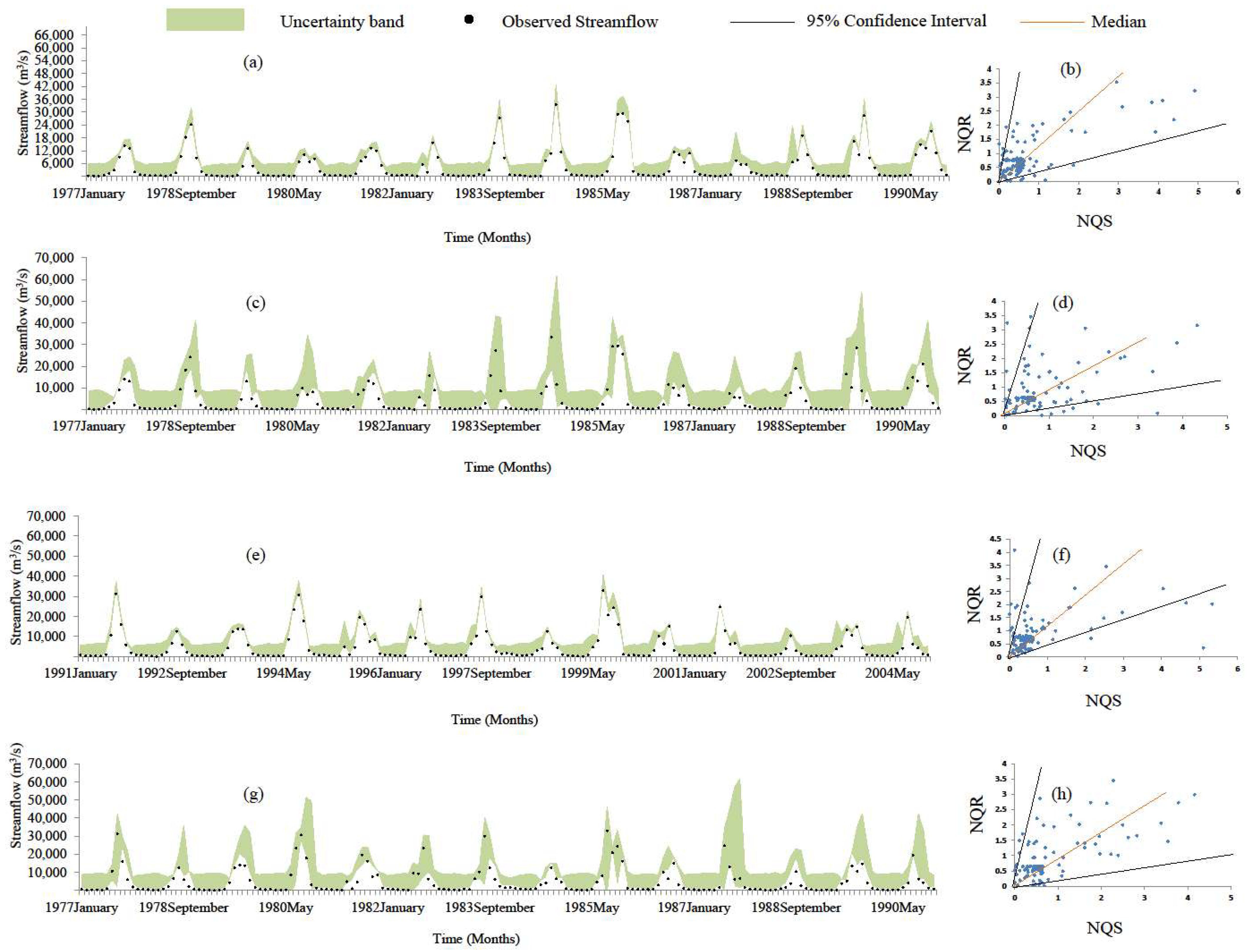
Figure 6a,c present the 95PPU uncertainty band for monthly simulation during the calibration period. Figure 6e,g present the 95PPU uncertainty band for monthly simulation during the validation period. Among them Figure 6a,e are for SHM simulations and Figure 6c,g are for SWAT simulations. In addition, Figure 6b,d present the scatter plot of NQR and NQS along with two regression lines: corresponding to upper and lower limits of 95% confidence interval (CI) and one corresponding to the median for the calibration period. Figure 6b,d are for the SHM and SWAT simulation, respectively. Figure 6f,h present the scatter plot of NQR and NQS along with two regression lines: corresponding to upper and lower limits of 95% confidence interval (CI) and one corresponding to the median for the validation period. Figure 6f,h are for SHM and SWAT simulation, respectively.
Figure 6a,c,e,g depict that most of the observed streamflow falls inside the defined bands, though the amount is higher for SHM simulations (Figure 6a,c). Moreover, from Figure 6a,c,e,g it is also evident that the width of 95PPU band is thinner for SHM simulations in comparison to SWAT simulations. Thus, it can be inferred that SHM has less uncertainty in model simulations in comparison to SWAT simulations. Figure 6b,d,f,h depict the relationship between residual and simulated streamflow in the Gaussian domain and confirm that the simulated streamflow is able to capture 95% of the observed streamflow during the calibration and validation periods for both the models. For estimating the collective uncertainty, Dogulu et al. [69] supported the use of the quantile regression (QR) technique due to its simplicity and linearity which has been used elaborately by Kumar et al. [70].
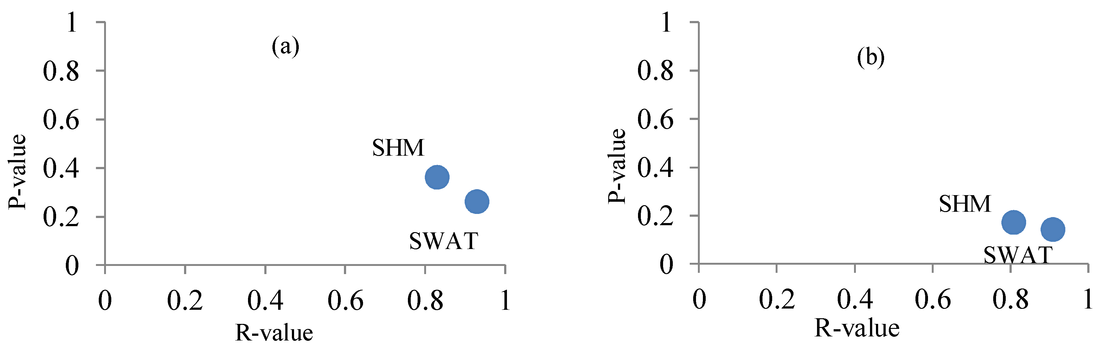
P and R values based on the uncertainty analysis results of SHM and SWAT simulations for the calibration and validation periods, respectively shown in Figure 7a,b, elaborate that SHM poses less uncertainty in monthly simulation than SWAT model.
Though uncertainties from all sources have been counted in the QR uncertainty analysis technique, spatial distributions of input data are different for the models due to different data interpolation techniques and model structures of the two models. Although the models’ parameters take care of the modeling processes during calibration, the spatial variation of input data may affect the uncertainty of the models’ simulation significantly. The results of the uncertainty analysis also represent this aspect and show that SHM represents the spatial variations of landscape characteristics and input data more accurately.
6. Conclusions
SHM and SWAT models were used to simulate the monthly streamflow at Anandpur gauging station of Baitarani basin for in-depth inter-comparison of the models’ performances. The SWAT model was set to have an average size of the HRUs equal to 25.2 km2, (nearly equal to the grid cell resolution of SHM, i.e., 25 km2) so that the two discretization schemes were in similar scale. Results showed that although both SHM and SWAT have produced reasonable results, SHM performed better. To be more specific, SHM performed better in simulating annual peak flows, and reproduced the annual variability of observed streamflow for every month of the year. In addition, SHM estimates normal, moderately high, and high flows better than SWAT. Uncertainty analysis of simulated streamflow of both the models also supports the superiority of SHM model in comparison with SWAT model. Possible impacts of the model structure were also identified for the results.
In summary, SHM produced better results in comparison to SWAT at the monthly scale with proof of better model structure for the large research catchment. However, we cannot draw a conclusion that grid-based hydrological modeling is better than the HRU based. More researches should be carried out for comparing different discretization schemes for other Indian basins and other parts of the world.
Author Contributions
Conceptualization, Y.Z. and P.K.P.; methodology, P.K.P.; software, P.K.P.; validation, P.K.P.; formal analysis, P.K.P.; investigation, P.K.P.; resources, R.S.; data curation, P.K.P.; writing—original draft preparation, P.K.P.; writing—review and editing, Y.Z. and A.M.; visualization, Y.Z.; supervision, A.M., N.P., R.S. and Y.Z.; project administration, R.S.; funding acquisition, Y.Z.
Funding
This research was funded by Space Application Centre (SAC), Ahmedabad, grant number IIT/SRIC/AGFE/DWI/2013-14/124 and the APC was funded by the CAS Pioneer Hundred Talents Program.
Acknowledgments
This work is financially supported by the CAS Pioneer Hundred Talents Program, Space Application Centre (SAC), Ahmedabad (Grant no. IIT/SRIC/AGFE/DWI/2013-14/124). The technical support of programmer Partha Samanta in developing the model is acknowledged. We also acknowledge the technical support of R.P. Singh and P.K. Gupta from SAC, Ahmedabad, and our other project partners from NERIST, Itanagar, IIT Guwahati and IISc, Bangalore.
Conflicts of Interest
The authors declare no conflict of interest.
References
- Liang, X.; Guo, J.; Leung, L.R. Assessment of the effects of spatial resolutions on daily water flux simulations. J. Hydrol. 2004, 298, 287–310. [Google Scholar] [CrossRef]
- Kampf, S.K.; Burges, S.J. A framework for classifying and comparing distributed hillslope and catchment hydrologic models. Water Resour. Res. 2007, 43. [Google Scholar] [CrossRef] [Green Version]
- Khakbaz, B.; Imam, B.; Hsu, K.; Sorooshian, S. From lumped to distributed via semi-distributed: Calibration strategies for semi-distributed hydrologic models. J. Hydrol. 2012, 418–419, 61–77. [Google Scholar] [CrossRef]
- Smith, M.B.; Gupta, H.V. The Distributed Model Intercomparison Project (DMIP)—Phase 2 experiments in the Oklahoma region, USA. J. Hydrol. 2012, 418–419, 1–2. [Google Scholar] [CrossRef]
- Wood, E.F.; Sivapalan, M.; Beven, K.; Band, L. Effects of spatial variability and scale with implications to hydrologic modeling. J. Hydrol. 1988, 102, 29–47. [Google Scholar] [CrossRef]
- Kouwen, N.; Soulis, E.D.; Pietroniro, A.; Donald, J.; Harrington, R.A. Grouped response units for distributed hydrologic modelling. J. Water Resour. Plan. Manag. 1993, 119, 289–305. [Google Scholar] [CrossRef]
- Reggiani, P.; Sivapalan, M.; Majid Hassanizadeh, S. A unifying framework for watershed thermodynamics: Balance equations for mass, momentum, energy and entropy, and the second law of thermodynamics. Adv. Water Resour. 1998, 22, 367–398. [Google Scholar] [CrossRef]
- Winter, T.C. The concept of hydrologic landscapes. J. Am. Water Resour. Assoc. 2001, 37, 335–349. [Google Scholar] [CrossRef]
- Vivoni, E.R.; Ivanov, V.Y.; Bras, R.L.; Entekhabi, D. Generation of triangulated irregular networks based on hydrological similarity. J. Hydrol. Eng. 2004, 9, 288–302. [Google Scholar] [CrossRef]
- Neitsch, S.L.; Arnold, J.G.; Kiniry, J.R.; Srinivasan, R.; Williams, J.R. Soil and Water Assessment Tool Theoretical Documentation Version 2009; Texas Water Resources Institute Technical Report 406; Texas A & M University System, College Station: College Station, TX, USA, 2011. [Google Scholar]
- Rathjens, H.; Oppelt, N. SWAT model calibration of a grid-based setup. Adv. Geosci. 2012, 32, 55–61. [Google Scholar] [CrossRef] [Green Version]
- Gassman, P.W.; Reyes, M.R.; Green, C.H.; Arnold, J.G. The Soil and Water Assessment Tool: Historical development, applications, and future research directions. Trans. ASAE 2007, 50, 1211–1250. [Google Scholar] [CrossRef]
- Arnold, J.G.; Allen, P.M.; Volk, M.; Williams, J.R.; Bosch, D.D. Assessment of different representations of spatial variability on SWAT model performance. Trans. ASABE 2010, 53, 1433–1443. [Google Scholar] [CrossRef]
- Reed, S.; Koren, V.; Smith, M.; Zhang, Z.; Moreda, F.; Seo, D.J. Overall distributed model intercomparison project results. J. Hydrol. 2004, 298, 27–60. [Google Scholar] [CrossRef]
- Finnerty, B.D.; Smith, M.B.; Seo, D.J.; Koren, V.; Moglen, G.E. Space-time scale sensitivity of the Sacramento model to radar-gage precipitation inputs. J. Hydrol. 1997, 203, 21–38. [Google Scholar] [CrossRef]
- Wood, E.F.; Lettenmaier, D.; Liang, X.; Nijssen, B.; Wetzel, S.W. Hydrological modeling of continental-scale basins. Annu. Rev. Earth Planet. Sci. 1997, 25, 279–300. [Google Scholar] [CrossRef]
- Kuo, W.-L.; Steenhuis, T.S.; McCulloch, C.E.; Mohler, C.L.; Weinstein, D.A.; DeGloria, S.D.; Swaney, D.P. Effect of grid size on runoff and soil moisture for a variable-source-area hydrology model. Water Resour. Res. 1999, 35, 3419–3428. [Google Scholar] [CrossRef] [Green Version]
- Andersen, J.; Refsgaard, J.C.; Jensen, K.H. Distributed hydrological modelling of the Senegal River BasinModel construction and validation. J. Hydrol. 2001, 247, 200–214. [Google Scholar] [CrossRef]
- Booij, M.J. Impact of climate change on river flooding assessed with different spatial model resolutions. J. Hydrol. 2005, 303, 176–198. [Google Scholar] [CrossRef]
- Orth, R.; Staudinger, M.; Seneviratne, S.I.; Seibert, J.; Zappa, M. Does model performance improve with complexity? A case study with three hydrological models. J. Hydrol. 2015, 523, 147–159. [Google Scholar] [CrossRef] [Green Version]
- Haghnegahdar, A.; Tolson, B.A.; Craig, J.R.; Paya, K.T. Assessing the performance of a semi-distributed hydrological model under various watershed discretization schemes. Hydrol. Process. 2015, 29, 4018–4031. [Google Scholar] [CrossRef]
- Abu El-Nasr, A.; Arnold, J.G.; Feyen, J.; Berlamont, J. Modelling the hydrology of a catchment using a distributed and a semi-distributed model. Hydrol. Process. 2005, 19, 573–587. [Google Scholar] [CrossRef]
- Singh, J.; Knapp, H.V.; Arnold, J.G.; Demissie, M. Hydrological modeling of the Iroquois river watershed using HSPF and SWAT. J. Am. Water Resour. Assoc. 2005, 41, 343–360. [Google Scholar] [CrossRef]
- Im, S.; Brannan, K.M.; Mostaghimi, S.; Kim, S.M. Comparison of HSPF and SWAT models performance for runoff and sediment yield prediction. J. Environ. Sci. Health Part A Toxic/Hazard. Subst. Environ. Eng. 2007, 42, 1561–1570. [Google Scholar] [CrossRef]
- Nasr, A.; Bruen, M.; Jordan, P.; Moles, R.; Kiely, G.; Byrne, P. A comparison of SWAT, HSPF and SHETRAN/GOPC for modelling phosphorus export from three catchments in Ireland. Water Res. 2007, 41, 1065–1073. [Google Scholar] [CrossRef] [Green Version]
- Li, Z.; Xu, Z.; Li, Z. Performance of WASMOD and SWAT on hydrological simulation in Yingluoxia watershed in northwest of China. Hydrol. Process. 2011, 25, 2001–2008. [Google Scholar] [CrossRef]
- Cornelissen, T.; Diekkrüger, B.; Giertz, S. A comparison of hydrological models for assessing the impact of land use and climate change on discharge in a tropical catchment. J. Hydrol. 2013, 498, 221–236. [Google Scholar] [CrossRef]
- Xie, H.; Lian, Y. Uncertainty-based evaluation and comparison of SWAT and HSPF applications to the Illinois River Basin. J. Hydrol. 2013, 481, 119–131. [Google Scholar] [CrossRef]
- Sommerlot, A.R.; Nejadhashemi, A.P.; Woznicki, S.A.; Giri, S.; Prohaska, M.D. Evaluating the capabilities of watershed-scale models in estimating sediment yield at field-scale. J. Environ. Manag. 2013, 127, 228–236. [Google Scholar] [CrossRef]
- Zhang, L.; Jin, X.; He, C.; Zhang, B.; Zhang, X.; Li, J.; Zhao, C.; Tian, J.; DeMarchi, C. Comparison of SWAT and DLBRM for hydrological modeling of a mountainous watershed in arid northwest China. J. Hydrol. Eng. 2016, 21, 4016007. [Google Scholar] [CrossRef]
- Pignotti, G.; Rathjens, H.; Cibin, R.; Chaubey, I.; Crawford, M. Comparative analysis of HRU and grid-based SWAT models. Water 2017, 9, 272. [Google Scholar] [CrossRef]
- Surfleet, C.G.; Tullos, D.; Chang, H.; Jung, I.-W. Selection of hydrologic modeling approaches for climate change assessment: A comparison of model scale and structures. J. Hydrol. 2012, 464–465, 233–248. [Google Scholar] [CrossRef]
- Flügel, W.-A. Combining GIS with regional hydrological modelling using hydrological response units (HRUs): An application from Germany. Math. Comput. Simul. 1997, 43, 297–304. [Google Scholar] [CrossRef]
- Jiang, T.; Chen, Y.D.; Xu, C.Y.; Chen, X.; Chen, X.; Singh, V.P. Comparison of hydrological impacts of climate change simulated by six hydrological models in the Dongjiang Basin, South China. J. Hydrol. 2007, 336, 316–333. [Google Scholar] [CrossRef]
- Najafi, M.R.; Moradkhani, H.; Jung, I.W. Assessing the uncertainties of hydrologic model selection in climate change impact studies. Hydrol. Process. 2011, 25, 2814–2826. [Google Scholar] [CrossRef]
- Singh, V.P. Computer Models of Watershed Hydrology; Water Resources Publications, LLC: Littleton, CO, USA, 1995. [Google Scholar]
- Haverkamp, S.; Srinivasan, R.; Frede, H.G.; Santhi, C. Subwatershed spatial analysis tool: Discretization of a distributed hydrologic model by statistical criteria. J. Am. Water Resour. Assoc. 2002, 38, 1723–1733. [Google Scholar] [CrossRef]
- Dahm, R.J.; Singh, U.K.; Lal, M.; Marchand, M.; Sperna Weiland, F.C.; Singh, S.K.; Singh, M.P. Downscaling GCM data for climate change impact assessments on rainfall: A practical application for the Brahmani-Baitarani river basin. Hydrol. Earth Syst. Sci. Discuss. 2016, 499, 1–42. [Google Scholar] [CrossRef]
- Nayak, P.C.; Sudheer, K.P.; Rangan, D.M.; Ramasastri, K.S. A neuro-fuzzy computing technique for modeling hydrological time series. J. Hydrol. 2004, 291, 52–66. [Google Scholar] [CrossRef]
- Sharpley, A.N.; Williams, J.R. EPIC—Erosion/Productivity Impact Calculator: 1. Model Documentation; USDA Technical Bulletin No. 1768; USDA: Washington, DC, USA, 1990.
- Paul, P.K.; Kumari, N.; Panigrahi, N.; Mishra, A.; Singh, R. Implementation of cell-to-cell routing scheme in a large scale conceptual hydrological model. Environ. Model. Softw. 2018, 101, 23–33. [Google Scholar] [CrossRef]
- Paul, P.K.; Gaur, S.; Yadav, B.; Panigrahy, N.; Mishra, A.; Singh, R. Diagnosing credibility of a large-scale conceptual hydrological model in simulating streamflow. J. Hydrol. Eng. 2019, 24, 4019004. [Google Scholar] [CrossRef]
- Chow, V.T.; Maidment, D.R.; Mays, L.W. Applied Hydrology; McGraw-Hill: New York, NY, USA, 2005; pp. 147–155. [Google Scholar]
- Hargreaves, G.H.; Samani, Z.A. Reference crop evapotranspiration from ambient air temperature. Am. Soc. Agric. Eng. 1985, 1, 96–99. [Google Scholar] [CrossRef]
- Das, P.; Islam, A.; Dutta, S.; Dubey, A.K.; Sarkar, R. Estimation of runoff curve numbers using a physically-based approach of preferential flow modelling. In Hydrology in a Changing World: Environmental and Human Dimensions: Proceedings of the FRIEND-Water 2014; IAHS Publication: Wallingford, Germany, 2014; Volume 363, pp. 443–448. [Google Scholar]
- Smith, J.L.; Halverson, H.G. Estimating Snowpack Density from Albedo Measurement; Research Paper PSW-RP-136; U.S. Department of Agriculture, Forest Service, Pacific Southwest Forest and Range Experiment Station: Portland, OR, USA, 1979.
- Sekhar, M.; Rasmi, S. Groundwater flow modeling of Gundal sub-basin in Kabini river basin, India. Asian J. Water Environ. Pollut. 2004, 1, 65–77. [Google Scholar] [CrossRef]
- Du, J.; Xie, H.; Hu, Y.; Xu, Y.; Xu, C.Y. Development and testing of a new storm runoff routing approach based on time variant spatially distributed travel time method. J. Hydrol. 2009, 369, 44–54. [Google Scholar] [CrossRef]
- Arnold, J.G.; Srinivasan, R.; Muttiah, R.S.; Williams, J.R. Large area hydrologic modeling and assessment Part I: Model development. J. Am. Water Resour. Assoc. 1998, 34, 73–89. [Google Scholar] [CrossRef]
- Indian Institute of Technology Kharagpur. Development of Conceptual Hydrological Model for Different Ecosystems of India; Annual Report; Indian Institute of Technology Kharagpur: West Bengal, India, 2017; pp. 1–19. [Google Scholar]
- Van Griensven, A.; Meixner, T.; Grunwald, S.; Bishop, T.; Diluzio, M.; Srinivasan, R. A global sensitivity analysis tool for the parameters of multi-variable catchment models. J. Hydrol. 2006, 324, 10–23. [Google Scholar] [CrossRef]
- Mockus, V. Estimation of direct runoff from storm rainfall. In SCS National Engineering Handbook; U.S. Department of Agriculture: Washington, DC, USA, 1972; pp. 10.1–10.16. [Google Scholar]
- Nash, J.E.; Sutcliffe, J.V. River flow forecasting through conceptual models part I—A discussion of principles. J. Hydrol. 1970, 10, 282–290. [Google Scholar] [CrossRef]
- Koenker, R.; Bassett, G. Regression Quantiles. Econometrica 1978, 46, 33. [Google Scholar] [CrossRef]
- Koenker, R.; Hallock, K.F. Quantile regression. J. Econ. Perspect. 2001, 15, 143–156. [Google Scholar] [CrossRef]
- Weerts, A.H.; Winsemius, H.C.; Verkade, J.S. Estimation of predictive hydrological uncertainty using quantile regression: Examples from the National Flood Forecasting System (England and Wales). Hydrol. Earth Syst. Sci. 2011, 15, 255–265. [Google Scholar] [CrossRef]
- Xue, C.; Chen, B.; Wu, H. Parameter uncertainty analysis of surface flow and sediment yield in the Huolin Basin, China. J. Hydrol. Eng. 2014, 19, 1224–1236. [Google Scholar] [CrossRef]
- Moriasi, D.N.; Arnold, J.G.; Van Liew, M.W.; Bingner, R.L.; Harmel, R.D.; Veith, T.L. Model evaluation guidelines for systematic quantification of accuracy in watershed simulations. Trans. ASABE 2007, 50, 885–900. [Google Scholar] [CrossRef]
- Moriasi, D.N.; Gitau, M.W.; Pai, N.; Daggupati, P. Hydrologic and water quality models: Performance measures and evaluation criteria. Trans. ASABE 2015, 58, 1763–1785. [Google Scholar] [CrossRef]
- Mujumdar, P.P.; Ghosh, S. Modeling GCM and scenario uncertainty using a possibilistic approach: Application to the Mahanadi River, India. Water Resour. Res. 2008, 44, 1–15. [Google Scholar] [CrossRef]
- Gosain, A.K.; Rao, S.; Arora, A. Climate change impact assessment of water resources of India. Curr. Sci. 2011, 101, 356–371. [Google Scholar]
- Islam, A.; Sikka, A.K.; Saha, B.; Singh, A. Streamflow response to climate change in the Brahmani river basin, India. Water Resour. Manag. 2012, 26, 1409–1424. [Google Scholar] [CrossRef]
- Mitra, S.; Mishra, A. Hydrologic response to climatic change in the Baitarni river basin. J. Indian Water Resour. Soc. 2014, 34, 10. [Google Scholar]
- Paul, P.K.; Mishra, A. Streamflow assessment in changing monsoon climate in two neighbouring river basins of eastern India. J. Indian Water Resour. Soc. 2018, 38, 1–10. [Google Scholar]
- Sindhu, K.; Durga Rao, K.H.V. Hydrological and hydrodynamic modeling for flood damage mitigation in Brahmani–Baitarani river basin, India. Geocarto Int. 2016, 32, 1004–1016. [Google Scholar] [CrossRef]
- Baratti, E.; Montanari, A.; Castellarin, A.; Salinas, J.L.; Viglione, A.; Bezzi, A. Estimating the flood frequency distribution at seasonal and annual time scales. Hydrol. Earth Syst. Sci. 2012, 16, 4651–4660. [Google Scholar] [CrossRef] [Green Version]
- Arnold, J.G.; Fohrer, N. SWAT2000: Current capabilities and research opportunities in applied watershed modelling. Hydrol. Process. 2005, 19, 563–572. [Google Scholar] [CrossRef]
- Mishra, S.K.; Singh, V.P. SCS-CN Method. Soil Conservation Service Curve Number (SCS-CN) Methodology; Mishra, S.K., Singh, V.P., Eds.; Springer: Berlin, Germany, 2003; pp. 84–146. [Google Scholar]
- Dogulu, N.; López López, P.; Solomatine, D.P.; Weerts, A.H.; Shrestha, D.L. Estimation of predictive hydrologic uncertainty using the quantile regression and UNEEC methods and their comparison on contrasting catchments. Hydrol. Earth Syst. Sci. 2015, 19, 3181–3201. [Google Scholar] [CrossRef] [Green Version]
- Kumar, A.; Singh, R.; Jena, P.P.; Chatterjee, C.; Mishra, A. Identification of the best multi-model combination for simulating river discharge. J. Hydrol. 2015, 525, 313–325. [Google Scholar] [CrossRef]
Figure 1.
Index map of Baitarani river basin showing streamline and grid cells of SHM.

Figure 2.
Comparison between observed and simulated monthly streamflow hydrographs and scatter plots during (a) calibration and (b) validation periods.
Figure 2.
Comparison between observed and simulated monthly streamflow hydrographs and scatter plots during (a) calibration and (b) validation periods.

Figure 3.
Comparison between observed and models simulated annual peaks during (a) calibration and (b) validation period.
Figure 3.
Comparison between observed and models simulated annual peaks during (a) calibration and (b) validation period.

Figure 4.
Comparison between observed and simulated monthly streamflow for each month of the year over the total period (calibration and validation) of analysis.
Figure 4.
Comparison between observed and simulated monthly streamflow for each month of the year over the total period (calibration and validation) of analysis.

Figure 5.
Comparison between observed and models’ simulated five streamflow quantile ranges during (a) calibration period and (b) validation period.
Figure 5.
Comparison between observed and models’ simulated five streamflow quantile ranges during (a) calibration period and (b) validation period.

Figure 6.
(a) Observed discharge and uncertainty band for SHM simulation for calibration period, (b) Error model of SHM simulation for calibration period in normalized domain (c) Observed discharge and uncertainty band for SWAT simulation for calibration period, (d) Error model of SWAT simulation for calibration period in normalized domain (e) Observed discharge and uncertainty band for SHM simulation for validation period, (f) Error model of SHM simulation for validation period in normalized domain (g) Observed discharge and uncertainty band for SWAT simulation for validation period, (h) Error model of SWAT simulation for validation period in normalized domain.

Figure 7.
P-value vs. R-value for (a) calibration period and (b) validation period for the SHM and SWAT model simulations.
Figure 7.
P-value vs. R-value for (a) calibration period and (b) validation period for the SHM and SWAT model simulations.


Table 1.
Summary of the sensitive parameters, respective hydrological processes with methodology, theoretical range of their values and information on the spatial variation over the study area, used by SWAT and SHM to simulate hydrological components.
Table 1.
Summary of the sensitive parameters, respective hydrological processes with methodology, theoretical range of their values and information on the spatial variation over the study area, used by SWAT and SHM to simulate hydrological components.
| SWAT | SHM | ||||||||||
|---|---|---|---|---|---|---|---|---|---|---|---|
| List of Sensitive Parameters | Process | Method | Theoretical Range of Parameter Values | Calibrated Range of Parameter Values | Spatially Varied or Not | List of Sensitive Parameters | Process | Method | Theoretical Range of Parameter Values | Calibrated Range of Parameter Values | Spatially Varied or Not |
| Cn2 | Runoff | SCS-CN [52] | 0–100 | 50–100 | Yes | CN | Runoff (SW) | SCS-CN [52] | 0–100 | 30–100 | Yes |
| Gwqmn | Baseflow | Threshold value based contribution from shallow aquifer storage | 0–5000 (mm) | 0–300 | Yes | ||||||
| Gw_delay | 0–500 (day) | 8 | No | ||||||||
| Alpha_bf | 0–1 | 0.5 | Yes | ||||||||
| Ch_N2 | River flow Routing | Variable storage/Muskingum | −0.01–0.03 | 0.03 | No | no | Routing (ROU) | SDDH [48] | 0.01–0.05 | 0.01–0.03 | Yes |
| Ch_K2 | 0–500 (mm/h) | 0.45 | No | nc | 0.01–0.05 | 0.015 | No | ||||
| Esco | To compensate the soil evaporative demand with the depth of soil layers | Water balance | 0–1 | 0.01–0.95 | Yes | ||||||
| Total | 7 | 3 | |||||||||
Enlargements: Cn2 (Curve number), Gwqmn (Threshold water level in shallow aquifer for base flow), Gw_delay (Delay time for aquifer recharge), Alpha_bf (Baseflow recession constant), Ch_N2 (Manning’s n for main channel), Ch_K2 (Effective hydraulic conductivity of soil), Esco (Soil evaporation compensation coefficient), CN (Curve Number), no (Manning’s roughness co-efficient for overland flow), nc (Manning’s roughness co-efficient for channel flow).
Table 2.
Calibration and validation performances of the models at a monthly scale.
| Period | Statistics | SHM | SWAT |
|---|---|---|---|
| Calibration | R2 | 0.93 | 0.75 |
| NSE | 0.92 | 0.72 | |
| PBIAS | 11.62 | 2.01 | |
| Validation | R2 | 0.93 | 0.58 |
| NSE | 0.92 | 0.50 | |
| PBIAS | 8.67 | −1.4 |
© 2019 by the authors. Licensee MDPI, Basel, Switzerland. This article is an open access article distributed under the terms and conditions of the Creative Commons Attribution (CC BY) license (http://creativecommons.org/licenses/by/4.0/).
Share and Cite
MDPI and ACS Style
Paul, P.K.; Zhang, Y.; Mishra, A.; Panigrahy, N.; Singh, R. Comparative Study of Two State-of-the-Art Semi-Distributed Hydrological Models. Water 2019, 11, 871. https://doi.org/10.3390/w11050871
AMA Style
Paul PK, Zhang Y, Mishra A, Panigrahy N, Singh R. Comparative Study of Two State-of-the-Art Semi-Distributed Hydrological Models. Water. 2019; 11(5):871. https://doi.org/10.3390/w11050871
Chicago/Turabian StylePaul, Pranesh Kumar, Yongqiang Zhang, Ashok Mishra, Niranjan Panigrahy, and Rajendra Singh. 2019. "Comparative Study of Two State-of-the-Art Semi-Distributed Hydrological Models" Water 11, no. 5: 871. https://doi.org/10.3390/w11050871
Note that from the first issue of 2016, this journal uses article numbers instead of page numbers. See further details here.