Shock-Capturing Boussinesq Modelling of Broken Wave Characteristics Near a Vertical Seawall


1
Ocean College, Zhejiang University, Zhoushan 316021, China
2
Key Laboratory of Coastal Disasters and Defense of Ministry of Education, Nanjing 210098, China
3
National Marine Hazard Mitigation Service, Ministry of Natural Resources of the People’s Republic of China, Beijing 100000, China
*
Author to whom correspondence should be addressed.
Water 2018, 10(12), 1876; https://doi.org/10.3390/w10121876
Submission received: 1 November 2018
/
Revised: 28 November 2018
/
Accepted: 12 December 2018
/
Published: 19 December 2018
(This article belongs to the Section Hydraulics and Hydrodynamics)
Abstract
:Broken wave characteristics in front of a vertical seawall were modeled and studied using a shock-capturing Boussinesq wave model FUNWAVE-TVD. Validation with the experimental data confirmed the capability of FUNWAVE-TVD in predicting the wave characteristics via the shock-capturing method. Compared to the results obtained from the Boussinesq model coupled with an empirical breaking model, the advantage of the present shock-capturing model for the broken waves near a vertical seawall was clearly revealed. A preliminary investigation of the effects of the key parameters, such as the incident wave height, water level at the seawall, and seabed slope, on the wave kinematics (i.e., the root mean square of the surface fluctuations and depth-averaged horizontal velocity) near the seawall was then conducted through a series of numerical experiments. The numerical results indicate the incident wave height and the water depth at the seawall are the important parameters in determining the magnitude of the wave kinematics, while the effect of the seabed slope seems to be insignificant. The role of the breaking point locations is also highlighted in this study, in which case further breaking can reduce the wave kinematics significantly for the coastal structures predominately subjected to broken waves.
1. Introduction
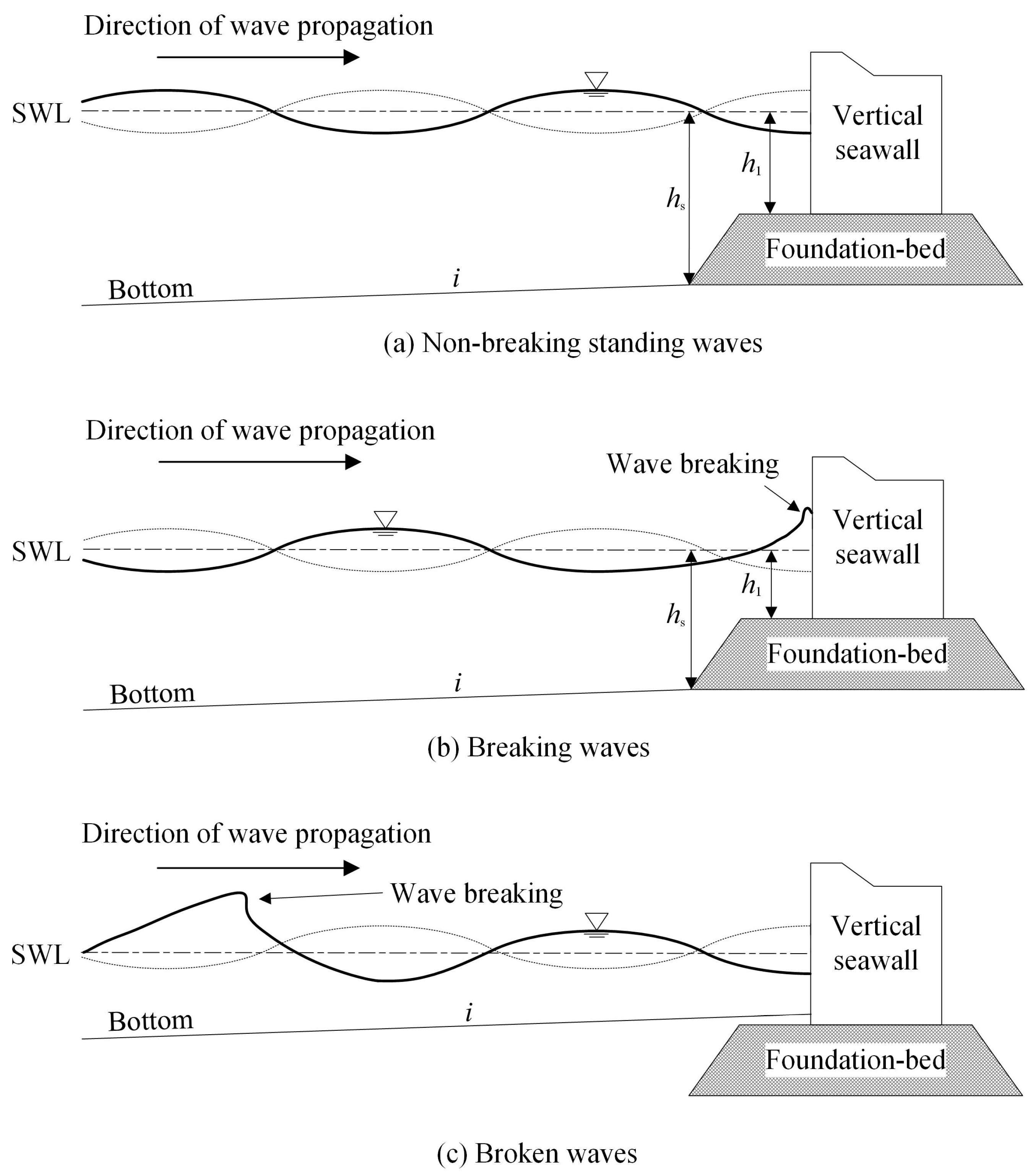
The vertical seawall is one of the most widely-used coastal structures for shore and harbor protections from water wave actions. In general, there are three kinds of wave types forming in front of a vertical seawall, which are non-breaking standing waves, breaking waves and broken waves [1]. The non-breaking standing waves are the waves which do not break in front of a vertical seawall (Figure 1a); the breaking waves are the waves which break above the foundation bed close to the seawall (Figure 1b); the broken waves are the waves which break around antinodes at least a half wavelength from a vertical seawall on the sloping beach and usually form when the foundation bed is low or underground (Figure 1c). Table 1 shows the primary conditions to form these three wave types [1].
Over the decades, numerous experimental and numerical studies have been carried out to investigate the breaking waves in front of vertical seawalls (e.g., [2,3,4,5,6,7,8,9,10]) since they usually reproduce impulsive loads directly on vertical seawalls with a high magnitude. The generation mechanism of impulsive pressure and responses of structures were studied. Several empirical formulations and numerical models were also proposed for the evaluation of breaking wave loadings. Compared to the studies of breaking waves, researches related to the broken waves in front of seawalls are very lacking. The impulsive pressure induced by broken waves tends to be lower than the one induced by breaking waves and therefore, broken waves are not always explicitly treated in the design of vertical seawalls. As more and more protecting vertical seawalls are built along coastlines, where structures are predominately subjected to broken waves, against the increasing risk due to the sea-level rising and storm surges, there is a dawning realization that broken wave loads may endanger the endurance of structures significantly due to their long durations [11]. Moreover, except for the wave loading, broken waves may extend over a broad region and the morphological change, especially the scouring in front of a vertical seawall which can affect the stability of the structure, caused by broken waves is reported to be more serious than that by the other two wave types [1]. Therefore, reliable predictive models and the study of broken wave characteristics near vertical seawalls still have important engineering significance for the design of the seawall subjected to the broken waves.
There are vast ranges of existing models for predictions of nearshore wave hydrodynamics and these models may be mainly classified into three categories. The first category is based on energy balance equations (e.g., [12,13]), which demonstrate reasonable predictive skills of phase-averaged nearshore current field. However, these models are based on the assumptions of linear progressive waves and may not be applied to the wave field where waves have skewed and asymmetric profiles. Moreover, these kinds of models completely fail in modeling waves in front of structures due to the lack of wave reflection mechanism. The second category refers to a number of Computational Fluid Dynamics (CFD) models (e.g., [14,15,16]), which directly solves the Navier–Stokes equations with certain turbulence models. Velocity filed can be directly obtained from these models and wave impact associated with wave-structure interactions can be estimated conveniently. However, these models are computationally expensive so far and may be still limited to small-scale phenomena, such as the breaking waves in front of seawalls.
The third category mainly refers to the depth-integrated Boussinesq-type wave model, which employs a polynomial approximation to the vertical profile of velocity field, reducing the dimensions of a three-dimensional problem by one. This category may be regarded as somewhat between the above-mentioned two categories due to the efficiency and applicability of Boussinesq equations. Over the last decades, considerable efforts (e.g., [17,18,19,20]) have been made to improve the dispersive and nonlinear property of the classical Boussinesq equations [21]. Meanwhile, several empirical sub-models have also been proposed to accommodate wave breaking in surf zones. The most common approach is to employ an ad-hoc dissipation term to the momentum equation. There are two primary types of breaking models: (1) eddy-viscosity type (e.g., [22,23]), (2) surface-roller type (e.g., [24,25,26]). Even though the two types stem from different ideas, their overall effect in momentum equation is similar. Incorporating energy dissipation into the time-domain Boussinesq-type model, the breaking-induced nearshore circulation can be also predicted by averaging the modeled wave velocity field [27]. Coupled with these breaking models, Boussinesq-type wave models have been widely applied to investigate various practical problems so far (e.g., [28,29,30,31]), however, the energy dissipation and breaking trigger mechanism of these widely-used breaking models are still limited to the assumptions of progressive waves, in which case the strong reflected wave components from structures may make the empirical breaking model invalid. In order to check the applicability of surface-roller and eddy-viscosity breaking models for broken waves near a vertical seawall, Liu and Tajima [32] applied an original image-based measuring system to wave flume experiments and experimental data of broken wave characteristics in front of a vertical seawall with high resolution both in time and space domain was collected for model validation. They found that both models tended to overestimate the energy dissipation due to the excess energy dissipation in reflected waves. Table 2 summarizes the main properties of the three categories of existing models for predictions of nearshore wave hydrodynamics.
Recently, research efforts have been devoted to extending Boussinesq-type models to include shock-capturing capabilities for a more realistic account of wave breaking processes, creating a series of shock-capturing Boussinesq models (e.g., [33,34,35,36]). The main feature of a shock-capturing Boussinesq model is its ability of capturing breaking waves as shock waves by switching Boussinesq equations to nonlinear shallow water equations (NSWE) via disregarding dispersive terms when necessary. Wave breaking is thus treated in a more natural approach, since the energy dissipation due to wave breaking is predicted implicitly by the shock theory and does not require further parameterization based on empirical assumptions [36]. The shock-capturing Boussinesq models have been shown to be robust in predicting progressive wave processes in the nearshore, including shoaling, breaking, refraction, diffraction as well as wave run-up on the plane and natural beaches [35,37], while their capability in prediction of broken wave characteristics near vertical seawalls is still unclear so far. Thus, in light of the aforementioned works, this study utilized a well-known shock-capturing Boussinesq wave model, named FUNWAVE-TVD [35], to evaluate the ability of the shock-capturing method to predict the broken wave characteristics in front of a vertical seawall. Numerical results of the surface water profiles obtained from FUNWAVE-TVD, version 3.0 released in December 2016, will be validated with the laboratory measurements conducted by Liu and Tajima [32]. The validated numerical model was also applied to a preliminary investigation of the effects of the key parameters, such as the incident wave height, water level at the seawall, and seabed slope, on the wave kinematics under broken waves near the vertical seawall to give some insights into the design of the vertical seawall predominately subjected to broken waves.
The remaining of this paper is organized as follows. In Section 2, the governing equations and numerical methods of FUNWAVE-TVD are briefly introduced. In Section 3, laboratory experiments conducted by Liu and Tajima [32] are reviewed and experimental results of one typical case are presented. In Section 4, numerical simulations are validated with the experimental data to demonstrate the applicability of the present model. In Section 5, numerical experiments are implemented to investigate the effects of key parameters on the wave kinematics near the seawall. Finally, in Section 6, discussions about the numerical results and conclusions are summarized.
2. Numerical Model
The shock-capturing Boussinesq wave model FUNWAVE-TVD [35] adopts the fully nonlinear Boussinesq equations of Chen [38], including the depth-integrated conservation equation and momentum equation:
where η is the surface elevation, the subscript t indicates partial derivatives with regard to time, is the horizontal gradient operator. The vector M is the horizontal volume flux expressed as
where denotes the total local water depth, h is the still water depth. uα represents the horizontal velocity at a reference elevation, where with = −0.53 and = 0.47 [39]. u2 is the depth-dependent correction of velocity at o(μ2) (μ is the ratio of water depth to wave length) and written as
where and . is the depth-averaged contribution to the horizontal velocity field given by
V1 and V2 in Equation (2) are dispersive Boussinesq terms which are expressed as
The term V3 represents the vertical vorticity at o(μ2) and is written as
where
in which is the unit vector in the z direction.
The term R stands for diffusive and dissipate terms which include subgrid lateral turbulent mixing and bottom friction. The bottom friction in this study is calculated by a quadratic friction law incorporating a Manning coefficient:
where n is the Manning coefficient. The value of the Manning coefficient can be found in standard textbooks of hydraulics or fluid mechanics for the commonly used surface materials.
The main feature of a shock-capturing Boussinesq model is its numerical treatment of wave breaking as shock waves by disregarding dispersive terms. In FUNWAVE-TVD, the fully nonlinear Boussinesq equations of Chen [38] are well organized and reformulated in a well-balanced conservative form. Starting from the conservative form of the governing equations, a combined finite-volume and finite-difference shock-capturing scheme is implemented. Wave breaking treatment then follows the approach of Tonelli and Petti [40], who successfully used the shock-capturing ability of NSWE with a TVD solver to model moving hydraulic jumps. Comparing to the empirical breaking models, this treatment of wave breaking does not require several empirical parameters as breaking criteria based on progressive assumptions to tune the additional breaking model. Only the ratio of wave height to water depth ε is used to trigger wave breaking and all the dispersive terms are set to be zero when ε > 0.8. Notably, the present model with shock-capturing capability has been proved to be robust with no need of tuning ε over different bathymetries [35], including the sharply varying bathymetry such as fringing reefs [37] where empirical parameters of traditional breaking models have to be tuned [41]. More details about the numerical scheme can be referred to Shi et al. [35].
3. Laboratory Experiments
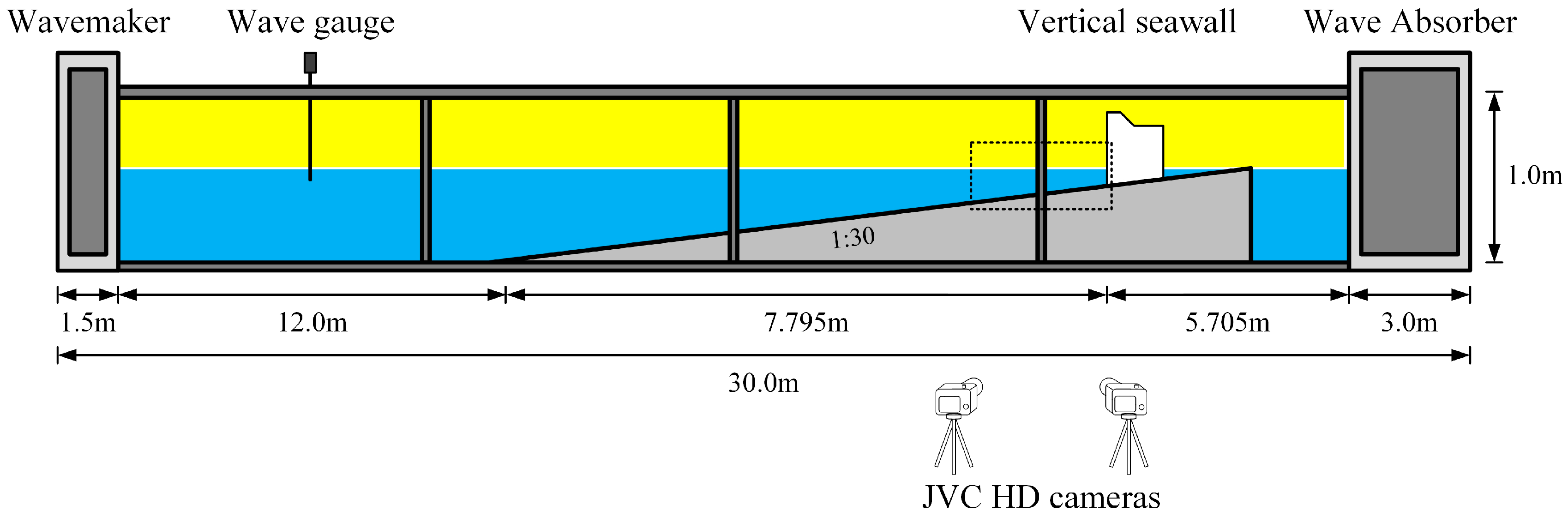
Laboratory experiments were performed in the two-dimensional wave flume at the University of Tokyo. The flume is 30 m long, 0.6 m wide, 1 m high and equipped with a piston-type wave maker as shown in Figure 2. A solid vertical wall as a vertical seawall was installed on a 1:30 sloping bed, whose surface material was smooth steel. The toe of the sloping bed and the vertical seawall was located at 12 m and 19.795 m from the wave maker. An original image-based measuring system was applied to capture the water surface fluctuations in the side glass wall plane as high-resolution data sets both in time and space domains. Two video cameras with high resolution capture of 1920 × 1080 pixels and a frame rate of 30 fps were used to record successive still images of the instantaneous water surface boundary along the cross section of about 2 m (two steel frames of the wave flume) near the seawall where the water and background were colored in blue and yellow, respectively. Obtained images were firstly rectified based on the eight reference points with actual XY-square-coordinates on the glass wall. Based on the RGB-values, which are the integer numbers stored in computers for indicating how much red, green, and blue is included in any human perceptional color, in each pixel, the surface water boundary was detected through the following parameter A:
For the present laboratory experiments, the yellow background should have large values of both R and G and small B since yellow is created by adding red to green and the blue water must have large B and small R and G. Therefore, the parameter A computed by Equation (12) should have larger values on the yellow background and smaller values on the blue water and decrease abruptly at the air-water boundary. In the laboratory experiments, A was always greater than 200 on the yellow background while less than 100 on the blue water even on the breaking and broken wave water where the water color tended to be brighter than the deeper water. Therefore, a single critical value A = 150 was used to determine the surface water boundary. Detected pixel coordinates of the water surface boundary were then transferred to the actual XY-coordinates on the glass wall of the flume. Validated by the data of wave gauges located at certain positions, it was shown that this image-based measuring system was able to capture surface fluctuations within acceptable errors both in non-breaking and breaking areas [32].
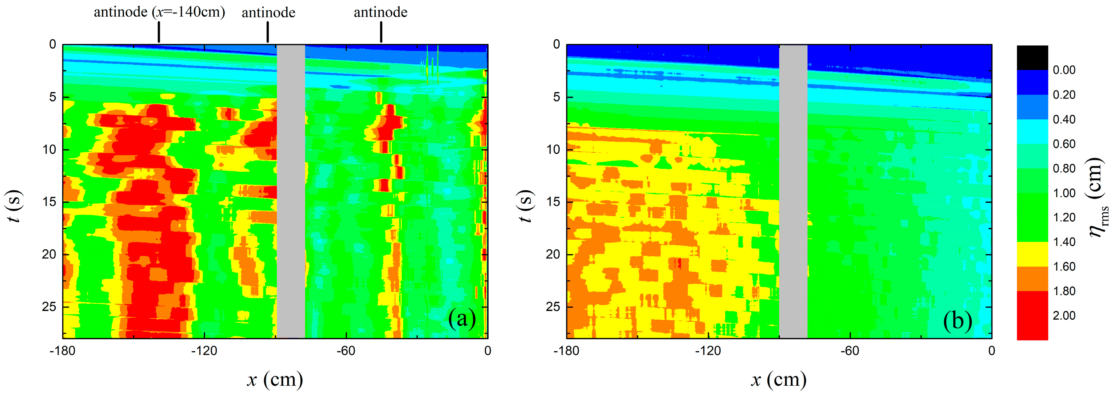
Five tests were run for regular waves with incident wave heights Hi varying from 4.2 cm to 5.5 cm, wave periods Ti from 1.2 s to 1.6 s and water depths at the seawall hs from 3 cm to 4.5 cm (water depth over flat bottom h from 30 cm to 31.5 cm). Incident wave conditions and water levels were designed to form broken waves with the presence of the seawall in which case waves start to break about 3/2 or one wave length from the seawall. For one wave case with Hi = 4.7 cm, Ti = 1.2 s, hs = 3 cm, progressive waves with the same incident wave conditions were also performed without the presence of the seawall for comparison. Figure 3 shows the time and spatial variation of root mean square of the surface water fluctuations, ηrms, near the seawall for the above-mentioned case and progressive wave case. ηrms was computed based on the extracted surface water level data of each single wave period so that time-variation of its values can be observed. The origin of the horizontal axis was set at the location of the seawall and the vertical axis is time. The gray color in Figure 3 represents the steel frame of wave flume, behind which no data was captured by the camera. As indicated by the red color in Figure 3a, antinodes of standing wave features can be successfully captured by the image-based measuring system. The positions of antinodes remain nearly the same, which implies steady partial standing waves form in front of the vertical seawall. It was also observed during the experiments that waves started to break around the antinode which is 3/2 wave length (i.e., around x = −140 cm) from the vertical wall. Compared to the progressive waves which start to break around x = −100 cm as indicated in Figure 3b, it can be seen that the formation of antinodes made the breaking points further from the vertical wall than the progressive wave case. More details about the image-based measuring system and data reports can be referred to Liu and Tajima [32].
4. Model-Data Comparison
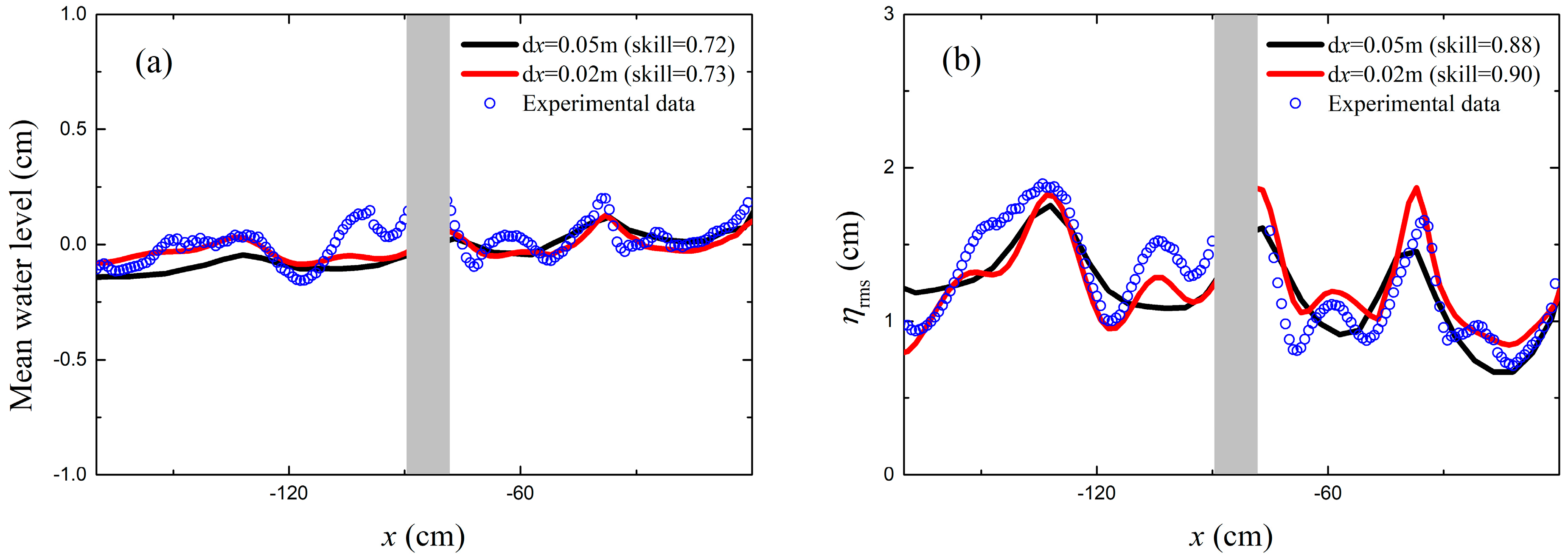
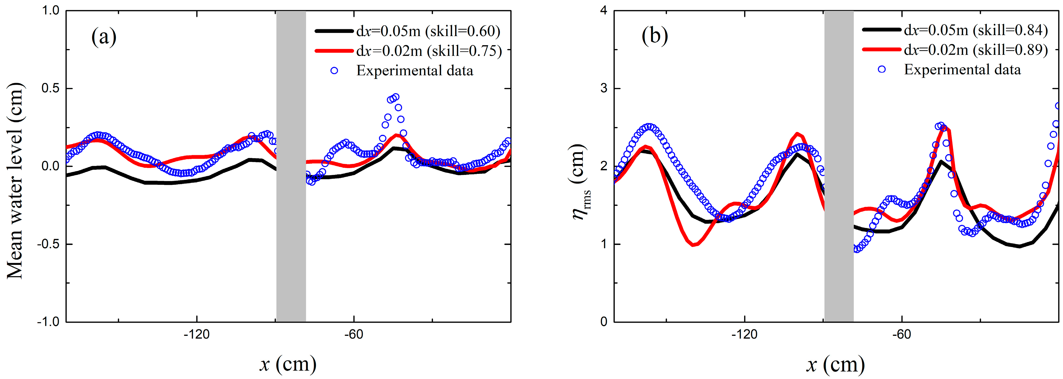
In model validation, model setup was the same as Liu and Tajima’s experiments. Shi et al. [35] have validated the present model with the laboratory experiments conducted by Hansen and Svendsen [42] for progressive wave shoaling and breaking with different breaking types over a uniform slope. It was found that the grid spacing is important for FUNWAVE-TVD, which uses the TVD technique in conjunction with a nonlinear shallow water equation to deal with wave breaking implicitly. The grid resolution is especially important to introduce the right amount of the energy dissipation at the breaking point. In Hansen and Svendsen’s experiments, regular waves with incident wave heights from 3.6 cm to 6.7 cm and wave periods from 1.0 s to 3.33 s were generated on a flat bottom with 0.36 m water depth and propagated over a 1:34.26 slope. Shi et al. [35] demonstrated the model could underestimate the peak wave height with a coarse grid size (i.e., dx = 0.05 m) compared to a fine grid size (i.e., dx = 0.02 m) due to numerical dissipation resulting from the coarse grid resolution. Since the experimental conditions, especially the wave lengths of incident waves of Liu and Tajima’s experiments, are similar to Hansen and Svendsen’s experiments, numerical results of these two grid sizes (dx = 0.05 m and dx = 0.02 m) are also presented in this study to demonstrate the sensitivity of the grid spacing. The value of Manning coefficient n employed in the bottom friction term was set to 0.012 for the smooth steel surface. Internal wavemaker [43] was implemented for incident regular waves and sponge layer was placed at the offshore side to absorb the reflected waves from the vertical seawall.
Validation results of two wave cases with Hi = 4.7 cm, Ti = 1.2 s, hs = 3 cm and Hi = 5.5 cm, Ti = 1.2 s, hs = 4.5 cm are presented here. Figure 4 and Figure 5 demonstrate the predicted and measured spatial distribution of mean water level and ηrms near the seawall for these two wave cases. Mean water level and ηrms were computed from the measured and predicted time series of surface fluctuations of ten wave cycles when waves reached a periodic equilibrium state. The origin of the horizontal axis was also set at the location of seawall. To quantify the performance of the model, the model skill is calculated as [44]:
where donates the predicted value, indicates the measured value, represents the mean measured value and N is the number of data points.
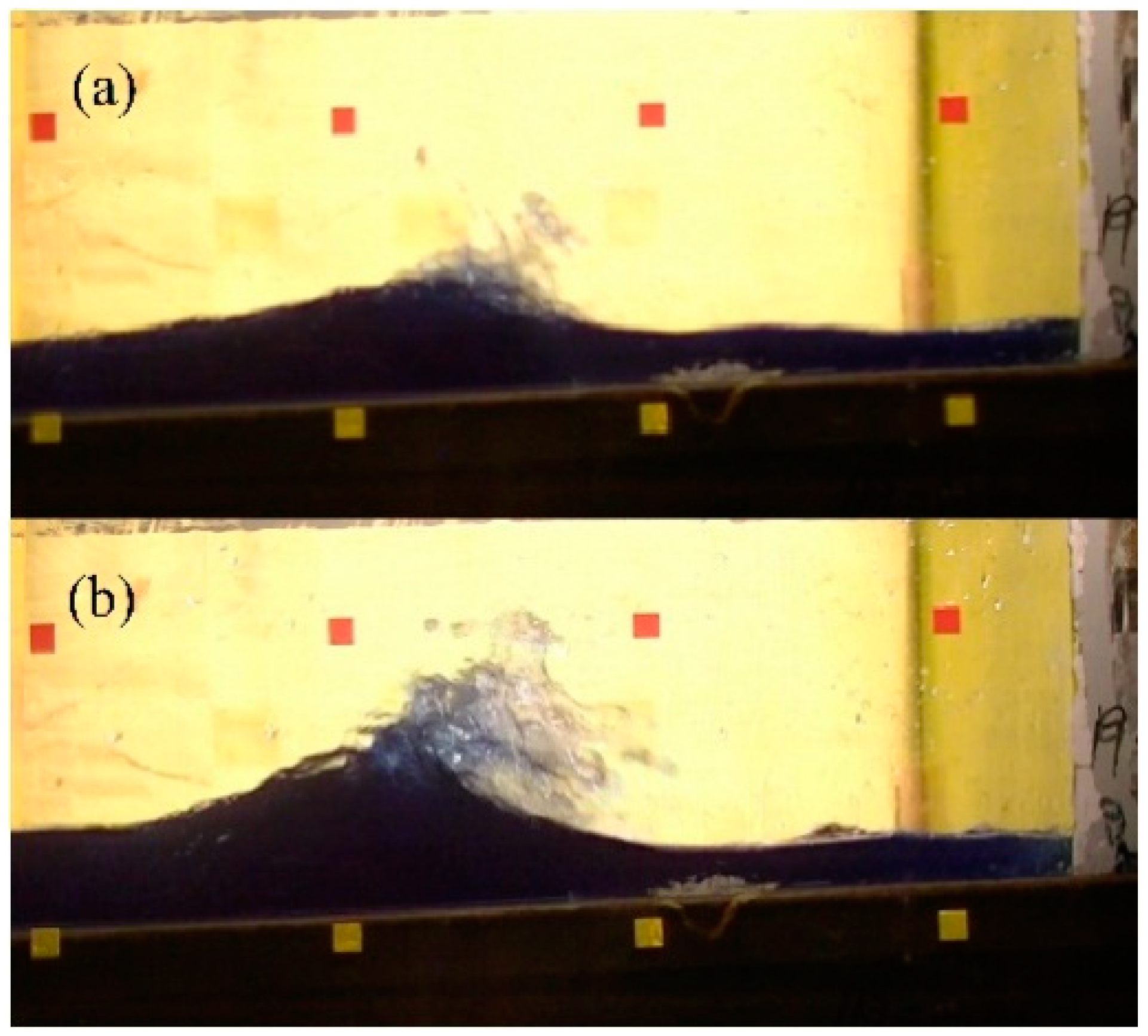
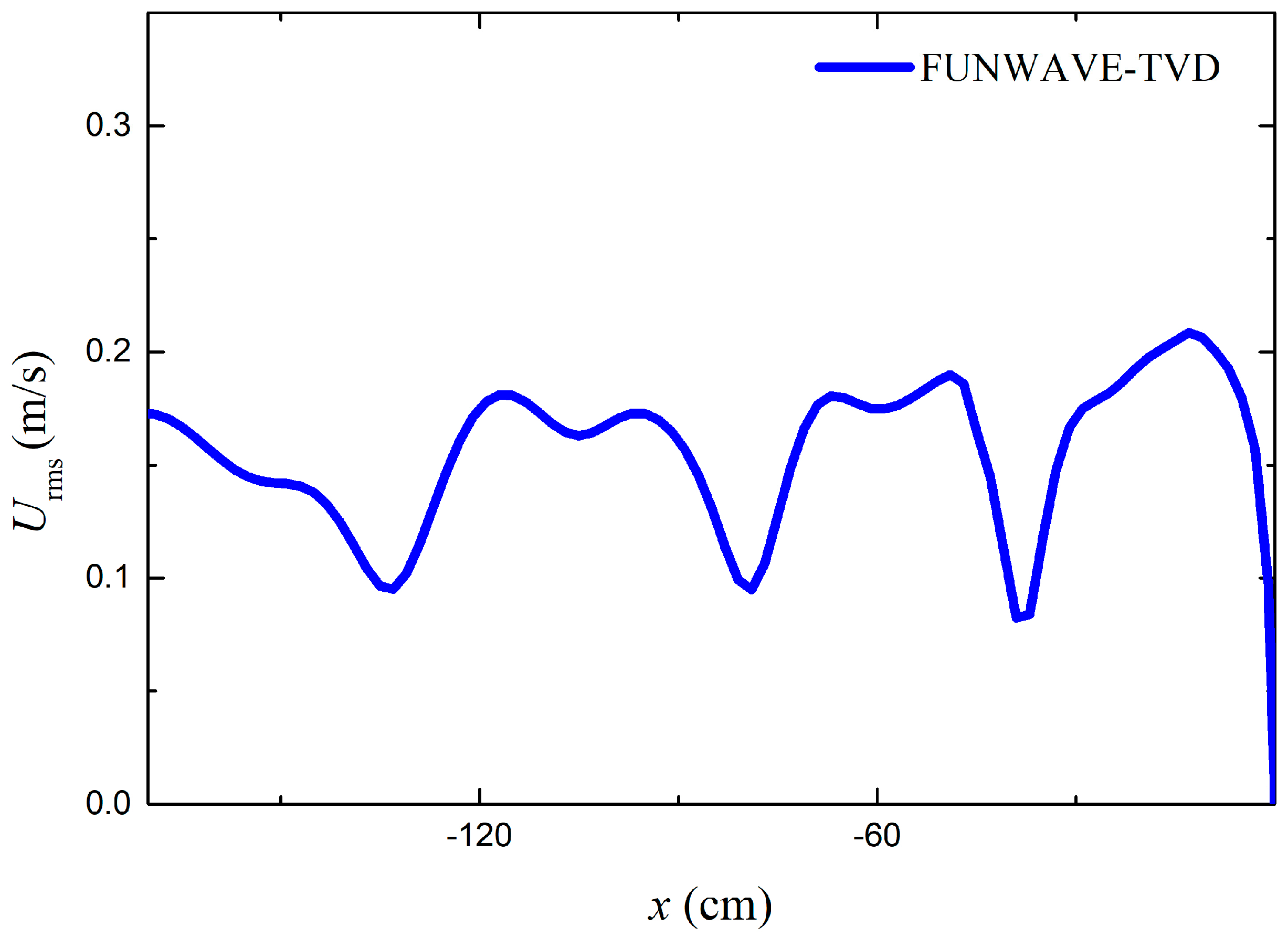
As shown in Figure 4 and Figure 5, the model with fine grid size (i.e., dx = 0.02 m) captures the characteristics of broken waves with reasonable accuracy. The formations of antinodes and their positions are well reproduced by the present model both in mean water level and ηrms. The coarse grid size tends to underpredict the peak of antinodes since wave breaking mainly happens around the antinodes under broken waves near a vertical seawall and coarse grid size leads to more numerical dissipation similar to the underprediction of peak wave height of progressive wave. In addition, it is noted in Figure 4 that the antinode of mean water level which is located at around x = −50 cm is obviously underestimated by the present model for the case with Hi = 5.5 cm, Ti = 1.2 s, hs = 4.5 cm. Figure 6 shows the typical snapshots of the collision of incident broken wave and reflected wave at this location (around x = −50 cm) for the wave case with Hi = 4.7 cm, Ti = 1.2 s, hs = 3 cm and wave case with Hi = 5.5 cm, Ti = 1.2 s, hs = 4.5 cm. As shown in Figure 6, the collision of broken incident waves and reflected waves in the case with Hi = 5.5 cm, Ti = 1.2 s, hs = 4.5 cm, which has larger incident wave height and increasing nonlinearity, becomes more violent at this location so that more water splashes out. The splashing water could be captured by the camera during the experiments, while it could not be simulated by the present model, resulting in an underestimation of mean water level by the model. Moreover, the splashing water released from the breaking antinodes also make the surface water fluctuations more complicated so that the present model still cannot reproduce the surface water profiles very accurately. Figure 7 shows the predicted spatial distribution of root mean square of depth-averaged horizontal velocity, Urms (U = P/D, the vector M in Equation (1) is defined as (P, Q) in the numerical scheme of the present model, in which case P and Q is the component of M along x direction and y direction), near the seawall. As seen in this figure, Urms is relatively smaller at the positions of antinodes, which confirms that the present model surely captures the key characteristics of partial standing wave near the seawall.
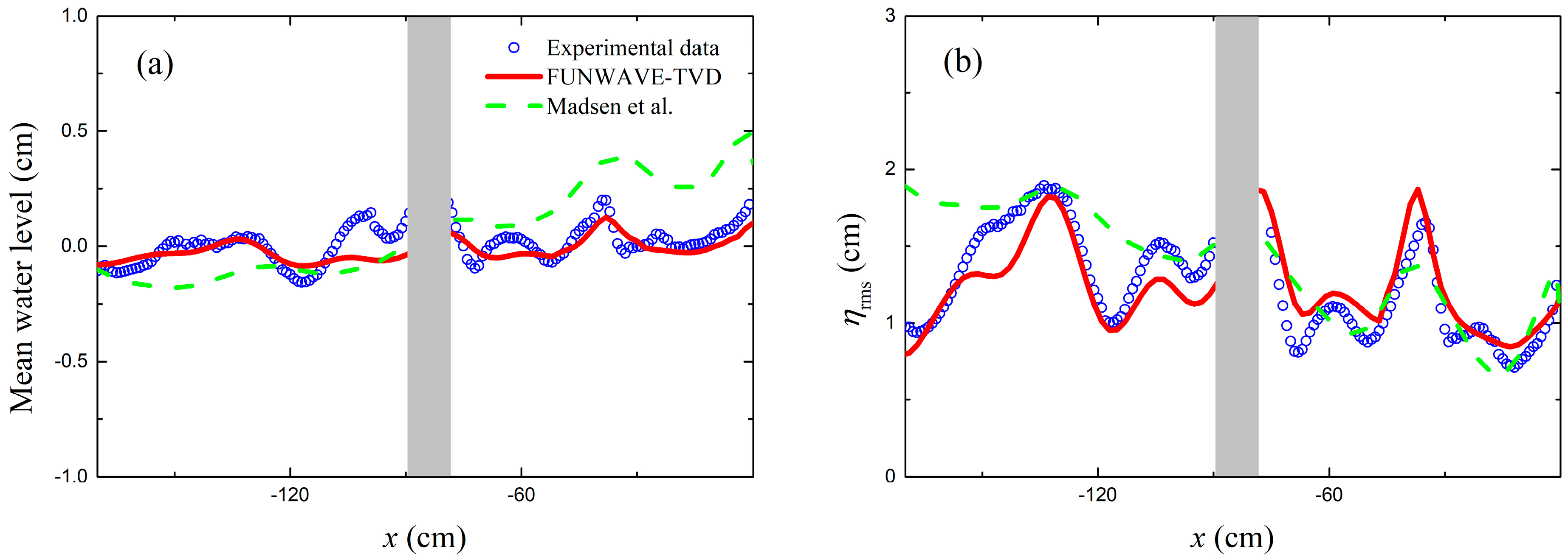
In order to further demonstrate the advantages of the shock-capturing method in predicting wave characteristics under broken waves near a seawall, comparisons of the numerical results obtained from the Boussinesq wave model with an empirical surface-roller breaking model [25] and the present model with dx = 0.02 m are presented in Figure 8 for the case with Hi = 4.7 cm, Ti = 1.2 s, hs = 3 cm. The notable model of Madsen et al. [25] has been successfully applied to model cross-shore motions of regular waves including various types of breaking on plane beaches and over submerged bars. It is also reported the surface roller type breaking model demonstrates the most appropriate predictive skills of time-varying profiles of surface water compared to the other empirical breaking models [28]. As seen in Figure 8, for the present study, mean water level predicted by the surface-roller breaking model has an obvious setup after wave breaking while ηrms has an obvious decreasing trend. It is also noted that the profile of ηrms predicted by the surface-roller model becomes smoother than the ones of FUNWAVE-TVD and experimental data, especially at the left part of the figure (i.e., −180 < x < −100 cm). As revealed in Liu and Tajima [32], empirical breaking models including surface-roller model and eddy-viscosity model developed based on the progressive wave assumptions take the whole partial standing wave field as pure progressive waves with their breaking criteria and simulated energy dissipation happens both in incident waves and reflected waves while experimental data indicates that dissipation of reflected waves is insignificant actually. Therefore, excess dissipation computed by these breaking models leads to an obvious setup and decreasing of ηrms and smaller reflected waves lead to a smoother profile of ηrms. To the authors’ delight, the present model using shock-capturing method improves these features. The results presented here indicate the shock-capturing method using the ratio of wave height to the local depth as the breaking criteria is more appropriate for modeling the broken waves near a vertical seawall by eliminating the excess dissipation in reflected waves.
5. Numerical Experiment Results
As seen in Table 1, the wave types in front of vertical seawalls are mainly determined by the wave height, water depth at the seawall, and the seabed slope. Thus, after validation of the model, a series of numerical experiments were implemented to investigate the effects of these key parameters, such as the incident wave height Hi, wave depth at the vertical seawall hs, and bed slope tanθ, on the wave kinematics (i.e., the root mean square of the surface fluctuations and depth-averaged horizontal velocity) under broken waves near vertical seawalls. Numerical experiment setup is shown in Figure 9. The internal wave maker is 20 m from the seawall and the computational domain with a total length of 26 m is applied with a 3 m sponge layer at the offshore side. The numerical experimental wave conditions for all model runs are listed in Table 3. The tested range of parameters in this numerical study is designed based on the Froude similarity with a geometric scale factor of 1:100. Therefore, at the prototype scale, incident wave heights are from 4 m to 10 m, representing the typical wave heights during typhoon and super typhoon and wave depths at the vertical seawall are from 2 m to 6 m, representing the typical water depths near the vertical seawall subjected to broken waves. For each group in Table 3, only one parameter was changed while keeping other parameters the same. Grid size dx = 0.02 m, Manning coefficient n = 0.012 were used in all numerical experiments as validated above.
Figure 10 shows the computed spatial distributions of ηrms and Urms near the seawall for Cases 1–3 of Group 1 whose incident wave heights are 0.04 m, 0.07 m and 0.1 m respectively. Urms can be somehow regarded as a physically relevant indicator of the potential surrounding scour and wave impact on the seawall. As seen in Figure 10a, the positions of antinodes are nearly the same for these wave cases since they have the same dispersion relationship. It is noted both Case 1 and Case 2 start to break at the antinode around x = −0.5 m, which is 1/2 wave length from the seawall since the elevations of antinodes forming near the seawall continues to increase. For these two wave cases, larger incident wave height induces higher ηrms near the seawall and higher runup on the seawall consequently. On the other hand, waves of Case 3 with the largest incident wave height, 0.1 m, in this group break further from the seawall at the antinode around x = −1.75 m, which is 3/2 wave length from the seawall. However, ηrms of Case 2 and Case 3 become nearly the same between the antinode at around x = −0.5 m and the seawall and the consequent runups on the seawall of these two cases are also close. As seen in Figure 10b, similar to ηrms, for Case 1 and Case 2, which break at the same location, incident wave with larger incident wave height induces higher Urms near the seawall and for Case 2 and Case 3 Urms are nearly the same near the seawall.
Figure 11 shows the computed spatial distributions of ηrms and Urms near the seawall for Cases 4–6 in Group 2 whose water levels at the seawall, hs, are 6 cm, 4 cm and 2 cm respectively. hs is adjusted by changing the deep-water depth over flat bottom in this study. As seen in Figure 11a, the positions of antinodes are different for these wave cases due to different dispersion relationships. Locations of breaking points move further quickly from the seawall as hs decreases, in which case the ηrms near the seawall and runups on the seawall also decrease significantly. As seen in Figure 11b, shallower hs induces smaller Urms near the seawall as well.
Figure 12 shows the computed spatial distributions of ηrms and Urms near the seawall for Cases 7–10 in Group 3 whose bed slope angles, tanθ, are 1:15, 1:20, 1:25 and 1:30 respectively. As seen in Figure 12a, the positions of antinodes are slightly different for these wave cases and the locations of breaking points are all at the antinodes which are 1/2 wave length from the seawall. Spatial distributions of the ηrms do not vary much as the seabed slope changes and the runups on the seawall get a little smaller when the bed slope becomes milder. As seen in Figure 12b, Urms also seem insensitive to the seabed slope.
6. Discussions and Conclusions
In this paper, the fully nonlinear Boussinesq wave model FUNWAVE-TVD was applied to model wave characteristics under broken waves in front of a vertical seawall. Validation with the experimental data confirmed the ability of FUNWAVE-TVD in capturing the key characteristics in such conditions using a shock-capturing method. The grid size is important to predict the peak height around the antinodes accurately. The shock-capturing method is more appropriate for modeling the broken waves near a seawall than the empirical breaking model based on progressive wave assumptions. As the Boussinesq-type models only yield the velocity based on potential flow theory, additional flow model can be further coupled for predictions of the vertical profile of the horizontal shear velocity field, which is necessary for estimations of surrounding scour and cross-shore sediment transport. In this study, a preliminary investigation of the effects of the key parameters, such as the incident wave height, water level at the seawall, and seabed slope, on the wave kinematics (i.e., the root mean square of the surface fluctuations and depth-averaged horizontal velocity) near vertical seawalls was conducted through a series of numerical experiments.
The numerical experiment results from this study suggest the incident wave height and the water depth at the seawall are the important parameters in determining the magnitude of the wave kinematics near the seawall. The role of the breaking point locations is also highlighted in this study. When incident waves have the same breaking locations, larger incident wave height can induce larger wave kinematics near the seawall, in which case the potential surrounding scour and wave impact on the seawall are larger. However, the breaking point can move further from the seawall as the incident wave height increases and the wave kinematics near the seawall can be mitigated by this further breaking.
Over a uniform plane beach, locations of breaking points seem to be more sensitive to the water depth at the seawall. The breaking point moves further from the seawall quickly as the water depth at the seawall gets shallow, and as a result, the magnitude of the wave kinematics near the seawall decrease significantly. This implies seawalls subjected to the broken waves are under higher risk during the high water-level events, such as the high tide and storm surge. The rising sea-level due to the climate change which results in a net increase in water depth at the seawall will endanger the coastal structures as well. Moreover, the water depth at the seawall can be adjusted as the locations of seawalls change. Therefore, seawalls which are planned to build at the back of the beach and predominantly subjected to broken waves should be well considered for their construction sites if possible.
The seabed slope seems to be insignificant, affecting the wave kinematics near the seawall. The authors must state that natural beaches are more complex than the idealized uniform beaches used in this study. A realistic nearshore bathymetry which may significantly affect the breaking points should modify the results in this study. Furthermore, artificial obstacles, such as submerged breakwaters, which are placed in front of seawalls to make the wave breaking earlier, may be an efficient way to reduce the structural risk induced by broken waves.
Author Contributions
Numerical simulations and data analysis were completed by W.L., Y.N., Y.Z. and J.Z. Draft was prepared by W.L.
Funding
This work was funded by the National Natural Science Foundation of China (grant numbers 51609043, 51809234), the Key Laboratory of Water-Sediment Sciences and Water Disaster Prevention of Hunan Province (under the awards 2018SS03), the Key Laboratory of Coastal Disaster and Defense, Ministry of Education, China (under the awards 201708) and the Bureau of Science and Technology of Zhoushan (under the awards 2018C81040).
Conflicts of Interest
The authors declare no conflict of interest.
References
- Gao, X.; Inouchi, K. The characteristics of scouring and depositing in front of vertical breakwaters by broken clapotis. Coast. Eng. J. 1998, 40, 99–113. [Google Scholar] [CrossRef]
- Oumeraci, H.; Klammer, P.; Partenscky, H.W. Classification of breaking wave loads on vertical structures. J. Waterw. Port Coast. Ocean Eng. 1993, 119, 381–397. [Google Scholar] [CrossRef]
- Goda, Y. Dynamic response of upright breakwaters to impulsive breaking wave forces. Coast. Eng. 1994, 22, 135–158. [Google Scholar] [CrossRef]
- Oumeraci, H.; Kortenhaus, A. Analysis of the dynamic response of caisson breakwaters. Coast. Eng. 1994, 22, 159–183. [Google Scholar] [CrossRef]
- Oumeraci, H.; Kortenhaus, A. Wave impact loading: Tentative formulae and suggestions for the development of final formulae. In Proceedings of the 2nd Task 1 MAST III Workshop (PROVERBS), Edingburgh, UK, 2–4 July 1997. [Google Scholar]
- Karim, M.F.; Tingsanchali, T. A coupled numerical model for simulation of wave breaking and hydraulic performances of a composite seawall. Ocean Eng. 2006, 33, 773–787. [Google Scholar] [CrossRef]
- Bullock, G.N.; Obhrai, C.; Peregrine, D.H.; Bredmose, H. Violent breaking wave impacts. Part 1: Results from large-scale regular wave tests on vertical and sloping walls. Coast. Eng. 2007, 54, 602–617. [Google Scholar] [CrossRef]
- Cuomo, G.; Allsop, W.; Bruce, T.; Pearson, J. Breaking wave loads at vertical seawalls and breakwaters. Coast. Eng. 2010, 57, 424–439. [Google Scholar] [CrossRef]
- Mokrani, C.; Abadie, S.; Grilli, S.T.; Zibouche, K. Numerical Simulation of the Impact of a Plunging Breaker On a Vertical Structure and Subsequent Overtopping Event Using a Navier-Stokes VOF Model. In Proceedings of the Twentieth International Offshore and Polar Engineering Conference, Beijing, China, 20–25 June 2010; p. 8. [Google Scholar]
- Kisacik, D.; Troch, P.; Van Bogaert, P. Experimental study of violent wave impact on a vertical structure with an overhanging horizontal cantilever slab. Ocean Eng. 2012, 49, 1–15. [Google Scholar] [CrossRef]
- Ramachandran, K. Broken wave loads on a vertical wall: Large scale experimental investigations. In Proceedings of the 6th International Conference on Structural Engineering and Construction Management, Kandy, Sri Lanka, 11–13 December 2015. [Google Scholar]
- Van Dongeren, A.R.; Sancho, F.E.; Svendsen, I.A.; Putrevu, U. SHORECIRC: A Quasi 3-D Nearshore Model. Coast. Eng. Proc. 1994. [Google Scholar] [CrossRef]
- Tajima, Y.; Madsen, O.S. Modeling Near-Shore Waves, Surface Rollers, and Undertow Velocity Profiles. J. Waterw. Port Coast. Ocean Eng. 2006, 132, 429–438. [Google Scholar] [CrossRef]
- Bradford, S.F. Numerical Simulation of Surf Zone Dynamics. J. Waterw. Port Coast. Ocean Eng. 2000, 126, 1–13. [Google Scholar] [CrossRef]
- Christensen, E.D.; Walstra, D.-J.; Emerat, N. Vertical variation of the flow across the surf zone. Coast. Eng. 2002, 45, 169–198. [Google Scholar] [CrossRef]
- Zhao, X.; Ye, Z.; Fu, Y.; Cao, F. A CIP-based numerical simulation of freak wave impact on a floating body. Ocean Eng. 2014, 87, 50–63. [Google Scholar] [CrossRef]
- Madsen, P.A.; Sørensen, O.R. A new form of the Boussinesq equations with improved linear dispersion characteristics. Part 2. A slowly-varying bathymetry. Coast. Eng. 1992, 18, 183–204. [Google Scholar] [CrossRef]
- Nwogu, O. Alternative form of Boussinesq equations for nearshore wave propagation. J. Waterw. Port Coast. Ocean Eng. 1993, 119, 618–638. [Google Scholar] [CrossRef]
- Wei, G.; Kirby, J.T.; Grilli, S.T.; Subramanya, R. A fully nonlinear Boussinesq model for surface waves. Part 1. Highly nonlinear unsteady waves. J. Fluid Mech. 1995, 294, 71–92. [Google Scholar] [CrossRef]
- Zhang, Y.; Kennedy, A.B.; Panda, N.; Dawson, C.; Westerink, J.J. Boussinesq–Green–Naghdi rotational water wave theory. Coast. Eng. 2013, 73, 13–27. [Google Scholar] [CrossRef]
- Peregrine, D.H. Long waves on a beach. J. Fluid Mech. 1967, 27, 815–827. [Google Scholar] [CrossRef]
- Nwogu, O. Numerical prediction of breaking waves and currents with a Boussinesq model. In Proceedings of the 25th Conference on Coastal Engineering, Orlando, FL, USA, 2–6 September 1996. [Google Scholar]
- Kennedy, A.B.; Chen, Q.; Kirby, J.T.; Dalrymple, R.A. Boussinesq modeling of wave transformation, breaking, and runup. I: 1D. J. Waterw. Port Coast. Ocean Eng. 2000, 126, 39–47. [Google Scholar] [CrossRef]
- Schäffer, H.A.; Madsen, P.A.; Deigaard, R. A Boussinesq model for waves breaking in shallow water. Coast. Eng. 1993, 20, 185–202. [Google Scholar] [CrossRef]
- Madsen, P.A.; Sørensen, O.R.; Schäffer, H.A. Surf zone dynamics simulated by a Boussinesq type model. Part I. Model description and cross-shore motion of regular waves. Coast. Eng. 1997, 32, 255–287. [Google Scholar] [CrossRef]
- Bredmose, H.; Schäffer, H.A.; Madsen, P.A. Boussinesq evolution equations: Numerical efficiency, breaking and amplitude dispersion. Coast. Eng. 2004, 51, 1117–1142. [Google Scholar] [CrossRef]
- Chen, Q.; Kirby, J.T.; Dalrymple, R.A.; Shi, F.; Thornton, E.B. Boussinesq modeling of longshore currents. J. Geophys. Res. Oceans 2003, 108. [Google Scholar] [CrossRef] [Green Version]
- Mohsin, S.; Tajima, Y. Modeling of time-varying shear current field under breaking and broken waves with surface rollers. Coast. Eng. J. 2014, 56, 1450013. [Google Scholar] [CrossRef]
- Yao, Y.; Becker, J.M.; Ford, M.R.; Merrifield, M.A. Modeling wave processes over fringing reefs with an excavation pit. Coast. Eng. 2016, 109, 9–19. [Google Scholar] [CrossRef] [Green Version]
- Zhang, Y.; Kennedy, A.B.; Tomiczek, T.; Donahue, A.; Westerink, J.J. Validation of Boussinesq–Green–Naghdi modeling for surf zone hydrodynamics. Ocean Eng. 2016, 111, 299–309. [Google Scholar] [CrossRef] [Green Version]
- Zhang, S.; Zhu, L.; Li, J. Numerical Simulation of Wave Propagation, Breaking, and Setup on Steep Fringing Reefs. Water 2018, 10, 1147. [Google Scholar] [CrossRef]
- Liu, W.; Tajima, Y. Image-based study of breaking and broken characteristics in front of a vertical seawall. In Proceedings of the 34th Conference on Coastal Engineering, Seoul, Korea, 15–20 June 2014. [Google Scholar]
- Tonelli, M.; Petti, M. Simulation of wave breaking over complex bathymetries by a Boussinesq model. J. Hydraul. Res. 2011, 49, 473–486. [Google Scholar] [CrossRef]
- Roeber, V.; Cheung, K. Boussinesq-type model for energetic breaking waves in fringing reef environments. Coast. Eng. 2012, 70, 1–20. [Google Scholar] [CrossRef]
- Shi, F.; Kirby, J.T.; Harris, J.C.; Geiman, J.D.; Grilli, S.T. A high-order adaptive time-stepping TVD solver for Boussinesq modeling of breaking waves and coastal inundation. Ocean Model. 2012, 43–44, 36–51. [Google Scholar] [CrossRef]
- Fang, K.; Liu, Z.; Zou, Z. Fully nonlinear modeling wave transformation over fringing reefs using shock-capturing Boussinesq model. J. Coast. Res. 2016, 32, 164–171. [Google Scholar] [CrossRef]
- Su, S.-F.; Ma, G.; Hsu, T.-W. Boussinesq modeling of spatial variability of infragravity waves on fringing reefs. Ocean Eng. 2015, 101, 78–92. [Google Scholar] [CrossRef]
- Chen, Q. Fully nonlinear Boussinesq-type equations for waves and currents over porous beds. J. Eng. Mech. 2006, 132, 220–230. [Google Scholar] [CrossRef]
- Kennedy, A.B.; Kirby, J.T.; Chen, Q.; Dalrymple, R.A. Boussinesq-type equations with improved nonlinear performance. Wave Motion 2001, 33, 225–243. [Google Scholar] [CrossRef] [Green Version]
- Tonelli, M.; Petti, M. Hybrid finite volume—Finite difference scheme for 2DH improved Boussinesq equations. Coast. Eng. 2009, 56, 609–620. [Google Scholar] [CrossRef]
- Yao, Y.; Huang, Z.; Monismith, S.G.; Lo, E.Y.M. 1DH Boussinesq modeling of wave transformation over fringing reefs. Ocean Eng. 2012, 47, 30–42. [Google Scholar] [CrossRef]
- Hansen, J.B.; Svendsen, I.A. Regular Waves in Shoaling Water: Experimental Data; Technical University of Denmark: Lyngby, Denmark, 1979. [Google Scholar]
- Wei, G.; Kirby, J.T.; Sinha, A. Generation of waves in Boussinesq models using a source function method. Coast. Eng. 1999, 36, 271–299. [Google Scholar] [CrossRef] [Green Version]
- Willmott, C.J. On the validation of models. Phys. Geogr. 1981, 2, 184–194. [Google Scholar] [CrossRef]
Figure 1.
Three wave types in front of vertical seawalls [1]. (a) non-breaking standing waves; (b) breaking waves; (c) broken waves.
Figure 1.
Three wave types in front of vertical seawalls [1]. (a) non-breaking standing waves; (b) breaking waves; (c) broken waves.

Figure 2.
Experimental setup.

Figure 3.
Time and spatial variation of the root mean square of the surface fluctuations near the seawall for (a) broken waves and (b) progressive waves.
Figure 3.
Time and spatial variation of the root mean square of the surface fluctuations near the seawall for (a) broken waves and (b) progressive waves.

Figure 4.
Comparisons of predicted and measured spatial distribution of (a) mean water level and (b) ηrms for the wave case with Hi = 4.7 cm, Ti = 1.2 s, hs = 3 cm.
Figure 4.
Comparisons of predicted and measured spatial distribution of (a) mean water level and (b) ηrms for the wave case with Hi = 4.7 cm, Ti = 1.2 s, hs = 3 cm.

Figure 5.
Comparisons of predicted and measured spatial distribution of (a) mean water level and (b) ηrms for the wave case with Hi = 5.5 cm, Ti = 1.2 s, hs = 4.5 cm.
Figure 5.
Comparisons of predicted and measured spatial distribution of (a) mean water level and (b) ηrms for the wave case with Hi = 5.5 cm, Ti = 1.2 s, hs = 4.5 cm.

Figure 6.
Typical snapshots of the collision of incident broken wave and reflected wave for (a) the wave case with Hi = 4.7 cm, Ti = 1.2 s, hs = 3 cm and (b) wave case with Hi = 5.5 cm, Ti = 1.2 s, hs = 4.5 cm.
Figure 6.
Typical snapshots of the collision of incident broken wave and reflected wave for (a) the wave case with Hi = 4.7 cm, Ti = 1.2 s, hs = 3 cm and (b) wave case with Hi = 5.5 cm, Ti = 1.2 s, hs = 4.5 cm.

Figure 7.
Predicted spatial distribution of root mean square of depth-averaged horizontal velocity near the seawall.
Figure 7.
Predicted spatial distribution of root mean square of depth-averaged horizontal velocity near the seawall.

Figure 8.
Comparisons of predicted spatial distribution of (a) mean water level and (b) ηrms between Madsen et al. [25] and FUNWAVE-TVD for the wave case with Hi = 4.8 cm, Ti = 1.2 s, hs = 3 cm.
Figure 8.
Comparisons of predicted spatial distribution of (a) mean water level and (b) ηrms between Madsen et al. [25] and FUNWAVE-TVD for the wave case with Hi = 4.8 cm, Ti = 1.2 s, hs = 3 cm.

Figure 9.
Numerical experiment setup.

Figure 10.
Computed spatial distributions of (a) ηrms and (b) Urms near the seawall for Cases 1–3.

Figure 11.
Computed spatial distributions of (a) ηrms and (b) Urms near the seawall for Cases 4–6.

Figure 12.
Computed spatial distributions of (a) ηrms and (b) Urms near the seawall for Cases 7–10.


Table 1.
The conditions to form three wave types in front of a vertical seawall.
| The Size of Foundation-Bed | Forming Conditions | Wave Type |
|---|---|---|
| h1/hs ≥ 2/3 | hs ≥ 2H | Non-breaking standing waves |
| hs < 2H, i ≤ 1/10 | Broken waves | |
| 2/3 ≥ h1/hs > 1/3 | h1 ≥ 1.8H | Non-breaking standing waves |
| h1 < 1.8H | Breaking waves | |
| h1/hs ≤ 1/3 | h1 ≥ 1.5H | Non-breaking standing waves |
| h1 < 1.5H | Breaking waves |
Note: H is the progressive wave height at a vertical seawall, hs is the water depth at a vertical seawall, h1 is the water depth above the foundation-bed, i is the seabed slope.
Table 2.
Three categories of existing models for predictions of nearshore wave hydrodynamics.
| Category No. | Governing Equations | Scope of Application | Deficiency |
|---|---|---|---|
| 1 | Energy-balanced equations | Phase-averaged nearshore current field | Limited to the phenomena suitable for linear wave assumptions |
| 2 | Navier–Stokes equations | Velocity filed and wave impact associated with wave-structure interactions | Limited to the small-scale phenomena due to the high cost of computation |
| 3 | Boussinesq equations with an ad-hoc dissipation term | Near shore wave processes, including shoaling, dissipation, diffraction, refraction and reflection | Limited to the progressive waves due to the applicability of empirical breaking models |
Table 3.
Numerical experimental wave conditions.
| Hi (m) | hs (cm) | tanθ | Ti (s) | ||
|---|---|---|---|---|---|
| Group 1 | Case 1 | 0.04 | 6.0 | 1:30 | 1.2 |
| Case 2 | 0.07 | 6.0 | 1:30 | 1.2 | |
| Case 3 | 0.1 | 6.0 | 1:30 | 1.2 | |
| Group 2 | Case 4 | 0.07 | 6.0 | 1:30 | 1.2 |
| Case 5 | 0.07 | 4.0 | 1:30 | 1.2 | |
| Case 6 | 0.07 | 2.0 | 1:30 | 1.2 | |
| Group 3 | Case 7 | 0.07 | 6.0 | 1:15 | 1.2 |
| Case 8 | 0.07 | 6.0 | 1:20 | 1.2 | |
| Case 9 | 0.07 | 6.0 | 1:25 | 1.2 | |
| Case 10 | 0.07 | 6.0 | 1:30 | 1.2 |
© 2018 by the authors. Licensee MDPI, Basel, Switzerland. This article is an open access article distributed under the terms and conditions of the Creative Commons Attribution (CC BY) license (http://creativecommons.org/licenses/by/4.0/).
Share and Cite
MDPI and ACS Style
Liu, W.; Ning, Y.; Zhang, Y.; Zhang, J. Shock-Capturing Boussinesq Modelling of Broken Wave Characteristics Near a Vertical Seawall. Water 2018, 10, 1876. https://doi.org/10.3390/w10121876
AMA Style
Liu W, Ning Y, Zhang Y, Zhang J. Shock-Capturing Boussinesq Modelling of Broken Wave Characteristics Near a Vertical Seawall. Water. 2018; 10(12):1876. https://doi.org/10.3390/w10121876
Chicago/Turabian StyleLiu, Weijie, Yue Ning, Yao Zhang, and Jiandong Zhang. 2018. "Shock-Capturing Boussinesq Modelling of Broken Wave Characteristics Near a Vertical Seawall" Water 10, no. 12: 1876. https://doi.org/10.3390/w10121876
Note that from the first issue of 2016, this journal uses article numbers instead of page numbers. See further details here.